An objective function for self-limiting neural plasticity rules.

Abstract

Self-organization provides a framework for the study of systems in which complex patterns emerge from simple rules, without the guidance of external agents or fine tuning of parameters. Within this framework, one can formulate a guiding principle for plasticity in the context of unsupervised learning, in terms of an objective function. In this work we derive Hebbian, self-limiting synaptic plasticity rules from such an objective function and then apply the rules to the non-linear bars problem.

1 Introduction

Hebbian learning rules [1] are at the basis of unsupervised learning in neural networks, involving the adaption of the inter-neural synaptic weights [2, 3]. These rules usually make use of either an additional renormalization step or a decay term in order to avoid runaway synaptic growth [4, 5].

From the perspective of self-organization [6, 7, 8, 9], it is interesting to study how Hebbian, self-limiting synaptic plasticity rules can emerge from a set of governing principles, in terms of objective functions. Information theoretical measures such as the entropy of the output firing rate distribution have been used in the past to generate rules for either intrinsic or synaptic plasticity [10, 11, 12]. The objective function with which we work here can be motivated from the Fisher information, which measures the sensitivity of a certain probability distribution to a parameter, in this case defined with respect to the Synaptic Flux operator [13], which measures the overall increase of synaptic weights. Minimizing the Fisher information corresponds, in this context, to looking for a steady state solution where the output probability distribution is insensitive to local changes in the synaptic weights. This method, then constitutes an implementation of the stationarity principle, stating that once the features of a stationary input distribution have been acquired, learning should stop, avoiding runaway growth of the synaptic weights.

It is important to note that, while in other contexts the Fisher information is maximized to estimate a certain parameter via the Cramér-Rao bound, in this case the Fisher information is defined with respect to the model’s parameters, which do not need to be estimated, but rather adjusted to achieve a certain goal. This procedure has been successfully employed in the past in other fields to derive, for instance, the Schrödinger Equation in Quantum Mechanics [14].

2 Methods

We consider rate-encoding point neurons, where the output activity $y$ of each neuron is a sigmoidal function of its weighed inputs, as defined by:

$$y=g(x),\qquad x=\sum_{j=1}^{N_{w}}w_{j}(y_{j}-\bar{y}_{j}).$$ (1)

Here the $y_{j}s$ are the $N_{w}$ inputs to the neuron (which will be either the outputs of other neurons or external stimuli), the $w_{j}$ are the synaptic weights, and $x$ the integrated input, which one may consider as the neuron’s membrane potential. $\bar{y}_{j}$ represents the average of input $y_{j}$, so that only deviations from the average convey information. $g$ represents here a sigmoidal transfer function, such that $g(x)\longrightarrow 1/0$ when $x\longrightarrow\pm\infty$. The output firing rate $y$ of the neuron is hence a sigmoidal function of the membrane potential $x$.

By minimization through stochastic gradient descent of:

$$F_{ob}\ =\ E\big{[}f_{ob}(x)\big{]}\ =\ E\left[\big{(}N+A(x)\big{)}^{2}\right],\qquad A(x)=\frac{xy^{\prime\prime}}{y^{\prime}}~{},$$ (2)

a Hebbian self-limiting learning rule for the synaptic weights can be obtained [13]. Here $E[.]$ denotes the expected value, as averaged over the probability distribution of the inputs, and $y^{\prime}$ and $y^{\prime\prime}$ are respectively the first and second derivatives of $y(x)$. $N$ is a parameter of the model (originally derived as $N_{w}$ and then generalized [13]), which sets the values for the system’s fixed-points, as shown in Section 2.1.

In the case of an exponential, or Fermi transfer function, we obtain

$$g_{exp}(x)\ =\ \frac{1}{1+exp(b-x)},\qquad\quad f_{ob}\ =\ \Big{(}N+x\big{(}1-2y(x)\big{)}\Big{)}^{2}$$ (3)

for the kernel $f_{ob}$ of the objective function $F_{ob}$. The intrinsic parameter $b$ represents a bias and sets the average activity level of the neuron. This parameter can either be kept constant, or adapted with little interference by other standard procedures such as maximizing the output entropy [10, 13].

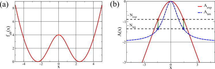
Figure 1: (a) $f_{ob}(x)$, as defined by Eq. (3), for $b=0$ and $N=2$. The synaptic weights are adapted through (4) such that the membrane potential $x$ tends to cluster around the two minima. (b) $A(x)$, as defined by Eqs. (2) and (7), for both the exponential and the tangential sigmoidal transfer functions and $b=0$. Adapting the respective values of $N$ identical roots can be obtained, as illustrated graphically.

In Fig. 1(a) the functional dependence of $f_{ob}$ is shown. It diverges for $x\longrightarrow\pm\infty$ and minimizing $f_{ob}$ will hence keep $x$, and therefore the synaptic weights, bound to finite values. Minimizing (3) through stochastic gradient descent with respect to $w_{j}$, one obtains [13]:

$$\dot{w}_{j}\ =\ \epsilon_{w}G(x)H(x)(y_{j}-\bar{y}_{j})$$ (4)

$$G(x)=N+x(1-2y),\qquad\quad H(x)=(2y-1)+2x(1-y)y$$ (5)

where the product $H(x)(y_{j}-\bar{y}_{j})$ represents the Hebbian part of the update rule, with $H$ being an increasing function of $x$ or $y$, and where $G$ reverses the sign when the activity is too large to avoid runaway synaptic growth.

2.1 Minima of the objective function

While (2) depends quantitatively on the specific choice of the transfer function $g$, we will show here how the resulting expression for different transfer functions are in the end similar. We compare here as an example two choices for $g$, the exponential sigmoidal (or Fermi function) defined in (3), and a arc-tangential transfer function defined as:

$$g_{tan}(x)\ =\ \frac{1}{\pi}arctan(x-b)+1/2.$$ (6)

These two choices of $g$, in turn, define two versions of $A(x)$,

$$A_{exp}(x)\,=\,x\big{(}1-2y(x)\big{)}\quad\qquad A_{tan}(x)\,=\,-\frac{2x(x-b)}{1+(x-b)^{2}}.$$ (7)

The objective functions are strictly positive $f_{ob}\geq 0$, compare (2), and their roots

$$A_{exp/tan}(x)\ =\ -N$$ (8)

correspond hence to global minima, which are illustrated in Fig. 1(b), where $A_{exp}(x)$ and $A_{tan}(x)$ are plotted for $b=0$. The minima of $f_{ob}$ can then be easily found by the intersection of the plot of $A(x)$ with the horizontals at $-N$. For $A_{exp}(x)$ one finds global minima for all values of $N$, whereas $N$ needs to be within $[0,2]$ for the case of $A_{tan}(x)$. $N$ is however just a parameter of the model and the roots of the function which correspond to the neuron’s membrane potential are in the same range, with each root representing a low- and high activity states.

While both rules display a similar behavior, they are not identical. $f_{ob}$ diverges for $x\longrightarrow\pm\infty$ keeping the weights bound, regardless of the dispersion in the input distribution. The maxima for $x\longrightarrow\pm\infty$ in the tangential function are of finite height, and this height decreases with $N$, making it unstable to noisy input distributions for larger values of $N$.

2.2 Applications: PCA and the non-linear bars problem

In [13], the authors showed how a neuron operating under these rules is able to find the first principal component (PC) of an ellipsoidal input distribution. Here we present the neuron with Gaussian activity distributions $p(y_{j})$ (the distributions are truncated so that $y_{j}\in[0,1]$). A single component, in this case $y_{1}$, has standard deviation $\sigma$ and all other $N_{w}-1$ directions have a smaller standard deviation of $\sigma/2$ (the rules are, however, completely rotation invariant). As an example, we have taken $N_{w}=100$, and show how with both transfer functions, the neuron is able to find the PC.

figureb[floatrow]floatrowcapbesideposition=left,top, capbesidewidth=0.4floatbesidecapbesidefloatfigurebesidecapbesidefigureb[floatrow]floatrowcapbesideposition=left,top, capbesidewidth=0.4floatbesidecapbesidefloatfigurebesidecapbesidefigureb [floatrow]floatrowcapbesideposition=left,top, capbesidewidth=0.4floatbesidecapbesidefloatfigurebesidecapbesidefigureb Figure 4: Evolution of the synaptic weights for both transfer functions (3) and (6). The continuous line represents $w_{1}$, corresponding to the principal component. A representative subset of the $N_{w}-1=99$ other weights is presented as dotted lines. Top: exponential transfer function. Bottom: tangential transfer function.

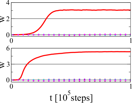
In Fig. 4, the evolution of the synaptic weights is presented as a function of time. In this case $b$ has been kept constant at $b=0$. Learning stops when $<\dot{w}>=0$, but since the learning rule is a non-linear function of $x$, the exact final value of $w$ will vary for different transfer functions. In the case of a bimodal input distribution, as the one used in the linear discrimination task, both clouds of points can be sent close to the minima and the final values of $w$ are then very similar, regardless of the choice of transfer function (not shown here).

Finally, we apply the rules to the non-linear bars problem. Here we follow the procedure of [15], where, in a grid of $L\times L$ inputs, each pixel can take two values, one for low intensity and one of high intensity. Each bar consists of a complete row or a complete column of high intensity pixels, and each possible bar is drawn independently with a probability $p=1/L$. At the intersection of a horizontal and vertical bar, the intensity is the same as if only one bar were present, which makes the problem non-linear. The neuron is then presented, at each training step, a new input drawn under the prescribed rules and after each step the evolution of the synaptic weights is updated. The bias $b$ in the model can either be adjusted as in [15] by, $\dot{b}\propto(y-p)$, or by maximal entropy intrinsic adaption, as described in [13], without mayor differences.

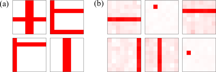
Figure 5: (a) Some random training examples for the non-linear bars problem. (b) Graphical representation of the typical weight vectors learnt by the neuron in distinct training runs.

Since the selectivity to a given pattern is given by the value of the scalar product $\bar{y}_{inputs}\cdot\bar{w}$, one can either compute the output activity $y$ to see to which pattern the neuron is selective in the end, or just do an intensity plot of the weights, since the maximal selectivity corresponds to $\bar{w}\propto\bar{y}_{inputs}$. In Fig. 5 a typical set of inputs is presented, together with a typical set of learnt neural weights for different realizations in a single neuron training. We see how a neuron is able to become selective to individual bars or to single points (the independent components in this problem). To check that the neuron can learn single bars, even when such a bar is never presented to the neuron in isolation as a stimulus, we also trained the neuron with a random pair of bars, one horizontal and one vertical, obtaining similar results. The neuron can learn to fire in response to a single bar, even when that bar was never presented in isolation.

3 Discussion and Concluding Remarks

The implementation of the stationarity principle in terms of the Fisher information, presented in [13] and here discussed, results in a set of Hebbian self-limiting rules for synaptic plasticity. The sensitivity of the rule to higher moments of the input probability distribution, makes it suitable for applications in independent component analysis. Furthermore, the learning rule derived is robust with respect to the choice of transfer function $g(x)$, a requirement for biological plausibility.

In upcoming work, we study the dependence of the steady state solutions of the neuron and their stability with respect to the moments of the input distribution. The numerical finding of independent component analysis in the bars problem is then justified. We will also study how a network of neurons can be trained using the same rules for all weights, feed-forward and lateral, and how clusters of input selectivity to different bars emerge in a self organized way.

References

- [1] Donald Olding Hebb. The organization of behavior: A neuropsychological theory. Psychology Press, 2002.
- [2] Elie L Bienenstock, Leon N Cooper, and Paul W Munro. Theory for the development of neuron selectivity: orientation specificity and binocular interaction in visual cortex. The Journal of Neuroscience, 2(1):32–48, 1982.
- [3] Erkki Oja. The nonlinear pca learning rule in independent component analysis. Neurocomputing, 17(1):25–45, 1997.
- [4] Geoffrey J Goodhill and Harry G Barrow. The role of weight normalization in competitive learning. Neural Computation, 6(2):255–269, 1994.
- [5] Terry Elliott. An analysis of synaptic normalization in a general class of hebbian models. Neural Computation, 15(4):937–963, 2003.
- [6] Teuvo Kohonen. Self-organization and associative memory. Self-Organization and Associative Memory, 100 figs. XV, 312 pages.. Springer-Verlag Berlin Heidelberg New York. Also Springer Series in Information Sciences, volume 8, 1, 1988.
- [7] C. Gros. Complex and adaptive dynamical systems: A primer. Springer Verlag, 2010.
- [8] Claudius Gros. Generating functionals for guided self-organization. In M. Prokopenko, editor, Guided Self-Organization: Inception, pages 53–66. Springer, 2014.
- [9] Gregoire Nicolis and Ilya Prigogine. Self-organization in nonequilibrium systems, volume 191977. Wiley, New York, 1977.
- [10] Jochen Triesch. Synergies between intrinsic and synaptic plasticity mechanisms. Neural Computation, 19(4):885–909, 2007.
- [11] Martin Stemmler and Christof Koch. How voltage-dependent conductances can adapt to maximize the information encoded by neuronal firing rate. Nature neuroscience, 2(6):521–527, 1999.
- [12] Dimitrije Marković and Claudius Gros. Intrinsic adaptation in autonomous recurrent neural networks. Neural Computation, 24(2):523–540, 2012.
- [13] Rodrigo Echeveste and Claudius Gros. Generating functionals for computational intelligence: The fisher information as an objective function for self-limiting hebbian learning rules. Computational Intelligence, 1:1, 2014.
- [14] Marcel Reginatto. Derivation of the equations of nonrelativistic quantum mechanics using the principle of minimum fisher information. Physical Review A, 58:1775–1778, 1998.
- [15] Peter Földiak. Forming sparse representations by local anti-hebbian learning. Biological cybernetics, 64(2):165–170, 1990.