Locations of stationary/periodic solutions in mean motion resonances according to properties of dust grains

Abstract

The equations of secular evolution for dust grains in mean motion resonances with a planet are solved for stationary points. This is done including both Poynting–Robertson effect and stellar wind. The solutions are stationary in semimajor axis, eccentricity, and resonant angle, but allow the pericentre to advance. The semimajor axis of stationary solutions can be slightly shifted from the exact resonant value. The periodicity of the stationary solutions in a reference frame orbiting with the planet is analytically proved. The existence of periodic solutions in mean motion resonances means that analytical theory enables for dust particles also infinitely long capture times. The stationary solutions are periodic motions to which the eccentricity asymptotically approaches and around which the libration occurs.

Using numerical integration of equation of motion are successfully found initial conditions corresponding to the stationary solutions. Numerically and analytically determined shifts of the semimajor axis form the exact resonance for the stationary solutions are in excellent agreement.

The stationary solutions can be plotted by locations of pericenters in the reference frame orbiting with the planet. The pericenters are distributed in the space according to properties of dust particles.

1 Introduction

A lenticular cloud of dust centered on the Sun with its main axis lying in the ecliptic plane creates well known zodiacal light. Discoveries and improving observations of debris disks around main-sequence stars (e.g. Holland et al., 1998; Debes, Weinberger & Kuchner, 2009; Schneider et al., 2014; Lagrange et al., 2016) motivate to understand better the dynamics of the dust particles in such environments. Sharp inner edges, clumps and asymmetries observed in the debris disks are commonly interpreted as signatures of a planet created in earlier stages of the disk evolution and located near or within the disks (e.g. Wyatt, 2003; Kuchner & Holman, 2003; Stark & Kuchner, 2009; Rodigas, Malhotra & Hinz, 2014). Such a planet can gravitationally capture the dust particles in the so called mean motion resonances (MMRs) and change the morphology of the disk.

Mean motion resonances occur when a ratio of orbital periods of the dust particle and the planet is near a ratio of two small natural numbers. The MMRs in a circular restricted three-body problem (CRTBP) with a stellar electromagnetic radiation and a stellar wind include numerous aspects which are directly applicable to astrophysical systems, ranging from the resonant dust ring close to the Earth’s orbit (e.g. Jackson & Zook, 1989; Dermott et al., 1994; Reach et al., 1995; Reach, 2010; Pástor, 2014b) through dust in the Edgeworth–Kuiper belt zone (e.g. Liou & Zook, 1999; Moro-Martín & Malhotra, 2002; Holmes et al., 2003; Kuchner & Stark, 2010) to structures observed in debris disks (e.g. Kuchner & Holman, 2003; Stark & Kuchner, 2008; Shannon, Mustill & Wyatt, 2015). Analytical results can be applied into semi-analytic models of resonant dust just to improve computation speed of resonant disk patterns (e.g. Wyatt, 2003; Kuchner & Holman, 2003; Stark & Kuchner, 2009; Rodigas et al., 2014; Shannon et al., 2015).

In this work we show that the CRTBP with radiation comprises also periodic solutions for the motion of the dust particle in an exterior MMR (the orbital period of the dust particle is larger than the orbital period of the planet in the exterior MMRs). The periodic solutions exist at “universal eccentricities” found by Beaugé & Ferraz-Mello (1994). The eccentricity of dust orbit during a capture in the exterior MMR approaches the universal eccentricity (e.g. Liou & Zook, 1997; Klačka et al., 2008; Stark & Kuchner, 2009). If such periodic solutions exist, then maximal capture times for the dust particles in the exterior MMRs should be infinite.

Using adiabatic invariant theory Gomes (1995) found a criterion determining whether the libration amplitude increases or decreases for dissipative forces which lead to an evolution of the eccentricity characterised with asymptotic approach of the eccentricity to the universal eccentricity. Results of averaged theory in Gomes (1995) showed that the libration amplitude must increase for the dust particles in all exterior resonances in the planar CRTBP with the Poynting–Robertson (PR) effect. Gomes (1995) results allow also the existence of the periodic solutions.

Periodic solutions in 1/1 resonance were already found to exist (Liou, Zook & Jackson, 1995; Pástor, 2014b). The existence of secularly stationary solutions in the vicinity of the triangular Lagrangian equilibrium points in spatial-circular, planar-elliptic and spatial-elliptic restricted three-body problem with the PR effect was recently confirmed in Lhotka & Celletti (2015).

The content of this paper is the following. In Section 2, are presented averaged resonant equations for the MMRs in the planar CRTBP with arbitrary non-gravitational effects for which secular theory can be applied (general case). In Section 3, are determined conditions for the stationary points in the general case. In Section 4, is shown that for astrophysical systems with rotational symmetry an evolution during the stationary solution in the MMR is always periodic. In Section 5, are derived the conditions for the stationary points when the non-gravitational effects are the PR effect and the radial stellar wind. In Section 6, we determine the stationary solutions for the considered non-gravitational effects, we discuss properties of the solutions and present pericenters of the orbits corresponding to the stationary solutions in a reference frame orbiting with the Earth. Conclusions are drawn in Section 7.

2 Averaged resonant equations for dust particle influenced by non-gravitational effects

Orbital evolution in a dynamical system is often averaged over a period of the dynamical system (secular framework). The secular framework also enables define a stationarity. In the secular framework the stationarity is obtained if one or more orbital elements remain constant after the averaging process. In the MMRs the semimajor axis of the particle orbit is also secularly stationary after the averaging over an libration period. In what follows the word secularly before the stationary will be omitted. A dust particle can be captured in an MMR with a planet in the planar CRTBP and simultaneously be affected by non-gravitational effects. In the general case secular variations of a particle orbit, caused by the non-gravitational effects, can depend on spatial orientation of the orbit. In this case resonant equations averaged over a synodic period have form (Pástor, 2014a):

$$\frac{dk}{dt}={} \frac{\alpha}{L}\frac{\partial R}{\partial h}-h\frac{d\sigma_{1}}{dt}-\frac{k\alpha}{L(1+\alpha)}\frac{dL}{dt}-\frac{k\alpha}{Le^{2}}\left\langle P_{2}\right\rangle-h\left\langle Q_{2}\right\rangle~{},$$

$$\frac{dh}{dt}={} -\frac{\alpha}{L}\frac{\partial R}{\partial k}+k\frac{d\sigma_{1}}{dt}-\frac{h\alpha}{L(1+\alpha)}\frac{dL}{dt}$$

$$-\frac{h\alpha}{Le^{2}}\left\langle P_{2}\right\rangle+k\left\langle Q_{2}\right\rangle~{},$$

$$\frac{dL}{dt}={} s\left(h\frac{\partial R}{\partial k}-k\frac{\partial R}{\partial h}\right)+\left\langle P_{1}\right\rangle~{},$$

$$\frac{d\sigma_{1}}{dt}={} \frac{p+q}{q}n_{\text{P}}-sn+\frac{2sa}{L}\frac{\partial R}{\partial^{\star}a}$$

$$-\frac{\alpha s}{L(1+\alpha)}\left(k\frac{\partial R}{\partial k}+h\frac{\partial R}{\partial h}\right)+s\left\langle Q_{1}\right\rangle~{}.$$ (1)

Here, $k$ $=$ $e\cos\sigma$ and $h$ $=$ $e\sin\sigma$ are the non-canonical resonant variables, $e$ is the eccentricity of the particle orbit, and $\sigma$ is the resonant angular variable $\sigma$ $=$ $\psi/q-\tilde{\omega}$. The expression for the resonant angular variable contains: $\psi$ $=$ $(p+q)\lambda_{\text{P}}-p\lambda$, two integers $p$ and $q$, the mean longitude $\lambda$, and the longitude of pericenter $\tilde{\omega}$. The subscript P is used for quantities belonging to the planet. $\alpha$ $=$ $\sqrt{1-e^{2}}$, $s$ $=$ $p/q$, and $\sigma_{1}$ $=$ $\psi/q-\tilde{\omega}_{\text{P}}$. $R$ is the disturbing function of the planar CRTBP. $L$ $=$ $\sqrt{\mu a}$, where, $\mu$ $=$ $G_{0}M_{\star}$, $G_{0}$ is the gravitational constant, $M_{\star}$ is the mass of the star, and $a$ is the semimajor axis of the particle orbit. $n$ $=$ $\sqrt{\mu/a^{3}}$ is the mean motion of the particle. $\partial^{\star}a$ denotes the partial derivative with respect to the semimajor axis calculated with an assumption that the mean motion of the particle $n$ is not a function of the semimajor axis (see e.g. Danby, 1988). We use angle $\sigma_{\text{b}}$ defined so that the mean anomaly $M$ can be computed from $M$ $=$ $nt$ $+$ $\sigma_{\text{b}}$ (Bate, Mueller & White, 1971). In this case the following relations hold between the averaged partial derivatives of the disturbing function (Pástor, 2014a)

$$\frac{\partial R}{\partial\sigma_{\text{b}}} =-s\frac{\partial R}{\partial\sigma}~{},$$

$$\frac{\partial R}{\partial\tilde{\omega}} =-\frac{p+q}{q}\frac{\partial R}{\partial\sigma}~{},$$

$$\frac{\partial R}{\partial\sigma} =k\frac{\partial R}{\partial h}-h\frac{\partial R}{\partial k}~{},$$

$$e\frac{\partial R}{\partial e} =k\frac{\partial R}{\partial k}+h\frac{\partial R}{\partial h}~{}.$$ (2)

From the definitions after Eqs. (2) we have $\sigma$ $=$ $\psi/q-\tilde{\omega}$ and $\sigma_{1}$ $=$ $\psi/q-\tilde{\omega}_{\text{P}}$. Therefore, the last equation in Eqs. (2) reads

$$\frac{d\sigma_{1}}{dt}=\frac{d\sigma}{dt}+\frac{d\tilde{\omega}}{dt}~{},$$ (3)

where we have used the fact that $\tilde{\omega}_{\text{P}}$ $=$ 0 in the CRTBP. When we again use the definitions after Eqs. (2) for $L$ $=$ $\sqrt{\mu a}$, $k$ $=$ $e\cos\sigma$ and $h$ $=$ $e\sin\sigma$ we can obtain, using some analytic manipulations, the following useful relations

$$\frac{da}{dt} =\frac{2a}{L}\frac{dL}{dt}~{},$$

$$\frac{de}{dt} =\frac{1}{e}\left(k\frac{dk}{dt}+h\frac{dh}{dt}\right)~{},$$

$$\frac{d\sigma}{dt} =\frac{1}{e^{2}}\left(k\frac{dh}{dt}-h\frac{dk}{dt}\right)~{}.$$ (4)

Eqs. (2), Eq. (3) and Eqs. (2) can be used in order to rewrite Eqs. (2) as follows

$$\frac{da}{dt}={} \frac{2a}{L}\left(-s\frac{\partial R}{\partial\sigma}+\left\langle P_{1}\right\rangle\right)~{},$$

$$\frac{de}{dt}={} \frac{\alpha}{Le}\left\{\left[1+s\left(1-\alpha\right)\right]\frac{\partial R}{\partial\sigma}-\left(1-\alpha\right)\left\langle P_{1}\right\rangle-\left\langle P_{2}\right\rangle\right\}~{},$$

$$\frac{d\tilde{\omega}}{dt}={} \frac{\alpha}{Le}\frac{\partial R}{\partial e}-\left\langle Q_{2}\right\rangle~{},$$

$$\frac{d\sigma}{dt}={} \frac{p+q}{q}n_{\text{P}}-sn-\frac{\alpha}{Le}\left[1+s\left(1-\alpha\right)\right]\frac{\partial R}{\partial e}$$

$$+\frac{2sa}{L}\frac{\partial R}{\partial^{\star}a}+s\left\langle Q_{1}\right\rangle+\left\langle Q_{2}\right\rangle~{}.$$ (5)

The system given by Eqs. (2) enables to study the secular orbital evolution of the dust particle captured in the specific MMR given by the resonant numbers $p$ and $q$ under the action of the non-gravitational effects. The expression of Eqs. (2) using the orbital elements and the resonant angular variable, given by Eqs. (2), will be useful for a determination of properties of the stationary solutions as we will see later. For the averaged non-conservative terms $\langle Q_{i}\rangle$ and $\langle P_{i}\rangle$, $i$ $=$ 1, 2 hold (Pástor, 2014a)

$$\left\langle Q_{1}\right\rangle =-\left\langle\frac{d\tilde{\omega}}{dt}\right\rangle_{\text{EF}}-\left\langle\frac{d\sigma_{\text{b}}}{dt}+t\frac{dn}{dt}\right\rangle_{\text{EF}}~{},$$

$$\left\langle Q_{2}\right\rangle =-\left\langle\frac{d\tilde{\omega}}{dt}\right\rangle_{\text{EF}}~{},$$

$$\left\langle P_{1}\right\rangle =\frac{na}{2}\left\langle\frac{da}{dt}\right\rangle_{\text{EF}}~{},$$

$$\left\langle P_{2}\right\rangle =-\frac{na(1-\alpha)}{2}\left\langle\frac{da}{dt}\right\rangle_{\text{EF}}-\frac{na^{2}e}{\alpha}\left\langle\frac{de}{dt}\right\rangle_{\text{EF}}~{},$$ (6)

where $\langle da/dt\rangle_{\text{EF}}$, $\langle de/dt\rangle_{\text{EF}}$, $\langle d\tilde{\omega}/dt\rangle_{\text{EF}}$, and $\langle d\sigma_{\text{b}}/dt$ $+$ $t$ $dn/dt\rangle_{\text{EF}}$ are caused by the non-gravitational effects only. The averaged values on the right-hand sides in Eqs. (2) can be obtained using the Gaussian perturbation equations of celestial mechanics (e.g. Danby, 1988). Their specific values for the PR effect and the radial stellar wind will be shown later. The equations in this section are derived for the general case.

3 Conditions for stationary points

The stationary points in the $kh$ plane are determined by

$$\frac{dk}{dt}=\frac{dh}{dt}=0~{}.$$ (7)

If Eqs. (7) hold in a case without the non-gravitational effects (conservative problem), then they affect also the evolution of the semimajor axis. This is due to the fact that the condition $de/dt$ $=$ 0 implies $da/dt$ $=$ 0. This can be most easily seen if we calculate time derivative of the eccentricity averaged over the synodic period using the first two equations in Eqs. (2) and the last two equations in Eqs. (2) (see also Eq. 17 in Pástor 2014a)

$$\frac{de}{dt}={} \frac{\alpha}{2ae}\left(\alpha-\frac{p+q}{p}\right)\frac{da}{dt}$$

$$+\frac{\alpha}{2ae}\left(\frac{p+q}{p}-\alpha\right)\left\langle\frac{da}{dt}\right\rangle_{\text{EF}}+\left\langle\frac{de}{dt}\right\rangle_{\text{EF}}~{}.$$ (8)

In the conservative problem Eq. (3) gives for $de/dt$ $=$ 0 that $da/dt$ $=$ 0 or $dL/dt$ $=$ 0 (see also Beaugé & Ferraz-Mello, 1994). Eq. (3) shows that in the case with the non-gravitational effects $de/dt$ $=$ 0 is not sufficient for $dL/dt$ $=$ 0, in general. We are interested in the stationary solutions of the system of equations given by Eqs. (2) restricted by the same conditions as in the conservative problem. If we add the condition $dL/dt$ $=$ 0 to the conditions in Eqs. (7), then the semimajor axis will be also stationary similarly as in the conservative problem at the stationary points in the $kh$ plane. The condition $dL/dt$ $=$ 0 is necessary for the periodicity of the stationary solutions as we will see later. Hence, the stationary points will be determined by the substitution of the following three equations into Eqs. (2)

$$\frac{dk}{dt}=\frac{dh}{dt}=\frac{dL}{dt}=0~{}.$$ (9)

Eqs. (9) were used also in Beaugé & Ferraz-Mello (1993) and Šidlichovský & Nesvorný (1994).

The substitution of Eqs. (9) into Eqs. (2) leads to the conditions

$$\left\langle P_{1}\right\rangle-s\left\langle P_{2}\right\rangle =0~{},$$

$$e\frac{\partial R}{\partial e}=k\frac{\partial R}{\partial k}+h\frac{\partial R}{\partial h} =\frac{Le^{2}}{\alpha}\left(\frac{d\sigma_{1}}{dt}+\left\langle Q_{2}\right\rangle\right)~{},$$

$$\frac{\partial R}{\partial\sigma}=k\frac{\partial R}{\partial h}-h\frac{\partial R}{\partial k} =\left\langle P_{2}\right\rangle~{}.$$ (10)

Eqs. (9) are equivalent with

$$\frac{da}{dt}=\frac{de}{dt}=\frac{d\sigma}{dt}=0~{},$$ (11)

as can be seen from Eqs. (2). The semimajor axis and the position of the libration center in the $kh$ plane are stationary in the sought for stationary points.

4 Periodicity of evolutions corresponding to stationary solutions in resonances

In the exact resonance the averaged mean motion of the particle and the mean motion of the planet have a ratio that is exactly equal to the ratio of two natural numbers. The periodicity of evolutions corresponding to the stationary solutions in the exact resonances with fixed longitude of pericenter was already showed in Pástor (2014a). In this work we take into account the possibility that the longitude of pericenter can be variable. Influence of the variable longitude of pericenter on the periodicity of the evolutions during the stationary solutions will be determined. Beside the variable longitude of pericenter in this work we consider also non-exact resonances. In this section, the symbols used denote the un-averaged quantities. We assume that the physical parameters of the planar CRTBP with the non-gravitational effects do not change during the synodic period. In our case, the un-averaged resonant angular variable is

$$\sigma=\frac{p+q}{q}\lambda_{\text{P}}-s\lambda-\tilde{\omega}~{},$$ (12)

with the mean longitude

$$\lambda=M+\tilde{\omega}=nt+\sigma_{\text{b}}+\tilde{\omega}~{}.$$ (13)

For the time derivative of the mean longitude in Eqs. (13) we obtain

$$\frac{d\lambda}{dt}=n+\frac{d\sigma_{\text{b}}}{dt}+t\frac{dn}{dt}+\frac{d\tilde{\omega}}{dt}~{}.$$ (14)

Using the previous equation we obtain for the time derivative of $\sigma$ in Eq. (12)

$$\frac{d\sigma}{dt}=\frac{p+q}{q}n_{\text{P}}-sn-s\left(\frac{d\sigma_{\text{b}}}{dt}+t\frac{dn}{dt}+\frac{d\tilde{\omega}}{dt}\right)-\frac{d\tilde{\omega}}{dt}~{}.$$ (15)

Let the motion be stationary according to the conditions in Eqs. (11). Eq. (15) can be averaged over the synodic period. If we use the last condition in Eqs. (11) for the stationarity of the resonant angular variable in the result of averaging, we obtain

$$\frac{p+q}{q}n_{\text{P}}-\frac{s}{T_{\text{S}}}\int_{0}^{T_{\text{S}}}n~{}dt-\frac{p+q}{q}\frac{1}{T_{\text{S}}}\int_{0}^{T_{\text{S}}}\frac{d\tilde{\omega}}{dt}dt$$

$$-\frac{s}{T_{\text{S}}}\int_{0}^{T_{\text{S}}}\left(\frac{d\sigma_{\text{b}}}{dt}+t\frac{dn}{dt}\right)dt=0~{}.$$ (16)

In Pástor (2014a) only the exact resonances were considered. The condition $n_{\text{P}}~{}(p+q)/p$ $=$ $(1/T_{\text{S}})$ $\int_{0}^{T_{\text{S}}}$ $n~{}dt$ valid for the exact resonances may not be valid for the non-exact resonances. Therefore, the first two terms in Eq. (4) may not cancel each other as in the case for the exact resonances.

The periodicity of evolution corresponding to the stationary solution in Pástor (2014a) was demostrated for the non-gravitational effects which include an interstellar wind. For the star moving through a cloud of an interstellar matter the interstellar wind is monodirectional (for details see Baines, Williams & Asebiomo, 1965). The monodirectional character of the interstellar wind enables only the stationary solutions for which the longitude of pericenter is stationary. The third term in Eq. (4) is caused by the variability (instationarity) of the longitude of pericenter and in Pástor (2014a) was equal to zero.

Figure 1: Evolution of a dust particle with $R_{\text{d}}$ $=$ 5 $\mu$m, $\varrho$ $=$ 2 g/cm³, and $\bar{Q}^{\prime}_{\text{pr}}$ $=$ 1 captured in an exterior mean motion 6/5 orbital resonance in the planar CRTBP with the PR effect and the radial solar wind which comprises the Earth and the Sun as the two main bodies. Depicted evolving parameters are described in the text. The dashed line in the second plot shows the asymptotic value of the eccentricity. The dashed line in the $kh$ plane indicates the values of $e$ and $\sigma$ that lead to collisions of the planet with the particle. All evolving parameters are averaged over the synodic period.

Table 1: The universal eccentricity (the first equation in Eqs. 5) for several exterior resonances. The eccentricities implicate from Eqs. (9) when the non-gravitational effects are the PR effect and the radial stellar wind.

1${}^{\text{st}}$ order		2${}^{\text{nd}}$ order		3${}^{\text{rd}}$ order
$p/(p+q)$	universal $e$	$p/(p+q)$	universal $e$	$p/(p+q)$	universal $e$
9/8	0.1986	9/7	0.2904	8/5	0.3972
8/7	0.2115	7/5	0.3362	7/4	0.4331
7/6	0.2273	5/3	0.4140	5/2	0.5505
6/5	0.2472	3/1	0.5993	4/1	0.6654
5/4	0.2736
4/3	0.3108
3/2	0.3690
2/1	0.4812

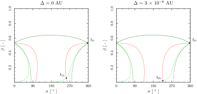
Figure 2: Solutions of the conditions for the stationary points in the planar CRTBP with radiation (Eqs. 5). Solutions of the second equation, determined at the universal eccentricity, are depicted with red curves. Similarly solutions of the third equation are depicted with green curves. Dust particles are captured in an exterior 6/5 MMR with the Earth in a circular orbit around the Sun. In the left plot is $\Delta$ $=$ 0 used and the right plot was obtained using $\Delta$ $=$ 3 $\times$ 10^-6 AU. Black circles indicate intersections of red and green lines representing solutions of the system given by Eqs. (5).

Figure 3: Evolution of orbital parameters averaged over the synodic period obtained from numerical integration of the equation of motion (Eq. 5) close to the stationary point $\text{I}_{2\text{b}}$ depicted in Fig. 2. A dust particle with $\beta$ $=$ 0.02027611 and $\bar{Q}^{\prime}_{\text{pr}}$ $=$ 1 is captured in an exterior mean motion 6/5 orbital resonance with the Earth in a circular orbit around the Sun under the action of the PR effect and the radial solar wind. The stationary solution occurs in a non-exact MMR. Un-averaged evolution during the first 30 years can be seen in Fig. 4.

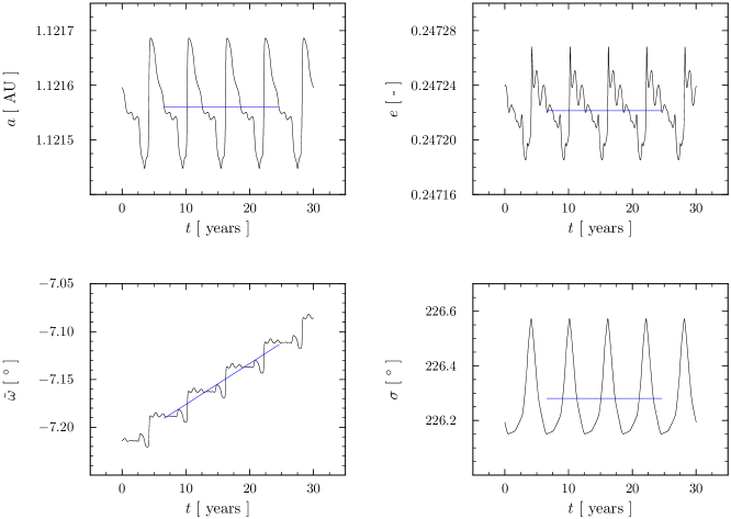
Figure 4: Evolution of osculating orbital parameters during initial 30 years of the evolution depicted in Fig. 3 (black line). For the sake of comparison also the evolution of orbital parameters averaged over the synodic period is shown (blue line). The averaged evolution is created only by four points placed in the middle of a given averaged synodic period. Scales on vertical axes are different from the scales in Fig. 3 in order to show full evolution of osculating $a$, $e$ and $\sigma$ during the synodic period.

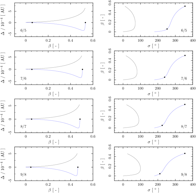
Figure 5: Stationary solutions found from Eqs. (5). Dependencies of the shift from the exact resonance $\Delta$ on $\beta$ (left column) and dependencies of $\beta$ on the resonant angular variable $\sigma$ (right column) are shown for 6/5, 7/6, 8/7 and 9/8 exterior MMRs in a circular Sun-Earth-dust problem with the PR effect and the radial solar wind. Equal color in a given row for a given resonance corresponds to the same sets of the stationary solutions. The semimajor axis of the solutions can be computed as $a$ $=$ $a_{\text{r}}$ $+$ $\Delta$. The stationary solutions in the exact resonances are marked with black circles. The stationary eccentricity is equal to the universal eccentricity.

Figure 6: Pericenters of orbits corresponding to the stationary solutions shown in the reference frame orbiting with the Earth for dust particles captured in 6/5, 7/6, 8/7 and 9/8 exterior mean motion orbital resonances in a circular Sun-Earth-dust problem with radiation. The eccentricity of orbits is equal to the universal eccentricity. Intervals for $\tilde{\omega}$ are calculated from $\sigma$ depicted in the right column of Fig. 5 (see text). $\beta_{\text{max}}$ is maximal $\beta$ at which the stationary solution exists and $\beta_{\text{max}}$ belongs to the 6/5 resonance ($\beta_{\text{max}}$ $=$ 0.532394).

Eq. (14) can also be averaged over the synodic period. If we substitute Eq. (4) in the averaged Eq. (14), then we obtain

$$\frac{1}{T_{\text{S}}}\int_{0}^{T_{\text{S}}}\frac{d\lambda}{dt}dt=\frac{p+q}{p}n_{\text{P}}-\frac{q}{p}\frac{1}{T_{\text{S}}}\int_{0}^{T_{\text{S}}}\frac{d\tilde{\omega}}{dt}dt~{}.$$ (17)

In the equation above we can see that the difference between mean longitudes after the synodic period $T_{\text{S}}$ depends on the synodic period and on the averaged time derivative of the longitude of pericenter. In what follows we determine a relation between these two variables. Eqs. (2) were obtained by the averaging over the synodic period using a cyclic angular variable $\sigma_{2}$ as the integration variable. $\sigma_{2}$ is defined (see e.g. Šidlichovský & Nesvorný, 1994) as follows

$$\sigma_{2}=\frac{\lambda-\lambda_{\text{P}}}{q}~{}.$$ (18)

The difference between $\sigma_{2}$ at time zero and $\sigma_{2}$ after one synodic period $T_{\text{S}}$ is equal to $2\pi$. Implicit differentiation of $\sigma_{2}$ defined in Eq. (18) yields

$$d\sigma_{2}=\frac{1}{q}\left(n~{}dt+t~{}dn+d\sigma_{\text{b}}+d\tilde{\omega}-n_{\text{P}}~{}dt\right)~{}.$$ (19)

The last equation can be integrated over the synodic period

$$2\pi={} \frac{1}{q}\biggl{[}\int_{0}^{T_{\text{S}}}n~{}dt+\int_{0}^{T_{\text{S}}}\left(\frac{d\sigma_{\text{b}}}{dt}+t~{}\frac{dn}{dt}\right)dt$$

$$+\int_{0}^{T_{\text{S}}}\frac{d\tilde{\omega}}{dt}dt-n_{\text{P}}~{}T_{\text{S}}\biggr{]}~{}.$$ (20)

Substitution Eq. (4) into Eq. (4) yields the sought for relation between the synodic period and the averaged time derivative of the longitude of pericenter

$$2\pi p=n_{\text{P}}T_{\text{S}}-\int_{0}^{T_{\text{S}}}\frac{d\tilde{\omega}}{dt}dt~{}.$$ (21)

The difference between mean anomalies after one synodic period can be obtained using

$$\frac{1}{T_{\text{S}}}\int_{0}^{T_{\text{S}}}\frac{d\lambda}{dt}dt=\frac{1}{T_{\text{S}}}\int_{0}^{T_{\text{S}}}\frac{dM}{dt}dt+\frac{1}{T_{\text{S}}}\int_{0}^{T_{\text{S}}}\frac{d\tilde{\omega}}{dt}dt$$ (22)

and Eq. (21) in Eq. (17). We obtain

$$\frac{1}{T_{\text{S}}}\int_{0}^{T_{\text{S}}}\frac{dM}{dt}dt=\left(p+q\right)\frac{2\pi}{T_{\text{S}}}~{}.$$ (23)

The last equation finally implies

$$M(T_{\text{S}})-M(0)=\left(p+q\right)2\pi~{}.$$ (24)

Now, we rewrite Eq. (21) as follows

$$\tilde{\omega}(0)-\lambda_{\text{P}}(0)=\tilde{\omega}(T_{\text{S}})-\lambda_{\text{P}}(T_{\text{S}})+2\pi p~{},$$ (25)

where we have used the identity $\lambda_{\text{P}}(T_{\text{S}})$ $-$ $\lambda_{\text{P}}(0)$ $=$ $n_{\text{P}}T_{\text{S}}$. Eq. (25) shows that a difference in the angle between the planet and the pericenter of the particle orbit after the synodic period is an integer multiplied by $2\pi$. Eq. (25) takes into account the arbitrary variability of the longitude of pericenter. Eq. (24) gives that after the synodic period the particle is in the same position on the orbit as in the time zero. The first two equations in Eqs. (11) ensure that after the synodic period the semimajor axis and the eccentricity are the same as in the time zero. On the basis of Eqs. (11), Eq. (24) and Eq. (25) we can draw the following conclusions for the evolution during the stationary solution in the resonance. If the secular time derivatives of the orbital elements caused by the non-gravitational effects (non-gravitational secular variations) do not depend on the longitude of pericenter, then the evolution will be repeated after the synodic period (the motion of the dust particle is periodic). The non-gravitational secular variations do not depend on the longitude of pericenter in astrophysical systems with rotational symmetry (Appendix A). In the cases when the non-gravitational secular variations depend on the longitude of pericenter the variation of the longitude of pericenter after one synodic period can cancel the periodicity.

5 Conditions for stationary points with PR effect and radial stellar wind

Let us consider a star which produces an electromagnetic radiation and a radial stellar wind with one planet in a circular orbit. In astrophysical modelling of the orbital evolution of dust grains it is often assumed that a spherical particle can be used as an approximation to real, the arbitrarily shaped, particle. The force associated with the action of the electromagnetic radiation on the moving the spherical dust particle is the PR effect (Poynting, 1904; Robertson, 1937; Klačka, 2004; Klačka et al., 2014). The stellar wind also affects the dynamics of the dust particles. A relativistically covariant equation of motion of the dust particle caused by a parallel beam of corpuscules impinging on the dust particle was derived in Klačka et al. (2012). On the basis of the mentioned papers we obtain the following equation of motion for the spherical dust particle in a reference frame associated with the star in accuracy to first order in $v/c$ ($v$ is the speed of the dust particle with respect to the star and $c$ is the speed of light in vacuum), first order in $u/c$ ($u$ is the speed of the stellar wind with respect to the star) and first order in $v/u$

$$\frac{d\vec{v}}{dt}={} -\frac{\mu}{r^{2}}\left(1-\beta\right)\vec{e}_{\text{R}}-\frac{G_{0}M_{\text{P}}}{|\vec{r}-\vec{r}_{\text{P}}|^{3}}\left(\vec{r}-\vec{r}_{\text{P}}\right)-\frac{G_{0}M_{\text{P}}}{r_{\text{P}}^{3}}\vec{r}_{\text{P}}$$

$$-\beta\frac{\mu}{r^{2}}\left(1+\frac{\eta}{\bar{Q}^{\prime}_{\text{pr}}}\right)\left(\frac{\vec{v}\cdot\vec{e}_{\text{R}}}{c}\vec{e}_{\text{R}}+\frac{\vec{v}}{c}\right)~{},$$ (26)

where $r$ is the radial distance between the star and the dust particle, $\vec{e}_{\text{R}}$ is the unit vector directed from the star to the particle, $\vec{v}$ the velocity of the particle with respect to the star, $M_{\text{P}}$ is the mass of the planet, $\vec{r}_{\text{P}}$ is the position vector of the planet with respect to the star, and $r_{\text{P}}$ $=$ $|\vec{r}_{\text{P}}|$. The parameter $\beta$ is defined as the ratio between the electromagnetic radiation pressure force and the gravitational force between the star and the particle at rest with respect to the star. For $\beta$ we have from its definition

$$\beta=\frac{3L_{\star}\bar{Q}^{\prime}_{\text{pr}}}{16\pi c\mu R_{\text{d}}\varrho}~{},$$ (27)

where $L_{\star}$ is the stellar luminosity, $\bar{Q}^{\prime}_{\text{pr}}$ is the dimensionless efficiency factor for the radiation pressure averaged over the stellar spectrum and calculated for the radial direction ($\bar{Q}^{\prime}_{\text{pr}}$ $=$ 1 for a perfectly absorbing sphere), $c$ is the speed of light in vacuum, and $R_{\text{d}}$ is the radius of the dust particle with mass density $\varrho$. $\eta$ is to the given accuracy the ratio of the stellar wind energy to the stellar electromagnetic radiation energy, both radiated per unit time

$$\eta=\frac{4\pi r^{2}u}{L_{\star}}\sum_{i=1}^{N}n_{\text{sw}~{}i}m_{\text{sw}~{}i}c^{2}~{},$$ (28)

where $m_{\text{sw}~{}i}$ and $n_{\text{sw}~{}i}$, $i$ $=$ 1 to $N$, are the masses and concentrations of the stellar wind particles at a distance $r$ from the star ($u$ $=$ 450 km/s and $\eta$ $=$ 0.38 for the Sun, Klačka et al. 2012).

The orbital evolution will be given by the evolution of osculating orbital elements calculated for the case when a central acceleration is defined by the first Keplerian term in Eq. (5), namely $-\mu\left(1-\beta\right)\vec{e}_{\text{R}}/r^{2}$. The expressions in the previous sections which contain $L$ and $n$ must be modified for this central acceleration using a reduced mass of the star $M_{\star}(1-\beta)$. The modifying equations are $L$ $=$ $\sqrt{\mu(1-\beta)a}$ and $n$ $=$ $\sqrt{\mu(1-\beta)/a^{3}}$. Using the last term in Eq. (5) as a perturbation of the orbital motion we obtain from the Gaussian perturbation equations of celestial mechanics the following averaged values in Eqs. (2)

$$\left\langle\frac{da}{dt}\right\rangle_{\text{EF}}={} -\frac{\beta\mu}{ca\alpha^{3}}\left(1+\frac{\eta}{\bar{Q}^{\prime}_{\text{pr}}}\right)\left(2+3e^{2}\right)~{},$$

$$\left\langle\frac{de}{dt}\right\rangle_{\text{EF}}={} -\frac{\beta\mu}{2ca^{2}\alpha}\left(1+\frac{\eta}{\bar{Q}^{\prime}_{\text{pr}}}\right)5e~{},$$

$$\left\langle\frac{d\tilde{\omega}}{dt}\right\rangle_{\text{EF}}={} 0~{},$$

$$\left\langle\frac{d\sigma_{\text{b}}}{dt}+t\frac{dn}{dt}\right\rangle_{\text{EF}}={} 0~{}.$$ (29)

The substitution of Eqs. (5) into Eqs. (2) gives

$$\left\langle Q_{1}\right\rangle =0~{},$$

$$\left\langle Q_{2}\right\rangle =0~{},$$

$$\left\langle P_{1}\right\rangle =-\frac{\beta\mu n}{2c\alpha^{3}}\left(1+\frac{\eta}{\bar{Q}^{\prime}_{\text{pr}}}\right)\left(3e^{2}+2\right)~{},$$

$$\left\langle P_{2}\right\rangle =-\left\langle P_{1}\right\rangle-\frac{\beta\mu n}{c}\left(1+\frac{\eta}{\bar{Q}^{\prime}_{\text{pr}}}\right)~{}.$$ (30)

Now, we return to the conditions for the stationary points during a capture in the MMRs occurring in the planar CRTBP with non-gravitational effects given by Eqs. (3). The substitution of Eqs. (5) in Eqs. (3) yields for the PR effect and the radial solar wind

$$1-\frac{3e^{2}+2}{2\alpha^{3}}\frac{p+q}{p} =0~{},$$

$$\frac{\alpha}{Le}\left[1+s\left(1-\alpha\right)\right]\frac{\partial R}{\partial e} =\frac{p+q}{q}n_{\text{P}}-sn+\frac{2sa}{L}\frac{\partial R}{\partial^{\star}a}~{},$$

$$\frac{\partial R}{\partial\sigma} =-\frac{q}{p+q}\frac{\beta\mu n}{c}\left(1+\frac{\eta}{\bar{Q}^{\prime}_{\text{pr}}}\right)~{}.$$ (31)

For an interior resonance the first equation in Eqs. (5) does not have any solution. $p+q$ $<$ $p$ holds in an exterior resonance and the solution of the first equation in Eqs. (5) is the “universal eccentricity” (Beaugé & Ferraz-Mello, 1994; Liou & Zook, 1997). The universal eccentricities for several exterior resonances are in Table 1.

An example of the evolution approaching to the universal eccentricity is depicted in Fig. 1. The evolution is obtained from numerical solution of the equation of motion (Eq. 5) for a dust particle with $R_{\text{d}}$ $=$ 5 $\mu$m, $\varrho$ $=$ 2 g/cm³, and $\bar{Q}^{\prime}_{\text{pr}}$ $=$ 1 captured in an exterior mean motion 6/5 orbital resonance with the Earth in a circular orbit around the Sun under the action the PR effect and the radial solar wind. The depicted parameters are from left to right and from top to bottom, as follows: $a$ (semimajor axis), $e$ (eccentricity), $\tilde{\omega}$ (longitude of perihelion), $\sigma$ (resonant angular variable), $kh$ point, $k$ $=$ $e\cos\sigma$, $h$ $=$ $e\sin\sigma$, $L$ $=$ $\sqrt{\mu(1-\beta)a}$, and $\sigma_{1}$ $=$ $(p+q)\lambda_{\text{P}}/q$ $-$ $p\lambda/q$. Collisions of the particle with the planet occur on dashed lines in the $kh$ plane. The dashed lines cannot be crossed by the $kh$ point during the evolution in an MMR.

6 Stationary/periodic solutions

Stationary solutions can be found as intersections of solutions of the second and the third equation in Eqs. (5) at the universal eccentricity for one chosen semimajor axis and for one chosen longitude of pericenter. The semimajor axis will be given by a shift $\Delta$ from an exact resonant semimajor axis determined by the condition $a_{\text{r}}$ $=$ $a_{\text{P}}$ $(1-\beta)^{1/3}$ $[M_{\star}/(M_{\star}+M_{\text{P}})]^{1/3}$ $[p/(p+q)]^{2/3}$. From this definition we have $\Delta$ $=$ $a$ $-$ $a_{\text{r}}$. Solutions of the second equation (red line) and third equation (green line) in Eqs. (5) are depicted in Fig. 2. Collisions of the particle with the planet occur on curves depicted with dashed lines. Solved system comprises the Sun and the Earth as two main bodies in the planar CRTBP with radiation. The equations were solved for all dust particles with $\bar{Q}^{\prime}_{\text{pr}}$ $=$ 1 which can be in bound orbits around the Sun ($\beta$ $<$ 1) and are captured in the exterior mean motion 6/5 orbital resonance with the Earth. The eccentricity of particle orbit is equal to the universal eccentricity and the longitude of pericenter of particle orbit is equal to zero for both panels. In reality, the positions of the lines in Fig. 2 should not be depended on the longitude of pericenter (see Section 4). Depending on used numerical averaging method their positions can be found to be slightly depended on $\tilde{\omega}$. The left panel has $\Delta$ $=$ 0 and the right panel has $\Delta$ $=$ 3 $\times$ 10^-6 AU. As can be seen in Fig. 2 the positions of the green lines are not significantly dependent on $\Delta$ while the positions of the red lines are. Top boundaries for the collisions in Fig. 2 are obtained when an aphelion of the particle orbit is located on the planetary orbit. The value of $\beta_{\text{top}}$ on the boundaries can be calculated as

$$\beta_{\text{top}}=1-\frac{M_{\star}+M_{\text{P}}}{M_{\star}}\left(\frac{p+q}{p}\right)^{2}\left(\frac{1}{1+e_{\text{lim}}}-\frac{\Delta}{a_{\text{P}}}\right)^{3}~{},$$ (32)

where $e_{\text{lim}}$ is the universal eccentricity. Solutions of the third equation (green lines) for large values of $\beta$ are close to the collisions. At large $\beta$ strong gravitational pull from the planet is needed in order to compensate the influence caused by the PR effect and the solar wind (Eqs. 5). Very large values of $\beta$ are shown in Fig. 2 only for completeness of the depicted solutions since a capture of the dust particle in an MMR at these values of $\beta$ is complicated by strong perturbation from the non-gravitational effects. The stationary solutions are located in intersections of the red lines and the green lines in Fig. 2. The intersections are marked with black circles. Two intersections exist for each panel. The top intersections (subscript t) are located close to collisions while the bottom intersections are not.

Orbital evolution obtained from numerical solution of the equation of motion (Eq. 5) during a stationary solution is presented in Fig. 3. All evolving parameter are obtained from averaging over the synodic period (evolution of osculating orbital parameters during initial 30 years of this numerical solution can be seen in Fig. 4). The stationary evolution is found for the stationary point $\text{I}_{2\text{b}}$ depicted in Fig. 2. Numerically found $\Delta$ of the averaged semimajor axis is 3.0057 $\times$ 10^-6 AU. This is in an excellent agreement with value 3 $\times$ 10^-6 AU predicted by presented analytical theory for this dust particle (see Fig. 2). During the time of integration the longitude of pericenter increased by about 4.2419^∘. At greater resolution of vertical axes in Fig. 3 it is possible to see oscillations in the evolutions of $a$, $e$ and $\sigma$. This is caused by finite possibilities of the numerical integration. The stationary $e$ and $\sigma$ determined by the numerical solution of the equation of motion are found to be very sensitive on a precision of the numerical integration. Differences between the values of the stationary $e$ and $\sigma$ obtained from the presented analytical theory and the values obtained from the numerical integration can be caused also by limits of averaging used in the determination of the analytical values.

We searched the stationary solutions for exterior resonances 6/5, 7/6, 8/7 and 9/8 in a circular Sun-Earth-dust problem with the PR effect and the radial solar wind. We have chosen these exterior resonances since the orbits corresponding to the stationary solutions for exterior resonances of the first order ($q$ $=$ $-$ 1) with $p$ $<$ 6 reach close to or behind the orbit of Mars for particles with small $\beta$. We must note that the orbits corresponding to the stationary solutions for the considered exterior resonances at large $\beta$ ($\sim$ 0.5) can reach the orbit of Venus. The stationary solutions are shown in Fig. 5. Dependencies of $\Delta$ on $\beta$ are shown in the left column of the figure and dependencies of $\beta$ on $\sigma$ are shown in the right column of the figure. Equal color on both sides corresponds to equal set of the solutions. We will call these sets of the solutions branches. The bottom branches of the left-hand side plots begins at $\beta$ $=$ 0 and ends with the solution with $\Delta$ $=$ 0. The stationary solutions for the exact resonances are marked with black circles. The top branches of the left-hand side plots ends with minimal $\beta$ for which a crossing of collision curves occur if are all stationary $\Delta$ considered. Such a crossing is located in Fig. 2 close to the left and the right margins of both plots. The crossing of collision lines corresponds to such a particle on such an orbit that collision occurs during one orbit before and also after the pericenter of the particle orbit (in Keplerian approximation of the motion).

According to the results in Section 4 the angle between the planet and the pericenter of the particle orbit does not change after the synodic period. In Fig. 6 are shown pericenters of the stationary solutions in a reference frame orbiting with the Earth. The number of stationary branches in this reference frame is multiplied by $p$ $+$ $q$. This is caused by the periodicity of $\sigma$ with the period $2\pi$ and by the identity $\tilde{\omega}$ $=$ $-$ $q$ / $(p+q)$ $\sigma$ holding for the particle in pericenter and the planet located on the $x$-axis (Eq. 12). In the Fig. 6 we can see that the pericentes create a ring inside of Earth’s orbit. When the particle is in pericenter, then a difference between angular velocities of the planet and the particle is minimal. The difference can be also negative for the considered exterior mean motion resonances. Therefore the particle can spend longer time in these places with respect to the planet (Kuchner & Holman, 2003).

The stationary solutions for the considered resonances located on the bottom branches in the left plots in Fig. 5 can contribute to a cloud trailing the Earth observed by satellites IRAS (Dermott et al., 1994) and COBE (Reach et al., 1995). These branches are located immediately below the Earth in Fig. 6. The contribution from these resonances should lead to a trailing cloud which should occupy large interval of heliocentric distances. This is inconsistent with observed shape of the cloud (see Fig. 2b in Reach et al. 1995). Narrow circumsolar dust ring was observed also close to the orbit of Venus by the STEREO mission (Jones, Bewsher & Brown, 2013). A special case mean motion 1/1 orbital resonance produces narrow circumstellar rings since the universal eccentricity for this resonance is zero. The particles captured in the 1/1 resonance can stay close to the same place with respect to the planet and produce the trailing cloud. However there is problem with capture the dust particles into the 1/1 resonance. It is practically impossible for a dust particle to drift towards and get trapped in the 1/1 resonance when the dust particle is approaching the Sun under the PR effect and radial stellar wind (Liou et al., 1995). The capture into exterior resonances is possible.

7 Conclusions

We have investigated stationary solutions of dust orbits for cosmic dust particles under the action of the PR effect and the radial stellar wind captured in MMRs with a planet in a circular orbit. The secular resonant evolution can be described using averaged resonant equations. The averaged resonant equations yield a system of equations valid for stationary points.

The stationarity of the semimajor axis and of the libration center ($kh$ point) is most often considered (Beaugé & Ferraz-Mello, 1993, 1994; Šidlichovský & Nesvorný, 1994). The validity of the conditions for the stationary point in astrophysical systems with rotational symmetry yields a periodic motion in the reference frame orbiting with the planet around the star.

We successfully solved the averaged resonant equations restricted by the conditions for the stationary points when the non-gravitational effects are the PR effect and the radial stellar wind. Search of the stationary points using numerical solution of the equation of motion was successful. Numerically found shift from the exact resonance was in an excellent agreement with the value predicted by the analytical theory.

In dynamical modeling of the debris disks is improbable that the dust particle captured to the exterior MMR after random capture process obtains conditions leading to a permanent capture with the zero libration amplitude (after averaging over the synodic period). However, the dust particles can be placed in the vicinity of such initial conditions (see Fig. 3). All captures in the exterior MMRs in the planar CRTBP are unstable in the sense that the libration amplitude increases in accordance with results of Gomes (1995). Even small libration amplitude will be finally increased and the capture leads to a close encounter with the planet (in Fig. 1 the $kh$ point crosses the dashed line). The periodicity discussed in this study belongs to exact initial conditions that give the zero libration amplitude. The zero libration amplitude does not increase (Gomes, 1995).

Interesting result is that the existence of periodic motions in the reference frame orbiting with the planet results from the averaged theory. The existence of the periodical motions in the MMRs occurring in the planar CRTBP with radiation demonstrated by the existence of circular orbits for the 1/1 resonance (Pástor, 2014b) would be nicely completed by the existence of the periodical motions in the exterior resonances. The stationary solution for a given dust particle captured in a given exterior MMR in the planar CRTBP with radiation would represent a core that is a periodic motion to which the eccentricity asymptotically approaches and around which the libration occurs.

Appendix A Secular time derivatives in rotational symmetry systems

The Gaussian perturbation equations of celestial mechanics are (cf. e.g. Danby, 1988; Bate et al., 1971)

$$\frac{da}{dt}={} \frac{2}{n\sqrt{1-e^{2}}}\left[a_{\text{R}}e\sin f+a_{\text{T}}\left(1+e\cos f\right)\right]~{},$$

$$\frac{de}{dt}={} \frac{\sqrt{1-e^{2}}}{an}\biggl{[}a_{\text{R}}\sin f+a_{\text{T}}\biggl{(}\cos f$$

$$+\frac{e+\cos f}{1+e\cos f}\biggr{)}\biggr{]}~{},$$

$$\frac{d\tilde{\omega}}{dt}={} -\frac{\sqrt{1-e^{2}}}{ane}\biggl{(}a_{\text{R}}\cos f$$

$$-a_{\text{T}}\sin f\frac{2+e\cos f}{1+e\cos f}\biggr{)}~{},$$

$$\frac{d\sigma_{\text{b}}}{dt}+t\frac{dn}{dt}={} \frac{1-e^{2}}{an}\biggl{[}a_{\text{R}}\left(\frac{\cos f}{e}-\frac{2}{1+e\cos f}\right)$$

$$-a_{\text{T}}\frac{\sin f}{e}\frac{2+e\cos{f}}{1+e\cos f}\biggr{]}~{},$$ (33)

where $f$ is the true anomaly, $a_{\text{R}}$ is the radial component of the perturbing acceleration and $a_{\text{T}}$ is the transversal component of the perturbing acceleration. Let the particle be in some position in the Keplerian orbit which has the longitude of pericenter $\tilde{\omega_{1}}$. For the perturbing acceleration of a dust particle caused by the non-gravitational effects we have in Cartesian coordinates defined in the orbital plane

$$\vec{a}_{\text{P}1}=(a_{\text{P}1x},a_{\text{P}1y})~{}.$$ (34)

Orthogonal radial and transversal unit vectors of the dust particle in the orbit are

$$\vec{e}_{\text{R}1} =\left[\cos\left(f+\tilde{\omega}_{1}\right),\sin\left(f+\tilde{\omega}_{1}\right)\right]~{},$$

$$\vec{e}_{\text{T}1} =\left[-\sin\left(f+\tilde{\omega}_{1}\right),\cos\left(f+\tilde{\omega}_{1}\right)\right]~{}.$$ (35)

We can calculate $a_{\text{R}1}$ and $a_{\text{T}1}$ using

$$a_{\text{R}1} =\vec{a}_{\text{P}1}\cdot\vec{e}_{\text{R}1}=a_{\text{P}1x}\cos\left(f+\tilde{\omega}_{1}\right)+a_{\text{P}1y}\sin\left(f+\tilde{\omega}_{1}\right)~{},$$

$$a_{\text{T}1} =\vec{a}_{\text{P}1}\cdot\vec{e}_{\text{T}1}=-a_{\text{P}1x}\sin\left(f+\tilde{\omega}_{1}\right)+a_{\text{P}1y}\cos\left(f+\tilde{\omega}_{1}\right)~{}.$$ (36)

Since the problem has the rotational symmetry it is possible to obtain the perturbing acceleration in an orbit with different longitude of pericenter $\tilde{\omega_{2}}$ by a rotation around the origin of the Cartesian coordinates by the angle $\tilde{\omega_{1}}$ $-$ $\tilde{\omega_{2}}$.

$$a_{\text{P}2x} =a_{\text{P}1x}\cos\left(\tilde{\omega}_{1}-\tilde{\omega}_{2}\right)+a_{\text{P}1y}\sin\left(\tilde{\omega}_{1}-\tilde{\omega}_{2}\right)~{},$$

$$a_{\text{P}2y} =-a_{\text{P}1x}\sin\left(\tilde{\omega}_{1}-\tilde{\omega}_{2}\right)+a_{\text{P}1y}\cos\left(\tilde{\omega}_{1}-\tilde{\omega}_{2}\right)~{}.$$ (37)

The radial component of the perturbing acceleration for the particle on the orbit with the longitude of pericenter $\tilde{\omega}_{2}$ is

$$a_{\text{R}2}={} \vec{a}_{\text{P}2}\cdot\vec{e}_{\text{R}2}$$

$$={} \left[a_{\text{P}1x}\cos\left(\tilde{\omega}_{1}-\tilde{\omega}_{2}\right)+a_{\text{P}1y}\sin\left(\tilde{\omega}_{1}-\tilde{\omega}_{2}\right)\right]$$

$$\times\cos\left(f+\tilde{\omega}_{2}\right)$$

$$+\left[-a_{\text{P}1x}\sin\left(\tilde{\omega}_{1}-\tilde{\omega}_{2}\right)+a_{\text{P}1y}\cos\left(\tilde{\omega}_{1}-\tilde{\omega}_{2}\right)\right]$$

$$\times\sin\left(f+\tilde{\omega}_{2}\right)$$

$$={} a_{\text{P}1x}\cos\left(f+\tilde{\omega}_{1}\right)+a_{\text{P}1y}\sin\left(f+\tilde{\omega}_{1}\right)=a_{\text{R}1}~{}.$$ (38)

Similarly for the transversal component of the perturbing acceleration we obtain

$$a_{\text{T}2}=a_{\text{T}1}~{}.$$ (39)

We come to the conclusion that the radial and transversal components of the perturbing acceleration are independent of the longitude of pericenter. Because the longitude of pericenter is not explicitly present on the right-hand sides of the Gaussian perturbation equations given by Eqs. (A), after the averaging process we obtain the secular expressions independent of the longitude of pericenter.

References

- Baines et al. (1965) Baines M. J., Williams I. P., Asebiomo A. S., 1965. Resistance to the motion of a small sphere moving through a gas. Mon. Not. R. Astron. Soc. 130, 63–74.
- Bate et al. (1971) Bate R. R., Mueller D. D., White J. E., 1971. Fundamentals of Astrodynamics Dover Publications, New York.
- Beaugé & Ferraz-Mello (1993) Beaugé C., Ferraz-Mello S., 1993. Resonance trapping in the primordial solar nebula: the case of a Stokes drag dissipation. Icarus 103, 301–318.
- Beaugé & Ferraz-Mello (1994) Beaugé C., Ferraz-Mello S., 1994. Capture in exterior mean-motion resonances due to Poynting–Robertson drag. Icarus 110, 239–260.
- Danby (1988) Danby J. M. A., 1988. Fundamentals of Celestial Mechanics 2nd edn. Willmann-Bell, Richmond.
- Debes et al. (2009) Debes J. H., Weinberger A. J., Kuchner M. J., 2009. Interstellar medium sculpting of the HD 32297 debris disk. Astrophys. J. 702, 318–326.
- Dermott et al. (1994) Dermott S. F., Jayaraman S., Xu Y. L., Gustafson B. A. S., Liou J.-C., 1994. A circumsolar ring of asteroidal dust in resonant lock with the Earth. Nature 369, 719–723.
- Gomes (1995) Gomes R. S., 1995. The effect of nonconservative forces on resonance lock: stability and instability. Icarus 115, 47–59.
- Holland et al. (1998) Holland W. S., Greaves J. S., Zuckerman B., Webb R. A., McCarthy C., Coulson I. M., Walther D. M., Dent W. R. F., Gear W. K., Robson I., 1998. Submillimetre images of dusty debris around nearby stars. Nature 392, 788–791.
- Holmes et al. (2003) Holmes E. K., Dermott S. F., Gustafson B. A. S., Grogan K., 2003. Resonant structure in the Kuiper disk: An asymmetric Plutino disk. Astrophys. J. 597, 1211–1236.
- Jackson & Zook (1989) Jackson A. A., Zook H. A., 1989. A Solar System dust ring with the Earth as its shepherd. Nature 337, 629–631.
- Jones, Bewsher & Brown (2013) Jones M. H., Bewsher D., Brown D. S., 2013. Imaging of a circumsolar dust ring near the orbit of Venus. Science 342, 960–963.
- Klačka (2004) Klačka J., 2004. Electromagnetic radiation and motion of a particle. Celest. Mech. Dyn. Astron. 89, 1–61.
- Klačka et al. (2008) Klačka J., Kómar L., Pástor P., Petržala J., 2008. The non-radial component of the solar wind and motion of dust near mean motion resonances with planets. Astron. Astrophys. 489, 787–793.
- Klačka et al. (2012) Klačka J., Petržala J., Pástor P., Kómar L., 2012. Solar wind and motion of dust grains. Mon. Not. R. Astron. Soc. 421, 943–959.
- Klačka et al. (2014) Klačka J., Petržala J., Pástor P., Kómar L., 2014. The Poynting–Robertson effect: a critical perspective. Icarus 232, 249–262.
- Kuchner & Holman (2003) Kuchner M. J., Holman M. J., 2003. The geometry of resonant signatures in debris disks with planets. Astrophys. J. 588, 1110–1120.
- Kuchner & Stark (2010) Kuchner M. J., Stark C. C., 2010. Collisional grooming models of the Kuiper belt dust cloud. Astrophys. J. 140, 1007–1019.
- Lagrange et al. (2016) Lagrange A.-M., Langlois M., Gratton R., Maire A.-L., Milli J., Olofsson J., Vigan A., Bailey V., Mesa D., Chauvin G., Boccaletti A., Galicher R., Girard J. H., Bonnefoy M., Samland M., Menard F., Henning T., Kenworthy M., Thalmann C., Beust H., Beuzit J.-L., Brandner W., Buenzli E., Cheetham A., Janson M., le Coroller H., Lannier J., Mouillet D., Peretti S., Perrot C., Salter G., Sissa E., Wahhaj Z., Abe L., Desidera S., Feldt M., Madec F., Perret D., Petit C., Rabou P., Soenke C., Weber L., 2016. A narrow, edge-on disk resolved around HD 106906 with SPHERE. Astron. Astrophys. 586, L8.
- Lhotka & Celletti (2015) Lhotka C., Celletti A., 2015. The effect of Poynting–Robertson drag on the triangular Lagrangian points. Icarus 250, 249–261.
- Liou & Zook (1997) Liou J.-Ch., Zook H. A., 1997. Evolution of interplanetary dust particles in mean motion resonances with planets. Icarus 128, 354–367.
- Liou & Zook (1999) Liou J.-Ch., Zook H. A., 1999. Signatures of the giant planets imprinted on the Edgeworth–Kuiper belt dust disk. Astron. J. 118, 580–590.
- Liou et al. (1995) Liou J.-C., Zook H. A., Jackson A. A., 1995. Radiation pressure, Poynting-Robertson drag, and solar wind drag in the restricted three-body problem. Icarus 116, 186–201.
- Moro-Martín & Malhotra (2002) Moro-Martín A., Malhotra R., 2002. A study of the dynamics of dust from the Kuiper belt: spatial distribution and spectral energy distribution. Astron. J. 124, 2305–2321.
- Pástor (2014a) Pástor P., 2014a. On the stability of dust orbits in mean motion resonances with considered perturbation from an interstellar wind. Celest. Mech. Dyn. Astron. 120, 77–104.
- Pástor (2014b) Pástor P., 2014b. Positions of equilibrium points for dust particles in the circular restricted three-body problem with radiation. Mon. Not. R. Astron. Soc. 444, 3308–3316.
- Poynting (1904) Poynting J. M., 1904. Radiation in the Solar System: its effect on temperature and its pressure on small bodies. Philos. Trans. R. Soc. Lond. Ser. A 202, 525–552.
- Reach et al. (1995) Reach W. T., Franz B. A., Welland J. L., Hauser M. G., Kelsall T. N., Wright E. L., Rawley G., Stemwedel S. W., Splesman W. J., 1995. Observational confirmation of a circumsolar dust ring by the COBE satellite. Nature 374, 521–523.
- Reach (2010) Reach W. T., 2010. Structure of the Earth’s circumsolar dust ring. Icarus 209, 848–850.
- Robertson (1937) Robertson H. P., 1937. Dynamical effects of radiation in the Solar System. Mon. Not. R. Astron. Soc. 97, 423–438.
- Rodigas et al. (2014) Rodigas T. J., Malhotra R., Hinz P. M., 2014. Predictions for shepherding planets in scattered light images of debris disks. Astrophys. J. 780, 65.
- Schneider et al. (2014) Schneider G., Grady C. A., Hines D. C., Stark C. C., Debes J. H., Carson J., Kuchner M. J., Perrin M. D., Weinberger A. J., Wisniewski J. P., Silverstone M. D., Jang-Condell H., Henning T., Woodgate B. E., Serabyn E., Moro-Martin A., Tamura M., Hinz P. M., Rodigas T. J., 2014. Probing for exoplanets hiding in dusty debris disks: disk imaging, characterization, and exploration with HST/STIS multi-roll coronagraphy. Astron. J. 148, 59.
- Šidlichovský & Nesvorný (1994) Šidlichovský M., Nesvorný D., 1994. Temporary capture of grains in exterior resonances with Earth: Planar circular restricted three-body problem with Poynting–Robertson drag. Astron. Astrophys. 289, 972–982.
- Shannon et al. (2015) Shannon A., Mustill A. J., Wyatt M., 2015. Capture and evolution of dust in planetary mean-motion resonances: a fast, semi-analytic method for generating resonantly trapped disk images. Mon. Not. R. Astron. Soc. 448, 684–702.
- Stark & Kuchner (2008) Stark C. C., Kuchner M. J., 2008. The detectability of exo-Earths and super-Earths via resonant signatures in exozodiacal clouds. Astrophys. J. 686, 637–648.
- Stark & Kuchner (2009) Stark C. C., Kuchner M. J., 2009. A new algorithm for self-consistent three-dimensional modeling of collisions in dusty debris disks. Astrophys. J. 707, 543–553.
- Wyatt (2003) Wyatt M. C., 2003. Resonant trapping of planetesimals by planet migration: debris disk clumps and Vega’s similarity to the Solar system. Astrophys. J. 598, 1321–1340.