From 0D to 1D spatial models using OCMat

D. Graß ORCOS, Institute of Mathematical Methods in Economics, Vienna University of Technology, A-1040 Vienna, Austria. E-mail: dieter.grass@tuwien.ac.at
Abstract

We show that the standard class of optimal control models in OCMat111OCMat is a MATLAB package that provides tools for the numerical analysis of (non-distributed) optimal control problems, specifically over an infinite time horizon. It can be downloaded from http://orcos.tuwien.ac.at/research/ocmat_software.can be used to analyze 1D spatial distributed systems. This approach is an intermediate step on the way to the FEM discretization approach presented in Grass and Uecker (2015). Therefore, the spatial distributed model is transformed into a standard model by a finite difference discretization. This (high dimensional) standard model is then analyzed using OCMat. As an example we apply this method to the spatial distributed shallow lake model formulated in Brock and Xepapadeas (2008). The results are then compared with those of the FEM discretization in Grass and Uecker (2015).

Keywords: spatial distributed optimal control model, finite difference discretization, shallow lake model, patterned indifference threshold point

1 Introduction

The analysis of spatial distributed optimal control problems (over an infinite time horizon) become an important issue in economic modeling, see e.g., Brock and Xepapadeas (2008); Brock et al. (2014). In technical terms this means that the time evolution of the space distributed states are described by parabolic PDEs. In Brock and Xepapadeas (2008) the authors provide a local stability analysis of the equilibria, i.e. the solutions of the elliptic PDEs associated to the derived canonical system. They derive a set of conditions that cause a Turing instability of these equilibria and call the bifurcating patterned equilibria POSS solutions, i.e. Patterned/Heterogeneous Optimal Steady States in contrast to Homogeneous or Flat Optimal Steady States (FOSS).

But, as is shown in Grass and Uecker (2015), a local stability analysis is not sufficient to prove the optimality of heterogeneous equilibria solutions. To answer the question of optimality the objective values of the paths that converge to the different equilibria have to be compared. This analysis also sheds new light on the discussion about indifference threshold and threshold points, cf. Kiseleva and Wagener (2010); Kiseleva (2011). We therefore introduce a new terminology of defective and non-defective equilibria. This properties distinguishes between optimal equilibria that are stable or unstable.

Since in general the PDEs cannot be solved analytically we have to resort to numerical methods. In Grass and Uecker (2015) we present a numerical procedure relying on a FEM discretization of the derived canonical system combined with a continuation strategy, analogous to the approach in OCMat, cf. Grass (2012). As an example we used the distributed shallow lake model Eq. 19.

This allowed us to identify parameter regions where non-defective POSS exist, and where defective POSS and the according stable manifolds separates the regions of attractions of FOSS and POSS (threshold points/manifolds). Additionally we were able to show the existence of homogeneous/heterogeneous indifference threshold (Skiba) points and calculated the connecting manifold of indifference threshold points.

In this paper we take an intermediate step to the full FEM approximation of the canonical system, to demonstrate the capabilities of the standard optimal control class of OCMat, i.e. infinite time horizon problems, where the time evolution of the states is described by ODEs. To apply the OCMat processes for the initialization and file generation directly we discretize the PDEs of the state equations by a finite difference scheme (FD). This yields a number of ODEs that can be handled by OCMat. The numerical results of this approach are then compared with the analogous results of Grass and Uecker (2015).

The article is structured in the following way. We start with a discussion and introduction of general terms and shortly present the finite difference discretization in Section 2. In Section 3 we summarize important properties and results of the 0D (non-distributed) shallow lake model, introduced and analyzed in Scheffer (1998); Mäler et al. (2003); Carpenter and Brock. (2004) and Wagener (2003). In the next Section 4 the 1D spatial distributed shallow lake model is formulated together with its discretized counterpart. The latter model is then numerically analyzed in detail.

2 General Definitions

2.1 Models of spatial dimension 0 (0D model)

maxu()0eρtg(x(t),u(t))dtsubscript𝑢superscriptsubscript0superscripte𝜌𝑡𝑔𝑥𝑡𝑢𝑡d𝑡\displaystyle\max_{u(\cdot)}\int_{0}^{\infty}\operatorname{e}^{-\rho t}g(x(t),u(t))\!\operatorname{d}\!t (1a)
s.t. x˙(t)=f(x(t),u(t))˙𝑥𝑡𝑓𝑥𝑡𝑢𝑡\displaystyle\dot{x}(t)=f(x(t),u(t)) (1b)
x(0)=x0n.𝑥0subscript𝑥0superscript𝑛\displaystyle x(0)=x_{0}\in\mathbb{R}^{n}. (1c)

with fC2(n×m,n),gC2(n×m,)formulae-sequence𝑓superscript𝐶2superscript𝑛superscript𝑚superscript𝑛𝑔superscript𝐶2superscript𝑛superscript𝑚f\in C^{2}(\mathbb{R}^{n}\times\mathbb{R}^{m},\mathbb{R}^{n}),\ g\in C^{2}(\mathbb{R}^{n}\times\mathbb{R}^{m},\mathbb{R}).

Let (x(),u())superscript𝑥superscript𝑢(x^{\ast}(\cdot),u^{\ast}(\cdot)) be an optimal solution of Eq. 1. Then there exists λ()𝜆\lambda(\cdot) such that (x(),u(),λ())superscript𝑥superscript𝑢𝜆(x^{\ast}(\cdot),u^{\ast}(\cdot),\lambda(\cdot)) is a solution of the canonical system

x˙(t)=f(x(t),u(t))˙𝑥𝑡𝑓superscript𝑥𝑡𝑢𝑡\displaystyle\dot{x}(t)=f(x^{\ast}(t),u(t)) (2a)
λ˙(t)=ρλ(t)(x(t),u(t),λ(t),λ0)˙𝜆𝑡𝜌𝜆𝑡superscript𝑥𝑡superscript𝑢𝑡𝜆𝑡subscript𝜆0\displaystyle\dot{\lambda}(t)=\rho\lambda(t)-{\cal H}(x^{\ast}(t),u^{\ast}(t),\lambda(t),\lambda_{0}) (2b)
x(0)=x0superscript𝑥0subscript𝑥0\displaystyle x^{\ast}(0)=x_{0} (2c)
with
u(t)=argmaxu(x(t),u,λ(t),λ0)superscript𝑢𝑡subscriptargmax𝑢superscript𝑥𝑡𝑢𝜆𝑡subscript𝜆0\displaystyle u^{\ast}(t)=\operatornamewithlimits{argmax}_{u}{\cal H}(x^{\ast}(t),u,\lambda(t),\lambda_{0}) (2d)
and
(x,u,λ,λ0):=λ0g(x,u)+λf(x,u),assign𝑥𝑢𝜆subscript𝜆0subscript𝜆0𝑔𝑥𝑢superscript𝜆top𝑓𝑥𝑢\displaystyle{\cal H}(x,u,\lambda,\lambda_{0}):=\lambda_{0}g(x,u)+\lambda^{\top}f(x,u), (2e)

To ease the notation we make the following assumptions

Assumption 2.1.

Problem Eq. 1 is normal, i.e., λ0=1subscript𝜆01\lambda_{0}=1. Therefore, we omit the argument λ0subscript𝜆0\lambda_{0}.

Assumption 2.2.

Let (x(),u())superscript𝑥superscript𝑢(x^{\ast}(\cdot),u^{\ast}(\cdot)) be an optimal solution and λ()𝜆\lambda(\cdot) the according costate. Then, there exists an explicit function

u(x,λ)C2(n×n,m),superscript𝑢𝑥𝜆superscript𝐶2superscript𝑛superscript𝑛superscript𝑚\displaystyle u^{\circ}(x,\lambda)\in C^{2}\left(\mathbb{R}^{n}\times\mathbb{R}^{n},\mathbb{R}^{m}\right),
such that for every t𝑡t
(x(t),u(x(t),λ(t)),λ(t))=maxu(x(t),u,λ(t)).superscript𝑥𝑡superscript𝑢superscript𝑥𝑡𝜆𝑡𝜆𝑡subscript𝑢superscript𝑥𝑡𝑢𝜆𝑡\displaystyle{\cal H}(x^{\ast}(t),u^{\circ}(x^{\ast}(t),\lambda(t)),\lambda(t))=\max_{u}{\cal H}(x^{\ast}(t),u,\lambda(t)).

Then an optimal solution (x(),u())superscript𝑥superscript𝑢(x^{\ast}(\cdot),u^{\ast}(\cdot)) can be found among the solutions satisfying

x˙(t)=f¯(x(t),λ(t))˙𝑥𝑡¯𝑓𝑥𝑡𝜆𝑡\displaystyle\dot{x}(t)=\bar{f}(x(t),\lambda(t)) (3a)
λ˙(t)=ρλ(t)¯x(x(t),λ(t))˙𝜆𝑡𝜌𝜆𝑡subscript¯𝑥𝑥𝑡𝜆𝑡\displaystyle\dot{\lambda}(t)=\rho\lambda(t)-\bar{\cal H}_{x}(x(t),\lambda(t)) (3b)
x(0)=x0.𝑥0subscript𝑥0\displaystyle x(0)=x_{0}. (3c)
with
f¯(x(t),λ(t)):=f(x(t),u(x(t),λ(t)))assign¯𝑓𝑥𝑡𝜆𝑡𝑓𝑥𝑡superscript𝑢𝑥𝑡𝜆𝑡\displaystyle\bar{f}(x(t),\lambda(t)):=f(x(t),u^{\circ}(x(t),\lambda(t)))
and
¯(x(t),λ(t)):=(x(t),u(x(t),λ(t)),λ(t),1).assign¯𝑥𝑡𝜆𝑡𝑥𝑡superscript𝑢𝑥𝑡𝜆𝑡𝜆𝑡1\displaystyle\bar{\cal H}(x(t),\lambda(t)):={\cal H}(x(t),u^{\circ}(x(t),\lambda(t)),\lambda(t),1). (3d)

Subsequently we will omit the bar sign.

Definition 2.1 (OSS).

Let (x(),u())superscript𝑥superscript𝑢(x^{\ast}(\cdot),u^{\ast}(\cdot)) with x()x^nsuperscript𝑥^𝑥superscript𝑛x^{\ast}(\cdot)\equiv\hat{x}\in\mathbb{R}^{n} and u()u^msuperscript𝑢^𝑢superscript𝑚u^{\ast}(\cdot)\equiv\hat{u}\in\mathbb{R}^{m} be an optimal solution of problem 1 with x(0)=x^𝑥0^𝑥x(0)=\hat{x} . Then (x^,u^)^𝑥^𝑢(\hat{x},\hat{u}) is called an optimal equilibrium and denoted as OSS.

Let (x^,λ^)2n^𝑥^𝜆superscript2𝑛(\hat{x},\hat{\lambda})\in\mathbb{R}^{2n} be an equilibrium of the canonical system Eq. 3. Then (x^,λ^)2n^𝑥^𝜆superscript2𝑛(\hat{x},\hat{\lambda})\in\mathbb{R}^{2n} is denoted as CSS and

J(x^,λ^):=(df(x,λ)dxdf(x,λ)dλd(x,λ)dxrd(x,λ)dλ)|(x^,λ^)J(\hat{x},\hat{\lambda}):=\left.\begin{pmatrix}\dfrac{\operatorname{d}\!f(x,\lambda)}{\operatorname{d}\!x}&\dfrac{\operatorname{d}\!f(x,\lambda)}{\operatorname{d}\!\lambda}\\ -\dfrac{\operatorname{d}\!{\cal H}^{\circ}(x,\lambda)}{\operatorname{d}\!x}&r-\dfrac{\operatorname{d}\!{\cal H}^{\circ}(x,\lambda)}{\operatorname{d}\!\lambda}\end{pmatrix}\right\rvert_{(\hat{x},\hat{\lambda})} (4)

is the according Jacobian matrix, and if there is no ambiguity we simply write J^^𝐽\hat{J}. The eigenspaces corresponding to J(x^,λ^)𝐽^𝑥^𝜆J(\hat{x},\hat{\lambda}) are denoted as

Es(x^,λ^):={ξ:J(x^,λ^)v=ξvwithReξ<0},ns:=dimEs(x^,λ^)formulae-sequenceassignsuperscriptE𝑠^𝑥^𝜆conditional-set𝜉𝐽^𝑥^𝜆𝑣𝜉𝑣withRe𝜉0assignsubscript𝑛𝑠dimensionsuperscriptE𝑠^𝑥^𝜆\displaystyle\operatorname{E}^{s}(\hat{x},\hat{\lambda}):=\{\xi\in\mathbb{C}:\ J(\hat{x},\hat{\lambda})v=\xi v\ \text{with}\ \operatorname{Re}\xi<0\},\ n_{s}:=\dim\operatorname{E}^{s}(\hat{x},\hat{\lambda}) (5a)
Eu(x^,λ^):={ξ:J(x^,λ^)v=ξvwithReξ>0},nu:=dimEu(x^,λ^)formulae-sequenceassignsuperscriptE𝑢^𝑥^𝜆conditional-set𝜉𝐽^𝑥^𝜆𝑣𝜉𝑣withRe𝜉0assignsubscript𝑛𝑢dimensionsuperscriptE𝑢^𝑥^𝜆\displaystyle\operatorname{E}^{u}(\hat{x},\hat{\lambda}):=\{\xi\in\mathbb{C}:\ J(\hat{x},\hat{\lambda})v=\xi v\ \text{with}\ \operatorname{Re}\xi>0\},\ n_{u}:=\dim\operatorname{E}^{u}(\hat{x},\hat{\lambda}) (5b)
Ec(x^,λ^):={ξ:J(x^,λ^)v=0},nc:=dimEc(x^,λ^).formulae-sequenceassignsuperscriptE𝑐^𝑥^𝜆conditional-set𝜉𝐽^𝑥^𝜆𝑣0assignsubscript𝑛𝑐dimensionsuperscriptE𝑐^𝑥^𝜆\displaystyle\operatorname{E}^{c}(\hat{x},\hat{\lambda}):=\{\xi\in\mathbb{C}:\ J(\hat{x},\hat{\lambda})v=0\},\ n_{c}:=\dim\operatorname{E}^{c}(\hat{x},\hat{\lambda}). (5c)
Definition 2.2 (Saddle Point Property).

Let (x^,λ^)2n^𝑥^𝜆superscript2𝑛(\hat{x},\hat{\lambda})\in\mathbb{R}^{2n} be an equilibrium of Eq. 3. If

dimEs(x^,λ^)=ndimensionsuperscriptE𝑠^𝑥^𝜆𝑛\dim\operatorname{E}^{s}(\hat{x},\hat{\lambda})=n (6)

then it is said, that the equilibrium satisfies the saddle point property (SPP). The equilibrium (x^,λ^)^𝑥^𝜆(\hat{x},\hat{\lambda}) is denoted as CSS0. Otherwise it is denoted as CSS-. The number

d(x^,λ^):=nsnuncassignd^𝑥^𝜆subscript𝑛𝑠subscript𝑛𝑢subscript𝑛𝑐\operatorname{d}(\hat{x},\hat{\lambda}):=n_{s}-n_{u}-n_{c} (7)

is called the defect of (x^,λ^)^𝑥^𝜆(\hat{x},\hat{\lambda}). An equilibrium with defect d(x^,λ^)<0d^𝑥^𝜆0\operatorname{d}(\hat{x},\hat{\lambda})<0 is called defective, otherwise it is called non-defective. If (x^,λ^)^𝑥^𝜆(\hat{x},\hat{\lambda}) is defective and the according (x^,u(x^,λ^))^𝑥superscript𝑢^𝑥^𝜆(\hat{x},u^{\circ}(\hat{x},\hat{\lambda})) is OSS, then (x^,u(x^,λ^))^𝑥superscript𝑢^𝑥^𝜆(\hat{x},u^{\circ}(\hat{x},\hat{\lambda})) is called defective otherwise it is called non-defective.

Proposition 2.1.

Let (x^,λ^)2n^𝑥^𝜆superscript2𝑛(\hat{x},\hat{\lambda})\in\mathbb{R}^{2n} be an equilibrium of Eq. 3 and ρ>0𝜌0\rho>0. Then (x^,λ^)^𝑥^𝜆(\hat{x},\hat{\lambda}) satisfies the saddle point property iff every eigenvalue ξ𝜉\xi of the according Jacobian J(x^,λ^)𝐽^𝑥^𝜆J(\hat{x},\hat{\lambda}) satisfies

|Reξρ2|>ρ2Re𝜉𝜌2𝜌2\lvert\operatorname{Re}\xi-\frac{\rho}{2}\rvert>\frac{\rho}{2} (8)
Proof.

In Grass et al. (2008) it is proved that there exist n𝑛n (not necessarily distinct) complex numbers ξ¯¯𝜉\bar{\xi}\in\mathbb{C} with Reξ¯0Re¯𝜉0\operatorname{Re}\bar{\xi}\geq 0 such that any eigenvalue ξ𝜉\xi of the according Jacobian, satisfies

ξ=ρ2+ξ¯orξ=ρ2ξ¯.formulae-sequence𝜉𝜌2¯𝜉or𝜉𝜌2¯𝜉\displaystyle\xi=\frac{\rho}{2}+\bar{\xi}\quad\text{or}\quad\xi=\frac{\rho}{2}-\bar{\xi}.
This symmetry together with SPP yields
|Reξρ2|=Reξ¯>ρ2Re𝜉𝜌2Re¯𝜉𝜌2\displaystyle\lvert\operatorname{Re}\xi-\frac{\rho}{2}\rvert=\operatorname{Re}\bar{\xi}>\frac{\rho}{2}
and the last inequality is identical to
Reξ¯>ρ2iffReξ<0.formulae-sequenceRe¯𝜉𝜌2iffRe𝜉0\displaystyle\operatorname{Re}\bar{\xi}>\frac{\rho}{2}\quad\text{iff}\quad\operatorname{Re}\xi<0.

Therefore, n𝑛n eigenvalues have a negative real part finishing the proof. ∎

Remark 2.1.

Proposition 2.1 allows us to formulate the SPP by the equivalent Eq. 8. A definition of SPP claiming Eq. 8 has the advantage that it also can be applied to equilibria of distributed systems. Where a definition relying on the dimension of the stable manifold fails.

2.2 Models of spatial dimension 1 (1D model)

We assume that the spatially distributed model is derived by the introduction of a diffusion term, whereas the functions f𝑓f and g𝑔g are the same as for model 1. This yields

maxu(,)0LLeρtg(x(z,t),u(z,t))dzdtsubscript𝑢superscriptsubscript0superscriptsubscript𝐿𝐿superscripte𝜌𝑡𝑔𝑥𝑧𝑡𝑢𝑧𝑡d𝑧d𝑡\displaystyle\max_{u(\cdot,\cdot)}\int_{0}^{\infty}\int_{-L}^{L}\operatorname{e}^{-\rho t}g(x(z,t),u(z,t))\!\operatorname{d}\!z\!\operatorname{d}\!t
s.t. tx(z,t)=f(x(z,t),u(z,t))+D2x(z,t)z2𝑡𝑥𝑧𝑡𝑓𝑥𝑧𝑡𝑢𝑧𝑡𝐷superscript2𝑥𝑧𝑡superscript𝑧2\displaystyle\frac{\partial}{\partial t}x(z,t)=f(x(z,t),u(z,t))+D\frac{\partial^{2}x(z,t)}{\partial z^{2}}
x(z,t)z|±L=0\displaystyle\left.\frac{\partial x(z,t)}{\partial z}\right\rvert_{\pm L}=0
x(z,0)=x0(z),z[L,L].formulae-sequence𝑥𝑧0subscript𝑥0𝑧𝑧𝐿𝐿\displaystyle x(z,0)=x_{0}(z),\quad z\in[-L,L].

Or transforming [L,L]𝐿𝐿[-L,L] into [0,1]01[0,1] yields

maxu(,)001eρtg(x(z,t),u(z,t))dzdtsubscript𝑢superscriptsubscript0superscriptsubscript01superscripte𝜌𝑡𝑔𝑥𝑧𝑡𝑢𝑧𝑡d𝑧d𝑡\displaystyle\max_{u(\cdot,\cdot)}\int_{0}^{\infty}\int_{0}^{1}\operatorname{e}^{-\rho t}g(x(z,t),u(z,t))\!\operatorname{d}\!z\!\operatorname{d}\!t (9a)
s.t. tx(z,t)=f(x(z,t),u(z,t))+D(2L)22x(z,t)z2𝑡𝑥𝑧𝑡𝑓𝑥𝑧𝑡𝑢𝑧𝑡𝐷superscript2𝐿2superscript2𝑥𝑧𝑡superscript𝑧2\displaystyle\frac{\partial}{\partial t}x(z,t)=f(x(z,t),u(z,t))+\frac{D}{(2L)^{2}}\frac{\partial^{2}x(z,t)}{\partial z^{2}} (9b)
x(z,t)z|0,1=0\displaystyle\left.\frac{\partial x(z,t)}{\partial z}\right\rvert_{0,1}=0 (9c)
x(z,0)=x0(z),z[0,1].formulae-sequence𝑥𝑧0subscript𝑥0𝑧𝑧01\displaystyle x(z,0)=x_{0}(z),\quad z\in[0,1]. (9d)

Applying Pontryagin’s Maximum Principle for PDEs, see e.g., Tröltzsch (2009), we can derive, analogous to Eq. 3, the canonical system for 9 as

tx(z,t)=f(x(z,t),λ(z,t))+D2x(z,t)x2𝑡𝑥𝑧𝑡𝑓𝑥𝑧𝑡𝜆𝑧𝑡𝐷superscript2𝑥𝑧𝑡superscript𝑥2\displaystyle\frac{\partial}{\partial t}x(z,t)=f(x(z,t),\lambda(z,t))+D\frac{\partial^{2}x(z,t)}{\partial x^{2}} (10a)
tλ(z,t)=ρλ(z,t)(x(z,t),λ(z,t))xD2λ(z,t)x2𝑡𝜆𝑧𝑡𝜌𝜆𝑧𝑡𝑥𝑧𝑡𝜆𝑧𝑡𝑥𝐷superscript2𝜆𝑧𝑡superscript𝑥2\displaystyle\frac{\partial}{\partial t}\lambda(z,t)=\rho\lambda(z,t)-\frac{\partial{\cal H}(x(z,t),\lambda(z,t))}{\partial x}-D\frac{\partial^{2}\lambda(z,t)}{\partial x^{2}} (10b)
nx(z,t)|0,1=0\displaystyle\left.\partial_{n}x(z,t)\right\rvert_{0,1}=0 (10c)
nλ(z,t)|0,1=0\displaystyle\left.\partial_{n}\lambda(z,t)\right\rvert_{0,1}=0 (10d)
x(z,0)=x0(z),z[0,1].formulae-sequence𝑥𝑧0subscript𝑥0𝑧𝑧01\displaystyle x(z,0)=x_{0}(z),\quad z\in[0,1]. (10e)

For the numerical analysis we can than e.g. use a finite element method (FEM) for the discretization of Eq. 10. For the distributed shallow lake model (cf. Section 4) this has been carried out in Grass and Uecker (2015). In this article we want to demonstrate the capabilities of OCMat and transform it into a high dimensional 0D model.

For the FDM discretization we use an equidistant grid of length hh with Nh=1𝑁1Nh=1 and N𝑁N\in\mathbb{N}.

ddzx(z)|zix(zi+h)x(zih)2h\displaystyle\left.\frac{\operatorname{d}}{\operatorname{d}\!z}x(z)\right\rvert_{z_{i}}\approx\frac{x(z_{i}+h)-x(z_{i}-h)}{2h} (11a)
d2dz2x(z)|zix(zih)2x(zi)+x(zi+h)h2\displaystyle\left.\frac{\operatorname{d}^{2}}{\operatorname{d}\!z^{2}}x(z)\right\rvert_{z_{i}}\approx\frac{x(z_{i}-h)-2x(z_{i})+x(z_{i}+h)}{h^{2}} (11b)
01g(z)dxh(i=1N1g(zi)+g(z0)+g(zN)2)superscriptsubscript01𝑔𝑧d𝑥superscriptsubscript𝑖1𝑁1𝑔subscript𝑧𝑖𝑔subscript𝑧0𝑔subscript𝑧𝑁2\displaystyle\int_{0}^{1}g(z)\!\operatorname{d}\!x\approx h\left(\sum_{i=1}^{N-1}g(z_{i})+\frac{g(z_{0})+g(z_{N})}{2}\right) (11c)

Thus, model 9 is approximated by

maxu0(),,uN()1N{0eρt(i=1N1g(xi(t),ui(t))+g(x0(t),u0(t))+g(xN(t),uN(t))2)dt}subscriptsubscript𝑢0subscript𝑢𝑁1𝑁superscriptsubscript0superscripte𝜌𝑡superscriptsubscript𝑖1𝑁1𝑔subscript𝑥𝑖𝑡subscript𝑢𝑖𝑡𝑔subscript𝑥0𝑡subscript𝑢0𝑡𝑔subscript𝑥𝑁𝑡subscript𝑢𝑁𝑡2d𝑡\displaystyle\max_{u_{0}(\cdot),\ldots,u_{N}(\cdot)}\frac{1}{N}\left\{\int_{0}^{\infty}\operatorname{e}^{-\rho t}\left(\sum_{i=1}^{N-1}g(x_{i}(t),u_{i}(t))+\frac{g(x_{0}(t),u_{0}(t))+g(x_{N}(t),u_{N}(t))}{2}\right)\!\operatorname{d}\!t\right\} (12a)
s.t. x˙i(t)=f(xi(t),ui(t))+DN2(2L)2(xi1(t)2xi(t)+xi+1(t))subscript˙𝑥𝑖𝑡𝑓subscript𝑥𝑖𝑡subscript𝑢𝑖𝑡𝐷superscript𝑁2superscript2𝐿2subscript𝑥𝑖1𝑡2subscript𝑥𝑖𝑡subscript𝑥𝑖1𝑡\displaystyle\dot{x}_{i}(t)=f(x_{i}(t),u_{i}(t))+\frac{DN^{2}}{(2L)^{2}}\left(x_{i-1}(t)-2x_{i}(t)+x_{i+1}(t)\right) (12b)
x1(t)x1(t)=xN+1(t)xN1(t)=0,t0formulae-sequencesubscript𝑥1𝑡subscript𝑥1𝑡subscript𝑥𝑁1𝑡subscript𝑥𝑁1𝑡0𝑡0\displaystyle x_{1}(t)-x_{-1}(t)=x_{N+1}(t)-x_{N-1}(t)=0,\quad t\geq 0 (12c)
xi(0)=xi,0.subscript𝑥𝑖0subscript𝑥𝑖0\displaystyle x_{i}(0)=x_{i,0}. (12d)
with
zi=iN,i=0,,Nformulae-sequencesubscript𝑧𝑖𝑖𝑁𝑖0𝑁\displaystyle z_{i}=\frac{i}{N},\quad i=0,\ldots,N
xi(t):=x(zi,t),ui(t):=u(zi,t)formulae-sequenceassignsubscript𝑥𝑖𝑡𝑥subscript𝑧𝑖𝑡assignsubscript𝑢𝑖𝑡𝑢subscript𝑧𝑖𝑡\displaystyle x_{i}(t):=x(z_{i},t),\quad u_{i}(t):=u(z_{i},t)
xi:=x(zi,),ui:=u(zi,)formulae-sequenceassignsubscript𝑥𝑖𝑥subscript𝑧𝑖assignsubscript𝑢𝑖𝑢subscript𝑧𝑖\displaystyle x_{i}:=x(z_{i},\cdot),\quad u_{i}:=u(z_{i},\cdot)

Note that we do not consider the problem under which conditions model 12 approximates 9. We rather take, in the specific case of the spatial shallow lake model, model 12 for granted to see if OCMat can handle such a problem and compare the results with those from Grass and Uecker (2015).

The canonical system for model 12 becomes

x˙i(t)=f(xi(t),λi(t))+𝒟i(x)(t)subscript˙𝑥𝑖𝑡𝑓subscript𝑥𝑖𝑡subscript𝜆𝑖𝑡subscriptsuperscript𝒟𝑥𝑖𝑡\displaystyle\dot{x}_{i}(t)=f(x_{i}(t),\lambda_{i}(t))+{\cal D}^{(x)}_{i}(t) (13a)
λ˙i(t)=ρλi(t)x(xi(t),λi(t))𝒟i(λ)(t)subscript˙𝜆𝑖𝑡𝜌subscript𝜆𝑖𝑡subscript𝑥subscript𝑥𝑖𝑡subscript𝜆𝑖𝑡subscriptsuperscript𝒟𝜆𝑖𝑡\displaystyle\dot{\lambda}_{i}(t)=\rho\lambda_{i}(t)-{\cal H}_{x}(x_{i}(t),\lambda_{i}(t))-{\cal D}^{(\lambda)}_{i}(t) (13b)
xi(0)=xi,0.subscript𝑥𝑖0subscript𝑥𝑖0\displaystyle x_{i}(0)=x_{i,0}. (13c)
and
ui=ui(xi,λi)superscriptsubscript𝑢𝑖subscript𝑢𝑖subscript𝑥𝑖subscript𝜆𝑖\displaystyle u_{i}^{\circ}=u_{i}(x_{i},\lambda_{i})
D~:=DN2(2L)2assign~𝐷𝐷superscript𝑁2superscript2𝐿2\displaystyle\tilde{D}:=\frac{DN^{2}}{(2L)^{2}}
𝒟i(x):={2D~(x1x0)i=0D~(xi12xi+xi+1)i=1,,N12D~(xN1xN)i=Nassignsubscriptsuperscript𝒟𝑥𝑖cases2~𝐷subscript𝑥1subscript𝑥0𝑖0~𝐷subscript𝑥𝑖12subscript𝑥𝑖subscript𝑥𝑖1𝑖1𝑁12~𝐷subscript𝑥𝑁1subscript𝑥𝑁𝑖𝑁\displaystyle{\cal D}^{(x)}_{i}:=\begin{cases}2\tilde{D}(x_{1}-x_{0})&i=0\\ \tilde{D}(x_{i-1}-2x_{i}+x_{i+1})&i=1,\ldots,N-1\\ 2\tilde{D}(x_{N-1}-x_{N})&i=N\end{cases}
𝒟i(λ):={D~(λ12λ0)i=0D~(2λ02λ1+λ2)i=1D~(λi12λi+λi+1)i=2,,N2D~(λN22λN1+2λN)i=N1D~(λN12λNi=N)\displaystyle{\cal D}^{(\lambda)}_{i}:=\begin{cases}\tilde{D}(\lambda_{1}-2\lambda_{0})&i=0\\ \tilde{D}(2\lambda_{0}-2\lambda_{1}+\lambda_{2})&i=1\\ \tilde{D}(\lambda_{i-1}-2\lambda_{i}+\lambda_{i+1})&i=2,\ldots,N-2\\ \tilde{D}(\lambda_{N-2}-2\lambda_{N-1}+2\lambda_{N})&i=N-1\\ \tilde{D}(\lambda_{N-1}-2\lambda_{N}&i=N)\end{cases}

To abbreviate notation we introduce

xd:=(x0,,xN)n(N+1)assignsuperscript𝑥𝑑superscriptsuperscriptsubscript𝑥0topsuperscriptsubscript𝑥𝑁toptopsuperscript𝑛𝑁1\displaystyle x^{d}:=(x_{0}^{\top},\ldots,x_{N}^{\top})^{\top}\in\mathbb{R}^{n(N+1)}
λd:=(λ0,,λN)n(N+1)assignsuperscript𝜆𝑑superscriptsuperscriptsubscript𝜆0topsuperscriptsubscript𝜆𝑁toptopsuperscript𝑛𝑁1\displaystyle\lambda^{d}:=(\lambda_{0}^{\top},\ldots,\lambda_{N}^{\top})^{\top}\in\mathbb{R}^{n(N+1)}
ud:=(u0,,uN)m(N+1).assignsuperscript𝑢𝑑superscriptsuperscriptsubscript𝑢0topsuperscriptsubscript𝑢𝑁toptopsuperscript𝑚𝑁1\displaystyle u^{d}:=(u_{0}^{\top},\ldots,u_{N}^{\top})^{\top}\in\mathbb{R}^{m(N+1)}.
Definition 2.3 (FOSS and POSS).

Let (xd,(),ud,())superscript𝑥𝑑superscript𝑢𝑑(x^{d,\ast}(\cdot),u^{d,\ast}(\cdot)) with xd,()x^dn(N+1)superscript𝑥𝑑superscript^𝑥𝑑superscript𝑛𝑁1x^{d,\ast}(\cdot)\equiv\hat{x}^{d}\in\mathbb{R}^{n(N+1)} and ud,()u^dm(N+1)superscript𝑢𝑑superscript^𝑢𝑑superscript𝑚𝑁1u^{d,\ast}(\cdot)\equiv\hat{u}^{d}\in\mathbb{R}^{m(N+1)} be an optimal solution of problem 1 with xd(0)=x^dsuperscript𝑥𝑑0superscript^𝑥𝑑x^{d}(0)=\hat{x}^{d} . If

x^0=x^1==x^N=x^nsubscript^𝑥0subscript^𝑥1subscript^𝑥𝑁^𝑥superscript𝑛\hat{x}_{0}=\hat{x}_{1}=\cdots=\hat{x}_{N}=\hat{x}\in\mathbb{R}^{n}

then (x^d,u^d)superscript^𝑥𝑑superscript^𝑢𝑑(\hat{x}^{d},\hat{u}^{d}) is called a flat (homogeneous) optimal steady state (FOSS), otherwise it is called an patterned (heterogeneous) optimal steady state (POSS).

Definition 2.4 (FCSS and PCSS).

Let (x^d,λ^d)2n(N+1)superscript^𝑥𝑑superscript^𝜆𝑑superscript2𝑛𝑁1(\hat{x}^{d},\hat{\lambda}^{d})\in\mathbb{R}^{2n(N+1)} be an equilibrium of the canonical system Eq. 13. Then (x^d,λ^d)superscript^𝑥𝑑superscript^𝜆𝑑(\hat{x}^{d},\hat{\lambda}^{d}) is called a flat (homogeneous) steady state (FCSS) iff

x^0=x^1==x^N=x^subscript^𝑥0subscript^𝑥1subscript^𝑥𝑁^𝑥\hat{x}_{0}=\hat{x}_{1}=\cdots=\hat{x}_{N}=\hat{x} (14)

otherwise it is called a patterned (heterogeneous) steady state (PCSS). If a FCSS (PCSS) satisfies SPP it is denoted as FCSS0 (PCSS0) otherwise it is denoted as FCSS- (PCSS-).

Definition 2.5 (State-Costate space).

Let (xd(),λd())superscript𝑥𝑑superscript𝜆𝑑(x^{d}(\cdot),\lambda^{d}(\cdot)) be a solution of the canonical system Eq. 13. Then the representation (xd(),λd())delimited-∥∥superscript𝑥𝑑delimited-∥∥superscript𝜆𝑑(\lVert x^{d}\rVert(\cdot),\lVert\lambda^{d}\rVert(\cdot)) with

yjd(t):=1N(i=1N1yji(t)+yj0(t)+yjN(t)2),y=x,ory=λ,j=1,,n.formulae-sequenceassigndelimited-∥∥subscriptsuperscript𝑦𝑑𝑗𝑡1𝑁superscriptsubscript𝑖1𝑁1delimited-∥∥subscriptsuperscript𝑦𝑖𝑗𝑡delimited-∥∥subscriptsuperscript𝑦0𝑗𝑡delimited-∥∥subscriptsuperscript𝑦𝑁𝑗𝑡2formulae-sequence𝑦𝑥formulae-sequenceor𝑦𝜆𝑗1𝑛\lVert y^{d}_{j}\rVert(t):=\frac{1}{N}\left(\sum_{i=1}^{N-1}\lVert y^{i}_{j}(t)\rVert+\frac{\lVert y^{0}_{j}(t)\rVert+\lVert y^{N}_{j}(t)\rVert}{2}\right),\quad y=x,\ \text{or}\ y=\lambda,\ j=1,\ldots,n. (15)

is called a solution path in the state-costate space.

Remark 2.2.

In Brock and Xepapadeas (2008) FOSS (POSS) were introduced as flat (patterned) optimal equilibria of the canonical system satisfying SPP. We enhanced this terminology for two reasons

  1. 1.

    For better clearness we decided to make a further distinction between the canonical and optimal system.

  2. 2.

    There exist optimal equilibria that do not satisfy SPP, cf. Section 4.4.1.

3 The shallow lake model without spatial diffusion

A well known version of the shallow lake model, see e.g. Wagener (2003), can be formulated as

maxu()0eρt(ln(u(t))cP(t)2)dtsubscript𝑢superscriptsubscript0superscripte𝜌𝑡𝑢𝑡𝑐𝑃superscript𝑡2d𝑡\displaystyle\max_{u(\cdot)}\int_{0}^{\infty}\operatorname{e}^{-\rho t}\left(\ln(u(t))-cP(t)^{2}\right)\!\operatorname{d}\!t (16a)
s.t. P˙(t)=u(t)bP(t)+P(t)21+P(t)2˙𝑃𝑡𝑢𝑡𝑏𝑃𝑡𝑃superscript𝑡21𝑃superscript𝑡2\displaystyle\dot{P}(t)=u(t)-bP(t)+\frac{P(t)^{2}}{1+P(t)^{2}} (16b)
P(0)=P0>0.𝑃0subscript𝑃00\displaystyle P(0)=P_{0}>0. (16c)

We sometimes refer to model 16 as 0D shallow lake model.

By Pontryagin’s Maximum Principle we find the canonical system

P˙(t)=u(t)bP(t)+P(t)21+P(t)2˙𝑃𝑡superscript𝑢𝑡𝑏𝑃𝑡𝑃superscript𝑡21𝑃superscript𝑡2\displaystyle\dot{P}(t)=u^{\circ}(t)-bP(t)+\frac{P(t)^{2}}{1+P(t)^{2}} (17a)
λ˙(t)=2cP(t)+λ(t)(ρ+b2P(t)(1+P(t)2)2)˙𝜆𝑡2𝑐𝑃𝑡𝜆𝑡𝜌𝑏2𝑃𝑡superscript1𝑃superscript𝑡22\displaystyle\dot{\lambda}(t)=2cP(t)+\lambda(t)\left(\rho+b-\frac{2P(t)}{\left(1+P(t)^{2}\right)^{2}}\right) (17b)
P(0)=P0𝑃0subscript𝑃0\displaystyle P(0)=P_{0} (17c)
with
u(t)=1λ(t).superscript𝑢𝑡1𝜆𝑡\displaystyle u^{\circ}(t)=-\frac{1}{\lambda(t)}. (17d)

Let (P(),u())superscript𝑃superscript𝑢(P^{\ast}(\cdot),u^{\ast}(\cdot)) be the optimal solution of Eq. 16; then P()superscript𝑃P^{\ast}(\cdot) is the unique solution of the IVP

P˙(t)=u(t)bP(t)+P(t)21+P(t)2˙𝑃𝑡superscript𝑢𝑡𝑏𝑃𝑡𝑃superscript𝑡21𝑃superscript𝑡2\displaystyle\dot{P}(t)=u^{\ast}(t)-bP(t)+\frac{P(t)^{2}}{1+P(t)^{2}} (18a)
P(0)=P0.𝑃0subscript𝑃0\displaystyle P(0)=P_{0}. (18b)

The ODE 18a is called the optimal system for u(t)superscript𝑢𝑡u^{\ast}(t). In Wagener (2003) it is proved that every optimal solution (P(),u())superscript𝑃superscript𝑢(P^{\ast}(\cdot),u^{\ast}(\cdot)) for arbitrary P0>0subscript𝑃00P_{0}>0 converges to an equilibrium (P^,u^)^𝑃^𝑢(\hat{P},\hat{u}) of the optimal system with u^>0^𝑢0\hat{u}>0, usually depending on P0subscript𝑃0P_{0}.

A detailed bifurcation analysis in the parameter space (b,c)𝑏𝑐(b,c), see, e.g., Wagener (2003), reveals the existence of regions in the parameter space where the optimal system consists of

  • One globally stable optimal equilibrium (P^,u^)^𝑃^𝑢(\hat{P},\hat{u}).

  • Two locally stable equilibria (P^o,u^o)subscript^𝑃𝑜subscript^𝑢𝑜(\hat{P}_{o},\hat{u}_{o}) and (P^e,u^e)subscript^𝑃𝑒subscript^𝑢𝑒(\hat{P}_{e},\hat{u}_{e}). These are separated by one of the following state values

    • The state value P^usubscript^𝑃𝑢\hat{P}_{u} of an unstable optimal equilibrium (P^u,u^u)subscript^𝑃𝑢subscript^𝑢𝑢(\hat{P}_{u},\hat{u}_{u}).

    • An indifference threshold point PIsubscript𝑃𝐼P_{I} also called Skiba point.

Thus, we can give a full classification of the optimal solutions. In the case that three optimal equilibria exist we choose P^osubscript^𝑃𝑜\hat{P}_{o} and P^esubscript^𝑃𝑒\hat{P}_{e} such that P^o<P^u<P^esubscript^𝑃𝑜subscript^𝑃𝑢subscript^𝑃𝑒\hat{P}_{o}<\hat{P}_{u}<\hat{P}_{e}. There are intermediate cases (bifurcation cases) where equality holds that are not specifically mentioned. We also refer to P^esubscript^𝑃𝑒\hat{P}_{e} as the eutrophic and to P^osubscript^𝑃𝑜\hat{P}_{o} as the oligotrophic equilibrium.

Global stable:

For any initial state P0>0subscript𝑃00P_{0}>0 there exists a unique solution (P(),u())superscript𝑃superscript𝑢(P^{\ast}(\cdot),u^{\ast}(\cdot)) that converges to (P^,u^)^𝑃^𝑢(\hat{P},\hat{u}), which is independent of P0subscript𝑃0P_{0}. See Fig. 2c.

Local stable I:

For any initial state 0<P0<P^u0subscript𝑃0subscript^𝑃𝑢0<P_{0}<\hat{P}_{u} there exists a unique solution (P(),u())superscript𝑃superscript𝑢(P^{\ast}(\cdot),u^{\ast}(\cdot)) that converges to (P^o,u^1)subscript^𝑃𝑜subscript^𝑢1(\hat{P}_{o},\hat{u}_{1}), which is independent of P0subscript𝑃0P_{0}. For P0>P^usubscript𝑃0subscript^𝑃𝑢P_{0}>\hat{P}_{u} there exists a unique solution (P(),u())superscript𝑃superscript𝑢(P^{\ast}(\cdot),u^{\ast}(\cdot)) that converges to (P^e,u^2)subscript^𝑃𝑒subscript^𝑢2(\hat{P}_{e},\hat{u}_{2}), which is independent of P0subscript𝑃0P_{0}. For P0=P^usubscript𝑃0subscript^𝑃𝑢P_{0}=\hat{P}_{u} the optimal solution is (P(),u())(P^u,u^u)superscript𝑃superscript𝑢subscript^𝑃𝑢subscript^𝑢𝑢(P^{\ast}(\cdot),u^{\ast}(\cdot))\equiv(\hat{P}_{u},\hat{u}_{u}). See Fig. 3c. P^usubscript^𝑃𝑢\hat{P}_{u} is called a threshold point.

Local stable II:

The first two statements of the previous case remain true, replacing P^usubscript^𝑃𝑢\hat{P}_{u} by PIsubscript𝑃𝐼P_{I}. For P0=PIsubscript𝑃0subscript𝑃𝐼P_{0}=P_{I} there exist two optimal solutions (Pi(),ui()),i=1,2formulae-sequencesuperscriptsubscript𝑃𝑖superscriptsubscript𝑢𝑖𝑖12(P_{i}^{\ast}(\cdot),u_{i}^{\ast}(\cdot)),\ i=1,2 that converge to (P^o,u^1)subscript^𝑃𝑜subscript^𝑢1(\hat{P}_{o},\hat{u}_{1}) and (P^e,u^2)subscript^𝑃𝑒subscript^𝑢2(\hat{P}_{e},\hat{u}_{2}) with P^o<PI<P^esubscript^𝑃𝑜subscript𝑃𝐼subscript^𝑃𝑒\hat{P}_{o}<P_{I}<\hat{P}_{e}. See Fig. 4c. PIsubscript𝑃𝐼P_{I} is called an indifference threshold point or Skiba point.

From the perspective of optimal control theory the last two cases are of specific interest. The first case is often referred to as history dependence, i.e., the optimal solution depends on its initial starting point. In the second case we additionally observe the non-uniqueness of the optimal solution, i.e., indifference. For a detailed discussion and description of the underlying bifurcations we refer to Kiseleva and Wagener (2010); Kiseleva (2011).

The parameter values for these two prototypical cases are specified in Table 1. In the first case we find an indifference threshold point and in the second case a threshold point.

Model 16 Model 19 specific
Scenario ρ𝜌\rho c𝑐c b𝑏b D𝐷D L𝐿L N𝑁N
I 0.030.030.03 0.50.50.5 0.65superscript0.650.65^{\ast} 0.5 2π/0.442𝜋0.442\pi/0.44 50
II 0.30.30.3 3.5superscript3.53.5^{\ast} 0.550.550.55 0.5 2π/0.442𝜋0.442\pi/0.44 50
Table 1: The parameter values for the two considered scenarios for the 0D and 1D model. The values with the superscript denote the free parameter.
Bifurcation-analysis

Anyhow, this classification is the result of an intensive numerical analysis of the canonical system Eq. 17. This analysis covers a bifurcation analysis of its equilibria (see Fig. 1) and the calculation of the related stable paths and their objective value. The numerical computation is necessary since the local properties of an equilibrium (P^,λ^)^𝑃^𝜆(\hat{P},\hat{\lambda}) of Eq. 17 let us not deduce that the corresponding equilibrium (P^,u^)^𝑃^𝑢(\hat{P},\hat{u}) with u^=1/λ^^𝑢1^𝜆\hat{u}=1/\hat{\lambda} is an optimal equilibrium of the optimal system Eq. 18a. This is specifically true in the case that multiple equilibria of the canonical system exist. Therefore, there is no one-to-one correspondence between the bifurcations of the optimal and canonical system.

Unique optimal equilibrium

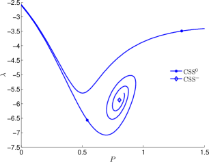
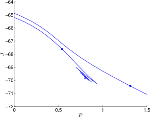
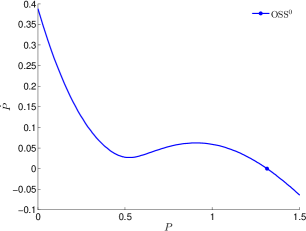
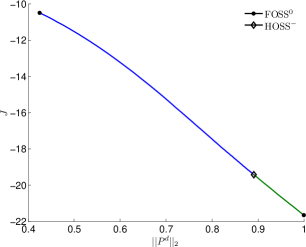
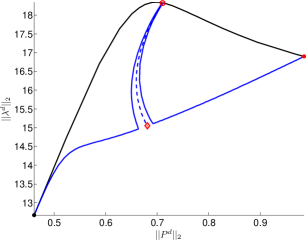
The importance of a numerical analysis of the stable paths comes specifically clear in scenario I with b=0.75𝑏0.75b=0.75. In Fig. 2 we see that there exist three equilibria in the canonical system (two saddles and one unstable focus), whereas the optimal system only consists of one globally stable equilibrium.

Indifference threshold point

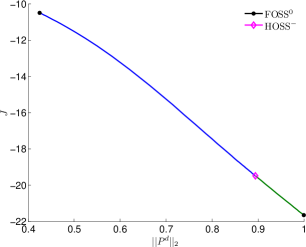
For b=0.65𝑏0.65b=0.65 the number and properties of the equilibria of the canonical system remain the same, but the optimal system consists of two locally stable equilibria separated by an indifference threshold point PIsubscript𝑃𝐼P_{I}, cf. Fig. 3. Thus, a local stability analysis of the equilibria has to be supported by the global analysis the according stable manifolds. Even if the first task can be realized analytically, the stable paths can only be calculated analytically in very rare cases. Usually and specifically in our case we have to resort to numerical methods to solve the latter task.

Indifference point

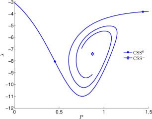
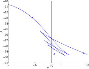
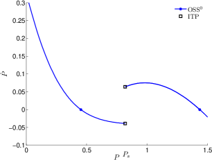
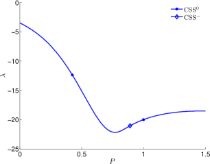
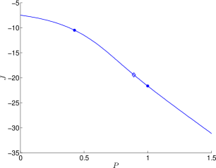
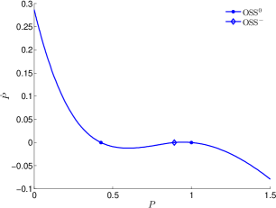
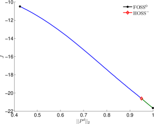
For scenario II with c=3.5𝑐3.5c=3.5 the canonical system exhibits two saddles and one unstable node (cf. Fig. 4a). Calculating the stable paths and comparing the objective values we find that the unstable equilibrium is a threshold point (cf. Fig. 4b). This unstable equilibrium separates the regions of attraction for the two locally stable equilibria corresponding to the two saddles(cf. Fig. 4c). The second case with c=3.0825𝑐3.0825c=3.0825 yields qualitatively the same result and is not depicted.

Refer to caption
(a) Equilibria bifurcation diagram
Refer to caption
(b) Equilibria bifurcation diagram
Figure 1: The \bullet denote equilibria satisfying the SPP and \diamond denote equilibria not satisfying SPP. The figures in the first row show the bifurcation parameter versus the (absolute) state value. In the second row the norm of the equilibrium is plotted versus the bifurcation parameter. Panel LABEL:sub@fig:sl0D_bifan1 (ρ=0.03,c=0.5formulae-sequence𝜌0.03𝑐0.5\rho=0.03,c=0.5 and varying b𝑏b) show the existence of two separated branches of equilibria. In the interval [0,0.727]00.727[0,0.727] there exist three equilibria. Panel LABEL:sub@fig:sl0D_bifan2 (ρ=0.3,b=0.55formulae-sequence𝜌0.3𝑏0.55\rho=0.3,b=0.55 and varying c𝑐c) shows the existence of one branch of equilibria. In the interval [2.566,3.556]2.5663.556[2.566,3.556] there exist three equilibria.
Refer to caption
(a) State-Costate
Refer to caption
(b) State-Objectivevalue
Refer to caption
(c) Optimal System
Figure 2: For ρ=0.03,c=0.5formulae-sequence𝜌0.03𝑐0.5\rho=0.03,\ c=0.5 and b=0.75𝑏0.75b=0.75 there exist three equilibria in the canonical system LABEL:sub@fig:sl_multipleequa. The optimal system LABEL:sub@fig:sl_multipleequc only consist of one globally optimal equilibrium. In panel LABEL:sub@fig:sl_multipleequa the \bullet denote saddles of the canonical system, the \diamond an unstable focus. In panel LABEL:sub@fig:sl_multipleequc the \bullet denotes the globally stable equilibrium.
Refer to caption
(a) State-Costate
Refer to caption
(b) State-Objectivevalue
Refer to caption
(c) Optimal System
Figure 3: For ρ=0.03,c=0.5formulae-sequence𝜌0.03𝑐0.5\rho=0.03,\ c=0.5 and b=0.65𝑏0.65b=0.65 there exist three equilibria in the canonical system LABEL:sub@fig:sl_optmultipleequa. The optimal system LABEL:sub@fig:sl_optmultipleequc consists of two locally optimal equilibria. The basins of attraction are separated by an indifference threshold point (Skiba point) PIsubscript𝑃𝐼P_{I}, with a discontinuous dynamics at PIsubscript𝑃𝐼P_{I}. In panel LABEL:sub@fig:sl_optmultipleequa the \bullet denote saddles of the canonical system, the \diamond an unstable focus. In panel LABEL:sub@fig:sl_optmultipleequc the \bullet denote the locally stable equilibria.
Refer to caption
(a) State-Costate
Refer to caption
(b) State-Objectivevalue
Refer to caption
(c) Optimal System
Figure 4: For ρ=0.3,c=3.5formulae-sequence𝜌0.3𝑐3.5\rho=0.3,\ c=3.5 and b=0.55𝑏0.55b=0.55 there exist three equilibria in the canonical system LABEL:sub@fig:sl_optmultipleequa. The optimal system LABEL:sub@fig:sl_optmultipleequc consists of two locally optimal equilibria. The basins of attraction are separated by the optimal unstable equilibrium P^usubscript^𝑃𝑢\hat{P}_{u}. In panel LABEL:sub@fig:sl_optmultipleuniqueequa \bullet denote saddles of the canonical system, \diamond an unstable node. In panel LABEL:sub@fig:sl_optmultipleuniqueequc \bullet denote the locally stable optimal equilibria and \diamond denotes the optimal unstable node.

4 The shallow lake model with spatial diffusion

An extension of the shallow lake model 16 to the class of spatially distributed models, proposed in Brock and Xepapadeas (2008), is given by

maxu(,)0eρtΩln(u(x,t))cP(x,t)dxdtsubscript𝑢superscriptsubscript0superscripte𝜌𝑡subscriptΩ𝑢𝑥𝑡𝑐𝑃𝑥𝑡d𝑥d𝑡\displaystyle\max_{u(\cdot,\cdot)}\int_{0}^{\infty}\operatorname{e}^{-\rho t}\int_{\Omega}\ln(u(x,t))-cP(x,t)\!\operatorname{d}\!x\operatorname{d}\!t (19a)
s.t.tP(x,t)=u(x,t)bP(x,t)+P(x,t)21+P(x,t)2+D2x2P(x,t)s.t.𝑡𝑃𝑥𝑡𝑢𝑥𝑡𝑏𝑃𝑥𝑡𝑃superscript𝑥𝑡21𝑃superscript𝑥𝑡2𝐷superscript2superscript𝑥2𝑃𝑥𝑡\displaystyle\text{s.t.}\quad\frac{\partial}{\partial t}P(x,t)=u(x,t)-bP(x,t)+\frac{P(x,t)^{2}}{1+P(x,t)^{2}}+D\frac{\partial^{2}}{\partial x^{2}}P(x,t) (19b)
nP(x,t)|Ω=0\displaystyle\quad\left.\partial_{n}P(x,t)\right\rvert_{\partial\Omega}=0 (19c)
P(x,t)|t=0=P0(x),xΩ=[L,L].\displaystyle\quad\left.P(x,t)\right\rvert_{t=0}=P_{0}(x),\quad x\in\Omega=[-L,L]\subset\mathbb{R}. (19d)

Contrary to Brock and Xepapadeas (2008) we formulated the problem for Neumann conditions Eq. 19c, the so called zero flux boundary condition, instead of the periodic boundary conditions. From an interpretational point of view we assume the lakes to be located consecutively in a row and there is no flow out of lake. Periodic boundary conditions refer to a ring of lakes. Brock and Xepapadeas argue that they use periodic boundary conditions to exclude effects induced by the conditions at the end points. Anyhow, since this point does not touch our argument that it is necessary to analyze the global behavior of the optimally controlled system, we changed the model formulation in this respect.

Using the (FDM) discretization proposed in Section 2.2 we find

maxu0(),,uN(){0ertG(P0(t),,PN(t),u0(t),,uN(t))dt}subscriptsubscript𝑢0subscript𝑢𝑁superscriptsubscript0superscripte𝑟𝑡𝐺subscript𝑃0𝑡subscript𝑃𝑁𝑡subscript𝑢0𝑡subscript𝑢𝑁𝑡d𝑡\displaystyle\max_{u_{0}(\cdot),\ldots,u_{N}(\cdot)}\left\{\int_{0}^{\infty}\operatorname{e}^{-rt}G(P_{0}(t),\ldots,P_{N}(t),u_{0}(t),\ldots,u_{N}(t))\,\operatorname{d}\!t\right\} (20a)
s.t. P˙i(t)=ui(t)bPi(t)+Pi(t)21+Pi(t)2+D~(Pi1(t)2Pi(t)+Pi+1(t))subscript˙𝑃𝑖𝑡subscript𝑢𝑖𝑡𝑏subscript𝑃𝑖𝑡subscript𝑃𝑖superscript𝑡21subscript𝑃𝑖superscript𝑡2~𝐷subscript𝑃𝑖1𝑡2subscript𝑃𝑖𝑡subscript𝑃𝑖1𝑡\displaystyle\dot{P}_{i}(t)=u_{i}(t)-bP_{i}(t)+\frac{P_{i}(t)^{2}}{1+P_{i}(t)^{2}}+\tilde{D}\left(P_{i-1}(t)-2P_{i}(t)+P_{i+1}(t)\right) (20b)
P1(t)P1(t)=PN+1(t)PN1(t)=0,t0formulae-sequencesubscript𝑃1𝑡subscript𝑃1𝑡subscript𝑃𝑁1𝑡subscript𝑃𝑁1𝑡0𝑡0\displaystyle P_{1}(t)-P_{-1}(t)=P_{N+1}(t)-P_{N-1}(t)=0,\quad t\geq 0 (20c)
Pi(0)=Pi,0>0subscript𝑃𝑖0subscript𝑃𝑖00\displaystyle P_{i}(0)=P_{i,0}>0 (20d)
with
xi=iN,i=0,,N,D~:=D(N2L)2formulae-sequencesubscript𝑥𝑖𝑖𝑁formulae-sequence𝑖0𝑁assign~𝐷𝐷superscript𝑁2𝐿2\displaystyle x_{i}=\frac{i}{N},\quad i=0,\ldots,N,\quad\tilde{D}:=D\left(\frac{N}{2L}\right)^{2}
Pi(t):=P(xi,t),ui(t):=u(xi,t)formulae-sequenceassignsubscript𝑃𝑖𝑡𝑃subscript𝑥𝑖𝑡assignsubscript𝑢𝑖𝑡𝑢subscript𝑥𝑖𝑡\displaystyle P_{i}(t):=P(x_{i},t),\quad u_{i}(t):=u(x_{i},t)
Pi:=P(xi,),ui:=u(xi,)formulae-sequenceassignsubscript𝑃𝑖𝑃subscript𝑥𝑖assignsubscript𝑢𝑖𝑢subscript𝑥𝑖\displaystyle P_{i}:=P(x_{i},\cdot),\quad u_{i}:=u(x_{i},\cdot)
G(P0,,PN,u0,,uN):=1Ni=1N1g(Pi,ui)+g(P0,u0)+g(PN,uN)2assign𝐺subscript𝑃0subscript𝑃𝑁subscript𝑢0subscript𝑢𝑁1𝑁superscriptsubscript𝑖1𝑁1𝑔subscript𝑃𝑖subscript𝑢𝑖𝑔subscript𝑃0subscript𝑢0𝑔subscript𝑃𝑁subscript𝑢𝑁2\displaystyle G(P_{0},\ldots,P_{N},u_{0},\ldots,u_{N}):=\frac{1}{N}\sum_{i=1}^{N-1}g(P_{i},u_{i})+\frac{g(P_{0},u_{0})+g(P_{N},u_{N})}{2}
g(Pi,ui):=ln(ui)cPi2assign𝑔subscript𝑃𝑖subscript𝑢𝑖subscript𝑢𝑖𝑐superscriptsubscript𝑃𝑖2\displaystyle g(P_{i},u_{i}):=\ln(u_{i})-cP_{i}^{2}

Applying Pontryagin’s Maximum Principle on Eqs. 11 yields the canonical system

P˙i(t)=ui(t)bPi(t)+Pi(t)21+Pi(t)2+𝒟i(P)(t)subscript˙𝑃𝑖𝑡subscriptsuperscript𝑢𝑖𝑡𝑏subscript𝑃𝑖𝑡subscript𝑃𝑖superscript𝑡21subscript𝑃𝑖superscript𝑡2subscriptsuperscript𝒟𝑃𝑖𝑡\displaystyle\dot{P}_{i}(t)=u^{\circ}_{i}(t)-bP_{i}(t)+\frac{P_{i}(t)^{2}}{1+P_{i}(t)^{2}}+{\cal D}^{(P)}_{i}(t) (21a)
λ˙i(t)=ciPi(t)+λi(t)(ρ+b2Pi(t)(1+Pi(t)2)2)𝒟i(λ)(t)subscript˙𝜆𝑖𝑡subscript𝑐𝑖subscript𝑃𝑖𝑡subscript𝜆𝑖𝑡𝜌𝑏2subscript𝑃𝑖𝑡superscript1subscript𝑃𝑖superscript𝑡22subscriptsuperscript𝒟𝜆𝑖𝑡\displaystyle\dot{\lambda}_{i}(t)=c_{i}P_{i}(t)+\lambda_{i}(t)\left(\rho+b-\frac{2P_{i}(t)}{\left(1+P_{i}(t)^{2}\right)^{2}}\right)-{\cal D}^{(\lambda)}_{i}(t) (21b)
Pi(0)=Pi,0>0,i=0,,Nformulae-sequencesubscript𝑃𝑖0subscript𝑃𝑖00𝑖0𝑁\displaystyle P_{i}(0)=P_{i,0}>0,\quad i=0,\ldots,N (21c)
ui(t)={12λi(t)i=0,N1λi(t)i=1,,N1superscriptsubscript𝑢𝑖𝑡cases12subscript𝜆𝑖𝑡𝑖0𝑁1subscript𝜆𝑖𝑡𝑖1𝑁1\displaystyle u_{i}^{\circ}(t)=\begin{cases}-\dfrac{1}{2\lambda_{i}(t)}&i=0,N\\ -\dfrac{1}{\lambda_{i}(t)}&i=1,\ldots,N-1\end{cases} (21d)
ci:={ci=0,N2ci=1,,N1assignsubscript𝑐𝑖cases𝑐𝑖0𝑁2𝑐𝑖1𝑁1\displaystyle c_{i}:=\begin{cases}c&i=0,N\\ 2c&i=1,\ldots,N-1\end{cases}
𝒟i(P)(t):={2D~(P1(t)P0(t))i=0D~(Pi1(t)2Pi(t)+Pi+1(t))i=1,,N12D~(PN1(t)PN(t))i=Nassignsubscriptsuperscript𝒟𝑃𝑖𝑡cases2~𝐷subscript𝑃1𝑡subscript𝑃0𝑡𝑖0~𝐷subscript𝑃𝑖1𝑡2subscript𝑃𝑖𝑡subscript𝑃𝑖1𝑡𝑖1𝑁12~𝐷subscript𝑃𝑁1𝑡subscript𝑃𝑁𝑡𝑖𝑁\displaystyle{\cal D}^{(P)}_{i}(t):=\begin{cases}2\tilde{D}(P_{1}(t)-P_{0}(t))&i=0\\ \tilde{D}(P_{i-1}(t)-2P_{i}(t)+P_{i+1}(t))&i=1,\ldots,N-1\\ 2\tilde{D}(P_{N-1}(t)-P_{N}(t))&i=N\end{cases}
𝒟i(λ)(t):={D~(λ1(t)2λ0(t))i=0D~(2λ0(t)2λ1(t)+λ2(t))i=1D~(λi1(t)2λi(t)+λi+1(t))i=2,,N2D~(λN2(t)2λN1(t)+2λN(t))i=N1D~(λN1(t)2λN(t))i=Nassignsubscriptsuperscript𝒟𝜆𝑖𝑡cases~𝐷subscript𝜆1𝑡2subscript𝜆0𝑡𝑖0~𝐷2subscript𝜆0𝑡2subscript𝜆1𝑡subscript𝜆2𝑡𝑖1~𝐷subscript𝜆𝑖1𝑡2subscript𝜆𝑖𝑡subscript𝜆𝑖1𝑡𝑖2𝑁2~𝐷subscript𝜆𝑁2𝑡2subscript𝜆𝑁1𝑡2subscript𝜆𝑁𝑡𝑖𝑁1~𝐷subscript𝜆𝑁1𝑡2subscript𝜆𝑁𝑡𝑖𝑁\displaystyle{\cal D}^{(\lambda)}_{i}(t):=\begin{cases}\tilde{D}(\lambda_{1}(t)-2\lambda_{0}(t))&i=0\\ \tilde{D}(2\lambda_{0}(t)-2\lambda_{1}(t)+\lambda_{2}(t))&i=1\\ \tilde{D}(\lambda_{i-1}(t)-2\lambda_{i}(t)+\lambda_{i+1}(t))&i=2,\ldots,N-2\\ \tilde{D}(\lambda_{N-2}(t)-2\lambda_{N-1}(t)+2\lambda_{N}(t))&i=N-1\\ \tilde{D}(\lambda_{N-1}(t)-2\lambda_{N}(t))&i=N\end{cases}

In Appendix B the details for an implementation of the model 20 in OCMat are explained.

4.1 Equilibria of the canonical/optimal system

There is an intimate relation between the CSS of the canonical system Eq. 17 and FCSS of the canonical system Eq. 21

Corollary 4.1.

Let (P^d,u^d)2N+2superscript^𝑃𝑑superscript^𝑢𝑑superscript2𝑁2(\hat{P}^{d},\hat{u}^{d})\in\mathbb{R}^{2N+2} be FOSS then (P^0d,1/(2u0))subscriptsuperscript^𝑃𝑑012subscript𝑢0(\hat{P}^{d}_{0},1/(2u_{0})) is an equilibrium of the canonical system Eq. 17.

Corollary 4.2.

Let (P^,λ^)^𝑃^𝜆(\hat{P},\hat{\lambda}) be an equilibrium of the canonical system Eq. 17. Then P^d:=(P^,,P^)assignsuperscript^𝑃𝑑^𝑃^𝑃\hat{P}^{d}:=(\hat{P},\ldots,\hat{P}) and λ^d:=(2λ^,λ^,,λ^,2λ^)assignsuperscript^𝜆𝑑2^𝜆^𝜆^𝜆2^𝜆\hat{\lambda}^{d}:=(2\hat{\lambda},\hat{\lambda},\ldots,\hat{\lambda},2\hat{\lambda}) is a FCSS.

Corollary 4.3.

Let (P^,λ^)^𝑃^𝜆(\hat{P},\hat{\lambda}) be a saddle of the canonical system Eq. 17. Then for D~~𝐷\tilde{D} small enough (P^d,λ^d)2N+2superscript^𝑃𝑑superscript^𝜆𝑑superscript2𝑁2(\hat{P}^{d},\hat{\lambda}^{d})\in\mathbb{R}^{2N+2} defined in Corollary 4.2 is FCSS0.

PCSS can in general not be calculated analytically therefore we have to resort to numerical methods. Using Corollary 4.2 we can start a bifurcation analysis of Eq. 21 with an equilibrium of Eq. 17. The PCSS emerge from branching points of the bifurcation curve. In Grass and Uecker (2015) the according bifurcation analysis is done using pde2path, a MATLAB package for the bifurcation analysis of elliptic PDEs, see Uecker et al. (2014) and Dohnal et al. (2014). Since the actual model 16 is a 0D optimal control model with a finite number of states (N+1𝑁1N+1) the bifurcation analysis of Eq. 21 is done using a modified version of CL_MATCONT222This modified version is available from the author..

We analyzed the two different scenarios specified in Table 1.

First Scenario

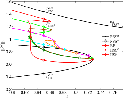
The according bifurcation analysis with respect to b𝑏b is depicted in Fig. 5a. The black curves represent the bifurcation curves of the FCSS. These curves exhibit the same shape as the corresponding bifurcation curves for the 0D model in Fig. 1a. For the lower branch we additionally find four branching points \circ, where the branches of the PCSS emanate (red, green, magenta and cyan). Along the bifurcation curves of the PCSS we find additional branching points and calculated the according bifurcation curves (brown, dark green and orange). Thus, for b=0.65𝑏0.65b=0.65 we find in total two FCSS0 (correspondig to the oligotrophic and eutrophic equilibrium in the 0D model), one FCSS-, thirteen PCSS- and one PCSS0. In fact the brown and dark green branch consists of two distinct bifurcation curves with equilibria that are spatially symmetric.

Second Scenario

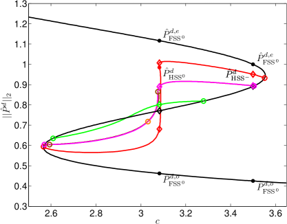
The according bifurcation analysis with respect to c𝑐c is depicted in Fig. 5b. The black bifurcation curve of the FCSS consists of one branch, exhibiting two fold bifurcations and six branching points \circ. These six branching points are connected by three bifurcation curves of the PCSS (red, magenta and green). The red and green curve consist of two spatially symmetric branches. From the magenta PCSS bifurcation curve two further PCSS branches emanate (brown and orange).

In Section 4.4 we consider two specific cases for c=3.5𝑐3.5c=3.5 and c=3.0825𝑐3.0825c=3.0825. In the first case there exist two FCSS0 (correspondig to the oligotrophic and eutrophic equilibrium in the 0D model), one FCSS-, ten PCSS- and two PCSS0. In the latter case there exist two FCSS0, one FCSS- and four PCSS-.
Refer to caption
(a) First Scenario b𝑏b, ρ=0.03,c=0.5formulae-sequence𝜌0.03𝑐0.5\rho=0.03,c=0.5
Refer to caption
(b) Second Scenario c𝑐c, ρ=0.3,b=0.55formulae-sequence𝜌0.3𝑏0.55\rho=0.3,b=0.55
Figure 5: A bifurcation analysis for the canonical system Eq. 21 is depicted in LABEL:sub@fig:sld_bifdiag1 and LABEL:sub@fig:sld_bifdiag2. The symbols: \bullet denote equilibria satisfying the SPP, \diamond equilibria not satisfying the SPP and \circ branching points of the equilibria manifold. The FOSS curves are black and the HOSS curves are colored. Along the red HOSS curve two fold bifurcations occur, the HOSS candidates between these fold bifurcations satisfy the SPP.

4.2 First scenario optimal solutions exemplified on two cases

Most of the results for the specific cases b=0.75𝑏0.75b=0.75 and b=0.65𝑏0.65b=0.65 have already been discussed in Grass and Uecker (2015). Therefore we only give a brief summary and concentrate on some aspects that were easier to get using OCMat.

For b=0.75𝑏0.75b=0.75 there exists a single FOSS, structurally reproducing the result of the according 0D model.

For b=0.65𝑏0.65b=0.65 the main results are

  • None of the PCSS are optimal.

  • The two FCSS0 are optimal.

  • The according basins of attractions are separated by an indifference threshold manifold.

  • In Grass and Uecker (2015) we computed a homogeneous and patterned indifference threshold point. The homogeneous indifference threshold point coincides with the value of the indifference threshold point in model 16.

Next we explain in detail the calculation of a solution converging to an equilibrium satisfying SPP. Subsequently the necessary steps for the detection of an indifference threshold point are explained. Details for the calculation in OCMat can be found in Appendix B.

4.3 A locally optimal patterned equilibrium

To prove that PCSS0 (P^PCSS0d,λ^PCSS0d)subscriptsuperscript^𝑃𝑑PCSS0subscriptsuperscript^𝜆𝑑PCSS0(\hat{P}^{d}_{\text{{PCSS}${}^{0}$}},\hat{\lambda}^{d}_{\text{{PCSS}${}^{0}$}}), see Fig. 5a, is an optimal equilibrium we have to show that there exist no other solution (Pd(),ud())superscript𝑃𝑑superscript𝑢𝑑(P^{d}(\cdot),u^{d}(\cdot)) with Pd(0)=P^PCSS0dsuperscript𝑃𝑑0subscriptsuperscript^𝑃𝑑PCSS0P^{d}(0)=\hat{P}^{d}_{\text{{PCSS}${}^{0}$}} yielding a larger objective value. There exist two other equilibria satisfying SPP, namely the two FCSS0, the oligotrophic (P^FCSS0d,o,P^FCSS0d,o)subscriptsuperscript^𝑃𝑑𝑜FCSS0subscriptsuperscript^𝑃𝑑𝑜FCSS0(\hat{P}^{d,o}_{\text{{FCSS}${}^{0}$}},\hat{P}^{d,o}_{\text{{FCSS}${}^{0}$}}) and the eutrophic FCSS0 (P^FCSS0d,e,λ^FCSS0d,e)subscriptsuperscript^𝑃𝑑𝑒FCSS0subscriptsuperscript^𝜆𝑑𝑒FCSS0(\hat{P}^{d,e}_{\text{{FCSS}${}^{0}$}},\hat{\lambda}^{d,e}_{\text{{FCSS}${}^{0}$}}) (cf. Fig. 5a). For each of these equilibria there may exist a path with Pd(0)=P^PCSS0dsuperscript𝑃𝑑0subscriptsuperscript^𝑃𝑑PCSS0P^{d}(0)=\hat{P}^{d}_{\text{{PCSS}${}^{0}$}} and converging to the oligotrophic/eutrophic equilibrium. To determine these paths we consider the corresponding homotopy problems Eq. 25 with x1subscript𝑥1x_{1} replaced by P^PCSS0dsubscriptsuperscript^𝑃𝑑PCSS0\hat{P}^{d}_{\text{{PCSS}${}^{0}$}}, starting at the equilibrium (P^FCSS0d,o,P^FCSS0d,o)subscriptsuperscript^𝑃𝑑𝑜FCSS0subscriptsuperscript^𝑃𝑑𝑜FCSS0(\hat{P}^{d,o}_{\text{{FCSS}${}^{0}$}},\hat{P}^{d,o}_{\text{{FCSS}${}^{0}$}}) and (P^FCSS0d,e,λ^FCSS0d,e)subscriptsuperscript^𝑃𝑑𝑒FCSS0subscriptsuperscript^𝜆𝑑𝑒FCSS0(\hat{P}^{d,e}_{\text{{FCSS}${}^{0}$}},\hat{\lambda}^{d,e}_{\text{{FCSS}${}^{0}$}}), respectively.

4.3.1 Comparison with equilibrium solution

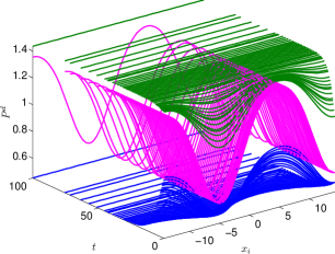
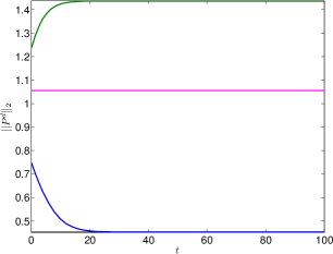
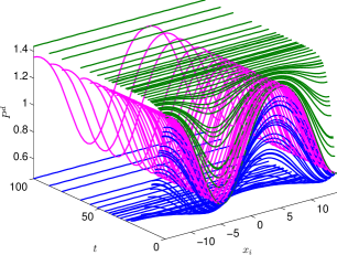
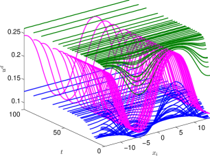
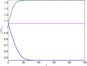
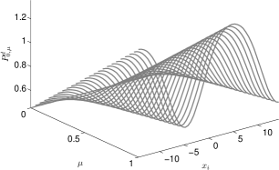
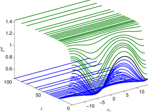
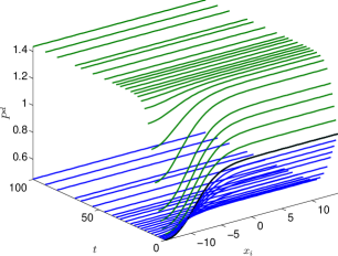
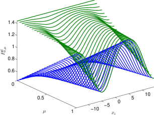
The result of these computations is depicted in Fig. 6. Figure 6a illustrates the “embedding” Eq. 25b. The green manifold proceed from the flat eutrophic states P^FCSS0d,esubscriptsuperscript^𝑃𝑑𝑒FCSS0\hat{P}^{d,e}_{\text{{FCSS}${}^{0}$}} and the blue manifold from the flat oligotrophic states P^FCSS0d,osubscriptsuperscript^𝑃𝑑𝑜FCSS0\hat{P}^{d,o}_{\text{{FCSS}${}^{0}$}} to the patterned states P^PCSS0dsubscriptsuperscript^𝑃𝑑PCSS0\hat{P}^{d}_{\text{{PCSS}${}^{0}$}}. During the continuation of κ𝜅\kappa from zero to one the initial states lie in these manifolds. In Figs. 6b and 6c the states and their norm of the solution paths for κ=0.5𝜅0.5\kappa=0.5 are shown (green and blue). Additionally the states and norm of the equilibrium solution P^PCSS0dsubscriptsuperscript^𝑃𝑑PCSS0\hat{P}^{d}_{\text{{PCSS}${}^{0}$}} are depicted.

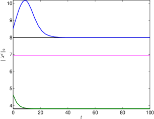
Figures 6d, 6f and 6e display the final results for κ=1𝜅1\kappa=1 also including the figure with the control paths. Moreover, Fig. 6g and Fig. 6e reveal that the values of the costates and hence the controls of the three solutions with Pd(0)=P^PCSS0dsuperscript𝑃𝑑0subscriptsuperscript^𝑃𝑑PCSS0P^{d}(0)=\hat{P}^{d}_{\text{{PCSS}${}^{0}$}} are different.

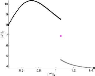
Figure 6h show the slice manifolds (see Definition A.1) in the state-costate space. Each marker ×\times denotes a continuation step.

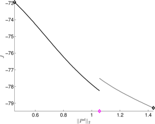
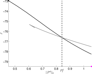
In Fig. 6e the objective values along the slice manifolds are plotted, i.e. the objective values are plotted against the (norm) of the initial points. We see that the final solutions for κ=1𝜅1\kappa=1 both yield a higher objective value and the eutrophic solution converging to FCSS02 dominates the other solutions. On the other hand the gradients of the curves suggest that they eventually intersect. Such an intersection point characterizes an indifference threshold point (cf. Fig. 3b for the 0D model).

4.3.2 Detection and Continuation of an indifference threshold point ITP

To find a possible intersection point of the objective values along the slice manifolds we have to assure that the slice manifolds are comparable and have to check if they intersect (see Definition A.2). The slice manifolds depicted in Fig. 6h are, e.g., not comparable, simply because the manifolds

{P^FCSS0d,o+(1α1)(P^PCSS0dP^FCSS0d,o):α1}conditional-setsubscriptsuperscript^𝑃𝑑𝑜FCSS01subscript𝛼1subscriptsuperscript^𝑃𝑑PCSS0subscriptsuperscript^𝑃𝑑𝑜FCSS0subscript𝛼1\displaystyle\{\hat{P}^{d,o}_{\text{{FCSS}${}^{0}$}}+(1-\alpha_{1})(\hat{P}^{d}_{\text{{PCSS}${}^{0}$}}-\hat{P}^{d,o}_{\text{{FCSS}${}^{0}$}}):\ \alpha_{1}\in\mathbb{R}\}
{P^FCSS0d,e+(1α2)(P^PCSS0dP^FCSS0d,e):α2}.conditional-setsubscriptsuperscript^𝑃𝑑𝑒FCSS01subscript𝛼2subscriptsuperscript^𝑃𝑑PCSS0subscriptsuperscript^𝑃𝑑𝑒FCSS0subscript𝛼2\displaystyle\{\hat{P}^{d,e}_{\text{{FCSS}${}^{0}$}}+(1-\alpha_{2})(\hat{P}^{d}_{\text{{PCSS}${}^{0}$}}-\hat{P}^{d,e}_{\text{{FCSS}${}^{0}$}}):\ \alpha_{2}\in\mathbb{R}\}.

are different. See Fig. 6a), where the green and blue curves depict (parts) of these manifolds. Only if slice manifolds are comparable and have a non-empty intersection this means that the solutions corresponding to the intersection points of the slice manifold start at the same initial states and hence their objective values can be compared.

Anyhow, since the solution starting at P^PCSS0dsubscriptsuperscript^𝑃𝑑PCSS0\hat{P}^{d}_{\text{{PCSS}${}^{0}$}} and converging to FCSS02 is known we can start the homotopy BVP 25 with

X(0)=P^PCSS0d+(1κ)(P^FCSS0d,oP^PCSS0d).𝑋0subscriptsuperscript^𝑃𝑑PCSS01𝜅subscriptsuperscript^𝑃𝑑𝑜FCSS0subscriptsuperscript^𝑃𝑑PCSS0X(0)=\hat{P}^{d}_{\text{{PCSS}${}^{0}$}}+(1-\kappa)(\hat{P}^{d,o}_{\text{{FCSS}${}^{0}$}}-\hat{P}^{d}_{\text{{PCSS}${}^{0}$}}).

In that case the manifolds

{P^FCSS0d,o+(1α1)(P^PCSS0dP^FCSS0d,o):α1}conditional-setsubscriptsuperscript^𝑃𝑑𝑜FCSS01subscript𝛼1subscriptsuperscript^𝑃𝑑PCSS0subscriptsuperscript^𝑃𝑑𝑜FCSS0subscript𝛼1\displaystyle\{\hat{P}^{d,o}_{\text{{FCSS}${}^{0}$}}+(1-\alpha_{1})(\hat{P}^{d}_{\text{{PCSS}${}^{0}$}}-\hat{P}^{d,o}_{\text{{FCSS}${}^{0}$}}):\ \alpha_{1}\in\mathbb{R}\}
{P^PCSS0d+(1κ)(P^FCSS0d,oP^PCSS0d):κ}.conditional-setsubscriptsuperscript^𝑃𝑑PCSS01𝜅subscriptsuperscript^𝑃𝑑𝑜FCSS0subscriptsuperscript^𝑃𝑑PCSS0𝜅\displaystyle\{\hat{P}^{d}_{\text{{PCSS}${}^{0}$}}+(1-\kappa)(\hat{P}^{d,o}_{\text{{FCSS}${}^{0}$}}-\hat{P}^{d}_{\text{{PCSS}${}^{0}$}}):\ \kappa\in\mathbb{R}\}.

trivially coincide and the slice manifolds are comparable, see Fig. 7a. Moreover the slice manifolds intersect and and the corresponding objective values curves intersect at an indifference threshold point PI,1dsubscriptsuperscript𝑃𝑑𝐼1P^{d}_{I,1} (cf. Fig. 7d).

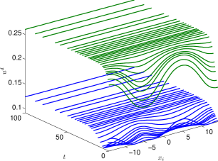
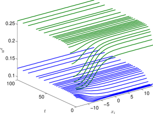
In Fig. 7b and Fig. 7e the corresponding state Pe,od()superscriptsubscript𝑃𝑒𝑜𝑑P_{e,o}^{d}(\cdot) and control paths ue,od())u_{e,o}^{d}(\cdot)) are shown.

Repeating the same procedure for the three two FCSS0 and PCSS0 we find that PCSS0 is not optimal and again we find a further indifference threshold point PI,2dsubscriptsuperscript𝑃𝑑𝐼2P^{d}_{I,2}. The according solutions are depicted in Fig. 7c and Fig. 7f.

It is an interesting question to see how we can find indifference threshold points “between” PI,1dsubscriptsuperscript𝑃𝑑𝐼1P^{d}_{I,1} and PI,2dsubscriptsuperscript𝑃𝑑𝐼2P^{d}_{I,2}. Let us recall that we found the indifference threshold points by the intersection of two n𝑛n dimensional manifolds (with n=N+1𝑛𝑁1n=N+1 the number of states Pdsuperscript𝑃𝑑P^{d}) in the n+1𝑛1n+1 dimensional space (Pd,J(Pd(0)))superscript𝑃𝑑𝐽superscript𝑃𝑑0(P^{d},J(P^{d}(0))). Generically this yields an n1=N𝑛1𝑁n-1=N dimensional manifold. Already for the discretization N=50𝑁50N=50 its dimension is too large to recover the entire indifference threshold manifold (in the original PDE problem the dimension actually increases to infinity). Anyhow, we can e.g. search for indifference threshold points along the linear connection PI,2d+(1κ)(PI,1dPI,2d)subscriptsuperscript𝑃𝑑𝐼21𝜅subscriptsuperscript𝑃𝑑𝐼1subscriptsuperscript𝑃𝑑𝐼2P^{d}_{I,2}+(1-\kappa)(P^{d}_{I,1}-P^{d}_{I,2}). The result is depicted in an animation embedded into Fig. 7e. The according BVP for the numerical solution of this problem is presented in Section A.2.2.
Refer to caption
(a) Manifolds of initial distributions
Refer to caption
(b) State paths at κ=0.5𝜅0.5\kappa=0.5
Refer to caption
(c) Norm of the states at κ=0.5𝜅0.5\kappa=0.5
Refer to caption
(d) State paths at κ=1𝜅1\kappa=1
Refer to caption
(e) Control paths at κ=1𝜅1\kappa=1
Refer to caption
(f) Norm of the states at κ=1𝜅1\kappa=1
Refer to caption
(g) Norm of the costates at κ=1𝜅1\kappa=1
Refer to caption
(h) Slice manifolds
Refer to caption
(i) Objective values at slice manifolds
Figure 6: This figure presents the steps of the continuation process to find solutions starting at Pd(0)=P^PCSS0dsuperscript𝑃𝑑0subscriptsuperscript^𝑃𝑑PCSS0P^{d}(0)=\hat{P}^{d}_{\text{{PCSS}${}^{0}$}} and converging to the oligotrophic and eutrophic FCSS0. The colors refer to the eutrophic (blue), oligotrophic (green) and patterned (magenta) solutions. In LABEL:sub@fig:foss2hossb051 the manifolds of initial distributions, that are passed through the continuation, are depicted. For the continuation parameter κ=0.5𝜅0.5\kappa=0.5 the state paths and corresponding norms are shown in LABEL:sub@fig:foss2hossb052 and LABEL:sub@fig:foss2hossb053. The final results are illustrated in LABEL:sub@fig:foss2hossb054 (state paths), LABEL:sub@fig:foss2hossb057 (control paths), LABEL:sub@fig:foss2hossb055 (costate paths), and LABEL:sub@fig:foss2hossb056 (norms). In LABEL:sub@fig:foss2hossb058 the corresponding slice manifolds are shown in the state-costate space. The objective values for solutions of the slice manifolds in LABEL:sub@fig:foss2hossb059 show that the path converging to the oligotrophic equilibrium is optimal among all solutions that start in Pd(0)=P^PCSS0dsuperscript𝑃𝑑0subscriptsuperscript^𝑃𝑑PCSS0P^{d}(0)=\hat{P}^{d}_{\text{{PCSS}${}^{0}$}}.


Refer to caption
(a) Manifold of initial distributions
Refer to caption
(b) State paths of Skiba solution
Refer to caption
(c) State paths of Skiba solution
Refer to caption
(d) Crossing of objective values
Refer to caption
(e) Control paths of Skiba solution
Refer to caption
(f) Control paths of Skiba solution
Figure 7: This figure shows the detection of a patterned Skiba distribution and its continuation to a different Skiba distribution on the Skiba manifold. To receive the animation files associated to the panels LABEL:sub@fig:fossskiba1, LABEL:sub@fig:fossskiba2 and LABEL:sub@fig:fossskiba5 please contact the author.

4.4 Second scenario

In the first scenario with b=0.65𝑏0.65b=0.65 we only found the eutrophic and oligotrophic equilibria being FOSS. This is somehow analogous to the 0D model, where the CSS does not appear in the optimal system (see Fig. 3).

The result for the 0D model in the second scenario shows that beside the eutrophic and oligotrophic CSS0 the unstable node (CSS-) appears as limit of the regions of attractions for the two CSS0. Thus, we can expect that FCSS- is optimal in model 20. Therefore, also PCSS- cannot be excluded to be optimal.

We therefore analyze two different cases with c=3.5𝑐3.5c=3.5 where none of the PCSS satisfy SPP and c=3.0825𝑐3.0825c=3.0825, for which one of the PCSS satisfies SPP. For the original shallow lake model 16 these two cases are qualitatively the same (cf. Fig. 4).

4.4.1 Patterned equilibrium not satisfying SPP

For c=3.5𝑐3.5c=3.5 we try to find solutions that start at the states of the FCSS- (P^FCSS-dsubscriptsuperscript^𝑃𝑑FCSS-\hat{P}^{d}_{\text{{FCSS}${}^{-}$}}) and one of the PCSS- and converge to the eutrophic (oligotrophic) FCSS.

In Fig. 8 the main results of this analysis are depicted. The example depicted in the first column (LABEL:sub@fig:foss2unstI1,LABEL:sub@fig:foss2unstI4 and LABEL:sub@fig:foss2unstI7) is analogous to the case in the 0D model shown in Fig. 4. Thus, it is not possible to find a solution starting at the initial states of the FCSS- and converging to the eutrophic or oligotrophic FCSS. Instead, during the continuation process the initial states of P^FCSS-dsubscriptsuperscript^𝑃𝑑FCSS-\hat{P}^{d}_{\text{{FCSS}${}^{-}$}} are approached but cannot be reached. In Fig. 8a the phase portrait of the final result is plotted, which is analogous to the state-costate space in 0D (cf. Fig. 4a). In Fig. 8c we see that the objective value for the homogeneous initial distributions is continuous (cf. Fig. 4b). Consequently, for spatially homogeneous initial distributions, the optimal path is unique, where P^FCSS-dsubscriptsuperscript^𝑃𝑑FCSS-\hat{P}^{d}_{\text{{FCSS}${}^{-}$}} separates the regions of attractions for the eutrophic (oligotrophic) equilibrium P^FCSS0d,esubscriptsuperscript^𝑃𝑑𝑒FCSS0\hat{P}^{d,e}_{\text{{FCSS}${}^{0}$}} (P^FCSS0d,osubscriptsuperscript^𝑃𝑑𝑜FCSS0\hat{P}^{d,o}_{\text{{FCSS}${}^{0}$}}). The optimal state paths for solutions starting exactly at P^FCSS-dsubscriptsuperscript^𝑃𝑑FCSS-\hat{P}^{d}_{\text{{FCSS}${}^{-}$}} (the equilibrium solution, black) and in the near vicinity (blue and green) are depicted in Fig. 8d. Repeating these steps for each of the PCSS, two examples are depicted in the last two columns of Fig. 8, yields that each of these equilibria is optimal, i.e. are POSS. Since none of the PCSS satisfy SPP these equilibria and their stable manifolds separate the regions of attractions of the FOSS.

At this point a few questions remain unsettled.

  • Is the defect of an equilibrium not satisfying SPP constant for state discretizations that are fine enough?

  • What does this mean for the original PDE problem?

  • Can we say that equilibria not satisfying SPP and their stable manifolds separate the regions of attractions for the solutions satisfying SPP?

  • What is the state space of the PDE problem?

4.4.2 Patterned equilibrium satisfying SPP

In this section we numerically check, whether the unique patterned equilibrium PCSS0 for c=3.0825𝑐3.0825c=3.0825 is POSS(cf. Fig. 5b). For that reason we have to show that there exists no other solution path of the canonical system Eq. 21 that starts at P^PCSS0dsubscriptsuperscript^𝑃𝑑PCSS0\hat{P}^{d}_{\text{{PCSS}${}^{0}$}} yielding a larger objective value. The only other candidates are stable paths of the eutrophic and oligotrophic FCSS0. The result of the numerical comparison for the oligotrohic versus the patterned equilibrium is depicted in Fig. 9d and Fig. 9e.

To find a feasible path (P1d(,κ),λ1d(,κ))superscriptsubscript𝑃1𝑑𝜅superscriptsubscript𝜆1𝑑𝜅(P_{1}^{d}(\cdot,\kappa),\lambda_{1}^{d}(\cdot,\kappa)) that satisfies Pd(0,1)=P^PCSS0dsuperscript𝑃𝑑01subscriptsuperscript^𝑃𝑑PCSS0P^{d}(0,1)=\hat{P}^{d}_{\text{{PCSS}${}^{0}$}} and

limt(P1d(t,κ),λ1d(t,κ))=(P^FCSS0d,o,P^FCSS0d,o)withκ[0,1]formulae-sequencesubscript𝑡superscriptsubscript𝑃1𝑑𝑡𝜅superscriptsubscript𝜆1𝑑𝑡𝜅subscriptsuperscript^𝑃𝑑𝑜FCSS0subscriptsuperscript^𝑃𝑑𝑜FCSS0with𝜅01\lim_{t\to\infty}(P_{1}^{d}(t,\kappa),\lambda_{1}^{d}(t,\kappa))=(\hat{P}^{d,o}_{\text{{FCSS}${}^{0}$}},\hat{P}^{d,o}_{\text{{FCSS}${}^{0}$}})\quad\text{with}\quad\kappa\in[0,1]

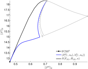
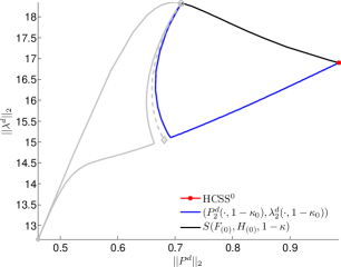
we solve the homotopy problem Eq. 25, starting with the constant equilibrium solution (P^FCSS0d,o,P^FCSS0d,o)subscriptsuperscript^𝑃𝑑𝑜FCSS0subscriptsuperscript^𝑃𝑑𝑜FCSS0(\hat{P}^{d,o}_{\text{{FCSS}${}^{0}$}},\hat{P}^{d,o}_{\text{{FCSS}${}^{0}$}}). The continuation process revealed that it is not possible to find a feasible path for κ=1𝜅1\kappa=1, instead some value κ0<1subscript𝜅01\kappa_{0}<1 was approached. The last computed path (P1d(,κ0),λ1d(,κ0))superscriptsubscript𝑃1𝑑subscript𝜅0superscriptsubscript𝜆1𝑑subscript𝜅0(P_{1}^{d}(\cdot,\kappa_{0}),\lambda_{1}^{d}(\cdot,\kappa_{0})) is shown in Fig. 9a together with the corresponding slice manifold (dashed black).

Next we repeated the procedure for the reversed homotopy problem, starting with the constant patterned solution (P^PCSS0d,λ^PCSS0d)subscriptsuperscript^𝑃𝑑PCSS0subscriptsuperscript^𝜆𝑑PCSS0(\hat{P}^{d}_{\text{{PCSS}${}^{0}$}},\hat{\lambda}^{d}_{\text{{PCSS}${}^{0}$}}) and trying to find a feasible path (P2d(,1κ),λ2d(,1κ))superscriptsubscript𝑃2𝑑1𝜅superscriptsubscript𝜆2𝑑1𝜅(P_{2}^{d}(\cdot,1-\kappa),\lambda_{2}^{d}(\cdot,1-\kappa)) that satisfies Pd(0,0)=P^FCSS0d,osuperscript𝑃𝑑00subscriptsuperscript^𝑃𝑑𝑜FCSS0P^{d}(0,0)=\hat{P}^{d,o}_{\text{{FCSS}${}^{0}$}} and

limt(P2d(t,1κ),λ2d(t,1κ))=(P^PCSS0d,λ^PCSS0d)withκ[0,1].formulae-sequencesubscript𝑡superscriptsubscript𝑃2𝑑𝑡1𝜅superscriptsubscript𝜆2𝑑𝑡1𝜅subscriptsuperscript^𝑃𝑑PCSS0subscriptsuperscript^𝜆𝑑PCSS0with𝜅01\lim_{t\to\infty}(P_{2}^{d}(t,1-\kappa),\lambda_{2}^{d}(t,1-\kappa))=(\hat{P}^{d}_{\text{{PCSS}${}^{0}$}},\hat{\lambda}^{d}_{\text{{PCSS}${}^{0}$}})\quad\text{with}\quad\kappa\in[0,1].

Again the continuation process revealed that it was not possible to find a feasible path for κ=0𝜅0\kappa=0, instead some value approximately 1κ01subscript𝜅01-\kappa_{0} was approached. This solution (P2d(,1κ),λ2d(,1κ))superscriptsubscript𝑃2𝑑1𝜅superscriptsubscript𝜆2𝑑1𝜅(P_{2}^{d}(\cdot,1-\kappa),\lambda_{2}^{d}(\cdot,1-\kappa)) is represented in Fig. 9b by the blue solution path and black slice manifold.

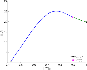
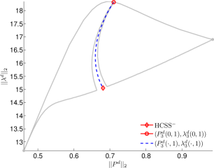
The two last solution paths from both continuation processes suggest that there exists a separating manifold for the regions of attractions of the oligotrophic FCSS0 and PCSS0. A possible candidate for this separating manifold is the stable manifold of the PCSS- with defect 11-1 (see the \diamond in Fig. 9c). To test this conjecture we solved the homotopy problem Eq. 29 for defective equilibria. For x1(1)superscriptsubscript𝑥11x_{1}^{(1)} we took P1d(0,κ0)superscriptsubscript𝑃1𝑑0subscript𝜅0P_{1}^{d}(0,\kappa_{0}) (the initial states of the last continuation step of the first homotopy problem) and set V1:=(1,,1)N+1assignsubscript𝑉111superscript𝑁1V_{1}:=(1,\ldots,1)\in\mathbb{R}^{N+1}, which satisfies the rank condition Eq. 29d. The last solution (P3d(,1),λ3d(,1))superscriptsubscript𝑃3𝑑1superscriptsubscript𝜆3𝑑1(P_{3}^{d}(\cdot,1),\lambda_{3}^{d}(\cdot,1)) of this homotopy problem is depicted as dashed blue curve in Fig. 9d and gives a strong numerical argument for our conjecture.

The overall picture, Fig. 9d, suggests that for every ε>0𝜀0\varepsilon>0 there exists κ1subscript𝜅1\kappa_{1} and κ2subscript𝜅2\kappa_{2} such that there exists solutions (P1d(,κ1),λ1d(,κ1))superscriptsubscript𝑃1𝑑subscript𝜅1superscriptsubscript𝜆1𝑑subscript𝜅1(P_{1}^{d}(\cdot,\kappa_{1}),\lambda_{1}^{d}(\cdot,\kappa_{1})) and (P2d(,1κ2),λ2d(,1κ2))superscriptsubscript𝑃2𝑑1subscript𝜅2superscriptsubscript𝜆2𝑑1subscript𝜅2(P_{2}^{d}(\cdot,1-\kappa_{2}),\lambda_{2}^{d}(\cdot,1-\kappa_{2})) of the homotopy problems with

(P1d(0,κ1),λ1d(0,κ1))(P3d(0,1),λ3d(0,1))2<εsubscriptdelimited-∥∥superscriptsubscript𝑃1𝑑0subscript𝜅1superscriptsubscript𝜆1𝑑0subscript𝜅1superscriptsubscript𝑃3𝑑01superscriptsubscript𝜆3𝑑012𝜀\displaystyle\lVert(P_{1}^{d}(0,\kappa_{1}),\lambda_{1}^{d}(0,\kappa_{1}))-(P_{3}^{d}(0,1),\lambda_{3}^{d}(0,1))\rVert_{2}<\varepsilon
and
(P2d(0,1κ2),λ2d(0,1κ2))(P3d(0,1),λ3d(0,1))2<εsubscriptdelimited-∥∥superscriptsubscript𝑃2𝑑01subscript𝜅2superscriptsubscript𝜆2𝑑01subscript𝜅2superscriptsubscript𝑃3𝑑01superscriptsubscript𝜆3𝑑012𝜀\displaystyle\lVert(P_{2}^{d}(0,1-\kappa_{2}),\lambda_{2}^{d}(0,1-\kappa_{2}))-(P_{3}^{d}(0,1),\lambda_{3}^{d}(0,1))\rVert_{2}<\varepsilon
or even stronger
(P1d(,κ1),λ1d(,κ1))(P3d(,1),λ3d(,1))L2<εsubscriptdelimited-∥∥superscriptsubscript𝑃1𝑑subscript𝜅1superscriptsubscript𝜆1𝑑subscript𝜅1superscriptsubscript𝑃3𝑑1superscriptsubscript𝜆3𝑑1subscript𝐿2𝜀\displaystyle\lVert(P_{1}^{d}(\cdot,\kappa_{1}),\lambda_{1}^{d}(\cdot,\kappa_{1}))-(P_{3}^{d}(\cdot,1),\lambda_{3}^{d}(\cdot,1))\rVert_{L_{2}}<\varepsilon
and
(P2d(,1κ2),λ2d(,1κ2))(P3d(,1),λ3d(,1))L2<ε.subscriptdelimited-∥∥superscriptsubscript𝑃2𝑑1subscript𝜅2superscriptsubscript𝜆2𝑑1subscript𝜅2superscriptsubscript𝑃3𝑑1superscriptsubscript𝜆3𝑑1subscript𝐿2𝜀\displaystyle\lVert(P_{2}^{d}(\cdot,1-\kappa_{2}),\lambda_{2}^{d}(\cdot,1-\kappa_{2}))-(P_{3}^{d}(\cdot,1),\lambda_{3}^{d}(\cdot,1))\rVert_{L_{2}}<\varepsilon.

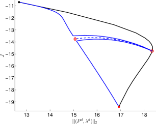
Plotting the objective values evaluated along the solutions of the corresponding slice manifolds shows that the objective function is continuous in the vicinity of P3d(0,1)superscriptsubscript𝑃3𝑑01P_{3}^{d}(0,1), see Fig. 9e. An analogous result holds for the comparison of the stable paths converging to the eutrophic FCSS0 and the PCSS0. This proves the optimality of FCSS0 and PCSS0 as well. Also according to the case c=3.5𝑐3.5c=3.5 the stable manifolds of defective equilibria separate the regions of attractions of the equilibria satisfying SPP.

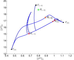
Figure 9f shows (part of) a phase portrait in the state-costate space for c=3.0825𝑐3.0825c=3.0825. The subscripts of the equilibria denote the defect of the according equilibrium. Thus, there exist two FCSS0 (P^FCSS0d,esubscriptsuperscript^𝑃𝑑𝑒FCSS0\hat{P}^{d,e}_{\text{{FCSS}${}^{0}$}} and P^FCSS0d,osubscriptsuperscript^𝑃𝑑𝑜FCSS0\hat{P}^{d,o}_{\text{{FCSS}${}^{0}$}}), and one PCSS0 (P^PCSS0dsubscriptsuperscript^𝑃𝑑PCSS0\hat{P}^{d}_{\text{{PCSS}${}^{0}$}}). Additionally a few paths are plotted that converge to P^FCSS0d,e,P^FCSS0d,osubscriptsuperscript^𝑃𝑑𝑒FCSS0subscriptsuperscript^𝑃𝑑𝑜FCSS0\hat{P}^{d,e}_{\text{{FCSS}${}^{0}$}},\ \hat{P}^{d,o}_{\text{{FCSS}${}^{0}$}}, and P^PCSS0dsubscriptsuperscript^𝑃𝑑PCSS0\hat{P}^{d}_{\text{{PCSS}${}^{0}$}} (solid blue) and to PCSS- with defect 11-1 (dashed blue). The specific case for solutions that converge to the oligotrophic equilibrium (P^FCSS0d,o,P^FCSS0d,o)subscriptsuperscript^𝑃𝑑𝑜FCSS0subscriptsuperscript^𝑃𝑑𝑜FCSS0(\hat{P}^{d,o}_{\text{{FCSS}${}^{0}$}},\hat{P}^{d,o}_{\text{{FCSS}${}^{0}$}}) and patterned equilibrium (P^PCSS0d,λ^PCSS0d)subscriptsuperscript^𝑃𝑑PCSS0subscriptsuperscript^𝜆𝑑PCSS0(\hat{P}^{d}_{\text{{PCSS}${}^{0}$}},\hat{\lambda}^{d}_{\text{{PCSS}${}^{0}$}}) is separately illustrated in Fig. 9d and Fig. 9e.
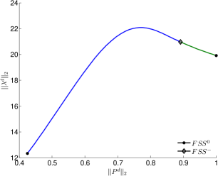
Refer to caption
(a) Continuation to Pd(0)P^FCSS-dsuperscript𝑃𝑑0subscriptsuperscript^𝑃𝑑FCSS-P^{d}(0)\approx\hat{P}^{d}_{\text{{FCSS}${}^{-}$}}
Refer to caption
(b) Continuation to Pd(0)superscript𝑃𝑑0absentP^{d}(0)\approxP^PCSS-dsubscriptsuperscript^𝑃𝑑PCSS-\hat{P}^{d}_{\text{{PCSS}${}^{-}$}}
Refer to caption
(c) Continuation to Pd(0)superscript𝑃𝑑0absentP^{d}(0)\approxP^PCSS-dsubscriptsuperscript^𝑃𝑑PCSS-\hat{P}^{d}_{\text{{PCSS}${}^{-}$}}
Refer to caption
(d) State paths starting near P^FCSS-dsubscriptsuperscript^𝑃𝑑FCSS-\hat{P}^{d}_{\text{{FCSS}${}^{-}$}}
Refer to caption
(e) State paths starting near P^PCSS-dsubscriptsuperscript^𝑃𝑑PCSS-\hat{P}^{d}_{\text{{PCSS}${}^{-}$}}
Refer to caption
(f) State paths starting near P^PCSS-dsubscriptsuperscript^𝑃𝑑PCSS-\hat{P}^{d}_{\text{{PCSS}${}^{-}$}}
Refer to caption
(g) Objective value along slice manifolds
Refer to caption
(h) Objective value along slice manifolds
Refer to caption
(i) Objective value along slice manifolds
Figure 8: This figure depicts the numerical proof for the optimality of FCSS- and PCSS- at c=3.5𝑐3.5c=3.5, i.e., the optimality of the equilibria that do not satisfy SPP, exemplified for three equilibria. In the first row LABEL:sub@fig:foss2unstI1-LABEL:sub@fig:foss2unstI3 the slice manifolds for the according continuation processes are depicted in the normed state-costate space. The second row LABEL:sub@fig:foss2unstI4-LABEL:sub@fig:foss2unstI6 shows the state paths for the solutions starting at and near the FCSS- and PCSS-, respectively. The last row LABEL:sub@fig:foss2unstI7-LABEL:sub@fig:foss2unstI9 illustrates that the objective function is continuous in the vicinity of the constant equilibria solutions for the FCSS- and PCSS-. Therefore the equilibria not satisfying SPP are optimal as well.
Refer to caption
(a) Homotopy FCSS0 to PCSS0
Refer to caption
(b) Homotopy PCSS0 to FCSS0
Refer to caption
(c) Homotopy PCSS- to P1(0,κ0)subscript𝑃10subscript𝜅0P_{1}(0,\kappa_{0})
Refer to caption
(e) Objective value
Refer to caption
(f) Phase portrait
Figure 9: In LABEL:sub@fig:fossnhoss1 some of the solutions paths and equilibria in the state-costate space are depicted. The solutions shown in LABEL:sub@fig:fossnhoss3 and LABEL:sub@fig:fossnhoss2 are the result of the continuation processes, when we tried to find a solution starting at the states of POSS and converging to the oligotrophic FOSS, and vice versa. The continuation process approached a state lying on the stable manifold (dashed blue) of the PCSS- with defect 11-1. Thus, for initial states coinciding with the states of the stable manifold with defect 11-1 it is optimal to converge along the stable manifold to the POSS with defect 11-1. In the vicinity of these initial states it is optimal to converge either to the oligotrophic FOSS or the POSS satisfying SPP. To receive the animation file associated to the panel LABEL:sub@fig:fossnhoss3 please contact the author.

Refer to caption
(d) Slice manifolds and solution paths

5 Conclusion

The purpose of this article is the presentation of a numerical framework, that allows us to numerically experiment with 1D spatially distributed optimal control problems. Numerical experiment is meant in the sense of Heaviside, who claimed mathematics as an experimental science, cf. Heaviside (1893).

We were thus able to find numerical evidence for the occurrence of (indifference) threshold distributions in distributed models. Moreover, this points towards a possible generalization of the saddle point property, which in case of multiple canonical steady states (CSS) is intimately connected to the existence of multiple optimal solutions. Even though this simple FDM could also be applied to spatially 2D models, such an approach would immediately become numerically intractable. Therefore, it is an intermediate step to the method of a finite element discretization, that is presented in Grass and Uecker (2015) and extended in Uecker (2015).

Different directions for further research result from the presented approach. The obvious next step is the previously mentioned application of FEM discretization. This is realized as an add-on toolbox (p2pOC) to the MATLAB package pde2path, which is a numerical tool for continuation and bifurcation in 2D elliptic systems, cf. Uecker et al. (2014).333It can be downloaded for free from http://www.staff.uni-oldenburg.de/hannes.uecker/pde2path.

A main drawback of the actual approach is difficulty to handle (inequality) constraints. For a correct usage of the used BVPsolver the rhs of the dynamics has to at least continuously differentiable. This property is violated, when constraints become active. We solved that problem by considering different arcs of the solution path, where each of the arcs satisfied the differentiability condition. For non-distributed models this is in general a practicable way but hardly to realize for distributed models. Simply because for each transition from one arc to the other the according switching conditions have to be stated. This ansatz quickly becomes intractable for the high dimensional discretized system.

Therefore, we will put effort in the development of a solver based on finite element discretization and conjugate gradient method combined with a continuation step.

Appendix A Numerical method implemented in OCMat

In this section we formulate the basic method for the calculation of paths that converge to an equilibrium of the canonical system.

A.1 The core problem

The core problem that has to be solved is the following. Given an equilibrium (x^,λ^)^𝑥^𝜆(\hat{x},\hat{\lambda}) and an initial distribution x0subscript𝑥0x_{0} we want to find a path (x(),λ())𝑥𝜆(x(\cdot),\lambda(\cdot)) satisfying Eq. 3 together with the boundary conditions

x(0)=x0andlimt(x(t),λ(t))=(x^,λ^).formulae-sequence𝑥0subscript𝑥0andsubscript𝑡𝑥𝑡𝜆𝑡^𝑥^𝜆x(0)=x_{0}\quad\text{and}\quad\lim_{t\to\infty}(x(t),\lambda(t))=(\hat{x},\hat{\lambda}). (22)

The dimension of the according eigenspace

0<dimEs(x^,λ^)=nsn.0dimensionsuperscriptE𝑠^𝑥^𝜆subscript𝑛𝑠𝑛0<\dim\operatorname{E}^{s}(\hat{x},\hat{\lambda})=n_{s}\leq n.

Then, the boundary condition at infinity in Eq. 22 can be approximated by the so called asymptotic boundary condition (cf.  Lentini, 1978; Lentini and Keller, 1980)

Ω((x^λ^)(x(T)λ(T)))=02nns,Ω2n×(2nns)andΩEs(x^,λ^)formulae-sequencesuperscriptΩtopmatrix^𝑥^𝜆matrix𝑥𝑇𝜆𝑇0superscript2𝑛subscript𝑛𝑠Ωsuperscript2𝑛2𝑛subscript𝑛𝑠andbottomΩsuperscriptE𝑠^𝑥^𝜆\Omega^{\top}\left(\begin{pmatrix}\hat{x}\\ \hat{\lambda}\end{pmatrix}-\begin{pmatrix}x(T)\\ \lambda(T)\end{pmatrix}\right)=0\in\mathbb{R}^{2n-n_{s}},\quad\Omega\in\mathbb{R}^{2n\times(2n-n_{s})}\quad\text{and}\quad\Omega\bot\operatorname{E}^{s}(\hat{x},\hat{\lambda}) (23)

with T>0𝑇0T>0 large enough.

For a compact notation we introduce

X:=(xλ)and Eq. 21 is written asX˙(t)=F(X(t)).formulae-sequenceassign𝑋matrix𝑥𝜆and Eq. 21 is written as˙𝑋𝑡𝐹𝑋𝑡X:=\begin{pmatrix}x\\ \lambda\end{pmatrix}\quad\text{and \lx@cref{creftype~refnum}{eq:dslocmcansys} is written as}\quad\dot{X}(t)=F(X(t)).

Then the previous BVP writes as

X˙(t)=TF(X(t)),t[0,1]formulae-sequence˙𝑋𝑡𝑇𝐹𝑋𝑡𝑡01\displaystyle\dot{X}(t)=TF(X(t)),\quad t\in[0,1] (24a)
X(i1,,ins)(0)=x0(i1,,ins)superscript𝑋subscript𝑖1subscript𝑖subscript𝑛𝑠0superscriptsubscript𝑥0subscript𝑖1subscript𝑖subscript𝑛𝑠\displaystyle X^{(i_{1},\ldots,i_{n_{s}})}(0)=x_{0}^{(i_{1},\ldots,i_{n_{s}})} (24b)
Ω(X^X(1))=0.superscriptΩtop^𝑋𝑋10\displaystyle\Omega^{\top}(\hat{X}-X(1))=0. (24c)
If X^^𝑋\hat{X} satisfies SPP then ns=nsubscript𝑛𝑠𝑛n_{s}=n and Eq. 24b simplifies to X(1,,n)(0)=x0superscript𝑋1𝑛0subscript𝑥0X^{(1,\ldots,n)}(0)=x_{0}. To keep notation simple we assume that the coordinates of x𝑥x are sorted, such that (i1,,ins)=(1,,ns)=:(ns)(i_{1},\ldots,i_{n_{s}})=(1,\ldots,n_{s})=:(n_{s}). Then Eq. 24b can be rewritten as
X(ns)(0)=x0(ns)superscript𝑋subscript𝑛𝑠0superscriptsubscript𝑥0subscript𝑛𝑠\displaystyle X^{(n_{s})}(0)=x_{0}^{(n_{s})} (\theparentequationb’)

In general BVP 24 cannot be solved analytically, hence numerical methods have to be applied. These numerical methods request some initial function X~()~𝑋\tilde{X}(\cdot). Such an initial function need not satisfy the BVP 24 but, depending on the problems properties, it has to a more or less good approximation. What can we do if such an initial function is not at hand?

A.2 Embedding into a homotopy problem

Given that a solution Y()𝑌Y(\cdot) of Eq. 24 with Y(n)(0)=x1(n)x0(n)superscript𝑌𝑛0superscriptsubscript𝑥1𝑛superscriptsubscript𝑥0𝑛Y^{(n)}(0)=x_{1}^{(n)}\neq x_{0}^{(n)} is available we can embed Eq. 24 into the according homotopy problem

X˙(t)=TF(X(t),μ),t[0,1]formulae-sequence˙𝑋𝑡𝑇𝐹𝑋𝑡𝜇𝑡01\displaystyle\dot{X}(t)=TF(X(t),\mu),\quad t\in[0,1] (25a)
X(n)(0)=x0(n)+(1κ)(x1(n)x0(n))superscript𝑋𝑛0superscriptsubscript𝑥0𝑛1𝜅superscriptsubscript𝑥1𝑛superscriptsubscript𝑥0𝑛\displaystyle X^{(n)}(0)=x_{0}^{(n)}+(1-\kappa)(x_{1}^{(n)}-x_{0}^{(n)}) (25b)
Ω(X^X(1))=0.superscriptΩtop^𝑋𝑋10\displaystyle\Omega^{\top}(\hat{X}-X(1))=0. (25c)
Then Y()𝑌Y(\cdot) solves Eq. 25 for κ=0𝜅0\kappa=0 and κ=1𝜅1\kappa=1 yields a solution of BVP 24. OCMat solves the homotopy BVP 25 using arclength continuation (Kuznetsov, 1998; Allgower and Georg, 2003). Thus, at each homotopy step i>0𝑖0i>0 with previous solution (X(i1)(),κi1)subscript𝑋𝑖1subscript𝜅𝑖1(X_{(i-1)}(\cdot),\kappa_{i-1}) the BVP 25 is solved for (X(i)(),κi)subscript𝑋𝑖subscript𝜅𝑖(X_{(i)}(\cdot),\kappa_{i}) together with the additional equation
01(X(i)(t)X(i1)(t))V(i1)(t)dt+(κiκi1)V(i1),κ=0superscriptsubscript01superscriptsubscript𝑋𝑖𝑡subscript𝑋𝑖1𝑡topsubscript𝑉𝑖1𝑡d𝑡subscript𝜅𝑖subscript𝜅𝑖1subscript𝑉𝑖1𝜅0\displaystyle\int_{0}^{1}(X_{(i)}(t)-X_{(i-1)}(t))^{\top}V_{(i-1)}(t)\!\operatorname{d}\!t+(\kappa_{i}-\kappa_{i-1})V_{(i-1),\kappa}=0 (25d)
where (V(i1)(),V(i1),κ)subscript𝑉𝑖1subscript𝑉𝑖1𝜅(V_{(i-1)}(\cdot),V_{(i-1),\kappa}) satisfies the linearized BVP
V˙(i1)(t)=TFX(X(i1)(t),μ)V(i1)(t),t[0,1]formulae-sequencesubscript˙𝑉𝑖1𝑡𝑇subscript𝐹𝑋subscript𝑋𝑖1𝑡𝜇subscript𝑉𝑖1𝑡𝑡01\displaystyle\dot{V}_{(i-1)}(t)=TF_{X}(X_{(i-1)}(t),\mu)V_{(i-1)}(t),\quad t\in[0,1] (25e)
V(i1)(n)(0)=V(i1),κ(x1(n)x0(n))superscriptsubscript𝑉𝑖1𝑛0subscript𝑉𝑖1𝜅superscriptsubscript𝑥1𝑛superscriptsubscript𝑥0𝑛\displaystyle V_{(i-1)}^{(n)}(0)=V_{(i-1),\kappa}(x_{1}^{(n)}-x_{0}^{(n)}) (25f)
ΩV(1)=0.superscriptΩtop𝑉10\displaystyle\Omega^{\top}V(1)=0. (25g)

The solution (V(i1)(),V(i1),κ)subscript𝑉𝑖1subscript𝑉𝑖1𝜅(V_{(i-1)}(\cdot),V_{(i-1),\kappa}) of BVP 25e25g is called the tangent solution at step i1𝑖1i-1. In the actual OCMat implementation the BVP 25a25g is discretized providing different discretization schemes, relying on the two native MATLAB BVP solvers bvp4c, bvp5c (cf. Kierzenka and Shampine, 2001, 2008), and the adapted solver bvp6c (cf. Hale, 2006; Hale and Moore, 2008). The discretized tangent is computed at each Newton step. This is a specific arclength continuation, called Moore-Penrose continuation, cf. Kuznetsov (1998).

Subsequently we introduce some terminology to make a clear distinction between the stable paths and the set of initial points computed during a continuation process.

Definition A.1 (Slice Manifold).

Let X(,κ(s)),sI𝑋𝜅𝑠𝑠𝐼X(\cdot,\kappa(s)),\ s\in I\subset\mathbb{R} with I𝐼I a non-empty interval and κ()C0(I,)𝜅superscript𝐶0𝐼\kappa(\cdot)\in C^{0}(I,\mathbb{R}) be a solution of Eq. 25 for every sI𝑠𝐼s\in I. Then

S(X^,x0(ns),x1(ns),κ()):={X(0,κ(s)):sI}assign𝑆^𝑋superscriptsubscript𝑥0subscript𝑛𝑠superscriptsubscript𝑥1subscript𝑛𝑠𝜅conditional-set𝑋0𝜅𝑠𝑠𝐼S(\hat{X},x_{0}^{(n_{s})},x_{1}^{(n_{s})},\kappa(\cdot)):=\{X(0,\kappa(s)):\ s\in I\} (26)

is called the slice manifold along x0(ns),x1(ns)superscriptsubscript𝑥0subscript𝑛𝑠superscriptsubscript𝑥1subscript𝑛𝑠x_{0}^{(n_{s})},x_{1}^{(n_{s})} for X^^𝑋\hat{X} and κ()𝜅\kappa(\cdot).

Definition A.2 (Comparable Slice Manifolds).

Let X^^𝑋\hat{X} satisfy SPP and S(X^j,x0j,x1j,κj(sj)),sjIj,j=1,2formulae-sequence𝑆subscript^𝑋𝑗superscriptsubscript𝑥0𝑗superscriptsubscript𝑥1𝑗subscript𝜅𝑗subscript𝑠𝑗subscript𝑠𝑗subscript𝐼𝑗𝑗12S(\hat{X}_{j},x_{0}^{j},x_{1}^{j},\kappa_{j}(s_{j})),\ s_{j}\in I_{j},\ j=1,2 be two slice manifolds along x0j,x1jsuperscriptsubscript𝑥0𝑗superscriptsubscript𝑥1𝑗x_{0}^{j},x_{1}^{j} for X^jsubscript^𝑋𝑗\hat{X}_{j} and κj()subscript𝜅𝑗\kappa_{j}(\cdot) with x0jx1j,j=1,2formulae-sequencesuperscriptsubscript𝑥0𝑗superscriptsubscript𝑥1𝑗𝑗12x_{0}^{j}\neq x_{1}^{j},\ j=1,2. Then S(X^j,x0j,x1j,κj(sj)),j=1,2formulae-sequence𝑆subscript^𝑋𝑗superscriptsubscript𝑥0𝑗superscriptsubscript𝑥1𝑗subscript𝜅𝑗subscript𝑠𝑗𝑗12S(\hat{X}_{j},x_{0}^{j},x_{1}^{j},\kappa_{j}(s_{j})),\ j=1,2 are called comparable iff

{x01+(1α1)(x11x01):α1}={x02+(1α2)(x12x02):α2}conditional-setsuperscriptsubscript𝑥011subscript𝛼1superscriptsubscript𝑥11superscriptsubscript𝑥01subscript𝛼1conditional-setsuperscriptsubscript𝑥021subscript𝛼2superscriptsubscript𝑥12superscriptsubscript𝑥02subscript𝛼2\{x_{0}^{1}+(1-\alpha_{1})(x_{1}^{1}-x_{0}^{1}):\ \alpha_{1}\in\mathbb{R}\}=\{x_{0}^{2}+(1-\alpha_{2})(x_{1}^{2}-x_{0}^{2}):\ \alpha_{2}\in\mathbb{R}\} (27)

holds.

If comparable slice manifolds satisfy

{x01+(1κ1(s))(x11x01):sI1}{x02+(1κ2(s))(x12x02):sI2}conditional-setsuperscriptsubscript𝑥011subscript𝜅1𝑠superscriptsubscript𝑥11superscriptsubscript𝑥01𝑠subscript𝐼1conditional-setsuperscriptsubscript𝑥021subscript𝜅2𝑠superscriptsubscript𝑥12superscriptsubscript𝑥02𝑠subscript𝐼2\{x_{0}^{1}+(1-\kappa_{1}(s))(x_{1}^{1}-x_{0}^{1}):\ s\in I_{1}\}\cap\{x_{0}^{2}+(1-\kappa_{2}(s))(x_{1}^{2}-x_{0}^{2}):\ s\in I_{2}\}\neq\emptyset (28)

it is said that the slice manifolds are intersecting.

Remark A.1.

A slice manifold is a linear cut through the stable manifold. At the intersection of two different slice manifolds the cuts are given for the same (initial) states x0subscript𝑥0x_{0}. Hence the according paths are (different) solution candidates for the optimal control problem with x(0)=x0𝑥0subscript𝑥0x(0)=x_{0}. For one state autonomous optimal control problems with the stable path (x(),λ())𝑥𝜆(x(\cdot),\lambda(\cdot)) converging to (x^,λ^)^𝑥^𝜆(\hat{x},\hat{\lambda})

S(x0,x(T),x^,id[0,1])={(x(t),λ(t)):t[0,T]}.𝑆subscript𝑥0𝑥𝑇^𝑥subscriptid01conditional-set𝑥𝑡𝜆𝑡𝑡0𝑇S(x_{0},x(T),\hat{x},\operatorname{id}_{[0,1]})=\{(x(t),\lambda(t)):\ t\in[0,T]\}.

Thus, the orbit of the stable path coincides with the stable manifold. Moreover two slice manifolds for different saddles are trivially comparable.

There are good reasons to consider BVP 25 instead of BVP 24. For an arbitrary initial point x0subscript𝑥0x_{0} it is often hard to provide a “good” guess of an initial function for BVP 24. Since in general the solution of an BVP is not unique it may not be guaranteed that a computed solution is the searched for solution.

On the other hand the equilibrium solution trivially satisfies BVP 24 for the initial point x^^𝑥\hat{x}. Hence the homotopy BVP 25 can be started with an exact solution. Then the existence of a unique solution is guaranteed by the implicit function theorem as long as some rank condition is satisfied. A careful inspection of the linearization of BVP 25, which is a byproduct of the arclength continuation, then yields important information about the behavior of the solution paths. Moreover, these intermediate solution paths can be used to find, e.g. an indifference threshold point.

A.2.1 The stable manifold for an equilibrium not satisfying SPP

In the previous section we assumed that X^^𝑋\hat{X} satisfies SPP, i.e., dimEs(J^)=ndimensionsuperscriptE𝑠^𝐽𝑛\dim\operatorname{E}^{s}(\hat{J})=n. Next we adapt BVP 25 for the case dimEs(J^)=ns<ndimensionsuperscriptE𝑠^𝐽subscript𝑛𝑠𝑛\dim\operatorname{E}^{s}(\hat{J})=n_{s}<n. Therefore, we assume that X^^𝑋\hat{X} is hyperbolic with dimEu(J^)=nudimensionsuperscriptE𝑢^𝐽subscript𝑛𝑢\dim\operatorname{E}^{u}(\hat{J})=n_{u} and hence 2n=ns+nu2𝑛subscript𝑛𝑠subscript𝑛𝑢2n=n_{s}+n_{u}. Furthermore, two points xi(n)superscriptsubscript𝑥𝑖𝑛x_{i}^{(n)} in the state space are fixed and nns𝑛subscript𝑛𝑠n-n_{s} vectors vinsubscript𝑣𝑖superscript𝑛v_{i}\in\mathbb{R}^{n} are chosen. Then, the according BVP for the calculation of stable paths converging to X^^𝑋\hat{X} becomes

X˙(t)=TF(X(t),μ),t[0,1]formulae-sequence˙𝑋𝑡𝑇𝐹𝑋𝑡𝜇𝑡01\displaystyle\dot{X}(t)=TF(X(t),\mu),\quad t\in[0,1] (29a)
X(n)(0)=x1(n)+(1κ0)(x0(n)x1(n))+i=1nnsκivisuperscript𝑋𝑛0superscriptsubscript𝑥1𝑛1subscript𝜅0superscriptsubscript𝑥0𝑛superscriptsubscript𝑥1𝑛superscriptsubscript𝑖1𝑛subscript𝑛𝑠subscript𝜅𝑖subscript𝑣𝑖\displaystyle X^{(n)}(0)=x_{1}^{(n)}+(1-\kappa_{0})(x_{0}^{(n)}-x_{1}^{(n)})+\sum_{i=1}^{n-n_{s}}\kappa_{i}v_{i} (29b)
Ω(X^X(1))=0nusuperscriptΩtop^𝑋𝑋10superscriptsubscript𝑛𝑢\displaystyle\Omega^{\top}(\hat{X}-X(1))=0\in\mathbb{R}^{n_{u}} (29c)
with
rank((x0(n)x1(n))v1vnns)=nns+1rankmatrixsuperscriptsubscript𝑥0𝑛superscriptsubscript𝑥1𝑛subscript𝑣1subscript𝑣𝑛subscript𝑛𝑠𝑛subscript𝑛𝑠1\displaystyle\operatorname{rank}\begin{pmatrix}(x_{0}^{(n)}-x_{1}^{(n)})&v_{1}&\cdots&v_{n-n_{s}}\end{pmatrix}=n-n_{s}+1 (29d)
ΩEs(J^)=0andΩ2n×nu.formulae-sequencebottomΩsuperscriptE𝑠^𝐽0andΩsuperscript2𝑛subscript𝑛𝑢\displaystyle\Omega\bot\operatorname{E}^{s}(\hat{J})=0\quad\text{and}\quad\Omega\in\mathbb{R}^{2n\times n_{u}}.

Let us assume that a solution Y()𝑌Y(\cdot) for κj=0,j=0,,nnsformulae-sequencesubscript𝜅𝑗0𝑗0𝑛subscript𝑛𝑠\kappa_{j}=0,\ j=0,\ldots,n-n_{s} is known. Then Eq. 29b can be interpreted as the condition that we search for a solution along the direction x0(n)x1(n)superscriptsubscript𝑥0𝑛superscriptsubscript𝑥1𝑛x_{0}^{(n)}-x_{1}^{(n)}. Additionally we have to take care letting enough freedom, guaranteed by 29d, to start at the stable manifold.

A.2.2 Continuation of an indifference threshold point

A useful relation between the Hamiltonian and objective value is given for a model 1 with ρ>0𝜌0\rho>0 and finite objective value (cf. Michel, 1982). Then we find for any solution x(),λ()𝑥𝜆x(\cdot),\lambda(\cdot) of the canonical system Eq. 3

J(x0)=1ρ(x(0),λ(0))𝐽subscript𝑥01𝜌𝑥0𝜆0J(x_{0})=\frac{1}{\rho}{\cal H}(x(0),\lambda(0)) (30)

where {\cal H} is defined according to Eq. 3d and the bar is omitted.

Let Y^i,i=1,2formulae-sequencesubscript^𝑌𝑖𝑖12\hat{Y}_{i},\ i=1,2 be two CSS of Eq. 3 and xI1subscriptsuperscript𝑥1𝐼x^{1}_{I} and xI2subscriptsuperscript𝑥2𝐼x^{2}_{I} be two distinct indifference threshold points of model 1. Furthermore, let Z1,2()subscript𝑍12Z_{1,2}(\cdot) be two solutions corresponding to xI1subscriptsuperscript𝑥1𝐼x^{1}_{I} and Z3,4()subscript𝑍34Z_{3,4}(\cdot) two solutions corresponding to xI2subscriptsuperscript𝑥2𝐼x^{2}_{I}. To continue the indifference threshold point from xI1subscriptsuperscript𝑥1𝐼x^{1}_{I} to xI2subscriptsuperscript𝑥2𝐼x^{2}_{I} we solve the following homotopy problem

X˙1(t)=T1F(X1(t)),t[0,1]formulae-sequencesubscript˙𝑋1𝑡subscript𝑇1𝐹subscript𝑋1𝑡𝑡01\displaystyle\dot{X}_{1}(t)=T_{1}F(X_{1}(t)),\quad t\in[0,1] (31a)
X˙2(t)=T2F(X2(t)),t[0,1]formulae-sequencesubscript˙𝑋2𝑡subscript𝑇2𝐹subscript𝑋2𝑡𝑡01\displaystyle\dot{X}_{2}(t)=T_{2}F(X_{2}(t)),\quad t\in[0,1] (31b)
X1(n)(0)=X2(n)(0)nsuperscriptsubscript𝑋1𝑛0superscriptsubscript𝑋2𝑛0superscript𝑛\displaystyle X_{1}^{(n)}(0)=X_{2}^{(n)}(0)\in\mathbb{R}^{n} (31c)
(X1(0))(X2(0))=0subscript𝑋10subscript𝑋200\displaystyle{\cal H}(X_{1}(0))-{\cal H}(X_{2}(0))=0\in\mathbb{R} (31d)
Ω1(Y^1X1(1))=0nsuperscriptsubscriptΩ1topsubscript^𝑌1subscript𝑋110superscript𝑛\displaystyle\Omega_{1}^{\top}(\hat{Y}_{1}-X_{1}(1))=0\in\mathbb{R}^{n} (31e)
Ω2(Y^2X2(1))=0nsuperscriptsubscriptΩ2topsubscript^𝑌2subscript𝑋210superscript𝑛\displaystyle\Omega_{2}^{\top}(\hat{Y}_{2}-X_{2}(1))=0\in\mathbb{R}^{n} (31f)
X1(n)(0)=xI2+(1κ1)(xI1xI2)+κ2Vnsuperscriptsubscript𝑋1𝑛0subscriptsuperscript𝑥2𝐼1subscript𝜅1subscriptsuperscript𝑥1𝐼subscriptsuperscript𝑥2𝐼subscript𝜅2𝑉superscript𝑛\displaystyle X_{1}^{(n)}(0)=x^{2}_{I}+(1-\kappa_{1})(x^{1}_{I}-x^{2}_{I})+\kappa_{2}V\in\mathbb{R}^{n} (31g)
with
a1V+a2(xI1xI2)=0and|a1|+|a2|0formulae-sequencesubscript𝑎1𝑉subscript𝑎2subscriptsuperscript𝑥1𝐼subscriptsuperscript𝑥2𝐼0andsubscript𝑎1subscript𝑎20\displaystyle a_{1}V+a_{2}(x^{1}_{I}-x^{2}_{I})=0\quad\text{and}\quad\lvert a_{1}\rvert+\lvert a_{2}\rvert\neq 0
ΩiEs(J^i),i=1,2.formulae-sequencebottomsubscriptΩ𝑖superscriptE𝑠subscript^𝐽𝑖𝑖12\displaystyle\Omega_{i}\bot\operatorname{E}^{s}(\hat{J}_{i}),\ i=1,2.

Equations 31a and 31b denote the dynamics for the two distinct paths, starting at the same initial states, Eq. 31c. The truncation times T1>0subscript𝑇10T_{1}>0 and T2>0subscript𝑇20T_{2}>0 may be chosen differently. The two paths X1()subscript𝑋1X_{1}(\cdot) and X2()subscript𝑋2X_{2}(\cdot) yield the same objective value which according to Eq. 30 can be stated as Eq. 31d. Equations 31e and 31f denote the asymptotic boundary conditions for the path X1()subscript𝑋1X_{1}(\cdot) converging to Y^1subscript^𝑌1\hat{Y}_{1} and X2()subscript𝑋2X_{2}(\cdot) converging to Y^2subscript^𝑌2\hat{Y}_{2}, respectively. Finally Eq. 31g specifies the continuation in the state space, where the first part xI2+(1κ1)(xI1xI2)subscriptsuperscript𝑥2𝐼1subscript𝜅1subscriptsuperscript𝑥1𝐼subscriptsuperscript𝑥2𝐼x^{2}_{I}+(1-\kappa_{1})(x^{1}_{I}-x^{2}_{I}) describes the change into the direction to the target xI1subscriptsuperscript𝑥1𝐼x^{1}_{I} and κ2Vsubscript𝜅2𝑉\kappa_{2}V is a correction term, since the stable manifold has one dimension less than the state space.

Counting the number of unknowns and equations, we find 4n+24𝑛24n+2 unknowns, two times the states and costates Xi()subscript𝑋𝑖X_{i}(\cdot) and the two free parameters κi,i=1,2formulae-sequencesubscript𝜅𝑖𝑖12\kappa_{i},\ i=1,2 and 4n+14𝑛14n+1 equations. Moreover Eq. 31 is solved for (Z1,2(),0,0)subscript𝑍1200(Z_{1,2}(\cdot),0,0) and (Z3,4(),1,0)subscript𝑍3410(Z_{3,4}(\cdot),1,0). Thus we can start a continuation process starting with one of these previously detected solutions.

Appendix B The usage of OCMat

In this section the basic steps for the numerical analysis of model 20 are explained in detail. This enables the user to reproduce the presented results and learn the basic commands and structure of OCMat.

B.1 The initialization file

To get results that are comparable smooth in the spatial dimension as the discretization used in Grass and Uecker (2015) we choose N=51𝑁51N=51. In the syntax logic of OCMat we have to provide an initialization file consisting of N+1𝑁1N+1 ODEs, the entry of N+1𝑁1N+1 state and control variables Pi,ui,i=0,,Nformulae-sequencesubscript𝑃𝑖subscript𝑢𝑖𝑖0𝑁P_{i},u_{i},i=0,\ldots,N and the appropriate objective function. Doing that by hand can become a boring and error-prone task. We therefore wrote a MATLAB file makeinitfile that generates the initialization file, providing N𝑁N444If this FDM approach turns out to be an important tool by itself, this step could be directly implemented within OCMat.

function makeinitfile(N,modelname)
if nargin==1
modelname=’shallowlakeline’;
end
dotPxi=’uxi-b*Pxi+Pxi^2/(1+Pxi^2)+D*(N/2/L)^2*(Pxim1-2*Pxi+Pxip1)’;
intvar=’’;
forii=0:N
␣␣␣␣ode{ii+1}=[’DPx’num2str(ii)’=’strrep(strrep(strrep(strrep(strrep(dotPxi,’i’,num2str(ii)),[’x’num2str(ii)’m1’],[’x’num2str(ii-1)]),[’x’num2str(ii)’p1’],[’x’num2str(ii+1)]),’Px-1’,’Px1’),[’Px’num2str(N+1)],[’Px’num2str(N-1)])];
␣␣␣␣ode{ii+1}=char(simple(sym(ode{ii+1})));
␣␣␣␣ifii>0
␣␣␣␣␣␣␣␣controlvar=[controlvar’,ux’num2str(ii)];
␣␣␣␣␣␣␣␣statevar=[statevar’,Px’num2str(ii)];
␣␣␣␣␣␣␣␣ifii<N
␣␣␣␣␣␣␣␣␣␣␣␣intvar=[intvar’+log(ux’num2str(ii)’)-c*Px’num2str(ii)’^2’];
␣␣␣␣␣␣␣␣else
␣␣␣␣␣␣␣␣␣␣␣␣intvar=[intvar’+(log(ux0)-c*Px0^2+log(ux’num2str(ii)’)-c*Px’num2str(ii)’^2)/2’];
␣␣␣␣␣␣␣␣end
␣␣␣␣else
␣␣␣␣␣␣␣␣controlvar=[’ux’num2str(ii)];
␣␣␣␣␣␣␣␣statevar=[’Px’num2str(ii)];
␣␣␣␣end
end
intvar(1)=[];
intvar=[’(’char(collect(simple(sym(intvar)),’c’))’)’];
par={’rho::0.03’,’b::0.65’,’c::0.5’,’D::0.5’,’L::2*pi/0.44’,[’N::’num2str(N)]};
initfilefid=fopen([modelname’.ocm’],’w’);
fprintf(initfilefid,’Type\nstandardmodel\n\nVariable\nstate::%s\ncontrol::%s\n\nStatedynamics\n’,statevar,controlvar);
forii=1:length(ode)
␣␣␣␣fprintf(initfilefid,’ode::%s\n’,ode{ii});
end
fprintf(initfilefid,’\nObjective\nexpdisc::rho\nint::%s\n\nParameter\n’,intvar);
forii=1:length(par)
␣␣␣␣fprintf(initfilefid,’%s\n’,par{ii});
end
fclose(initfilefid);

As an example we call

>> makeinitfile(5,’shallowlakelinetest’)

at the MATLAB workspace and the file shallowlakelinetest.ocm is generated

Type
standardmodel
Variable
state::Px0,Px1,Px2,Px3,Px4,Px5
control::ux0,ux1,ux2,ux3,ux4,ux5
Statedynamics
ode::DPx0=ux0-b*Px0+Px0^2/(1+Px0^2)+D*(N/2/L)^2*(Px1-2*Px0+Px1)
ode::DPx1=ux1-b*Px1+Px1^2/(1+Px1^2)+D*(N/2/L)^2*(Px0-2*Px1+Px2)
ode::DPx2=ux2-b*Px2+Px2^2/(1+Px2^2)+D*(N/2/L)^2*(Px1-2*Px2+Px3)
ode::DPx3=ux3-b*Px3+Px3^2/(1+Px3^2)+D*(N/2/L)^2*(Px2-2*Px3+Px4)
ode::DPx4=ux4-b*Px4+Px4^2/(1+Px4^2)+D*(N/2/L)^2*(Px3-2*Px4+Px5)
ode::DPx5=ux5-b*Px5+Px5^2/(1+Px5^2)+D*(N/2/L)^2*(Px4-2*Px5+Px4)
Objective
expdisc::rho
int::((-Px1^2-Px2^2-Px3^2-Px4^2-1/2*Px0^2-1/2*Px5^2)*c+log(ux1)+log(ux2)+log(ux3)+log(ux4)+1/2*log(ux0)+1/2*log(ux5))
Parameter
rho::0.03
b::0.65
c::0.5
D::0.5
L::2*pi/0.44
N::5

This file is placed at the actual MATLAB directory, to make it visible for OCMat it has to be moved to the folder ocmat\model\initfiles. After that the initialization process of OCMat can be started

>> ocStruct=processinitfile(’shallowlakelinetest’);
ocmat\model\usermodel\shallowlakelinetestdoesnotexist.Createit?␣␣(y)/n:y
ocmat\model\usermodel\shallowlakelinetest\datadoesnotexist.Createit?␣␣(y)/n:y
ocmat\model\usermodel\shallowlakelinetest\dataisnotonMATLABpath.Addit?␣␣(y)/n:y
ocmat\model\usermodel\shallowlakelinetestisnotonMATLABpath.Addit?␣␣(y)/n:y
>>modelfiles=makefile4ocmat(ocStruct);
>>moveocmatfiles(ocStruct,modelfiles)

For the following analysis we use the initialization file shallowlakelinecoarse with N=51𝑁51N=51. Thus, the previous initialization commands have to be repeated with shallowlakelinecoarse instead of shallowlakelinetest. Note that even though the discretization parameter N𝑁N appears as a parameter of the model shallowlakelinecoarse it must not be changed. The initialization steps can be very time consuming, depending on the chosen value of N𝑁N and the computer capacity. For N=51𝑁51N=51 the initialization, on a PC with the specifications Intel Core i7-3820 CPU@3.60GHz, Windows 7, MATLAB 7.6.0, took around half an hour.

Subsequently we will also make use of the 0D shallow lake model. Therefore, we have to run through the initialization process for the model shallowlake555The according initialization file shallowlake.ocm can be found in the folder ocmat/mode/initfiles. as well.

>> ocStruct=processinitfile(’shallowlake’);
ocmat\model\usermodel\shallowlakedoesnotexist.Createit?␣␣(y)/n:y
ocmat\model\usermodel\shallowlake\datadoesnotexist.Createit?␣␣(y)/n:y
ocmat\model\usermodel\shallowlake\dataisnotonMATLABpath.Addit?␣␣(y)/n:y
ocmat\model\usermodel\shallowlakeisnotonMATLABpath.Addit?␣␣(y)/n:y
>>modelfiles=makefile4ocmat(ocStruct);
>>moveocmatfiles(ocStruct,modelfiles)

B.2 Detection and continuation of equilibria

For the calculation of the FCSS we use the equilibria of the shallowlake model. A detailed explanation of the commands can be found in the OCMat manual.

>> m0=stdocmodel(’shallowlake’);
>>m0=changeparametervalue(m0,’b,c’,[0.650.5]);
>>ocEP0=calcep(m0);b=isadmissible(ocEP0,m0,[],’UserAdmissible’);ocEP0(~b)=[];

The values of the equilibria are used to generate the values of FCSS.

>> m=stdocmodel(’shallowlakelinecoarse’);
>>N=parametervalue(m,’N’);
>>y0=[ocEP0{1}.y([1end])ocEP0{2}.y([1end])ocEP0{3}.y([1end])];
>>Y=[y0([ones(N+1,1);2*ones(N+1,1)],1)y0([ones(N+1,1);2*ones(N+1,1)],2)y0([ones(N+1,1);2*ones(N+1,1)],3)];
>>Y([N+22*N+2],:)=Y([N+22*N+2],:)/2;
>>opt=setocoptions(’EQ’,’TolFun’,1e-12,’MaxFunEvals’,50000,’MaxIter’,50000);
>>ocEP=calcep(m,Y,[],opt);b=isadmissible(ocEP,m);ocEP(~b)=[];
>>[bdfct]=isspp(m,ocEP{:})
b=
␣␣␣␣␣1␣␣␣␣␣0␣␣␣␣␣1
dfct=
␣␣␣␣␣0␣␣␣␣-5␣␣␣␣␣0

Thus, the first and third equilibrium satisfy SPP, the second equilibrium has defect 55-5. For the subsequent step an adapted version of CL_MATCONT has been used.

>> opt0=setocoptions(’MATCONT’,’MaxNumPoints’,750,’MaxStepsize’,1e-1,’Backward’,0,’IgnoreSingularity’,2,’OCCONTARG’,’CheckAdmissibility’,’off’);
>>opt1=setocoptions(opt0,’MATCONT’,’Backward’,1);
>>contpar=’b’;epidx=1;[x0v0s0f0h0]=contep(m,ocEP{epidx},contpar,opt0);
firstpointfound
tangentvectortofirstpointfound
elapsedtime␣␣=107.2secs
npointscurve=750
>>store(m,’modelequilibrium’)

During the continuation of the first equilibrium four branching points are detected. These branching points are the initial solutions for heterogeneous equilibria. Repeating the previous steps for the third equilibrium epidx=3 in both continuation directions yields the eutrophic arc. On this arc no branching point exists. With store(m,’modelequilibrium’) the results of the continuation process are stored into the results of model m.

>> contpar=’b’;epidx=3;[x0v0s0f0h0]=contep(m,ocEP{epidx},contpar,opt0);
firstpointfound
tangentvectortofirstpointfound
elapsedtime␣␣=72.9secs
npointscurve=750
>>store(m,’modelequilibrium’)
>>contpar=’b’;epidx=3;[x1v1s1f1h1]=contep(m,ocEP{epidx},contpar,opt1);
firstpointfound
tangentvectortofirstpointfound
elapsedtime␣␣=76.2secs
npointscurve=750
>>store(m,’modelequilibrium’)

The calculation of the arcs emanating from the branching points are exemplified for the second branching point.

>> n=3;m1=changeparametervalue(m,’b’,[x0(end,s0(n).index)]);
>>ocEP1=calcep(m1,x0(1:end-1,s0(n).index),0,opt);
>>opt0=setocoptions(opt0,’MATCONT’,’MaxNumPoints’,1500,’MaxStepsize’,2e-1,’CheckClosed’,50);
>>epidx=1;[xbp0vbp0sbp0fbp0]=contbp(m1,ocEP1{epidx},s0(n),0.01,opt0);
firstpointfound
tangentvectortofirstpointfound
label=BP,x=(0.6194220.6196610.620389...-5.917192-5.917341-2.9586870.721718)
label=BP,x=(0.5541760.5542390.554455...-6.412585-6.407783-3.2030960.706011)
label=BP,x=(0.3980310.3988630.401801...-9.309244-9.141784-4.5427340.626785)
elapsedtime␣␣=249.5secs
npointscurve=1500
>>store(m,’modelequilibrium’)

During the continuation starting from the second branching point, i.e. the bifurcation point stored in the structure s0 at index n=3, further branching points are detected. The branches emanating from these PCSS can be computed in an analogous way. Repeating the previous steps for n=2,4,5 finally yields all branches of FCSS and PCSS, see Fig. 5a.

Using the solutions of the previous calculations can now be used to find the all FCSS and PCSS equilibria for a specific value of b𝑏b, e.g. b=0.65𝑏0.65b=0.65

>> matRes=matcontresult(m);counter=0;b=0.65;
>> for ii=1:length(matRes), ...
x0=[matRes{ii}.ContinuationSolution.y;matRes{ii}.ContinuationSolution.userinfo.varyparametervalue]; ...
idx0=cont2idx(x0(end,:),b); ...
for jj=1:length(idx0); ...
counter=counter+1;ocEP=calcep(m,x0(1:end-1,idx0(jj)),0,opt); ...
store(m,ocEP);end,end

For b=0.65𝑏0.65b=0.65 there exist 171717 equilibria.666With load(m,’%1.2f’,[],’b,c’) the model where these equilibria and other numerical results are already stored can be loaded into the MATLAB workspace.

We will give a two examples for the calculation of a stable path to an equilibrium that satisfies SPP and that does not satisfy SPP.

B.3 Saddle path calculation

One of the main tasks of OCMat is the calculation of a stable path converging to an equilibrium of saddle-type. The computation is done by solving the homotopy problem Eq. 25 or Eq. 29. We start with a problem of the first type.

B.3.1 Stable path when SPP is satisfied

As an example we compute, for the parameter values b=0.65𝑏0.65b=0.65 and c=0.5𝑐0.5c=0.5, the stable path that starts at the states of a defective PCSS (ocEP{9}) and converge to the eutrophic FCSS (ocEP{17}).777The order refers to the results stored in the file shallowlakelinecoarse_b_0.65_c_0.50.mat. First we load the model with the stored data of the equilibria.

>> m=stdocmodel(’shallowlakelinecoarse’);m=changeparametervalue(m,’b,c’,[0.650.5]);
>>load(m,’%1.2f’,1,’b,c’);ocEP=equilibrium(m);

Next we determine the flat equilibria satisfying SPP and their size of the states.

>> idx=find(isflat(m,ocEP{:}) & isspp(m,ocEP{:}))
idx =
1 17
>> P=state(m,ocEP{1});P(1)
ans =
0.4530
>> P=state(m,ocEP{17});P(1)
ans =
1.4370

To start the continuation process we change some of the default options and call the initialization function initocmat_AE_EP. The truncation time T is determined by

T=T0minξEs|Reξ|,𝑇subscript𝑇0subscript𝜉superscriptE𝑠Re𝜉T=\frac{T_{0}}{\min_{\xi\in\operatorname{E}^{s}}\lvert\operatorname{Re}\xi\rvert},

where T0subscript𝑇0T_{0} usually is set to 101010.

>> opt=setocoptions(’OCCONTARG’,’MaxStepWidth’,1,’InitStepWidth’,5e-1,’CheckAdmissibility’,’off’,’SBVPOC’,’MeshAdaptAbsTol’,1e-4,’MeshAdaptRelTol’,1e-3,’GENERAL’,’TrivialArcMeshNum’,20);
>>eval=real(eig(ocEP{17}));eval(eval>0)=[];T=10/min(abs(eval));
>>sol=initocmat_AE_EP(m,ocEP{17},1:N+1,ocEP{9}.y(1:N+1),opt,’TruncationTime’,T);

After the initialization process the continuation process is started calling bvpcont.

>> c=bvpcont(’extremal2ep’,sol,[],opt);
firstsolutionfound
tangentvectortofirstsolutionfound
ContinuationstepNo.:1
stepwidth:0.5
NewtonIterations:1
Meshsize:21
Continuationparameter:0.0952864
ContinuationstepNo.:15
stepwidth:1
NewtonIterations:1
Meshsize:27
Continuationparameter:1.01767
Targetvaluehit.
label=HTV
Continuationparameter=1
elapsedtime␣␣=38.4secs
>>store(m,’extremal2ep’);
>>save(m)

Finally the result of the continuation is stored in the model-object m, for further use. The save command allows to store the entire object, i.e. with the stored results, as a MATLAB data file.

B.3.2 Stable path when SPP is not satisfied

The next example was used for the computation of the second and third homotopy process in Section 4.4.2, cf. Fig. 9c. The parameter values are b=0.55𝑏0.55b=0.55 and c=3.0825𝑐3.0825c=3.0825. Thus, in a first step we try to find a solution that starts at the states of the flat oligotrophic equilibrium (ocEP{1}) and converge to the heterogeneous equilibrium satisfying SPP (ocEP{7}). For that reason we repeat the steps of the previous Section B.3.1.

>> opt=setocoptions(opt,’OCCONTARG’,’MaxStepWidth’,1e1,’InitStepWidth’,5e-1,’MaxContinuationSteps’,30,’SBVPOC’,’MeshAdaptAbsTol’,1e-3,’MeshAdaptRelTol’,1e-2);
>>m=changeparametervalue(m,’b,c’,[0.553.0825]);
>>load(m,’%1.4f’,[],’b,c’)
Theresultsintheactualmodel’m’areoverwritten.Proceed?y/(n):y
>>ocEP=equilibrium(m);
>>eval=real(eig(ocEP{7}));eval(eval>0)=[];T=10/min(abs(eval))
>>sol=initocmat_AE_EP(m,ocEP{7},1:N+1,ocEP{1}.y(1:N+1),opt,’TruncationTime’,T);
>>c=bvpcont(’extremal2ep’,sol,[],opt);
>>store(m,’extremal2ep’);ocEx=extremalsolution(m);n=length(ocEx);

During the continuation process we encounter that the detected solution does not end “near” the equilibrium, i.e. the used truncation time becomes too short. The reason becomes obvious when we have a look on Fig. 9d. The computed solution path approaches a stable path of the defective PCSS-. Therefore, the time it takes to stay in the vicinity of this equilibrium increases. To overcome this problem we extend the homotopy problem Eq. 25 by letting the truncation time T𝑇T be a free parameter value and adding a further constraint, that guarantees that the solution X()𝑋X(\cdot) not only ends at the the (linearized) stable manifold, but also satisfies

X(1)X^=ε,delimited-∥∥𝑋1^𝑋𝜀\lVert X(1)-\hat{X}\rVert=\varepsilon, (32)

with some fixed ε>0𝜀0\varepsilon>0. To start this extended continuation process we use the solution after 303030 continuation steps888We therefore set the option MaxContinuationSteps’,30. and use the initialization argument movinghorizon

>> sol=initocmat_AE_AE(m,ocEx{n},[1:N+1],ocEP{1}.y(1:N+1),opt,’movinghorizon’,1)
>>opt=setocoptions(opt,’OCCONTARG’,’MaxStepWidth’,1e2,’InitStepWidth’,5e0,’MaxContinuationSteps’,70);
>>c=bvpcont(’extremal2ep’,sol,[],opt);
>>store(m,’extremal2ep’);ocEx=extremalsolution(m);n=length(ocEx);

Next we compute a stable path that converges to the defective equilibrium PCSS-. The stable manifold of the defective equilibrium (it has defect 11-1) is of dimension (N+1)1𝑁11(N+1)-1. Taking the initial states Pd(0)superscript𝑃𝑑0P^{d}(0) of the solution of the last continuation process, in OCMat notation ocEx{n}.y(1:N1,1)+, there exists κ1subscript𝜅1\kappa_{1} such that P0=Pd(0)+κ1v1subscript𝑃0superscript𝑃𝑑0subscript𝜅1subscript𝑣1P_{0}=P^{d}(0)+\kappa_{1}v_{1} with v1=(1,,1)N+1subscript𝑣1superscript11topsuperscript𝑁1v_{1}=(1,\ldots,1)^{\top}\in\mathbb{R}^{N+1} is lying in the N𝑁N-dimensional stable manifold. Thus, we solve the according homotopy problem.

>> opt=setocoptions(opt,’OCCONTARG’,’MaxStepWidth’,1e1,’InitStepWidth’,1e-1,’SBVPOC’,’MeshAdaptAbsTol’,1e-4,’MeshAdaptRelTol’,1e-3);
>>V1=ones(N+1,1);eval=real(eig(ocEP{8}));eval(eval>0)=[];T=10/min(abs(eval))
>>sol=initocmat_AE_EP(m,ocEP{8},[1:N+1],ocEx{n}.y(1:N+1,1),opt,’TruncationTime’,T,’freevector’,V1);
>>c=bvpcont(’extremal2ep’,sol,[],opt);

The result of the computations can be plotted using OCMat plotting commands.

>> clf;xcoord=1;ycoord=2;xvar=’spatialnorm’;yvar=’spatialnorm’;
>>plotcont(m,xvar,xcoord,yvar,ycoord,’contfield’,’ExtremalSolution’,’Index’,[245]);holdon,
>>plotlimitset(m,xvar,xcoord,yvar,ycoord,’Index’,[178],’Marker’,’.’,’MarkerSize’,10,’showspp’,1,’showflat’,1);
>>holdoff;figure(gcf)

B.3.3 Indifference threshold point and manifold

This example presents in detail the computation of the results from Section 4.3.2. First we load the models data, retrieve the equilibria and remove the already stored continuation results.

>> m=stdocmodel(’shallowlakelinecoarse’);m=changeparametervalue(m,’b,c’,[0.650.5]);
>>load(m,’%1.2f’,1,’b,c’);ocEP=equilibrium(m);
>>removeresult(m,’Continuation’);

The solutions that start at the states of the seventh equilibrium, a PCSS0, and converge to the eutrophic and oligotrophic equilibrium are computed.

>> idx=find(~isflat(m,ocEP{:}) & isspp(m,ocEP{:}))
idx =
4 7
>> opt=setocoptions(’OCCONTARG’,’MaxStepWidth’,1e1,’InitStepWidth’,5e-1,’CheckAdmissibility’,’off’,’SBVPOC’,’MeshAdaptAbsTol’,1e-4,’MeshAdaptRelTol’,1e-3,’GENERAL’,’TrivialArcMeshNum’,20);
>>eval=real(eig(ocEP{1}));eval(eval>0)=[];T=10/min(abs(eval));
>>sol=initocmat_AE_EP(m,ocEP{1},1:N+1,ocEP{7}.y(1:N+1),opt,’TruncationTime’,T);
>>c=bvpcont(’extremal2ep’,sol,[],opt);
>>store(m,’extremal2ep’);ocEx=extremalsolution(m);n=length(ocEx);
>>eval=real(eig(ocEP{17}));eval(eval>0)=[];T=10/min(abs(eval));
>>sol=initocmat_AE_EP(m,ocEP{17},1:N+1,ocEP{7}.y(1:N+1),opt,’TruncationTime’,T);
>>c=bvpcont(’extremal2ep’,sol,[],opt);
>>store(m,’extremal2ep’);ocEx=extremalsolution(m);n=length(ocEx);

Plotting the objective value (Hamiltonian) shows that the eutrophic solution is the optimal solution. Next the last eutrophic solution is continued (for ten steps) in direction of the oligotrophic equilibrium.

>> clf;xcoord=1;ycoord=1;xvar=’spatialnorm’;yvar=’hamiltonian’;
>>plotcont(m,xvar,xcoord,yvar,ycoord,’contfield’,’SliceManifold’,’Index’,[12]);figure(gcf)
>>opt=setocoptions(opt,’OCCONTARG’,’InitStepWidth’,2.5e0,’MaxContinuationSteps’,10);
>>sol=initocmat_AE_AE(m,ocEx{2},1:N+1,ocEP{1}.y(1:N+1),opt);
>>c=bvpcont(’extremal2ep’,sol,[],opt);
>>store(m,’extremal2ep’);ocEx=extremalsolution(m);n=length(ocEx);

Comparing the objective value of the solutions for the first and third continuation process yields an (heterogeneous) indifference threshold point. Finally the solutions starting at the indifference threshold point and converging to the FOSS are computed.

>> ipt0=findindifferencepoint(m,1,3);
>> opt=setocoptions(opt,’OCCONTARG’,’InitStepWidth’,1e1,’MaxContinuationSteps’,inf);
>>eval=real(eig(ocEP{1}));eval(eval>0)=[];T=10/min(abs(eval));
>>sol=initocmat_AE_EP(m,ocEP{1},1:N+1,ipt0,opt,’TruncationTime’,T);
>>c=bvpcont(’extremal2ep’,sol,[],opt);
>>store(m,’extremal2ep’);ocEx=extremalsolution(m);n=length(ocEx);
>>sol=initocmat_AE_AE(m,ocEx{2},1:N+1,ipt0,opt);
>>c=bvpcont(’extremal2ep’,sol,[],opt);
>>store(m,’extremal2ep’);ocEx=extremalsolution(m);n=length(ocEx);

The analogous computations are done for the second PCSS0 (ocEP{4}), yielding a second (heterogeneous) indifference threshold point.

>> opt=setocoptions(opt,’OCCONTARG’,’MaxStepWidth’,1e1,’InitStepWidth’,5e-1,’MaxContinuationSteps’,30);
>>eval=real(eig(ocEP{1}));eval(eval>0)=[];T=10/min(abs(eval));
>>sol=initocmat_AE_EP(m,ocEP{1},1:N+1,ocEP{4}.y(1:N+1),opt,’TruncationTime’,T);
>>c=bvpcont(’extremal2ep’,sol,[],opt);
>>store(m,’extremal2ep’);ocEx=extremalsolution(m);n=length(ocEx);
>>opt=setocoptions(opt,’OCCONTARG’,’MaxContinuationSteps’,inf);
>>eval=real(eig(ocEP{17}));eval(eval>0)=[];T=10/min(abs(eval));
>>sol=initocmat_AE_EP(m,ocEP{17},1:N+1,ocEP{4}.y(1:N+1),opt,’TruncationTime’,T);
>>c=bvpcont(’extremal2ep’,sol,[],opt);
>>store(m,’extremal2ep’);ocEx=extremalsolution(m);n=length(ocEx);
>>clf;xcoord=1;ycoord=1;xvar=’spatialnorm’;yvar=’hamiltonian’;
>>plotcont(m,xvar,xcoord,yvar,ycoord,’contfield’,’SliceManifold’,’Index’,[67]);figure(gcf)
>>opt=setocoptions(opt,’OCCONTARG’,’InitStepWidth’,2.5e0,’MaxContinuationSteps’,10);
>>sol=initocmat_AE_AE(m,ocEx{7},1:N+1,ocEP{1}.y(1:N+1),opt);
>>c=bvpcont(’extremal2ep’,sol,[],opt);
>>store(m,’extremal2ep’);ocEx=extremalsolution(m);n=length(ocEx);
>>ipt=findindifferencepoint(m,6,8);
>>opt=setocoptions(opt,’OCCONTARG’,’InitStepWidth’,1e1,’MaxContinuationSteps’,inf);
>>eval=real(eig(ocEP{1}));eval(eval>0)=[];T=10/min(abs(eval));
>>sol=initocmat_AE_EP(m,ocEP{1},1:N+1,ipt,opt,’TruncationTime’,T);
>>c=bvpcont(’extremal2ep’,sol,[],opt);
>>store(m,’extremal2ep’);ocEx=extremalsolution(m);n=length(ocEx);
>>sol=initocmat_AE_AE(m,ocEx{7},1:N+1,ipt,opt);
>>c=bvpcont(’extremal2ep’,sol,[],opt);
>>store(m,’extremal2ep’);ocEx=extremalsolution(m);n=length(ocEx);

Finally, we use continuation to find the intermediate indifference threshold points from the transformation of the first to the second indifference threshold point.

>> opt=setocoptions(opt,’OCCONTARG’,’MaxStepWidth’,1e1,’InitStepWidth’,5e-1,’SBVPOC’,’BCJacobian’,0);
>>v=ones(N+1,1);
>>sol=initocmat_AE_IDS(m,ocEx(9:10),v,ipt0,opt);
>>c=bvpcont(’indifferencedistribution’,sol,[],opt);
>>store(m,’indifferencedistribution’);

References

  • Allgower and Georg [2003] E.L. Allgower and K. Georg. Introduction to Numerical Continuation Methods. SIAM Classics in Applied Mathematics, Philadelphia, PA, 2003.
  • Brock and Xepapadeas [2008] W.A. Brock and A. Xepapadeas. Diffusion-induced instability and pattern formation in infinite horizon recursive optimal control. Journal of Economic Dynamics and Control, 32(9):2745–2787, 2008.
  • Brock et al. [2014] W.A. Brock, G. Engström, and A. Xepapadeas. Spatial climate-economic models in the design of optimal climate policies across locations. European Economic Review, 69(0):78–103, 2014. ISSN 0014-2921. doi: http://dx.doi.org/10.1016/j.euroecorev.2013.02.008.
  • Carpenter and Brock. [2004] S.R. Carpenter and W.A. Brock. Spatial complexity, resilience and policy diversity: fishing on lake-rich landscapes. Ecology and Society, 9(1), 2004. URL http://www.ecologyandsociety.org/vol9/iss1/art8/.
  • Dohnal et al. [2014] T. Dohnal, J. Rademacher, H. Uecker, and D. Wetzel. pde2path 2.0, in ENOC 14, 2014.
  • Grass [2012] D. Grass. Numerical computation of the optimal vector field in a fishery model. Journal of Economic Dynamics and Control, 36(10):1626–1658, 2012. doi: 10.1016/j.jedc.2012.04.006.
  • Grass and Uecker [2015] D. Grass and H. Uecker. Optimal management and spatial pattern formation in a distributed shallow lake model. Technical report, ORCOS, 2015.
  • Grass et al. [2008] D. Grass, J.P. Caulkins, G. Feichtinger, G. Tragler, and D.A. Behrens. Optimal Control of Nonlinear Processes: With Applications in Drugs, Corruption, and Terror. Springer Verlag, Berlin, 2008.
  • Hale [2006] N. Hale. A sixth-order extension to the MATLAB bvp4c Software of J. Kierzenka and L. Shampine. Master’s thesis, Imperial College London, 2006.
  • Hale and Moore [2008] N. Hale and D.R. Moore. A sixth-order extension to the MATLAB package bvp4c of J. Kierzenka and L. Shampine. Report 08/04, Oxford University Computing Laboratory Numerical Analysis Group, 2008.
  • Heaviside [1893] O. Heaviside. On operators in physical mathematics. part ii. Proceedings of the Royal Society of London, 54(326-330):105–143, 1893. doi: 10.1098/rspl.1893.0059.
  • Kierzenka and Shampine [2001] J. Kierzenka and L.F. Shampine. A BVP solver based on residual control and the maltab PSE. ACM Transactions on Mathematical Software (TOMS), 27(3):299–316, 2001.
  • Kierzenka and Shampine [2008] J. Kierzenka and L.F. Shampine. A BVP solver that controls residual and error. Journal of Numerical Analysis, Industrial and Applied Mathematics, 3(1–2):27–41, 2008.
  • Kiseleva [2011] T. Kiseleva. Structural Analysis of Complex Ecological Economic Optimal Control Problems. PhD thesis, University of Amsterdam, Center for Nonlinear Dynamics in Economics and Finance (CeNDEF), 2011.
  • Kiseleva and Wagener [2010] T. Kiseleva and F.O.O. Wagener. Bifurcations of optimal vector fields in the shallow lake system. Journal of Economic Dynamics and Control, 34(5):825–843, 2010.
  • Kuznetsov [1998] Y.A. Kuznetsov. Elements of Applied Bifurcation Theory. Springer Verlag, New York, 2nd edition, 1998.
  • Lentini [1978] G.M. Lentini. Boundary value problems over semi-infinite intervals. PhD thesis, California Institute of Technology, 1978.
  • Lentini and Keller [1980] M. Lentini and H.B. Keller. Boundary value problems on semi-infinite intervals and their numerical solution. SIAM Journal on Numerical Analysis, 17(4):577–604, 1980.
  • Mäler et al. [2003] K.G. Mäler, A. Xepapadeas, and A. de Zeeuw. The economics of shallow lakes. Environmental and Resource Economics, 26(4):603–624, 2003.
  • Michel [1982] P. Michel. On the transversality condition in infinite horizon optimal problems. Econometrica, 50(4):975–985, 1982.
  • Scheffer [1998] M. Scheffer. Ecology of Shallow Lakes. Kluwer Academic Publishers, Dordrecht, The Netherlands, 1998.
  • Tröltzsch [2009] F. Tröltzsch. Optimale Steuerung partieller Differentialgleichungen. Vieweg+Teubner, 2009.
  • Uecker [2015] H. Uecker. Optimal control and spatial patterns in a semi arid grazing model, 2015.
  • Uecker et al. [2014] H. Uecker, D. Wetzel, and J.D.M. Rademacher. pde2path—a Matlab package for continuation and bifurcation in 2D elliptic systems. Numerical Mathematics: Theory, Methods and Applications, 7:58–106, 2014.
  • Wagener [2003] F.O.O. Wagener. Skiba points and heteroclinic bifurcations, with applications to the shallow lake system. Journal of Economic Dynamics and Control, 27(9):1533–1561, 2003.