Using Butterfly-Patterned Partial Sums
to Optimize GPU Memory Accesses
for Drawing from Discrete Distributions

Abstract

We describe a technique for drawing values from discrete distributions, such as sampling from the random variables of a mixture model, that avoids computing a complete table of partial sums of the relative probabilities. A table of alternate (“butterfly-patterned”) form is faster to compute, making better use of coalesced memory accesses. From this table, complete partial sums are computed on the fly during a binary search. Measurements using an nvidia Titan Black gpu show that for a sufficiently large number of clusters or topics ($K>200$), this technique alone more than doubles the speed of a latent Dirichlet allocation (LDA) application already highly tuned for GPU execution.

1 Overview

The successful use of Graphics Processing Units (gpus) to train neural networks is a great example of how machine learning can benefit from such massively parallel architecture. Generative probabilistic modeling Blei and associated inference methods (such as Monte Carlo methods) can also benefit. Indeed, authors such as Suchard et al. suchard_understanding_2010 and Lee et al. lee_utility_journal_2010 have pointed out that many algorithms of interest are embarrassingly parallel. However, the potential for massively parallel computation is only the first step toward full use of gpu capacity. One bottleneck that such embarrassingly parallel algorithms run into is related to memory bandwidth; one must design key probabilistic primitives with such constraints in mind.

We address the important case wherein parallel threads must draw from distinct discrete distributions in a simd fashion. This can arise when implementing any mixture model, and Latent Dirichlet Allocation (lda) models in particular, which are probabilistic mixture models used to discover abstract “topics” in a collection of documents (a corpus) blei_latent_2003 . This model can be fitted (or “trained”) in an unsupervised fashion using sampling methods [Bishop, , chapter 11]griffiths_finding_2004 . Each document is modeled as a distribution $\theta$ over topics, and each word in a document is assumed to be drawn from a distribution $\phi$ of words. Understanding the methods described in this paper does not require a deep understanding of sampling algorithms for lda. What is important is that each word in a corpus is associated with a so-called “latent” random variable [Bishop, , chapter 9], usually referred to as $z$, that takes on one of $K$ integer values, indicating a topic to which the word belongs. Broadly speaking, the iterative training process works by tentatively choosing a topic (that is, sampling the random latent variable $z$) for a given word using relative probabilities calculated from $\theta$ and $\phi$, then updating $\theta$ and $\phi$ accordingly.

In this paper, we focus on the step that draws new $z$ values from a finite domain, given arrays of (typically floating-point) parameters $\theta$ and $\phi$, typically using the following four-step process for each new $z$ value to be drawn:

1. Use the parameters to construct a table of relative (unnormalized) probabilities for the possible choices for $z$, where each relative probability is a product of some element of $\theta$ and some element of $\phi$. 2. Normalize these table entries by dividing each entry by the sum of all entries. 3. Let $u$ be chosen uniformly at random from the real interval $[0,1)$. 4. Find the smallest index $j$ such that the sum of all table entries at or below index $j$ is larger than $u$.

In practice, this sequence of steps may be optimized by doing a bit of algebra and using a binary search:

1. Use the parameters to construct a table of relative probabilities for the possible choices for the $z$ value. 2. Replace this table with its sum-prefix: each entry is replaced by the sum of itself and all earlier entries. The last entry therefore becomes the sum of all the original entries. 3. Let $u$ be chosen uniformly at random from the real interval $[0,1)$. 4. Use a binary search to find the smallest index $j$ such that the entry at index $j$ is larger than $u$ times the last entry.

When this algorithm is implemented in parallel on a simd gpu, an obvious approach is to assign the computation of each $z$ value to a separate thread. However, when the threads fetch their respective $\phi$ values, the values to be fetched will likely reside at unrelated locations in memory, resulting in poor memory-fetch performance. A standard trick is to have all the threads in a warp cooperate with each other (compare, for example, the storage of floating-point numbers as “slicewise” rather than “fieldwise” in the architecture of the Connection Machine Model CM-2, so that 32 1-bit processors cooperate on each of 32 clock cycles to fetch and store an entire 32-bit floating-point value that logically belongs to just one of the 32 processors Johnsson-1989 ). Suppose there are $W$ threads in a warp (a typical value is $W=32$), each working on a different document (and therefore using different discrete probability distributions), and suppose that at a certain step of the algorithm each thread needs to fetch $W$ different $\phi$ values. The array of $\phi$ values can be organized so that the $W$ different $\phi$ values needed by any one thread are stored in consecutive memory locations. The trick is that each thread performs $W$ fetches from the $\phi$ table, as before, but instead of each thread fetching its own $\phi$ values in all cases, on cycle $k$ all the threads work together to fetch the $W$ different $\phi$ values needed by thread $k$. As a result, on each memory cycle all $W$ values being fetched are in a contiguous region of memory, allowing improved memory-fetch performance.

It is then necessary for the threads to exchange information among themselves so that the rest of the algorithm may be carried out, including the summation arithmetic.

The binary search does not access all entries in the prefix-sum table (in fact, for a table of size $N$ it examines only about $\log_{2}N$ entries). Therefore it is not necessary to compute all entries of the prefix-sum table. We present an alternate technique that computes a “butterfly-patterned” partial-sums table, using less computational and communication effort; a modified binary search then uses this table to compute, on the fly, entries that would have been in the original complete prefix-sum table. This requires more work per table entry during the binary search, but because the search examines only a few table entries, the result is a dramatic net reduction in execution time. This technique may be effective for collapsed LDA Gibbs samplers yan_parallel_2009 ; lu_accelerating_2013 ; Augur as well as uncollapsed samplers, and may also be useful for GPU implementations of other algorithms zhao_same_2014 whose inner loops sample from discrete distributions.

2 Basic Algorithm

For a Latent Dirichlet Allocation model of, for example, a set of documents to which we want to assign topics probablistically using Gibbs sampling, let $M$ be the number of documents, $K$ be the number of topics, and $V$ be the size of the vocabulary, which is a set of distinct words. Each document is a bag of words, each of which belongs to the vocabulary; any given word can appear in any number of documents, and may appear any number of times in any single document. The documents may be of different lengths.

We are interested in the phase of an uncollapsed Gibbs sampler that draws new $z$ values, given $\theta$ and $\phi$ distributions. Because no $z$ value directly depends on any other $z$ value in this formulation, new $z$ values may all be computed independently (and therefore in parallel to any extent desired).

We assume that we are given an $M\times K$ matrix $\theta$ and a $V\times K$ matrix $\phi$; the elements of these matrices are non-negative numbers, typically represented as floating-point values. Row $m$ of $\theta$ (that is, $\theta[m,\cdot]$) is the (currently assumed) distribution of topics for document $m$, that is, the relative probabilities (weights) for each of the $K$ possible topics to which the document might be assigned. Note that columns of $\theta$ are not to be considered as distributions. Similarly, column $k$ of $\phi$ (that is, $\phi[\cdot,k$) is the (currently assumed) distribution of words for topic $k$, that is, the weights with which the $V$ possible words in the vocabulary are associated with the topic. Note that rows of $\phi$ are not to be considered as distributions. We organize $\theta$ as rows and $\phi$ as columns for engineering reasons: we want the $K$ entries obtained by ranging over all possible topics to be contiguous in memory so as to take advantage of memory cache structure.

We also assume that we are given (i) a length-$M$ vector of nonnegative integers $N$ such that $N[m]$ is the length of document $m$, and (ii) an $M\times N$ ragged array $w$, by which we mean that for $0\leq m<M$, $w[m]$ is a vector of length $N[m]$. (We use zero-based indexing throughout this document.) Each element of $w$ is less than $V$ and may therefore be used as a first index for $\phi$.

Algorithm 1 Drawing new $z$ values

1:procedure DrawZ$\bigl{(}$$N[M],\theta[M,K],\phi[V,K]$,

2:                            $w[M][N];\;\mathbf{output}\;z[M,N]$$\bigr{)}$

3:   local array $a[M][N][K],p[M][N][K]$

4:   for all $0\leq m<M$ do

5:     for all $0\leq i<N[m]$ do

6:        $\triangleright$ Compute $\theta$-$\phi$ products

7:        for all $0\leq k<K$ do

8:          $a[m][i][k]$ $\leftarrow$ $\theta[m,k]\times\phi[w[m][i],k]$

9:        end for

10:        $\triangleright$ Compute partials sums of the products

11:        let ${\mathit{sum}}$ $\leftarrow$ $0.0$

12:        for $k$ from $0$ through $K-1$ do

13:          ${\mathit{sum}}$ $\leftarrow$ ${\mathit{sum}}+a[m][i][k]$

14:          $p[m][i][k]$ $\leftarrow$ ${\mathit{sum}}$

15:        end for

16:        let $j$ $\leftarrow$ $0$

17:        $\langle$search the table of partial sums$\rangle$

18:        $z[m,i]$ $\leftarrow$ $j$

19:     end for

20:   end for

21:end

Our goal, given $K$, $M$, $V$, $N$, $\phi$, $\theta$, and $w$ and assuming the use of a temporary $M\times N\times K$ ragged work array $a$ (which we will later optimize away), is to compute all the elements for an $M\times N$ ragged array $z$ as follows: For all $m$ such that $0\leq m<M$ and for all $i$ such that $0\leq i<N[m]$, do two things: first, for all $k$ such that $0\leq k<K$, let $a[m][i][k]=\theta[m,k]\times\phi[w[m,i],k]$; second, let $z[m,i]$ be a nonnegative integer less than $K$, chosen randomly in such a way that the probability of choosing the value $k^{\prime}$ is $a[m][i][k^{\prime}]/\sigma$ where $\sigma=\sum\limits_{0\leq k<K}a[m][i][k]$. Thus, $a[m][i][k^{\prime}]$ is a relative (unnormalized) probability, and $a[m][i][k^{\prime}]/\sigma$ is an absolute (normalized) probability.

Algorithm 1 is a basic implementation of this process. We remark that a “let” statement creates a local binding of a scalar (single-valued) variable and gives it a value, that a “local array” declaration creates a local binding of an array variable (containing an element value for each indexable position in the array), and that distinct iterations of a “for” or “for all” construct are understood to create distinct and independent instantiations of such local variables for each iteration. The iterations of “for … from … through …” are executed sequentially in a specific order; but the iterations of a “for all” construct are intended to be computationally independent and therefore may be executed in any order, or in parallel, or in any sequential-parallel combination. We use angle brackets to indicate the use of a “code chunk” that is defined as a separate algorithm; such a use indicates that the definition of the code chunk should be inserted at the use site, as if it were a C macro, but surrounded by begin and end (this is a programming-language technicality that ensures that the scope of any variable declared within the code chunk is confined to that code chunk).

The computation of the $\theta$-$\phi$ products (lines 7–9 of Algorithm 1) is straightforward. The computation of partial sums (lines 11–15) is sequential; the variable ${\mathit{sum}}$ accumulates the products, and successive values of ${\mathit{sum}}$ are stored into the array $p$. A random integer is chosen for $z[m,i]$ by choosing a random value uniformly from the range $[0,0,1.0)$, scaling it by the final value of $sum$ (which has the same algorithmic effect as dividing each $p[m][i][k]$ by that value, for all $0\leq k<K$, to turn it into an absolute probability), and then searching the subarray $p[m][i]$ to find the smallest entry that is larger than the scaled value (and if there are several such entries, all equal, then the one with the smallest index is chosen); the index $j$ of that entry is used as the desired randomly chosen integer. A simple linear search (Algorithm 2) can do the job. But because all elements of $\theta$ and $\phi$ are nonnegative, the products in $a$ are also nonnegative, and so each subarray $p[m][i]$ is monotonically nondecreasing; that is, for all $0\leq m<M$, $0\leq i<N[m]$, and $0<k<K$, we have $p[m][i][k-1]\leq p[m][i][k]$. Therefore a binary search (Algorithm 3) can be used instead, which is faster, on average, for $K$ sufficiently large [KNUTH-VOLUME-3, , exercise 6.2.1-5].

Algorithm 2 Simple linear search

1:code chunk $\langle$search the table of partial sums$\rangle$:

2:   let $u$ $\leftarrow$ random value chosen from $[0.0,1.0)$

3:   let ${\mathit{stop}}$ $\leftarrow$ ${\mathit{sum}}\times u$

4:   while $j<K-1$ and ${\mathit{stop}}\geq p[m][i][j]$ do

5:     $j$ $\leftarrow$ $j+1$

6:   end while

7:end

Algorithm 3 Simple binary search

1:code chunk $\langle$search the table of partial sums$\rangle$:

2:   let $u$ $\leftarrow$ random value chosen from $[0.0,1.0)$

3:   let ${\mathit{stop}}$ $\leftarrow$ ${\mathit{sum}}\times u$

4:   let $k$ $\leftarrow$ $K-1$

5:   while $j<k$ do

6:     let ${\mathit{mid}}$ $\leftarrow$ $\displaystyle\left\lfloor\frac{j+k}{2}\right\rfloor$

7:     if ${\mathit{stop}}<p[m][i][{\mathit{mid}}]$ then

8:        $k$ $\leftarrow$ ${\mathit{mid}}$

9:     else

10:        $j$ $\leftarrow$ ${\mathit{mid}}+1$

11:     end if

12:   end while

13:end

3 Blocking and Transposition

Anticipating certain characteristics of the hardware, we make some commitments as to how the algorithm will be executed. We assume that arrays are laid out in row-major order (as they are when using C or cuda). Let $W$ be a machine-dependent constant (typically 16 or 32, but for now we do not require that $W$ be a power of 2). For purposes of illustration we assume $W=8$ and also $K=19$. We divide the documents into groups of size $W$ and assume that $M$ is an exact multiple of $W$. (In an overall application, the set of documents can be padded with empty documents so as to make $M$ be an exact multiple of $W$ without affecting the overall behavior of the algorithm on the “real” documents.) We split the outermost loop of Algorithm 1 (with index variable $m$) into two nested loops with index variables $q$ and $r$, from which the equivalent value for $m$ is then computed. We commit to making the loop with index variable $i$ sequential, to treating the iterations of the loop on $q$ as independent (and therefore possibly parallel), and to treating the iterations of the loop on $r$ as executed by a simd “thread warp” of size $W$, that is, parallel and implicitly lock-step synchronized. As a result, we view each of the $M$ documents as being processed by a separate thread. A benefit of making the loop on $i$ sequential is that the array $p$ can be made two-dimensional and non-ragged, having size $M\times K$. We fuse the loop that computes $\theta$-$\phi$ products with the loop that computes partial sums; this eliminates the need for the array $a$, but instead (for reasons explained below) we retain $a$ as a two-dimensional, non-ragged array of size $M\times W$ that is used only when $K\geq W$. Within the loop controlling index variable $q$ we declare a local work array $c_{\mathrm{warp}}$ of size $W\times W$ that will be used to exchange information by the $W$ threads within a warp; our eventual intent is that this array will reside in gpu registers. We cache values from the array $\theta$ in a per-thread array $\theta_{\mathrm{local}}$ of length $K$, anticipating that such cached values will reside in a faster memory and be used repeatedly by the loop on $i$.

Algorithm 4 Drawing $z$ values (transposed access)

1:procedure DrawZ$\bigl{(}$$N[M],\theta[M,K],\phi[V,K]$,

2:                            $w[M][N];\;\mathbf{output}\;z[M,N]$$\bigr{)}$

3:   local array $p[M,K],a[M,W]$

4:   for all $0\leq q<M/W$ do

5:     local array $c_{\mathrm{warp}}[W,W]$

6:     for SIMD $0\leq r<W$ do

7:        let $m$ $\leftarrow$ $q\times W+r$

8:        local array $\theta_{\mathrm{local}}[K]$

9:        $\langle$cache $\theta$ values into $\theta_{\mathrm{local}}$$\rangle$

10:        let $i_{\mathrm{master}}$ $\leftarrow$ $0$

11:        while ${\mathit{any}}(i_{\mathrm{master}}<N[m])$ do

12:          let $i$ $\leftarrow$ ${\mathit{min}}(i_{\mathrm{master}},N[m]-1)$

13:          $\langle$compute partial sums of $\theta$-$\phi$ products$\rangle$

14:          let $j$ $\leftarrow$ $0$

15:          $\langle$search the table of partial sums$\rangle$

16:          $z[m,i]$ $\leftarrow$ $j$

17:          $i_{\mathrm{master}}$ $\leftarrow$ $i_{\mathrm{master}}+1$

18:        end while

19:     end for

20:   end for

21:end

There is, however, a subtle problem with the loop controlling index variable $i$: the upper bound $N[m]$ for the loop variable may be different for different threads. As a result, in the last iterations it may be that some threads have “gone to sleep” because they reached their upper loop bound earlier than other threads in the warp. This is undesirable because, as we shall see, we rely on all threads “staying awake” so that they can assist each other. Therefore, we rewrite the loop control to use a “master index” idiom and exploit the trick of allowing a thread to perform its last iteration (with $i=N[m]-1$) multiple times, which doesn’t work for many algorithms but is acceptable for lda Gibbs.

The result of all these code transformations is Algorithm 4, which makes use of three code chunks: Algorithms 5, 6, and either Algorithm 2 or 3. Algorithms 5 and 6, besides using simd thread warps of size $W$ to process documents in groups of size $W$, also process topics in blocks of size $W$. This allows the innermost loops to process “little” arrays of size $W\times W$. If $K$ (the number of topics) is not a multiple of $W$, then there will be a remnant of size $K\bmod W$. To make looping code slightly simpler, we put the remnant at the front of each array, rather than at the end. For $W=8$ and $K=19$, topics 0, 1, and 2 form the remnant; topics 3–10 form a block of length 8; and topics 11–18 form a second block. This organization of arrays into blocks allows reduction of the cost of accessing data in main memory by performing transposed accesses.

Algorithm 5 Caching $\theta$ values (transposed access)

1:code chunk $\langle$cache $\theta$ values into $\theta_{\mathrm{local}}$$\rangle$:

2:   let $j$ $\leftarrow$ $0$

3:   while $j<(K\bmod W)$ do

4:     $\theta_{\mathrm{local}}[j]$ $\leftarrow$ $\theta[m,j]$

5:     $j$ $\leftarrow$ $j+1$

6:   end while

7:   while $j<K$ do

8:     for $k$ from $0$ through $W-1$ do

9:        $\triangleright$ Next line uses transposed access to $\theta$

10:        $\theta_{\mathrm{local}}[j+k]$ $\leftarrow$ $\theta[q\times W+k,j+r]$

11:     end for

12:     $j$ $\leftarrow$ $j+W$

13:   end while

14:end

The simplest use of transposed memory access occurs in Algorithm 5. For every document, this algorithm fetches a $\theta$ value for every topic. The topics are regarded as divided into a leading remnant (if any) and then a sequence of blocks of length $W$. The while loop on lines 3–6 handles the remnant, and then the following while loop processes successive blocks. On line 10 within the inner loop, note that the reference is to $\theta[q\times W+k,j+r]$ rather than the expected $\theta[q\times W+r,j+k]$ (which would be the same as $\theta[m,j+k]$ because $m=q\times W+r$). The result is that when the $W$ threads of a simd warp execute this code and all access $\theta$ simultaneously, they access $W$ consecutive memory locations, which can typically be fetched by a hardware memory controller much more efficiently than $W$ memory locations separated by stride $K$. Another way to think about it is that on any given single iteration of the loop on lines 8–11 (which overall is designed to fetch one $W\times W$ block of $\theta$ values) instead of every thread in the warp fetching its $k$th value from the $\theta$ array, all the threads work together to fetch all $W$ values that are needed by thread $k$ of the warp. Each thread then stores what it has fetched into its local copy of the array $\theta_{\mathrm{local}}$. The result is that each thread doesn’t really have all the $\theta$ data it needs to process its document; pictorially, data in each $W\times W$ block has been transposed. The real story, however, is that memory for local arrays in a gpu is not stored in the same way as memory for global arrays. The global array $\theta$ is laid out in row-major order in main memory like this:

where each row corresponds to a document and each column to a topic; but each of the local arrays is laid out like this:

where each row corresponds to an array index and each column corresponds to a thread. In each diagram, the locations in a row are contiguous in memory; it is really the fact that we choose to index $\theta_{\mathrm{local}}$ by topic and to assign each document to a thread that causes “transposition” to occur. In any case, Algorithm 5 is coded so that every set of $W$ simultaneous

(simd) memory accesses refers to $W$ consecutive memory locations, so it runs much faster than a “nontransposed” version would; and the result is that each thread ends up with data that other threads need.

Algorithm 6 Compute partial sums (transposed access)

1:code chunk $\langle$compute partial sums of $\theta$-$\phi$ products$\rangle$:

2:   let $c$ $\leftarrow$ $w[m][i]$

3:   for all $0\leq k<W$ do

4:     $c_{\mathrm{warp}}[k,r]$ $\leftarrow$ $c$ $\triangleright$ Transposed access to $c_{\mathrm{warp}}$

5:   end for

6:   let ${\mathit{sum}}$ $\leftarrow$ $0.0$

7:   let $j$ $\leftarrow$ $0$

8:   while $j<(K\bmod W)$ do

9:     ${\mathit{sum}}$ $\leftarrow$ ${\mathit{sum}}+(\theta_{\mathrm{local}}[j]\times\phi[c,j])$

10:     $p[m,j]$ $\leftarrow$ ${\mathit{sum}}$

11:     $j$ $\leftarrow$ $j+1$

12:   end while

13:   while $j<K$ do

14:     for $k$ from $0$ through $W-1$ do

15:        $\triangleright$ Next line uses transposed access to $\phi$

16:        $a[m,k]$ $\leftarrow$ $\theta_{\mathrm{local}}[j+k]\times\phi[c_{\mathrm{warp}}[r,k],j+r]$

17:     end for

18:     for $k$ from $0$ through $W-1$ do

19:        $\triangleright$ Next line uses transposed access to $a$

20:        ${\mathit{sum}}$ $\leftarrow$ ${\mathit{sum}}+a[q\times W+k,r]$

21:        $p[m,j+k]$ $\leftarrow$ ${\mathit{sum}}$

22:     end for

23:     $j$ $\leftarrow$ $j+W$

24:   end while

25:end

One possible remedy is to have the threads exchange data so that each thread has exactly the $\theta$ values it needs for the rest of the computation. Instead, we compensate for the transposition of $\theta$ in Algorithm 6. The idea is to divide the array $\phi$ into blocks (and possibly a remnant) and perform transposed accesses to $\phi$. To do this, each thread needs to know what part of the array $\phi$ every other thread is interested in; this is done through the $W\times W$ local work array $c_{\mathit{warp}}$. In line 2, each thread figures out which word is the $i$th word of its document and calls it $c$; in lines 3–5 it then stores its value for $c$ into every element of row $r$ of the array $c_{\mathit{warp}}$. This is not an especially fast operation, but it pays for itself later on. The loop in lines 8–12 computes $\theta$-$\phi$ products and partial sums $p$ in the usual way (remember that the remnant in $\theta_{\mathit{local}}$ is not transposed), but the loop in lines 14–17 processes a block to compute product values to store into the $a$ array; the access to $\phi$ on line 16 is transposed (note that the accesses to $\theta_{\mathit{local}}$ and $c_{\mathit{warp}}$ are not transposed; because they were constructed and stored in transposed form, normal fetches cause their values to line up correctly with the $\phi$ values obtained by a transposed fetch). So this is pretty good; but in line 20 we finally pay the piper: in order to have the finally computed partial sums $p$ reside in the correct thread for the binary search, it is necessary to perform a transposed access to $a$ on line 20; but $a$ is a local array, so transposed accesses are bad rather than good, and this occurs in an inner loop, so performance still suffers.

Algorithm 7 Drawing new $z$ values using a butterfly table

1:procedure DrawZ$\bigl{(}$$N[M],\theta[M,K],\phi[V,K]$,

2:                            $w[M][N];\;\mathbf{output}\;z[M,N]$$\bigr{)}$

3:   for all $0\leq q<M/W$ do

4:     for SIMD $0\leq r<W$ do

5:        let $m$ $\leftarrow$ $q\times W+r$

6:        local array $p[K],\theta_{\mathrm{local}}[K]$

7:        register array $a[W],c_{\mathrm{warp}}[W]$

8:        $\langle$cache $\theta$ values into $\theta_{\mathrm{local}}$$\rangle$

9:        let $i_{\mathrm{master}}$ $\leftarrow$ $0$

10:        while ${\mathit{any}}(i_{\mathrm{master}}<N[m])$ do

11:          let $i$ $\leftarrow$ ${\mathit{min}}(i_{\mathrm{master}},N[m]-1)$

12:          $\langle$SIMD compute butterfly partial sums$\rangle$

13:          let $j$ $\leftarrow$ $0$

14:          $\langle$SIMD search butterfly partial sums$\rangle$

15:          $z[m,i]$ $\leftarrow$ $j$

16:          $i_{\mathrm{master}}$ $\leftarrow$ $i_{\mathrm{master}}+1$

17:        end while

18:     end for

19:   end for

20:end

4 Butterfly-patterned Partial Sums

We can avoid the cost of the final transposition of $a$ by not requiring the partial sums table $p$ for each thread to be entirely in the local memory of that thread. Instead, we arrange for the threads to “help each other” during the binary search, in much the same way that each thread computes $\theta$-$\phi$ products that are actually of interest to other threads. Moreover, we avoid computing the entire set of partial sums; instead (this is our novel contribution) we compute a “butterfly-patterned” table of partial sums that is sufficient to reconstruct any needed partial sum on the fly during the binary search process. This makes each step of the binary search process slower, but a binary search of a block of $W$ entries examines only $\log_{2}W$ elements of the block.

Our final version is Algorithm 7. It is quite similar to Algorithm 4, but declares all local arrays in such a way as to be thread-local (and specifies that arrays $a$ and $c_{\mathit{warp}}$ are expected to reside in registers). It uses the code chunk in Algorithm 5 to cache $\theta$ values in $\theta_{\mathit{local}}$, and also uses two new code chunks: Algorithm 8 creates a butterfly-patterned table of partial sums, and Algorithm 9 uses this table to perform the binary search. For this algorithm to work properly, $W$ must be a power of 2.

Algorithm 8 Compute a butterfly-patterned table of sums

1:code chunk $\langle$SIMD compute butterfly partial sums$\rangle$:

2:   let $c$ $\leftarrow$ $w[m][i]$

3:   for all $0\leq k<W$ do

4:     $c_{\mathrm{warp}}[k]$ $\leftarrow$ ${\mathit{shuffle}}(c,k)$

5:   end for

6:   let ${\mathit{sum}}$ $\leftarrow$ $0.0$

7:   let $j$ $\leftarrow$ $0$

8:   while $j<(K\bmod W)$ do

9:     ${\mathit{sum}}$ $\leftarrow$ ${\mathit{sum}}+(\theta_{\mathrm{local}}[j]\times\phi[c,j])$

10:     $p[j]$ $\leftarrow$ ${\mathit{sum}}$

11:     $j$ $\leftarrow$ $j+1$

12:   end while

13:   while $j<K$ do

14:     for $k$ from $0$ through $W-1$ do

15:        $\triangleright$ Next line uses transposed access to $\phi$

16:        $a[k]$ $\leftarrow$ $\theta_{\mathrm{local}}[j+k]\times\phi[c_{\mathrm{warp}}[k],j+r]$

17:     end for

18:     for $b$ from $0$ through $(\log_{2}W)-1$ do

19:        let ${\mathit{bit}}$ $\leftarrow$ $2^{b}$

20:        for $i$ from $0$ through $\frac{W}{2\times{\mathit{bit}}}-1$ do

21:          let $d$ $\leftarrow$ $2\times{\mathit{bit}}\times i+({\mathit{bit}}-1)$

22:          let ${\mathit{h}}$ $\leftarrow$ ($\mathbf{if}\;(m\mathbin{\&}{\mathit{bit}})\neq 0$

23:          $\mathbf{then}\;a[d]$

24:          $\mathbf{else}\;a[d+{\mathit{bit}}]$)

25:          let $v$ $\leftarrow$ ${\mathit{shuffleXor}}(h,bit)$

26:          if $(r\mathbin{\&}{\mathit{bit}})\neq 0$ then

27:            $a[d]$ $\leftarrow$ $a[d+{\mathit{bit}}]$

28:          end if

29:          $a[d+{\mathit{bit}}]$ $\leftarrow$ $a[d]+v$

30:          $p[j+d]$ $\leftarrow$ $a[d]$

31:        end for

32:     end for

33:     ${\mathit{sum}}$ $\leftarrow$ ${\mathit{sum}}+a[W-1]$

34:     $p[W-1]$ $\leftarrow$ ${\mathit{sum}}$

35:     $j$ $\leftarrow$ $j+W$

36:   end while

37:end

To save space in our figures, we introduce a special abbreviation: ${\hbox{${m}_{{\hbox{$\scriptstyle p$}}}^{{\hbox{$\scriptstyle q$}}}$}}=\sum a[p\mathbin{:}q]=\sum_{k=p}^{q}\theta[m,k]\times\phi[w[m][i],k]$. (The variable $i$ is a free parameter of this notation; when we use the notation, it will consistently refer to a computation in one loop iteration during which $i$ is unchanging.) The large number $m$ identifies a thread that owns a document, and the subscript $p$ and superscript $q$ identify a subarray $a[p\mathbin{:}q]$; the symbol denotes the sum over that subarray.

For purposes of illustration, we shall (as before) assume $W=8$ and $K=19$, so that the remnant is of size $3$ and there are two blocks of size $8$; we also assume $M=8$.

   ${0}_{{\hbox{$\scriptstyle 0$}}}^{{\hbox{$\scriptstyle 0$}}}$ ${1}_{{\hbox{$\scriptstyle 0$}}}^{{\hbox{$\scriptstyle 0$}}}$ ${2}_{{\hbox{$\scriptstyle 0$}}}^{{\hbox{$\scriptstyle 0$}}}$ ${3}_{{\hbox{$\scriptstyle 0$}}}^{{\hbox{$\scriptstyle 0$}}}$ ${4}_{{\hbox{$\scriptstyle 0$}}}^{{\hbox{$\scriptstyle 0$}}}$ ${5}_{{\hbox{$\scriptstyle 0$}}}^{{\hbox{$\scriptstyle 0$}}}$ ${6}_{{\hbox{$\scriptstyle 0$}}}^{{\hbox{$\scriptstyle 0$}}}$ ${7}_{{\hbox{$\scriptstyle 0$}}}^{{\hbox{$\scriptstyle 0$}}}$    ${0}_{{\hbox{$\scriptstyle 0$}}}^{{\hbox{$\scriptstyle 1$}}}$ ${1}_{{\hbox{$\scriptstyle 0$}}}^{{\hbox{$\scriptstyle 1$}}}$ ${2}_{{\hbox{$\scriptstyle 0$}}}^{{\hbox{$\scriptstyle 1$}}}$ ${3}_{{\hbox{$\scriptstyle 0$}}}^{{\hbox{$\scriptstyle 1$}}}$ ${4}_{{\hbox{$\scriptstyle 0$}}}^{{\hbox{$\scriptstyle 1$}}}$ ${5}_{{\hbox{$\scriptstyle 0$}}}^{{\hbox{$\scriptstyle 1$}}}$ ${6}_{{\hbox{$\scriptstyle 0$}}}^{{\hbox{$\scriptstyle 1$}}}$ ${7}_{{\hbox{$\scriptstyle 0$}}}^{{\hbox{$\scriptstyle 1$}}}$    ${0}_{{\hbox{$\scriptstyle 0$}}}^{{\hbox{$\scriptstyle 2$}}}$ ${1}_{{\hbox{$\scriptstyle 0$}}}^{{\hbox{$\scriptstyle 2$}}}$ ${2}_{{\hbox{$\scriptstyle 0$}}}^{{\hbox{$\scriptstyle 2$}}}$ ${3}_{{\hbox{$\scriptstyle 0$}}}^{{\hbox{$\scriptstyle 2$}}}$ ${4}_{{\hbox{$\scriptstyle 0$}}}^{{\hbox{$\scriptstyle 2$}}}$ ${5}_{{\hbox{$\scriptstyle 0$}}}^{{\hbox{$\scriptstyle 2$}}}$ ${6}_{{\hbox{$\scriptstyle 0$}}}^{{\hbox{$\scriptstyle 2$}}}$ ${7}_{{\hbox{$\scriptstyle 0$}}}^{{\hbox{$\scriptstyle 2$}}}$    ${0}_{{\hbox{$\scriptstyle 0$}}}^{{\hbox{$\scriptstyle 3$}}}$ ${1}_{{\hbox{$\scriptstyle 0$}}}^{{\hbox{$\scriptstyle 3$}}}$ ${2}_{{\hbox{$\scriptstyle 0$}}}^{{\hbox{$\scriptstyle 3$}}}$ ${3}_{{\hbox{$\scriptstyle 0$}}}^{{\hbox{$\scriptstyle 3$}}}$ ${4}_{{\hbox{$\scriptstyle 0$}}}^{{\hbox{$\scriptstyle 3$}}}$ ${5}_{{\hbox{$\scriptstyle 0$}}}^{{\hbox{$\scriptstyle 3$}}}$ ${6}_{{\hbox{$\scriptstyle 0$}}}^{{\hbox{$\scriptstyle 3$}}}$ ${7}_{{\hbox{$\scriptstyle 0$}}}^{{\hbox{$\scriptstyle 3$}}}$    ${0}_{{\hbox{$\scriptstyle 0$}}}^{{\hbox{$\scriptstyle 4$}}}$ ${1}_{{\hbox{$\scriptstyle 0$}}}^{{\hbox{$\scriptstyle 4$}}}$ ${2}_{{\hbox{$\scriptstyle 0$}}}^{{\hbox{$\scriptstyle 4$}}}$ ${3}_{{\hbox{$\scriptstyle 0$}}}^{{\hbox{$\scriptstyle 4$}}}$ ${4}_{{\hbox{$\scriptstyle 0$}}}^{{\hbox{$\scriptstyle 4$}}}$ ${5}_{{\hbox{$\scriptstyle 0$}}}^{{\hbox{$\scriptstyle 4$}}}$ ${6}_{{\hbox{$\scriptstyle 0$}}}^{{\hbox{$\scriptstyle 4$}}}$ ${7}_{{\hbox{$\scriptstyle 0$}}}^{{\hbox{$\scriptstyle 4$}}}$    ${0}_{{\hbox{$\scriptstyle 0$}}}^{{\hbox{$\scriptstyle 5$}}}$ ${1}_{{\hbox{$\scriptstyle 0$}}}^{{\hbox{$\scriptstyle 5$}}}$ ${2}_{{\hbox{$\scriptstyle 0$}}}^{{\hbox{$\scriptstyle 5$}}}$ ${3}_{{\hbox{$\scriptstyle 0$}}}^{{\hbox{$\scriptstyle 5$}}}$ ${4}_{{\hbox{$\scriptstyle 0$}}}^{{\hbox{$\scriptstyle 5$}}}$ ${5}_{{\hbox{$\scriptstyle 0$}}}^{{\hbox{$\scriptstyle 5$}}}$ ${6}_{{\hbox{$\scriptstyle 0$}}}^{{\hbox{$\scriptstyle 5$}}}$ ${7}_{{\hbox{$\scriptstyle 0$}}}^{{\hbox{$\scriptstyle 5$}}}$    ${0}_{{\hbox{$\scriptstyle 0$}}}^{{\hbox{$\scriptstyle 6$}}}$ ${1}_{{\hbox{$\scriptstyle 0$}}}^{{\hbox{$\scriptstyle 6$}}}$ ${2}_{{\hbox{$\scriptstyle 0$}}}^{{\hbox{$\scriptstyle 6$}}}$ ${3}_{{\hbox{$\scriptstyle 0$}}}^{{\hbox{$\scriptstyle 6$}}}$ ${4}_{{\hbox{$\scriptstyle 0$}}}^{{\hbox{$\scriptstyle 6$}}}$ ${5}_{{\hbox{$\scriptstyle 0$}}}^{{\hbox{$\scriptstyle 6$}}}$ ${6}_{{\hbox{$\scriptstyle 0$}}}^{{\hbox{$\scriptstyle 6$}}}$ ${7}_{{\hbox{$\scriptstyle 0$}}}^{{\hbox{$\scriptstyle 6$}}}$    ${0}_{{\hbox{$\scriptstyle 0$}}}^{{\hbox{$\scriptstyle 7$}}}$ ${1}_{{\hbox{$\scriptstyle 0$}}}^{{\hbox{$\scriptstyle 7$}}}$ ${2}_{{\hbox{$\scriptstyle 0$}}}^{{\hbox{$\scriptstyle 7$}}}$ ${3}_{{\hbox{$\scriptstyle 0$}}}^{{\hbox{$\scriptstyle 7$}}}$ ${4}_{{\hbox{$\scriptstyle 0$}}}^{{\hbox{$\scriptstyle 7$}}}$ ${5}_{{\hbox{$\scriptstyle 0$}}}^{{\hbox{$\scriptstyle 7$}}}$ ${6}_{{\hbox{$\scriptstyle 0$}}}^{{\hbox{$\scriptstyle 7$}}}$ ${7}_{{\hbox{$\scriptstyle 0$}}}^{{\hbox{$\scriptstyle 7$}}}$    ${0}_{{\hbox{$\scriptstyle 0$}}}^{{\hbox{$\scriptstyle 8$}}}$ ${1}_{{\hbox{$\scriptstyle 0$}}}^{{\hbox{$\scriptstyle 8$}}}$ ${2}_{{\hbox{$\scriptstyle 0$}}}^{{\hbox{$\scriptstyle 8$}}}$ ${3}_{{\hbox{$\scriptstyle 0$}}}^{{\hbox{$\scriptstyle 8$}}}$ ${4}_{{\hbox{$\scriptstyle 0$}}}^{{\hbox{$\scriptstyle 8$}}}$ ${5}_{{\hbox{$\scriptstyle 0$}}}^{{\hbox{$\scriptstyle 8$}}}$ ${6}_{{\hbox{$\scriptstyle 0$}}}^{{\hbox{$\scriptstyle 8$}}}$ ${7}_{{\hbox{$\scriptstyle 0$}}}^{{\hbox{$\scriptstyle 8$}}}$    ${0}_{{\hbox{$\scriptstyle 0$}}}^{{\hbox{$\scriptstyle 9$}}}$ ${1}_{{\hbox{$\scriptstyle 0$}}}^{{\hbox{$\scriptstyle 9$}}}$ ${2}_{{\hbox{$\scriptstyle 0$}}}^{{\hbox{$\scriptstyle 9$}}}$ ${3}_{{\hbox{$\scriptstyle 0$}}}^{{\hbox{$\scriptstyle 9$}}}$ ${4}_{{\hbox{$\scriptstyle 0$}}}^{{\hbox{$\scriptstyle 9$}}}$ ${5}_{{\hbox{$\scriptstyle 0$}}}^{{\hbox{$\scriptstyle 9$}}}$ ${6}_{{\hbox{$\scriptstyle 0$}}}^{{\hbox{$\scriptstyle 9$}}}$ ${7}_{{\hbox{$\scriptstyle 0$}}}^{{\hbox{$\scriptstyle 9$}}}$    ${0}_{{\hbox{$\scriptstyle 0$}}}^{{\hbox{\hskip-1.0pt$\scriptstyle 10$}}}$ ${1}_{{\hbox{$\scriptstyle 0$}}}^{{\hbox{\hskip-1.0pt$\scriptstyle 10$}}}$ ${2}_{{\hbox{$\scriptstyle 0$}}}^{{\hbox{\hskip-1.0pt$\scriptstyle 10$}}}$ ${3}_{{\hbox{$\scriptstyle 0$}}}^{{\hbox{\hskip-1.0pt$\scriptstyle 10$}}}$ ${4}_{{\hbox{$\scriptstyle 0$}}}^{{\hbox{\hskip-1.0pt$\scriptstyle 10$}}}$ ${5}_{{\hbox{$\scriptstyle 0$}}}^{{\hbox{\hskip-1.0pt$\scriptstyle 10$}}}$ ${6}_{{\hbox{$\scriptstyle 0$}}}^{{\hbox{\hskip-1.0pt$\scriptstyle 10$}}}$ ${7}_{{\hbox{$\scriptstyle 0$}}}^{{\hbox{\hskip-1.0pt$\scriptstyle 10$}}}$    ${0}_{{\hbox{$\scriptstyle 0$}}}^{{\hbox{\hskip-1.0pt$\scriptstyle 11$}}}$ ${1}_{{\hbox{$\scriptstyle 0$}}}^{{\hbox{\hskip-1.0pt$\scriptstyle 11$}}}$ ${2}_{{\hbox{$\scriptstyle 0$}}}^{{\hbox{\hskip-1.0pt$\scriptstyle 11$}}}$ ${3}_{{\hbox{$\scriptstyle 0$}}}^{{\hbox{\hskip-1.0pt$\scriptstyle 11$}}}$ ${4}_{{\hbox{$\scriptstyle 0$}}}^{{\hbox{\hskip-1.0pt$\scriptstyle 11$}}}$ ${5}_{{\hbox{$\scriptstyle 0$}}}^{{\hbox{\hskip-1.0pt$\scriptstyle 11$}}}$ ${6}_{{\hbox{$\scriptstyle 0$}}}^{{\hbox{\hskip-1.0pt$\scriptstyle 11$}}}$ ${7}_{{\hbox{$\scriptstyle 0$}}}^{{\hbox{\hskip-1.0pt$\scriptstyle 11$}}}$    ${0}_{{\hbox{$\scriptstyle 0$}}}^{{\hbox{\hskip-1.0pt$\scriptstyle 12$}}}$ ${1}_{{\hbox{$\scriptstyle 0$}}}^{{\hbox{\hskip-1.0pt$\scriptstyle 12$}}}$ ${2}_{{\hbox{$\scriptstyle 0$}}}^{{\hbox{\hskip-1.0pt$\scriptstyle 12$}}}$ ${3}_{{\hbox{$\scriptstyle 0$}}}^{{\hbox{\hskip-1.0pt$\scriptstyle 12$}}}$ ${4}_{{\hbox{$\scriptstyle 0$}}}^{{\hbox{\hskip-1.0pt$\scriptstyle 12$}}}$ ${5}_{{\hbox{$\scriptstyle 0$}}}^{{\hbox{\hskip-1.0pt$\scriptstyle 12$}}}$ ${6}_{{\hbox{$\scriptstyle 0$}}}^{{\hbox{\hskip-1.0pt$\scriptstyle 12$}}}$ ${7}_{{\hbox{$\scriptstyle 0$}}}^{{\hbox{\hskip-1.0pt$\scriptstyle 12$}}}$    ${0}_{{\hbox{$\scriptstyle 0$}}}^{{\hbox{\hskip-1.0pt$\scriptstyle 13$}}}$ ${1}_{{\hbox{$\scriptstyle 0$}}}^{{\hbox{\hskip-1.0pt$\scriptstyle 13$}}}$ ${2}_{{\hbox{$\scriptstyle 0$}}}^{{\hbox{\hskip-1.0pt$\scriptstyle 13$}}}$ ${3}_{{\hbox{$\scriptstyle 0$}}}^{{\hbox{\hskip-1.0pt$\scriptstyle 13$}}}$ ${4}_{{\hbox{$\scriptstyle 0$}}}^{{\hbox{\hskip-1.0pt$\scriptstyle 13$}}}$ ${5}_{{\hbox{$\scriptstyle 0$}}}^{{\hbox{\hskip-1.0pt$\scriptstyle 13$}}}$ ${6}_{{\hbox{$\scriptstyle 0$}}}^{{\hbox{\hskip-1.0pt$\scriptstyle 13$}}}$ ${7}_{{\hbox{$\scriptstyle 0$}}}^{{\hbox{\hskip-1.0pt$\scriptstyle 13$}}}$    ${0}_{{\hbox{$\scriptstyle 0$}}}^{{\hbox{\hskip-1.0pt$\scriptstyle 14$}}}$ ${1}_{{\hbox{$\scriptstyle 0$}}}^{{\hbox{\hskip-1.0pt$\scriptstyle 14$}}}$ ${2}_{{\hbox{$\scriptstyle 0$}}}^{{\hbox{\hskip-1.0pt$\scriptstyle 14$}}}$ ${3}_{{\hbox{$\scriptstyle 0$}}}^{{\hbox{\hskip-1.0pt$\scriptstyle 14$}}}$ ${4}_{{\hbox{$\scriptstyle 0$}}}^{{\hbox{\hskip-1.0pt$\scriptstyle 14$}}}$ ${5}_{{\hbox{$\scriptstyle 0$}}}^{{\hbox{\hskip-1.0pt$\scriptstyle 14$}}}$ ${6}_{{\hbox{$\scriptstyle 0$}}}^{{\hbox{\hskip-1.0pt$\scriptstyle 14$}}}$ ${7}_{{\hbox{$\scriptstyle 0$}}}^{{\hbox{\hskip-1.0pt$\scriptstyle 14$}}}$    ${0}_{{\hbox{$\scriptstyle 0$}}}^{{\hbox{\hskip-1.0pt$\scriptstyle 15$}}}$ ${1}_{{\hbox{$\scriptstyle 0$}}}^{{\hbox{\hskip-1.0pt$\scriptstyle 15$}}}$ ${2}_{{\hbox{$\scriptstyle 0$}}}^{{\hbox{\hskip-1.0pt$\scriptstyle 15$}}}$ ${3}_{{\hbox{$\scriptstyle 0$}}}^{{\hbox{\hskip-1.0pt$\scriptstyle 15$}}}$ ${4}_{{\hbox{$\scriptstyle 0$}}}^{{\hbox{\hskip-1.0pt$\scriptstyle 15$}}}$ ${5}_{{\hbox{$\scriptstyle 0$}}}^{{\hbox{\hskip-1.0pt$\scriptstyle 15$}}}$ ${6}_{{\hbox{$\scriptstyle 0$}}}^{{\hbox{\hskip-1.0pt$\scriptstyle 15$}}}$ ${7}_{{\hbox{$\scriptstyle 0$}}}^{{\hbox{\hskip-1.0pt$\scriptstyle 15$}}}$    ${0}_{{\hbox{$\scriptstyle 0$}}}^{{\hbox{\hskip-1.0pt$\scriptstyle 16$}}}$ ${1}_{{\hbox{$\scriptstyle 0$}}}^{{\hbox{\hskip-1.0pt$\scriptstyle 16$}}}$ ${2}_{{\hbox{$\scriptstyle 0$}}}^{{\hbox{\hskip-1.0pt$\scriptstyle 16$}}}$ ${3}_{{\hbox{$\scriptstyle 0$}}}^{{\hbox{\hskip-1.0pt$\scriptstyle 16$}}}$ ${4}_{{\hbox{$\scriptstyle 0$}}}^{{\hbox{\hskip-1.0pt$\scriptstyle 16$}}}$ ${5}_{{\hbox{$\scriptstyle 0$}}}^{{\hbox{\hskip-1.0pt$\scriptstyle 16$}}}$ ${6}_{{\hbox{$\scriptstyle 0$}}}^{{\hbox{\hskip-1.0pt$\scriptstyle 16$}}}$ ${7}_{{\hbox{$\scriptstyle 0$}}}^{{\hbox{\hskip-1.0pt$\scriptstyle 16$}}}$    ${0}_{{\hbox{$\scriptstyle 0$}}}^{{\hbox{\hskip-1.0pt$\scriptstyle 17$}}}$ ${1}_{{\hbox{$\scriptstyle 0$}}}^{{\hbox{\hskip-1.0pt$\scriptstyle 17$}}}$ ${2}_{{\hbox{$\scriptstyle 0$}}}^{{\hbox{\hskip-1.0pt$\scriptstyle 17$}}}$ ${3}_{{\hbox{$\scriptstyle 0$}}}^{{\hbox{\hskip-1.0pt$\scriptstyle 17$}}}$ ${4}_{{\hbox{$\scriptstyle 0$}}}^{{\hbox{\hskip-1.0pt$\scriptstyle 17$}}}$ ${5}_{{\hbox{$\scriptstyle 0$}}}^{{\hbox{\hskip-1.0pt$\scriptstyle 17$}}}$ ${6}_{{\hbox{$\scriptstyle 0$}}}^{{\hbox{\hskip-1.0pt$\scriptstyle 17$}}}$ ${7}_{{\hbox{$\scriptstyle 0$}}}^{{\hbox{\hskip-1.0pt$\scriptstyle 17$}}}$    ${0}_{{\hbox{$\scriptstyle 0$}}}^{{\hbox{\hskip-1.0pt$\scriptstyle 18$}}}$ ${1}_{{\hbox{$\scriptstyle 0$}}}^{{\hbox{\hskip-1.0pt$\scriptstyle 18$}}}$ ${2}_{{\hbox{$\scriptstyle 0$}}}^{{\hbox{\hskip-1.0pt$\scriptstyle 18$}}}$ ${3}_{{\hbox{$\scriptstyle 0$}}}^{{\hbox{\hskip-1.0pt$\scriptstyle 18$}}}$ ${4}_{{\hbox{$\scriptstyle 0$}}}^{{\hbox{\hskip-1.0pt$\scriptstyle 18$}}}$ ${5}_{{\hbox{$\scriptstyle 0$}}}^{{\hbox{\hskip-1.0pt$\scriptstyle 18$}}}$ ${6}_{{\hbox{$\scriptstyle 0$}}}^{{\hbox{\hskip-1.0pt$\scriptstyle 18$}}}$ ${7}_{{\hbox{$\scriptstyle 0$}}}^{{\hbox{\hskip-1.0pt$\scriptstyle 18$}}}$    ${0}_{{\hbox{$\scriptstyle 0$}}}^{{\hbox{$\scriptstyle 0$}}}$ ${1}_{{\hbox{$\scriptstyle 0$}}}^{{\hbox{$\scriptstyle 0$}}}$ ${2}_{{\hbox{$\scriptstyle 0$}}}^{{\hbox{$\scriptstyle 0$}}}$ ${3}_{{\hbox{$\scriptstyle 0$}}}^{{\hbox{$\scriptstyle 0$}}}$ ${4}_{{\hbox{$\scriptstyle 0$}}}^{{\hbox{$\scriptstyle 0$}}}$ ${5}_{{\hbox{$\scriptstyle 0$}}}^{{\hbox{$\scriptstyle 0$}}}$ ${6}_{{\hbox{$\scriptstyle 0$}}}^{{\hbox{$\scriptstyle 0$}}}$ ${7}_{{\hbox{$\scriptstyle 0$}}}^{{\hbox{$\scriptstyle 0$}}}$    ${0}_{{\hbox{$\scriptstyle 0$}}}^{{\hbox{$\scriptstyle 1$}}}$ ${1}_{{\hbox{$\scriptstyle 0$}}}^{{\hbox{$\scriptstyle 1$}}}$ ${2}_{{\hbox{$\scriptstyle 0$}}}^{{\hbox{$\scriptstyle 1$}}}$ ${3}_{{\hbox{$\scriptstyle 0$}}}^{{\hbox{$\scriptstyle 1$}}}$ ${4}_{{\hbox{$\scriptstyle 0$}}}^{{\hbox{$\scriptstyle 1$}}}$ ${5}_{{\hbox{$\scriptstyle 0$}}}^{{\hbox{$\scriptstyle 1$}}}$ ${6}_{{\hbox{$\scriptstyle 0$}}}^{{\hbox{$\scriptstyle 1$}}}$ ${7}_{{\hbox{$\scriptstyle 0$}}}^{{\hbox{$\scriptstyle 1$}}}$    ${0}_{{\hbox{$\scriptstyle 0$}}}^{{\hbox{$\scriptstyle 2$}}}$ ${1}_{{\hbox{$\scriptstyle 0$}}}^{{\hbox{$\scriptstyle 2$}}}$ ${2}_{{\hbox{$\scriptstyle 0$}}}^{{\hbox{$\scriptstyle 2$}}}$ ${3}_{{\hbox{$\scriptstyle 0$}}}^{{\hbox{$\scriptstyle 2$}}}$ ${4}_{{\hbox{$\scriptstyle 0$}}}^{{\hbox{$\scriptstyle 2$}}}$ ${5}_{{\hbox{$\scriptstyle 0$}}}^{{\hbox{$\scriptstyle 2$}}}$ ${6}_{{\hbox{$\scriptstyle 0$}}}^{{\hbox{$\scriptstyle 2$}}}$ ${7}_{{\hbox{$\scriptstyle 0$}}}^{{\hbox{$\scriptstyle 2$}}}$    ${0}_{{\hbox{$\scriptstyle 3$}}}^{{\hbox{$\scriptstyle 3$}}}$ ${1}_{{\hbox{$\scriptstyle 4$}}}^{{\hbox{$\scriptstyle 4$}}}$ ${0}_{{\hbox{$\scriptstyle 5$}}}^{{\hbox{$\scriptstyle 5$}}}$ ${1}_{{\hbox{$\scriptstyle 6$}}}^{{\hbox{$\scriptstyle 6$}}}$ ${0}_{{\hbox{$\scriptstyle 7$}}}^{{\hbox{$\scriptstyle 7$}}}$ ${1}_{{\hbox{$\scriptstyle 8$}}}^{{\hbox{$\scriptstyle 8$}}}$ ${0}_{{\hbox{$\scriptstyle 9$}}}^{{\hbox{$\scriptstyle 9$}}}$ ${1}_{{\hbox{\hskip-1.0pt$\scriptstyle 10$}}}^{{\hbox{\hskip-1.0pt$\scriptstyle 10$}}}$    ${0}_{{\hbox{$\scriptstyle 3$}}}^{{\hbox{$\scriptstyle 4$}}}$ ${1}_{{\hbox{$\scriptstyle 3$}}}^{{\hbox{$\scriptstyle 4$}}}$ ${2}_{{\hbox{$\scriptstyle 5$}}}^{{\hbox{$\scriptstyle 6$}}}$ ${3}_{{\hbox{$\scriptstyle 5$}}}^{{\hbox{$\scriptstyle 6$}}}$ ${0}_{{\hbox{$\scriptstyle 7$}}}^{{\hbox{$\scriptstyle 8$}}}$ ${1}_{{\hbox{$\scriptstyle 7$}}}^{{\hbox{$\scriptstyle 8$}}}$ ${2}_{{\hbox{$\scriptstyle 9$}}}^{{\hbox{\hskip-1.0pt$\scriptstyle 10$}}}$ ${3}_{{\hbox{$\scriptstyle 9$}}}^{{\hbox{\hskip-1.0pt$\scriptstyle 10$}}}$    ${2}_{{\hbox{$\scriptstyle 3$}}}^{{\hbox{$\scriptstyle 3$}}}$ ${3}_{{\hbox{$\scriptstyle 4$}}}^{{\hbox{$\scriptstyle 4$}}}$ ${2}_{{\hbox{$\scriptstyle 5$}}}^{{\hbox{$\scriptstyle 5$}}}$ ${3}_{{\hbox{$\scriptstyle 6$}}}^{{\hbox{$\scriptstyle 6$}}}$ ${2}_{{\hbox{$\scriptstyle 7$}}}^{{\hbox{$\scriptstyle 7$}}}$ ${3}_{{\hbox{$\scriptstyle 8$}}}^{{\hbox{$\scriptstyle 8$}}}$ ${2}_{{\hbox{$\scriptstyle 9$}}}^{{\hbox{$\scriptstyle 9$}}}$ ${3}_{{\hbox{\hskip-1.0pt$\scriptstyle 10$}}}^{{\hbox{\hskip-1.0pt$\scriptstyle 10$}}}$    ${0}_{{\hbox{$\scriptstyle 3$}}}^{{\hbox{$\scriptstyle 6$}}}$ ${1}_{{\hbox{$\scriptstyle 3$}}}^{{\hbox{$\scriptstyle 6$}}}$ ${2}_{{\hbox{$\scriptstyle 3$}}}^{{\hbox{$\scriptstyle 6$}}}$ ${3}_{{\hbox{$\scriptstyle 3$}}}^{{\hbox{$\scriptstyle 6$}}}$ ${4}_{{\hbox{$\scriptstyle 7$}}}^{{\hbox{\hskip-1.0pt$\scriptstyle 10$}}}$ ${5}_{{\hbox{$\scriptstyle 7$}}}^{{\hbox{\hskip-1.0pt$\scriptstyle 10$}}}$ ${6}_{{\hbox{$\scriptstyle 7$}}}^{{\hbox{\hskip-1.0pt$\scriptstyle 10$}}}$ ${7}_{{\hbox{$\scriptstyle 7$}}}^{{\hbox{\hskip-1.0pt$\scriptstyle 10$}}}$    ${4}_{{\hbox{$\scriptstyle 3$}}}^{{\hbox{$\scriptstyle 3$}}}$ ${5}_{{\hbox{$\scriptstyle 4$}}}^{{\hbox{$\scriptstyle 4$}}}$ ${4}_{{\hbox{$\scriptstyle 5$}}}^{{\hbox{$\scriptstyle 5$}}}$ ${5}_{{\hbox{$\scriptstyle 6$}}}^{{\hbox{$\scriptstyle 6$}}}$ ${4}_{{\hbox{$\scriptstyle 7$}}}^{{\hbox{$\scriptstyle 7$}}}$ ${5}_{{\hbox{$\scriptstyle 8$}}}^{{\hbox{$\scriptstyle 8$}}}$ ${4}_{{\hbox{$\scriptstyle 9$}}}^{{\hbox{$\scriptstyle 9$}}}$ ${5}_{{\hbox{\hskip-1.0pt$\scriptstyle 10$}}}^{{\hbox{\hskip-1.0pt$\scriptstyle 10$}}}$    ${4}_{{\hbox{$\scriptstyle 3$}}}^{{\hbox{$\scriptstyle 4$}}}$ ${5}_{{\hbox{$\scriptstyle 3$}}}^{{\hbox{$\scriptstyle 4$}}}$ ${6}_{{\hbox{$\scriptstyle 5$}}}^{{\hbox{$\scriptstyle 6$}}}$ ${7}_{{\hbox{$\scriptstyle 5$}}}^{{\hbox{$\scriptstyle 6$}}}$ ${4}_{{\hbox{$\scriptstyle 7$}}}^{{\hbox{$\scriptstyle 8$}}}$ ${5}_{{\hbox{$\scriptstyle 7$}}}^{{\hbox{$\scriptstyle 8$}}}$ ${6}_{{\hbox{$\scriptstyle 9$}}}^{{\hbox{\hskip-1.0pt$\scriptstyle 10$}}}$ ${7}_{{\hbox{$\scriptstyle 9$}}}^{{\hbox{\hskip-1.0pt$\scriptstyle 10$}}}$    ${6}_{{\hbox{$\scriptstyle 3$}}}^{{\hbox{$\scriptstyle 3$}}}$ ${7}_{{\hbox{$\scriptstyle 4$}}}^{{\hbox{$\scriptstyle 4$}}}$ ${6}_{{\hbox{$\scriptstyle 5$}}}^{{\hbox{$\scriptstyle 5$}}}$ ${7}_{{\hbox{$\scriptstyle 6$}}}^{{\hbox{$\scriptstyle 6$}}}$ ${6}_{{\hbox{$\scriptstyle 7$}}}^{{\hbox{$\scriptstyle 7$}}}$ ${7}_{{\hbox{$\scriptstyle 8$}}}^{{\hbox{$\scriptstyle 8$}}}$ ${6}_{{\hbox{$\scriptstyle 9$}}}^{{\hbox{$\scriptstyle 9$}}}$ ${7}_{{\hbox{\hskip-1.0pt$\scriptstyle 10$}}}^{{\hbox{\hskip-1.0pt$\scriptstyle 10$}}}$    ${0}_{{\hbox{$\scriptstyle 0$}}}^{{\hbox{\hskip-1.0pt$\scriptstyle 10$}}}$ ${1}_{{\hbox{$\scriptstyle 0$}}}^{{\hbox{\hskip-1.0pt$\scriptstyle 10$}}}$ ${2}_{{\hbox{$\scriptstyle 0$}}}^{{\hbox{\hskip-1.0pt$\scriptstyle 10$}}}$ ${3}_{{\hbox{$\scriptstyle 0$}}}^{{\hbox{\hskip-1.0pt$\scriptstyle 10$}}}$ ${4}_{{\hbox{$\scriptstyle 0$}}}^{{\hbox{\hskip-1.0pt$\scriptstyle 10$}}}$ ${5}_{{\hbox{$\scriptstyle 0$}}}^{{\hbox{\hskip-1.0pt$\scriptstyle 10$}}}$ ${6}_{{\hbox{$\scriptstyle 0$}}}^{{\hbox{\hskip-1.0pt$\scriptstyle 10$}}}$ ${7}_{{\hbox{$\scriptstyle 0$}}}^{{\hbox{\hskip-1.0pt$\scriptstyle 10$}}}$    ${0}_{{\hbox{\hskip-1.0pt$\scriptstyle 11$}}}^{{\hbox{\hskip-1.0pt$\scriptstyle 11$}}}$ ${1}_{{\hbox{\hskip-1.0pt$\scriptstyle 12$}}}^{{\hbox{\hskip-1.0pt$\scriptstyle 12$}}}$ ${0}_{{\hbox{\hskip-1.0pt$\scriptstyle 13$}}}^{{\hbox{\hskip-1.0pt$\scriptstyle 13$}}}$ ${1}_{{\hbox{\hskip-1.0pt$\scriptstyle 14$}}}^{{\hbox{\hskip-1.0pt$\scriptstyle 14$}}}$ ${0}_{{\hbox{\hskip-1.0pt$\scriptstyle 15$}}}^{{\hbox{\hskip-1.0pt$\scriptstyle 15$}}}$ ${1}_{{\hbox{\hskip-1.0pt$\scriptstyle 16$}}}^{{\hbox{\hskip-1.0pt$\scriptstyle 16$}}}$ ${0}_{{\hbox{\hskip-1.0pt$\scriptstyle 17$}}}^{{\hbox{\hskip-1.0pt$\scriptstyle 17$}}}$ ${1}_{{\hbox{\hskip-1.0pt$\scriptstyle 18$}}}^{{\hbox{\hskip-1.0pt$\scriptstyle 18$}}}$    ${0}_{{\hbox{\hskip-1.0pt$\scriptstyle 11$}}}^{{\hbox{\hskip-1.0pt$\scriptstyle 12$}}}$ ${1}_{{\hbox{\hskip-1.0pt$\scriptstyle 11$}}}^{{\hbox{\hskip-1.0pt$\scriptstyle 12$}}}$ ${2}_{{\hbox{\hskip-1.0pt$\scriptstyle 13$}}}^{{\hbox{\hskip-1.0pt$\scriptstyle 14$}}}$ ${3}_{{\hbox{\hskip-1.0pt$\scriptstyle 13$}}}^{{\hbox{\hskip-1.0pt$\scriptstyle 14$}}}$ ${0}_{{\hbox{\hskip-1.0pt$\scriptstyle 15$}}}^{{\hbox{\hskip-1.0pt$\scriptstyle 16$}}}$ ${1}_{{\hbox{\hskip-1.0pt$\scriptstyle 15$}}}^{{\hbox{\hskip-1.0pt$\scriptstyle 16$}}}$ ${2}_{{\hbox{\hskip-1.0pt$\scriptstyle 17$}}}^{{\hbox{\hskip-1.0pt$\scriptstyle 18$}}}$ ${3}_{{\hbox{\hskip-1.0pt$\scriptstyle 17$}}}^{{\hbox{\hskip-1.0pt$\scriptstyle 18$}}}$    ${2}_{{\hbox{\hskip-1.0pt$\scriptstyle 11$}}}^{{\hbox{\hskip-1.0pt$\scriptstyle 11$}}}$ ${3}_{{\hbox{\hskip-1.0pt$\scriptstyle 12$}}}^{{\hbox{\hskip-1.0pt$\scriptstyle 12$}}}$ ${2}_{{\hbox{\hskip-1.0pt$\scriptstyle 13$}}}^{{\hbox{\hskip-1.0pt$\scriptstyle 13$}}}$ ${3}_{{\hbox{\hskip-1.0pt$\scriptstyle 14$}}}^{{\hbox{\hskip-1.0pt$\scriptstyle 14$}}}$ ${2}_{{\hbox{\hskip-1.0pt$\scriptstyle 15$}}}^{{\hbox{\hskip-1.0pt$\scriptstyle 15$}}}$ ${3}_{{\hbox{\hskip-1.0pt$\scriptstyle 16$}}}^{{\hbox{\hskip-1.0pt$\scriptstyle 16$}}}$ ${2}_{{\hbox{\hskip-1.0pt$\scriptstyle 17$}}}^{{\hbox{\hskip-1.0pt$\scriptstyle 17$}}}$ ${3}_{{\hbox{\hskip-1.0pt$\scriptstyle 18$}}}^{{\hbox{\hskip-1.0pt$\scriptstyle 18$}}}$    ${0}_{{\hbox{\hskip-1.0pt$\scriptstyle 11$}}}^{{\hbox{\hskip-1.0pt$\scriptstyle 14$}}}$ ${1}_{{\hbox{\hskip-1.0pt$\scriptstyle 11$}}}^{{\hbox{\hskip-1.0pt$\scriptstyle 14$}}}$ ${2}_{{\hbox{\hskip-1.0pt$\scriptstyle 11$}}}^{{\hbox{\hskip-1.0pt$\scriptstyle 14$}}}$ ${3}_{{\hbox{\hskip-1.0pt$\scriptstyle 11$}}}^{{\hbox{\hskip-1.0pt$\scriptstyle 14$}}}$ ${4}_{{\hbox{\hskip-1.0pt$\scriptstyle 15$}}}^{{\hbox{\hskip-1.0pt$\scriptstyle 18$}}}$ ${5}_{{\hbox{\hskip-1.0pt$\scriptstyle 15$}}}^{{\hbox{\hskip-1.0pt$\scriptstyle 18$}}}$ ${6}_{{\hbox{\hskip-1.0pt$\scriptstyle 15$}}}^{{\hbox{\hskip-1.0pt$\scriptstyle 18$}}}$ ${7}_{{\hbox{\hskip-1.0pt$\scriptstyle 15$}}}^{{\hbox{\hskip-1.0pt$\scriptstyle 18$}}}$    ${4}_{{\hbox{\hskip-1.0pt$\scriptstyle 11$}}}^{{\hbox{\hskip-1.0pt$\scriptstyle 11$}}}$ ${5}_{{\hbox{\hskip-1.0pt$\scriptstyle 12$}}}^{{\hbox{\hskip-1.0pt$\scriptstyle 12$}}}$ ${4}_{{\hbox{\hskip-1.0pt$\scriptstyle 13$}}}^{{\hbox{\hskip-1.0pt$\scriptstyle 13$}}}$ ${5}_{{\hbox{\hskip-1.0pt$\scriptstyle 14$}}}^{{\hbox{\hskip-1.0pt$\scriptstyle 14$}}}$ ${4}_{{\hbox{\hskip-1.0pt$\scriptstyle 15$}}}^{{\hbox{\hskip-1.0pt$\scriptstyle 15$}}}$ ${5}_{{\hbox{\hskip-1.0pt$\scriptstyle 16$}}}^{{\hbox{\hskip-1.0pt$\scriptstyle 16$}}}$ ${4}_{{\hbox{\hskip-1.0pt$\scriptstyle 17$}}}^{{\hbox{\hskip-1.0pt$\scriptstyle 17$}}}$ ${5}_{{\hbox{\hskip-1.0pt$\scriptstyle 18$}}}^{{\hbox{\hskip-1.0pt$\scriptstyle 18$}}}$    ${4}_{{\hbox{\hskip-1.0pt$\scriptstyle 11$}}}^{{\hbox{\hskip-1.0pt$\scriptstyle 12$}}}$ ${5}_{{\hbox{\hskip-1.0pt$\scriptstyle 11$}}}^{{\hbox{\hskip-1.0pt$\scriptstyle 12$}}}$ ${6}_{{\hbox{\hskip-1.0pt$\scriptstyle 13$}}}^{{\hbox{\hskip-1.0pt$\scriptstyle 14$}}}$ ${7}_{{\hbox{\hskip-1.0pt$\scriptstyle 13$}}}^{{\hbox{\hskip-1.0pt$\scriptstyle 14$}}}$ ${4}_{{\hbox{\hskip-1.0pt$\scriptstyle 15$}}}^{{\hbox{\hskip-1.0pt$\scriptstyle 16$}}}$ ${5}_{{\hbox{\hskip-1.0pt$\scriptstyle 15$}}}^{{\hbox{\hskip-1.0pt$\scriptstyle 16$}}}$ ${6}_{{\hbox{\hskip-1.0pt$\scriptstyle 17$}}}^{{\hbox{\hskip-1.0pt$\scriptstyle 18$}}}$ ${7}_{{\hbox{\hskip-1.0pt$\scriptstyle 17$}}}^{{\hbox{\hskip-1.0pt$\scriptstyle 18$}}}$    ${6}_{{\hbox{\hskip-1.0pt$\scriptstyle 11$}}}^{{\hbox{\hskip-1.0pt$\scriptstyle 11$}}}$ ${7}_{{\hbox{\hskip-1.0pt$\scriptstyle 12$}}}^{{\hbox{\hskip-1.0pt$\scriptstyle 12$}}}$ ${6}_{{\hbox{\hskip-1.0pt$\scriptstyle 13$}}}^{{\hbox{\hskip-1.0pt$\scriptstyle 13$}}}$ ${7}_{{\hbox{\hskip-1.0pt$\scriptstyle 14$}}}^{{\hbox{\hskip-1.0pt$\scriptstyle 14$}}}$ ${6}_{{\hbox{\hskip-1.0pt$\scriptstyle 15$}}}^{{\hbox{\hskip-1.0pt$\scriptstyle 15$}}}$ ${7}_{{\hbox{\hskip-1.0pt$\scriptstyle 16$}}}^{{\hbox{\hskip-1.0pt$\scriptstyle 16$}}}$ ${6}_{{\hbox{\hskip-1.0pt$\scriptstyle 17$}}}^{{\hbox{\hskip-1.0pt$\scriptstyle 17$}}}$ ${7}_{{\hbox{\hskip-1.0pt$\scriptstyle 18$}}}^{{\hbox{\hskip-1.0pt$\scriptstyle 18$}}}$    ${0}_{{\hbox{$\scriptstyle 0$}}}^{{\hbox{\hskip-1.0pt$\scriptstyle 18$}}}$ ${1}_{{\hbox{$\scriptstyle 0$}}}^{{\hbox{\hskip-1.0pt$\scriptstyle 18$}}}$ ${2}_{{\hbox{$\scriptstyle 0$}}}^{{\hbox{\hskip-1.0pt$\scriptstyle 18$}}}$ ${3}_{{\hbox{$\scriptstyle 0$}}}^{{\hbox{\hskip-1.0pt$\scriptstyle 18$}}}$ ${4}_{{\hbox{$\scriptstyle 0$}}}^{{\hbox{\hskip-1.0pt$\scriptstyle 18$}}}$ ${5}_{{\hbox{$\scriptstyle 0$}}}^{{\hbox{\hskip-1.0pt$\scriptstyle 18$}}}$ ${6}_{{\hbox{$\scriptstyle 0$}}}^{{\hbox{\hskip-1.0pt$\scriptstyle 18$}}}$ ${7}_{{\hbox{$\scriptstyle 0$}}}^{{\hbox{\hskip-1.0pt$\scriptstyle 18$}}}$

Figure 1: On the left, a table of partial sums for 8 threads and 19 topics; on the right, a butterfly-patterned table of partial sums, in which each thread holds data of interest to other threads

For each $i$, Algorithm 4 uses Algorithm 6 to compute, for each $m$ and $k$, $p[m,k]={\hbox{${m}_{{\hbox{$\scriptstyle 0$}}}^{{\hbox{$\scriptstyle k$}}}$}}$. For our example, this produces the $p$ table shown on the left-hand side of Figure 1; each column corresponds to a warp thread and contains all partial sums needed by that thread. But Algorithm 7 uses Algorithm 8 to more cheaply compute “butterfly-patterned partial sums” as shown on the right-hand side of Figure 1. Not all data needed by a thread is in the column for that thread; for example, some data needed by thread 2 appears in columns 0, 4, and 6. Note that all the data in the remnant and in the last line of each block is in the column for the thread to which it belongs—in fact, these entries are identical to those computed by Algorithm 6. The tables differ only in the first $W-1$ rows of each block.

To see why this table can be called “butterfly-patterned,” consider the processing of a single block. We regard a block of $p$ as first being initialized from a block of $\theta$-$\phi$ products in the $W\times W$ local array $a$—which, recall, is stored in transposed form. (To simplify this part of the illustration, we will assume that the rows of the block are numbered (indexed) from $0$ to $W-1$; it is as if the remnant has size zero and we are examining the first block.)

The “butterfly” portion of the algorithm sweeps over the array $p$ in a specific order, and at each step operates on four entries within $p$ that are at the intersection of two rows whose indices differ by a power of 2 and two columns whose indices differ by that same power of 2. Suppose the four values in those entries are $\left[\begin{array}[]{c|c}a&b\\ \hline\cr c&d\end{array}\right]$; they are replaced by $\left[\begin{array}[]{c|c}a&d\\ \hline\cr a+b&c+d\end{array}\right]$. (It might seem more natural mathematically to replace the four values with $\left[\begin{array}[]{c|c}a&c\\ \hline\cr a+b&c+d\end{array}\right]$, and that strategy also leads to a working algorithm, but on the nvidia Titan gpu, at least, that computation turns out to be noticeably more expensive, for reasons related to the precise instruction sequences required—this butterfly-patterned computation occurs in the innermost loop, where the inclusion of even one extra instruction can significantly decrease performance.)

Now, it must be admitted that if we examine the pattern in which data is transferred between rows and columns during one of these replacement computations, we see that it is not the conventional “$\displaystyle\Join$” butterfly design:

To see more precisely why we use the phrase “butterfly-patterned,” it is helpful to consider a three-dimensional diagram in which the vertical axis is time, the horizontal axis spans columns, and the front-to-back axis spans rows:

The top plane of this diagram is labeled with the state of four entries before the replacement computation, the bottom plane is labeled with the state of four entries after the replacement computation, and the six arrows show the full pattern of transfer between the top plane and the bottom plane (including data that remains in place, not moving in space but being carried forward in time). The previous diagram is a vertical projection of this diagram (that is, what the 3-D diagram looks like when seen from above).

The next diagram is a front-to-back projection of this diagram (that is, what the 3-D diagram looks like when seen from the front):

and here we clearly see the standard “$\displaystyle\Join$” butterfly pattern as data is carried forward in time within each column and also exchanged between the two columns. Similarly, the next diagram is a horizontal projection of the 3-D diagram (that is, what the 3-D diagram looks like when seen from the side):

and once again we clearly see the standard “$\displaystyle\Join$” butterfly pattern as data is carried forward in time within each row and also exchanged between the two rows.

We will use the symbol “$\mathcal{R}[i,j;k,l]$” to indicate application of this replacement computation to rows $i$ and $j$ and columns $k$ and $l$—-that is, to the four entries at positions $[i,k]$, $[i,l]$, $[j,k]$, and $[j,l]$. In our example with $W=8$, these replacement computations are performed:

$\mathcal{R}[0,1;0,1]$	$\mathcal{R}[0,1;2,3]$	$\mathcal{R}[0,1;4,5]$	$\mathcal{R}[0,1;6,7]$
$\mathcal{R}[2,3;0,1]$	$\mathcal{R}[2,3;2,3]$	$\mathcal{R}[2,3;4,5]$	$\mathcal{R}[2,3;6,7]$
$\mathcal{R}[4,5;0,1]$	$\mathcal{R}[4,5;2,3]$	$\mathcal{R}[4,5;4,5]$	$\mathcal{R}[4,5;6,7]$
$\mathcal{R}[6,7;0,1]$	$\mathcal{R}[6,7;2,3]$	$\mathcal{R}[6,7;4,5]$	$\mathcal{R}[6,7;6,7]$
$\mathcal{R}[1,3;0,2]$	$\mathcal{R}[1,3;1,3]$	$\mathcal{R}[1,3;4,6]$	$\mathcal{R}[1,3;5,7]$
$\mathcal{R}[5,7;0,2]$	$\mathcal{R}[5,7;1,3]$	$\mathcal{R}[5,7;4,6]$	$\mathcal{R}[5,7;5,7]$
$\mathcal{R}[3,7;0,4]$	$\mathcal{R}[3,7;1,5]$	$\mathcal{R}[3,7;2,6]$	$\mathcal{R}[3,7;3,7]$

where replacements within a set between horizontal lines are independent and therefore may be done sequentially or in parallel, but each set must be completed before beginning computation of the replacements in the group below it. Figure 2 shows the progress of this process with snapshots after each set of replacements is performed. In the general case, there are $\log_{2}W$ such sets of replacements.

Algorithm 9 Searching within a butterfly-patterned table

1:code chunk $\langle$SIMD search butterfly partial sums$\rangle$:

2:   let $u$ $\leftarrow$ random value chosen from $[0.0,1.0)$

3:   let ${\mathit{stop}}$ $\leftarrow$ ${\mathit{sum}}\times u$

4:   let ${\mathit{searchBase}}$ $\leftarrow$ $(K\bmod W)+(W-1)$

5:   let $j$ $\leftarrow$ $0$

6:   let $k$ $\leftarrow$ $\left\lfloor\frac{K}{W}\right\rfloor-1$

7:   $\triangleright$ Binary search to find correct block of size $W$

8:   while $j<k$ do

9:     let ${\mathit{mid}}$ $\leftarrow$ $\displaystyle\left\lfloor\frac{j+k}{2}\right\rfloor$

10:     if ${\mathit{stop}}<p[{\mathit{mid}}\times W+{\mathit{searchBase}}]$ then

11:        $k$ $\leftarrow$ ${\mathit{mid}}$

12:     else

13:        $j$ $\leftarrow$ ${\mathit{mid}}+1$

14:     end if

15:   end while

16:   let ${\mathit{blockBase}}$ $\leftarrow$ $(K\bmod W)+j\times W$

17:   if $K\geq W$ then

18:     $\langle$butterfly search one block$\rangle$

19:   end if

20:   if ${\mathit{blockBase}}>0$ then

21:     if ${\mathit{stop}}<p[m,{\mathit{blockBase}}-1]$ then

22:        $\triangleright$ Not in a block after all, so search remnant

23:        for $i$ from $0$ through $(K\bmod W)-1$ do

24:          if ${\mathit{stop}}<p[i]$ then

25:            $j$ $\leftarrow$ $i$

26:            break

27:          end if

28:        end for

29:     end if

30:   end if

31:end

Algorithm 10 Butterfly search within one $W\times W$ block

1:code chunk $\langle$butterfly search one block$\rangle$:

2:   let ${\mathit{lowValue}}$ $\leftarrow$ ($\mathbf{if}\;{\mathit{blockBase}}>0$

3:   $\mathbf{then}\;p[{\mathit{blockBase}}-1]$

4:   $\mathbf{else}\;0$)

5:   let ${\mathit{highValue}}$ $\leftarrow$ $p[{\mathit{blockBase}}+(W-1)]$

6:   let ${\mathit{flip}}$ $\leftarrow$ $0$

7:   $\triangleright$ Butterfly search within the block of size $W$

8:   for $b$ from $0$ through $(\log_{2}W)-1$ do

9:     let ${\mathit{bit}}$ $\leftarrow$ $2^{((\log_{2}W)-1)-b}$

10:     let ${\mathit{mask}}$ $\leftarrow$ $((W-1)\times(2\times{\mathit{bit}}))\mathbin{\&}(W-1)$

11:     let $y$ $\leftarrow$ $0$

12:     for $i$ from $0$ through $\frac{W}{2\times{\mathit{bit}}}-1$ do

13:        let $d$ $\leftarrow$ $({\mathit{bit}}-1)+2\times{\mathit{bit}}\times i$

14:        let ${\mathit{him}}$ $\leftarrow$ $(d\mathbin{\&}{\mathit{mask}})+(r\mathbin{\&}\mathord{\neg}{\mathit{mask}})$

15:        let ${\mathit{hisBlockBase}}$ $\leftarrow$ ${\mathit{shuffle}}({\mathit{blockBase}},{\mathit{him}})$

16:        let $t$ $\leftarrow$ ${\mathit{shuffleXor}}(p[{\mathit{hisBlockBase}}+d],{\mathit{flip}})$

17:        if $((r\oplus d)\mathbin{\&}{\mathit{mask}})=0$ then

18:          $y$ $\leftarrow$ $t$

19:        end if

20:     end for

21:     let ${\mathit{compareValue}}$ $\leftarrow$ ($\mathbf{if}\;(r\mathbin{\&}{\mathit{bit}})\neq 0$

22:     $\mathbf{then}\;{\mathit{highValue}}-y$

23:     $\mathbf{else}\;{\mathit{lowValue}}+y$)

24:     if $stop<{\mathit{compareValue}}$ then

25:        ${\mathit{highValue}}$ $\leftarrow$ ${\mathit{compareValue}}$

26:        ${\mathit{flip}}$ $\leftarrow$ ${\mathit{flip}}\oplus({\mathit{bit}}\mathbin{\&}r)$

27:     else

28:        ${\mathit{lowValue}}$ $\leftarrow$ ${\mathit{compareValue}}$

29:        ${\mathit{flip}}$ $\leftarrow$ ${\mathit{flip}}\oplus({\mathit{bit}}\mathbin{\&}\mathord{\neg}r)$

30:     end if

31:   end for

32:   $j$ $\leftarrow$ ${\mathit{blockBase}}+({\mathit{flip}}\oplus r)$

33:end

After all replacements have been done on a block of size $W\times W$, the entry in row $i$ and column $j$ contains the value ${u}_{{\hbox{$\scriptstyle v$}}}^{{\hbox{$\scriptstyle w$}}}$ where $m=i\oplus(i+1)$, $k=\left\lfloor\frac{m}{2}\right\rfloor$, $u=(i\mathbin{\&}\mathord{\neg}m)+(j\mathbin{\&}m)$, $v=j\mathbin{\&}(\mathord{\neg}k)$, and $w=v+k$. We use the symbol “$\mathord{\neg}$” to indicate the bitwise negation (that is, not) of an integer represented in binary form; we also use the symbol “$\mathbin{\&}$” to indicate the the bitwise conjunction (that is, and) of two binary integers, and the symbol “$\oplus$” to indicate the bitwise exclusive or (that is, xor) of two binary integers.

Algorithm 8 performs this computation. The function ${\mathit{shuffle}}$ is used in line 4 to broadcast values from each thread of a warp to all the others, and the function ${\mathit{shuffleXor}}$ is used in line 25 to exchange values between pairs of threads whose thread numbers differ by a power of 2. These are precisely the cuda intrinsic functions --shfl and --shfl-xor CUDA-handbook ; CUDA-website-shuffle-functions .

Within a butterfly-patterned block of partial sums, Algorithm 9 performs a binary search as follows. The ${\mathit{stop}}$ value is computed exactly as in Algorithm 1, and a block to be searched is identified by performing a binary search on the subarray consisting of just the last row of each block; this identifies a specific block to search. If $K\geq W$, then there is at least one block, and it is searched, but it is possible that the desired ${\mathit{stop}}$ value does not lie within that block; in that case, the remnant is searched using a linear search.

   ${0}_{{\hbox{$\scriptstyle 0$}}}^{{\hbox{$\scriptstyle 0$}}}$ ${0}_{{\hbox{$\scriptstyle 1$}}}^{{\hbox{$\scriptstyle 1$}}}$ ${0}_{{\hbox{$\scriptstyle 2$}}}^{{\hbox{$\scriptstyle 2$}}}$ ${0}_{{\hbox{$\scriptstyle 3$}}}^{{\hbox{$\scriptstyle 3$}}}$ ${0}_{{\hbox{$\scriptstyle 4$}}}^{{\hbox{$\scriptstyle 4$}}}$ ${0}_{{\hbox{$\scriptstyle 5$}}}^{{\hbox{$\scriptstyle 5$}}}$ ${0}_{{\hbox{$\scriptstyle 6$}}}^{{\hbox{$\scriptstyle 6$}}}$ ${0}_{{\hbox{$\scriptstyle 7$}}}^{{\hbox{$\scriptstyle 7$}}}$    ${1}_{{\hbox{$\scriptstyle 0$}}}^{{\hbox{$\scriptstyle 0$}}}$ ${1}_{{\hbox{$\scriptstyle 1$}}}^{{\hbox{$\scriptstyle 1$}}}$ ${1}_{{\hbox{$\scriptstyle 2$}}}^{{\hbox{$\scriptstyle 2$}}}$ ${1}_{{\hbox{$\scriptstyle 3$}}}^{{\hbox{$\scriptstyle 3$}}}$ ${1}_{{\hbox{$\scriptstyle 4$}}}^{{\hbox{$\scriptstyle 4$}}}$ ${1}_{{\hbox{$\scriptstyle 5$}}}^{{\hbox{$\scriptstyle 5$}}}$ ${1}_{{\hbox{$\scriptstyle 6$}}}^{{\hbox{$\scriptstyle 6$}}}$ ${1}_{{\hbox{$\scriptstyle 7$}}}^{{\hbox{$\scriptstyle 7$}}}$    ${2}_{{\hbox{$\scriptstyle 0$}}}^{{\hbox{$\scriptstyle 0$}}}$ ${2}_{{\hbox{$\scriptstyle 1$}}}^{{\hbox{$\scriptstyle 1$}}}$ ${2}_{{\hbox{$\scriptstyle 2$}}}^{{\hbox{$\scriptstyle 2$}}}$ ${2}_{{\hbox{$\scriptstyle 3$}}}^{{\hbox{$\scriptstyle 3$}}}$ ${2}_{{\hbox{$\scriptstyle 4$}}}^{{\hbox{$\scriptstyle 4$}}}$ ${2}_{{\hbox{$\scriptstyle 5$}}}^{{\hbox{$\scriptstyle 5$}}}$ ${2}_{{\hbox{$\scriptstyle 6$}}}^{{\hbox{$\scriptstyle 6$}}}$ ${2}_{{\hbox{$\scriptstyle 7$}}}^{{\hbox{$\scriptstyle 7$}}}$    ${3}_{{\hbox{$\scriptstyle 0$}}}^{{\hbox{$\scriptstyle 0$}}}$ ${3}_{{\hbox{$\scriptstyle 1$}}}^{{\hbox{$\scriptstyle 1$}}}$ ${3}_{{\hbox{$\scriptstyle 2$}}}^{{\hbox{$\scriptstyle 2$}}}$ ${3}_{{\hbox{$\scriptstyle 3$}}}^{{\hbox{$\scriptstyle 3$}}}$ ${3}_{{\hbox{$\scriptstyle 4$}}}^{{\hbox{$\scriptstyle 4$}}}$ ${3}_{{\hbox{$\scriptstyle 5$}}}^{{\hbox{$\scriptstyle 5$}}}$ ${3}_{{\hbox{$\scriptstyle 6$}}}^{{\hbox{$\scriptstyle 6$}}}$ ${3}_{{\hbox{$\scriptstyle 7$}}}^{{\hbox{$\scriptstyle 7$}}}$    ${4}_{{\hbox{$\scriptstyle 0$}}}^{{\hbox{$\scriptstyle 0$}}}$ ${4}_{{\hbox{$\scriptstyle 1$}}}^{{\hbox{$\scriptstyle 1$}}}$ ${4}_{{\hbox{$\scriptstyle 2$}}}^{{\hbox{$\scriptstyle 2$}}}$ ${4}_{{\hbox{$\scriptstyle 3$}}}^{{\hbox{$\scriptstyle 3$}}}$ ${4}_{{\hbox{$\scriptstyle 4$}}}^{{\hbox{$\scriptstyle 4$}}}$ ${4}_{{\hbox{$\scriptstyle 5$}}}^{{\hbox{$\scriptstyle 5$}}}$ ${4}_{{\hbox{$\scriptstyle 6$}}}^{{\hbox{$\scriptstyle 6$}}}$ ${4}_{{\hbox{$\scriptstyle 7$}}}^{{\hbox{$\scriptstyle 7$}}}$    ${5}_{{\hbox{$\scriptstyle 0$}}}^{{\hbox{$\scriptstyle 0$}}}$ ${5}_{{\hbox{$\scriptstyle 1$}}}^{{\hbox{$\scriptstyle 1$}}}$ ${5}_{{\hbox{$\scriptstyle 2$}}}^{{\hbox{$\scriptstyle 2$}}}$ ${5}_{{\hbox{$\scriptstyle 3$}}}^{{\hbox{$\scriptstyle 3$}}}$ ${5}_{{\hbox{$\scriptstyle 4$}}}^{{\hbox{$\scriptstyle 4$}}}$ ${5}_{{\hbox{$\scriptstyle 5$}}}^{{\hbox{$\scriptstyle 5$}}}$ ${5}_{{\hbox{$\scriptstyle 6$}}}^{{\hbox{$\scriptstyle 6$}}}$ ${5}_{{\hbox{$\scriptstyle 7$}}}^{{\hbox{$\scriptstyle 7$}}}$    ${6}_{{\hbox{$\scriptstyle 0$}}}^{{\hbox{$\scriptstyle 0$}}}$ ${6}_{{\hbox{$\scriptstyle 1$}}}^{{\hbox{$\scriptstyle 1$}}}$ ${6}_{{\hbox{$\scriptstyle 2$}}}^{{\hbox{$\scriptstyle 2$}}}$ ${6}_{{\hbox{$\scriptstyle 3$}}}^{{\hbox{$\scriptstyle 3$}}}$ ${6}_{{\hbox{$\scriptstyle 4$}}}^{{\hbox{$\scriptstyle 4$}}}$ ${6}_{{\hbox{$\scriptstyle 5$}}}^{{\hbox{$\scriptstyle 5$}}}$ ${6}_{{\hbox{$\scriptstyle 6$}}}^{{\hbox{$\scriptstyle 6$}}}$ ${6}_{{\hbox{$\scriptstyle 7$}}}^{{\hbox{$\scriptstyle 7$}}}$    ${7}_{{\hbox{$\scriptstyle 0$}}}^{{\hbox{$\scriptstyle 0$}}}$ ${7}_{{\hbox{$\scriptstyle 1$}}}^{{\hbox{$\scriptstyle 1$}}}$ ${7}_{{\hbox{$\scriptstyle 2$}}}^{{\hbox{$\scriptstyle 2$}}}$ ${7}_{{\hbox{$\scriptstyle 3$}}}^{{\hbox{$\scriptstyle 3$}}}$ ${7}_{{\hbox{$\scriptstyle 4$}}}^{{\hbox{$\scriptstyle 4$}}}$ ${7}_{{\hbox{$\scriptstyle 5$}}}^{{\hbox{$\scriptstyle 5$}}}$ ${7}_{{\hbox{$\scriptstyle 6$}}}^{{\hbox{$\scriptstyle 6$}}}$ ${7}_{{\hbox{$\scriptstyle 7$}}}^{{\hbox{$\scriptstyle 7$}}}$ Transposed $\theta$-$\phi$ products    ${0}_{{\hbox{$\scriptstyle 0$}}}^{{\hbox{$\scriptstyle 0$}}}$ ${1}_{{\hbox{$\scriptstyle 1$}}}^{{\hbox{$\scriptstyle 1$}}}$ ${0}_{{\hbox{$\scriptstyle 2$}}}^{{\hbox{$\scriptstyle 2$}}}$ ${1}_{{\hbox{$\scriptstyle 3$}}}^{{\hbox{$\scriptstyle 3$}}}$ ${0}_{{\hbox{$\scriptstyle 4$}}}^{{\hbox{$\scriptstyle 4$}}}$ ${1}_{{\hbox{$\scriptstyle 5$}}}^{{\hbox{$\scriptstyle 5$}}}$ ${0}_{{\hbox{$\scriptstyle 6$}}}^{{\hbox{$\scriptstyle 6$}}}$ ${1}_{{\hbox{$\scriptstyle 7$}}}^{{\hbox{$\scriptstyle 7$}}}$    ${0}_{{\hbox{$\scriptstyle 0$}}}^{{\hbox{$\scriptstyle 1$}}}$ ${1}_{{\hbox{$\scriptstyle 0$}}}^{{\hbox{$\scriptstyle 1$}}}$ ${0}_{{\hbox{$\scriptstyle 2$}}}^{{\hbox{$\scriptstyle 3$}}}$ ${1}_{{\hbox{$\scriptstyle 2$}}}^{{\hbox{$\scriptstyle 3$}}}$ ${0}_{{\hbox{$\scriptstyle 4$}}}^{{\hbox{$\scriptstyle 5$}}}$ ${1}_{{\hbox{$\scriptstyle 4$}}}^{{\hbox{$\scriptstyle 5$}}}$ ${0}_{{\hbox{$\scriptstyle 6$}}}^{{\hbox{$\scriptstyle 7$}}}$ ${1}_{{\hbox{$\scriptstyle 6$}}}^{{\hbox{$\scriptstyle 7$}}}$    ${2}_{{\hbox{$\scriptstyle 0$}}}^{{\hbox{$\scriptstyle 0$}}}$ ${3}_{{\hbox{$\scriptstyle 1$}}}^{{\hbox{$\scriptstyle 1$}}}$ ${2}_{{\hbox{$\scriptstyle 2$}}}^{{\hbox{$\scriptstyle 2$}}}$ ${3}_{{\hbox{$\scriptstyle 3$}}}^{{\hbox{$\scriptstyle 3$}}}$ ${2}_{{\hbox{$\scriptstyle 4$}}}^{{\hbox{$\scriptstyle 4$}}}$ ${3}_{{\hbox{$\scriptstyle 5$}}}^{{\hbox{$\scriptstyle 5$}}}$ ${2}_{{\hbox{$\scriptstyle 6$}}}^{{\hbox{$\scriptstyle 6$}}}$ ${3}_{{\hbox{$\scriptstyle 7$}}}^{{\hbox{$\scriptstyle 7$}}}$    ${2}_{{\hbox{$\scriptstyle 0$}}}^{{\hbox{$\scriptstyle 1$}}}$ ${3}_{{\hbox{$\scriptstyle 0$}}}^{{\hbox{$\scriptstyle 1$}}}$ ${2}_{{\hbox{$\scriptstyle 2$}}}^{{\hbox{$\scriptstyle 3$}}}$ ${3}_{{\hbox{$\scriptstyle 2$}}}^{{\hbox{$\scriptstyle 3$}}}$ ${2}_{{\hbox{$\scriptstyle 4$}}}^{{\hbox{$\scriptstyle 5$}}}$ ${3}_{{\hbox{$\scriptstyle 4$}}}^{{\hbox{$\scriptstyle 5$}}}$ ${2}_{{\hbox{$\scriptstyle 6$}}}^{{\hbox{$\scriptstyle 7$}}}$ ${3}_{{\hbox{$\scriptstyle 6$}}}^{{\hbox{$\scriptstyle 7$}}}$    ${4}_{{\hbox{$\scriptstyle 0$}}}^{{\hbox{$\scriptstyle 0$}}}$ ${5}_{{\hbox{$\scriptstyle 1$}}}^{{\hbox{$\scriptstyle 1$}}}$ ${4}_{{\hbox{$\scriptstyle 2$}}}^{{\hbox{$\scriptstyle 2$}}}$ ${5}_{{\hbox{$\scriptstyle 3$}}}^{{\hbox{$\scriptstyle 3$}}}$ ${4}_{{\hbox{$\scriptstyle 4$}}}^{{\hbox{$\scriptstyle 4$}}}$ ${5}_{{\hbox{$\scriptstyle 5$}}}^{{\hbox{$\scriptstyle 5$}}}$ ${4}_{{\hbox{$\scriptstyle 6$}}}^{{\hbox{$\scriptstyle 6$}}}$ ${5}_{{\hbox{$\scriptstyle 7$}}}^{{\hbox{$\scriptstyle 7$}}}$    ${4}_{{\hbox{$\scriptstyle 0$}}}^{{\hbox{$\scriptstyle 1$}}}$ ${5}_{{\hbox{$\scriptstyle 0$}}}^{{\hbox{$\scriptstyle 1$}}}$ ${4}_{{\hbox{$\scriptstyle 2$}}}^{{\hbox{$\scriptstyle 3$}}}$ ${5}_{{\hbox{$\scriptstyle 2$}}}^{{\hbox{$\scriptstyle 3$}}}$ ${4}_{{\hbox{$\scriptstyle 4$}}}^{{\hbox{$\scriptstyle 5$}}}$ ${5}_{{\hbox{$\scriptstyle 4$}}}^{{\hbox{$\scriptstyle 5$}}}$ ${4}_{{\hbox{$\scriptstyle 6$}}}^{{\hbox{$\scriptstyle 7$}}}$ ${5}_{{\hbox{$\scriptstyle 6$}}}^{{\hbox{$\scriptstyle 7$}}}$    ${6}_{{\hbox{$\scriptstyle 0$}}}^{{\hbox{$\scriptstyle 0$}}}$ ${7}_{{\hbox{$\scriptstyle 1$}}}^{{\hbox{$\scriptstyle 1$}}}$ ${6}_{{\hbox{$\scriptstyle 2$}}}^{{\hbox{$\scriptstyle 2$}}}$ ${7}_{{\hbox{$\scriptstyle 3$}}}^{{\hbox{$\scriptstyle 3$}}}$ ${6}_{{\hbox{$\scriptstyle 4$}}}^{{\hbox{$\scriptstyle 4$}}}$ ${7}_{{\hbox{$\scriptstyle 5$}}}^{{\hbox{$\scriptstyle 5$}}}$ ${6}_{{\hbox{$\scriptstyle 6$}}}^{{\hbox{$\scriptstyle 6$}}}$ ${7}_{{\hbox{$\scriptstyle 7$}}}^{{\hbox{$\scriptstyle 7$}}}$    ${6}_{{\hbox{$\scriptstyle 0$}}}^{{\hbox{$\scriptstyle 1$}}}$ ${7}_{{\hbox{$\scriptstyle 0$}}}^{{\hbox{$\scriptstyle 1$}}}$ ${6}_{{\hbox{$\scriptstyle 2$}}}^{{\hbox{$\scriptstyle 3$}}}$ ${7}_{{\hbox{$\scriptstyle 2$}}}^{{\hbox{$\scriptstyle 3$}}}$ ${6}_{{\hbox{$\scriptstyle 4$}}}^{{\hbox{$\scriptstyle 5$}}}$ ${7}_{{\hbox{$\scriptstyle 4$}}}^{{\hbox{$\scriptstyle 5$}}}$ ${6}_{{\hbox{$\scriptstyle 6$}}}^{{\hbox{$\scriptstyle 7$}}}$ ${7}_{{\hbox{$\scriptstyle 6$}}}^{{\hbox{$\scriptstyle 7$}}}$ After first set    ${0}_{{\hbox{$\scriptstyle 0$}}}^{{\hbox{$\scriptstyle 0$}}}$ ${1}_{{\hbox{$\scriptstyle 1$}}}^{{\hbox{$\scriptstyle 1$}}}$ ${0}_{{\hbox{$\scriptstyle 2$}}}^{{\hbox{$\scriptstyle 2$}}}$ ${1}_{{\hbox{$\scriptstyle 3$}}}^{{\hbox{$\scriptstyle 3$}}}$ ${0}_{{\hbox{$\scriptstyle 4$}}}^{{\hbox{$\scriptstyle 4$}}}$ ${1}_{{\hbox{$\scriptstyle 5$}}}^{{\hbox{$\scriptstyle 5$}}}$ ${0}_{{\hbox{$\scriptstyle 6$}}}^{{\hbox{$\scriptstyle 6$}}}$ ${1}_{{\hbox{$\scriptstyle 7$}}}^{{\hbox{$\scriptstyle 7$}}}$    ${0}_{{\hbox{$\scriptstyle 0$}}}^{{\hbox{$\scriptstyle 1$}}}$ ${1}_{{\hbox{$\scriptstyle 0$}}}^{{\hbox{$\scriptstyle 1$}}}$ ${2}_{{\hbox{$\scriptstyle 2$}}}^{{\hbox{$\scriptstyle 3$}}}$ ${3}_{{\hbox{$\scriptstyle 2$}}}^{{\hbox{$\scriptstyle 3$}}}$ ${0}_{{\hbox{$\scriptstyle 4$}}}^{{\hbox{$\scriptstyle 5$}}}$ ${1}_{{\hbox{$\scriptstyle 4$}}}^{{\hbox{$\scriptstyle 5$}}}$ ${2}_{{\hbox{$\scriptstyle 6$}}}^{{\hbox{$\scriptstyle 7$}}}$ ${3}_{{\hbox{$\scriptstyle 6$}}}^{{\hbox{$\scriptstyle 7$}}}$    ${2}_{{\hbox{$\scriptstyle 0$}}}^{{\hbox{$\scriptstyle 0$}}}$ ${3}_{{\hbox{$\scriptstyle 1$}}}^{{\hbox{$\scriptstyle 1$}}}$ ${2}_{{\hbox{$\scriptstyle 2$}}}^{{\hbox{$\scriptstyle 2$}}}$ ${3}_{{\hbox{$\scriptstyle 3$}}}^{{\hbox{$\scriptstyle 3$}}}$ ${2}_{{\hbox{$\scriptstyle 4$}}}^{{\hbox{$\scriptstyle 4$}}}$ ${3}_{{\hbox{$\scriptstyle 5$}}}^{{\hbox{$\scriptstyle 5$}}}$ ${2}_{{\hbox{$\scriptstyle 6$}}}^{{\hbox{$\scriptstyle 6$}}}$ ${3}_{{\hbox{$\scriptstyle 7$}}}^{{\hbox{$\scriptstyle 7$}}}$    ${0}_{{\hbox{$\scriptstyle 0$}}}^{{\hbox{$\scriptstyle 3$}}}$ ${1}_{{\hbox{$\scriptstyle 0$}}}^{{\hbox{$\scriptstyle 3$}}}$ ${2}_{{\hbox{$\scriptstyle 0$}}}^{{\hbox{$\scriptstyle 3$}}}$ ${3}_{{\hbox{$\scriptstyle 0$}}}^{{\hbox{$\scriptstyle 3$}}}$ ${0}_{{\hbox{$\scriptstyle 4$}}}^{{\hbox{$\scriptstyle 7$}}}$ ${1}_{{\hbox{$\scriptstyle 4$}}}^{{\hbox{$\scriptstyle 7$}}}$ ${2}_{{\hbox{$\scriptstyle 4$}}}^{{\hbox{$\scriptstyle 7$}}}$ ${3}_{{\hbox{$\scriptstyle 4$}}}^{{\hbox{$\scriptstyle 7$}}}$    ${4}_{{\hbox{$\scriptstyle 0$}}}^{{\hbox{$\scriptstyle 0$}}}$ ${5}_{{\hbox{$\scriptstyle 1$}}}^{{\hbox{$\scriptstyle 1$}}}$ ${4}_{{\hbox{$\scriptstyle 2$}}}^{{\hbox{$\scriptstyle 2$}}}$ ${5}_{{\hbox{$\scriptstyle 3$}}}^{{\hbox{$\scriptstyle 3$}}}$ ${4}_{{\hbox{$\scriptstyle 4$}}}^{{\hbox{$\scriptstyle 4$}}}$ ${5}_{{\hbox{$\scriptstyle 5$}}}^{{\hbox{$\scriptstyle 5$}}}$ ${4}_{{\hbox{$\scriptstyle 6$}}}^{{\hbox{$\scriptstyle 6$}}}$ ${5}_{{\hbox{$\scriptstyle 7$}}}^{{\hbox{$\scriptstyle 7$}}}$    ${4}_{{\hbox{$\scriptstyle 0$}}}^{{\hbox{$\scriptstyle 1$}}}$ ${5}_{{\hbox{$\scriptstyle 0$}}}^{{\hbox{$\scriptstyle 1$}}}$ ${6}_{{\hbox{$\scriptstyle 2$}}}^{{\hbox{$\scriptstyle 3$}}}$ ${7}_{{\hbox{$\scriptstyle 2$}}}^{{\hbox{$\scriptstyle 3$}}}$ ${4}_{{\hbox{$\scriptstyle 4$}}}^{{\hbox{$\scriptstyle 5$}}}$ ${5}_{{\hbox{$\scriptstyle 4$}}}^{{\hbox{$\scriptstyle 5$}}}$ ${6}_{{\hbox{$\scriptstyle 6$}}}^{{\hbox{$\scriptstyle 7$}}}$ ${7}_{{\hbox{$\scriptstyle 6$}}}^{{\hbox{$\scriptstyle 7$}}}$    ${6}_{{\hbox{$\scriptstyle 0$}}}^{{\hbox{$\scriptstyle 0$}}}$ ${7}_{{\hbox{$\scriptstyle 1$}}}^{{\hbox{$\scriptstyle 1$}}}$ ${6}_{{\hbox{$\scriptstyle 2$}}}^{{\hbox{$\scriptstyle 2$}}}$ ${7}_{{\hbox{$\scriptstyle 3$}}}^{{\hbox{$\scriptstyle 3$}}}$ ${6}_{{\hbox{$\scriptstyle 4$}}}^{{\hbox{$\scriptstyle 4$}}}$ ${7}_{{\hbox{$\scriptstyle 5$}}}^{{\hbox{$\scriptstyle 5$}}}$ ${6}_{{\hbox{$\scriptstyle 6$}}}^{{\hbox{$\scriptstyle 6$}}}$ ${7}_{{\hbox{$\scriptstyle 7$}}}^{{\hbox{$\scriptstyle 7$}}}$    ${4}_{{\hbox{$\scriptstyle 0$}}}^{{\hbox{$\scriptstyle 3$}}}$ ${5}_{{\hbox{$\scriptstyle 0$}}}^{{\hbox{$\scriptstyle 3$}}}$ ${6}_{{\hbox{$\scriptstyle 0$}}}^{{\hbox{$\scriptstyle 3$}}}$ ${7}_{{\hbox{$\scriptstyle 0$}}}^{{\hbox{$\scriptstyle 3$}}}$ ${4}_{{\hbox{$\scriptstyle 4$}}}^{{\hbox{$\scriptstyle 7$}}}$ ${5}_{{\hbox{$\scriptstyle 4$}}}^{{\hbox{$\scriptstyle 7$}}}$ ${6}_{{\hbox{$\scriptstyle 4$}}}^{{\hbox{$\scriptstyle 7$}}}$ ${7}_{{\hbox{$\scriptstyle 4$}}}^{{\hbox{$\scriptstyle 7$}}}$ After second set    ${0}_{{\hbox{$\scriptstyle 0$}}}^{{\hbox{$\scriptstyle 0$}}}$ ${1}_{{\hbox{$\scriptstyle 1$}}}^{{\hbox{$\scriptstyle 1$}}}$ ${0}_{{\hbox{$\scriptstyle 2$}}}^{{\hbox{$\scriptstyle 2$}}}$ ${1}_{{\hbox{$\scriptstyle 3$}}}^{{\hbox{$\scriptstyle 3$}}}$ ${0}_{{\hbox{$\scriptstyle 4$}}}^{{\hbox{$\scriptstyle 4$}}}$ ${1}_{{\hbox{$\scriptstyle 5$}}}^{{\hbox{$\scriptstyle 5$}}}$ ${0}_{{\hbox{$\scriptstyle 6$}}}^{{\hbox{$\scriptstyle 6$}}}$ ${1}_{{\hbox{$\scriptstyle 7$}}}^{{\hbox{$\scriptstyle 7$}}}$    ${0}_{{\hbox{$\scriptstyle 0$}}}^{{\hbox{$\scriptstyle 1$}}}$ ${1}_{{\hbox{$\scriptstyle 0$}}}^{{\hbox{$\scriptstyle 1$}}}$ ${2}_{{\hbox{$\scriptstyle 2$}}}^{{\hbox{$\scriptstyle 3$}}}$ ${3}_{{\hbox{$\scriptstyle 2$}}}^{{\hbox{$\scriptstyle 3$}}}$ ${0}_{{\hbox{$\scriptstyle 4$}}}^{{\hbox{$\scriptstyle 5$}}}$ ${1}_{{\hbox{$\scriptstyle 4$}}}^{{\hbox{$\scriptstyle 5$}}}$ ${2}_{{\hbox{$\scriptstyle 6$}}}^{{\hbox{$\scriptstyle 7$}}}$ ${3}_{{\hbox{$\scriptstyle 6$}}}^{{\hbox{$\scriptstyle 7$}}}$    ${2}_{{\hbox{$\scriptstyle 0$}}}^{{\hbox{$\scriptstyle 0$}}}$ ${3}_{{\hbox{$\scriptstyle 1$}}}^{{\hbox{$\scriptstyle 1$}}}$ ${2}_{{\hbox{$\scriptstyle 2$}}}^{{\hbox{$\scriptstyle 2$}}}$ ${3}_{{\hbox{$\scriptstyle 3$}}}^{{\hbox{$\scriptstyle 3$}}}$ ${2}_{{\hbox{$\scriptstyle 4$}}}^{{\hbox{$\scriptstyle 4$}}}$ ${3}_{{\hbox{$\scriptstyle 5$}}}^{{\hbox{$\scriptstyle 5$}}}$ ${2}_{{\hbox{$\scriptstyle 6$}}}^{{\hbox{$\scriptstyle 6$}}}$ ${3}_{{\hbox{$\scriptstyle 7$}}}^{{\hbox{$\scriptstyle 7$}}}$    ${0}_{{\hbox{$\scriptstyle 0$}}}^{{\hbox{$\scriptstyle 3$}}}$ ${1}_{{\hbox{$\scriptstyle 0$}}}^{{\hbox{$\scriptstyle 3$}}}$ ${2}_{{\hbox{$\scriptstyle 0$}}}^{{\hbox{$\scriptstyle 3$}}}$ ${3}_{{\hbox{$\scriptstyle 0$}}}^{{\hbox{$\scriptstyle 3$}}}$ ${4}_{{\hbox{$\scriptstyle 4$}}}^{{\hbox{$\scriptstyle 7$}}}$ ${5}_{{\hbox{$\scriptstyle 4$}}}^{{\hbox{$\scriptstyle 7$}}}$ ${6}_{{\hbox{$\scriptstyle 4$}}}^{{\hbox{$\scriptstyle 7$}}}$ ${7}_{{\hbox{$\scriptstyle 4$}}}^{{\hbox{$\scriptstyle 7$}}}$    ${4}_{{\hbox{$\scriptstyle 0$}}}^{{\hbox{$\scriptstyle 0$}}}$ ${5}_{{\hbox{$\scriptstyle 1$}}}^{{\hbox{$\scriptstyle 1$}}}$ ${4}_{{\hbox{$\scriptstyle 2$}}}^{{\hbox{$\scriptstyle 2$}}}$ ${5}_{{\hbox{$\scriptstyle 3$}}}^{{\hbox{$\scriptstyle 3$}}}$ ${4}_{{\hbox{$\scriptstyle 4$}}}^{{\hbox{$\scriptstyle 4$}}}$ ${5}_{{\hbox{$\scriptstyle 5$}}}^{{\hbox{$\scriptstyle 5$}}}$ ${4}_{{\hbox{$\scriptstyle 6$}}}^{{\hbox{$\scriptstyle 6$}}}$ ${5}_{{\hbox{$\scriptstyle 7$}}}^{{\hbox{$\scriptstyle 7$}}}$    ${4}_{{\hbox{$\scriptstyle 0$}}}^{{\hbox{$\scriptstyle 1$}}}$ ${5}_{{\hbox{$\scriptstyle 0$}}}^{{\hbox{$\scriptstyle 1$}}}$ ${6}_{{\hbox{$\scriptstyle 2$}}}^{{\hbox{$\scriptstyle 3$}}}$ ${7}_{{\hbox{$\scriptstyle 2$}}}^{{\hbox{$\scriptstyle 3$}}}$ ${4}_{{\hbox{$\scriptstyle 4$}}}^{{\hbox{$\scriptstyle 5$}}}$ ${5}_{{\hbox{$\scriptstyle 4$}}}^{{\hbox{$\scriptstyle 5$}}}$ ${6}_{{\hbox{$\scriptstyle 6$}}}^{{\hbox{$\scriptstyle 7$}}}$ ${7}_{{\hbox{$\scriptstyle 6$}}}^{{\hbox{$\scriptstyle 7$}}}$    ${6}_{{\hbox{$\scriptstyle 0$}}}^{{\hbox{$\scriptstyle 0$}}}$ ${7}_{{\hbox{$\scriptstyle 1$}}}^{{\hbox{$\scriptstyle 1$}}}$ ${6}_{{\hbox{$\scriptstyle 2$}}}^{{\hbox{$\scriptstyle 2$}}}$ ${7}_{{\hbox{$\scriptstyle 3$}}}^{{\hbox{$\scriptstyle 3$}}}$ ${6}_{{\hbox{$\scriptstyle 4$}}}^{{\hbox{$\scriptstyle 4$}}}$ ${7}_{{\hbox{$\scriptstyle 5$}}}^{{\hbox{$\scriptstyle 5$}}}$ ${6}_{{\hbox{$\scriptstyle 6$}}}^{{\hbox{$\scriptstyle 6$}}}$ ${7}_{{\hbox{$\scriptstyle 7$}}}^{{\hbox{$\scriptstyle 7$}}}$    ${0}_{{\hbox{$\scriptstyle 0$}}}^{{\hbox{$\scriptstyle 7$}}}$ ${1}_{{\hbox{$\scriptstyle 0$}}}^{{\hbox{$\scriptstyle 7$}}}$ ${2}_{{\hbox{$\scriptstyle 0$}}}^{{\hbox{$\scriptstyle 7$}}}$ ${3}_{{\hbox{$\scriptstyle 0$}}}^{{\hbox{$\scriptstyle 7$}}}$ ${4}_{{\hbox{$\scriptstyle 0$}}}^{{\hbox{$\scriptstyle 7$}}}$ ${5}_{{\hbox{$\scriptstyle 0$}}}^{{\hbox{$\scriptstyle 7$}}}$ ${6}_{{\hbox{$\scriptstyle 0$}}}^{{\hbox{$\scriptstyle 7$}}}$ ${7}_{{\hbox{$\scriptstyle 0$}}}^{{\hbox{$\scriptstyle 7$}}}$ After third set

Figure 2: Generation of butterfly-patterned partial sums for a $W\times W$ block in three steps, each using a set of four-element replacement computations

In order to search within a block, Algorithm 10 maintains two additional state variables ${\mathit{lowValue}}$ and ${\mathit{highValue}}$. An invariant is that if thread $m$ has indices $j$ through $k$ of a block still under consideration, then ${\mathit{lowValue}}={\hbox{${m}_{{\hbox{$\scriptstyle 0$}}}^{{\hbox{\hskip-1.0pt$\scriptstyle{\mathit{blockBase}}+j-1$}}}$}}$ and ${\mathit{highValue}}={\hbox{${m}_{{\hbox{$\scriptstyle 0$}}}^{{\hbox{\hskip-1.0pt$\scriptstyle{\mathit{blockBase}}+k$}}}$}}$. In order to cut the search range in half, the binary search needs to compare the ${\mathit{stop}}$ value to the midpoint value ${m}_{{\hbox{$\scriptstyle 0$}}}^{{\hbox{\hskip-1.0pt$\scriptstyle{\mathit{blockBase}}+{\mathit{mid}}$}}}$ where ${\mathit{mid}}=\left\lfloor\frac{j+k}{2}\right\rfloor$; in Algorithm 3 this value is of course an entry in the $p$ array, namely $p[m,{\mathit{blockBase}}+{\mathit{mid}}]$, but in Algorithm 10 the midpoint value is calculated by choosing an appropriate entry from the butterfly-patterned $p$ array and then either adding it to ${\mathit{lowValue}}$ or subtracting it from ${\mathit{highValue}}$. Whether to add or subtract on iteration number $b$ (where the $\log_{2}W$ iterations are numbered starting from 0) depends on whether bit $b$ (counting from the right starting at 0) of the binary representation of $m$ is $0$ or $1$, respectively. Depending on the result of the comparison of the midpoint value with the ${\mathit{stop}}$ value, the midpoint value is assigned to either ${\mathit{lowValue}}$ and ${\mathit{highValue}}$, maintaining the invariant. Also depending on the result of the comparison of the midpoint value with the ${\mathit{stop}}$ value, a bit of a third state variable ${\mathit{flip}}$ (initially $0$) is updated. When the binary search is complete, the correct index to select is computed from the value in ${\mathit{flip}}$.

A normal binary search effectively walks down a binary decision tree, where each node of the tree is labeled with a (normal) partial sum; but Algorithm 10 walks down a tree that is labeled with entries from the butterfly-patterned table of partial sums. For example, referring to the first seven rows of the upper block in the right-hand diagram in Figure 1, the entries relevant to thread 5 form this tree:

Starting with ${\mathit{lowValue}}={\hbox{${5}_{{\hbox{$\scriptstyle 0$}}}^{{\hbox{$\scriptstyle 2$}}}$}}$ and ${\mathit{highValue}}={\hbox{${5}_{{\hbox{$\scriptstyle 0$}}}^{{\hbox{\hskip-1.0pt$\scriptstyle 10$}}}$}}$, lines 8–31 of Algorithm 10 can walk down the tree, at each node calculating a new midpoint by adding the node label to ${\mathit{lowValue}}$ or subtracting it from ${\mathit{highValue}}$ as appropriate.

The threads in a warp assist one another in fetching these tree nodes using the loop in lines 12–20; the function ${\mathit{shuffleXor}}$ effects this data transfer in line 16.

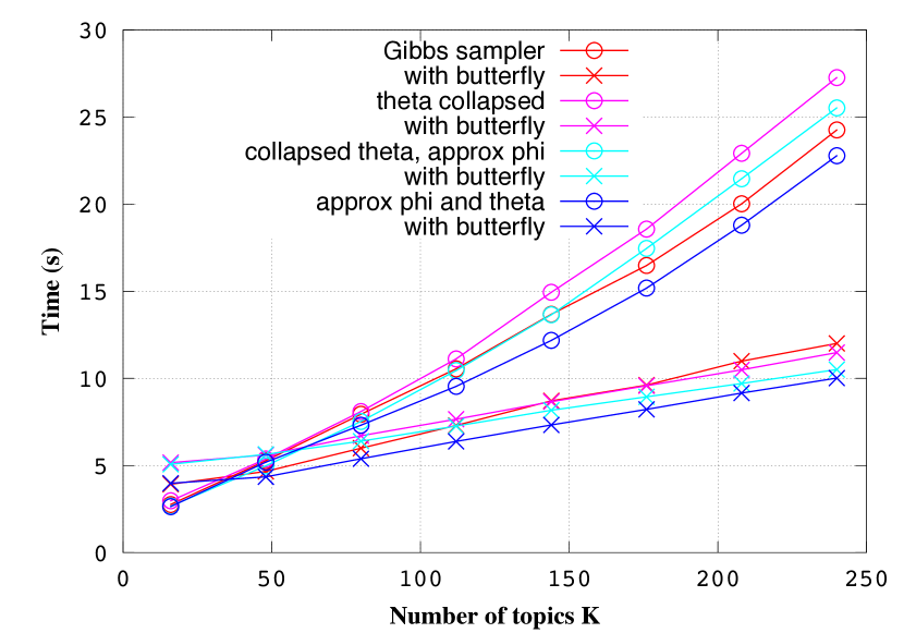
Figure 3: Execution time ($K\mathbin{=}32k+16,0\mathbin{\leq}k\mathbin{\leq}7$)

5 Evaluation

We coded four versions of a complete lda Gibbs-sampler topic-modeling algorithm in cuda for an nvidia Titan Black gpu ($W\mathbin{=}\,32$). For each version we tested two variants, one using Algorithm 1 (using the binary search of Algorithm 3) and one using Algorithm 7. All eight variants were tested for speed using a Wikipedia-based dataset with number of documents $M=43556$, vocabulary size $V=37286$, total number of words in corpus $\Sigma N=3072662$ (therefore average document size $(\Sigma N)/M\approx 70.5$), and maximum document size $\max N=307$. Each variant was measured using eight different values for the number of topics $K$ (16, 48, 80, 112, 144, 176, 208, and 240), in each case performing 100 sampling iterations and measuring the execution time of the entire application, not just the part that draws $z$ values. Best performance requires unrolling three loops in Algorithm 8; we had to manually unroll the loop that starts on line 18, and the cuda compiler then automatically unrolled the loops that start on lines 14 and 20. The performance results are shown in Figure 3. The butterfly variants are faster for $K\geq 80$. For $K\geq 200$, for each of the four versions the butterfly variant is more than twice as fast.

6 Related Work

Because the computed probabilities are relative in our LDA application, it is necessary to compute all of them and then to compute, if nothing else, their sum, so that the relative probabilities can be effectively normalized. Therefore every method for drawing from a discrete distribution represented by a set of relative probabilities involves some amount of preprocessing before drawing from the distribution. The various algorithms in the literature have differing tradeoffs according to what technique is used for preprocessing what technique is used for drawing; some algorithms also accommodate incremental updating of the relative probabilities by providing a technique for incremental preprocessing.

Instead of doing a binary search on the table of partial sums, one can instead (as Marsaglia Marsaglia-1963 observes in passing) construct a search tree using the principles of Huffman encoding Huffman-1952 (independently rediscovered by ZimmermanZimmerman-1959 ) to minimize the expected number of comparisons. In either case the complexity of the search is $O(\log n)$, but the optimized search may have a smaller constant, obtained at the expense of a preprocessing step that must sort the relative probabilities and therefore have complexity $\Omega(n\log n)$.

Walker Walker-arbitrary-1974 ; Walker-TOMS-1977 describes what is now known as the “alias” method, in which $n$ relative probabilities are preprocessed into two additional tables $F$ and $A$ of length $n$. To draw a value from the distribution, let $k$ be a integer chosen uniformly at random from $\{0,1,2,\ldots,n-1\}$ and let $u$ be chosen uniformly at random from the real interval $[0,1)$. Then the value drawn from the distribution is

$$\mathbf{if}\;u<F_{k}\;\mathbf{then}\;k\;\mathbf{else}\;A_{k}$$

Therefore, once the tables $F$ and $A$ have been produced, the complexity of drawing a value from the distribution is $O(1)$, assuming that the cost of an array access is $O(1)$. Walker’s method Walker-TOMS-1977 for producing the tables $F$ and $A$ requires time $\Theta(n^{2})$; it is easy to reduce this to $\Omega(n\log n)$ by sorting the probabilities [KNUTH-VOLUME-2, , exercise 3.4.1-7] and then using, say, priority heaps instead of a list for the intermediate data structure. Either version heuristically attempts to minimize the probability of having to access the table $A$.

Vose Vose-1991 describes a preprocessing algorithm, with proof, that further reduces the preprocessing complexity of the alias method to $\Theta(n)$. The tradeoff that permits this improvement is that the preprocessing algorithm makes no attempt to minimize the probability of accessing the array $A$.

Matias et al. Matias-1993 describe a technique for preprocessing a set of relative probabilities into a set of trees, after which a sequence of intermixed generate (draw) and update operations can be performed, where an update operation changes just one of the relative probabilities; a single generate operation takes $O(\log^{*}n)$ expected time, and a single update operation takes $O(\log^{*}n)$ amortized expected time.

Li et al. li_reducing_14 describe a modified LDA topic modeling algorithm, which they call Metropolis-Hastings-Walker sampling, that uses Walker’s alias method but amortizes the cost of constructing the table by drawing from the same table during multiple consecutive sampling iterations of a Metropolis-Hastings sampler; their paper provides some justification for why it is acceptable to use a “slightly stale” alias table (their words) for the purposes of this application.

7 Conclusions

The technique of constructing butterfly-patterned partial sums appears to be best suited for situations where a SIMD processor is used to compute tables of relative probabilities for multiple discrete distributions, each of which is then used just once to draw a single value, and where each thread, when computing its table, must fetch data from a contiguous region of memory whose address is computed from other data. The LDA application for which we developed the technique has these characteristics. The technique uses transposed memory access in order to allow a SIMD memory controller to touch only one or two cache lines on each fetch, then cheaply constructs a set of partial sums that are just adequate to allow partial sums actually needed to be constructed on the fly during the course of a binary search. For a complete lda Gibbs-sampler topic-modeling algorithm coded in cuda for an nvidia Titan Black gpu and already tuned as best we could for high performance, the butterfly-patterned partial-sums technique further improves the speed of the overall application by at least a factor of 2 when the number of topics is greater than 200.

References

- [1] Christopher M. Bishop. Pattern Recognition and Machine Learning (Information Science and Statistics). Springer-Verlag New York, Inc., 2006.
- [2] David M. Blei. Probabilistic topic models. Commun. ACM, 55(4):77–84, April 2012. \hrefhttp://dx.doi.org/10.1145/2133806.2133826 \pathdoi:10.1145/2133806.2133826.
- [3] David M. Blei, Andrew Y. Ng, and Michael I. Jordan. Latent Dirichlet allocation. J. Machine Learning Research, 3:993–1022, March 2003. URL: \urlhttp://dl.acm.org/citation.cfm?id=944919.944937.
- [4] Thomas L. Griffiths and Mark Steyvers. Finding scientific topics. Proc. National Academy of Sciences of the United States of America, 101(suppl 1):5228–5235, 2004. \hrefhttp://dx.doi.org/10.1073/pnas.0307752101 \pathdoi:10.1073/pnas.0307752101.
- [5] D.A. Huffman. A method for the construction of minimum-redundancy codes. Proc. IRE, 40(9):1098–1101, Sept 1952. \hrefhttp://dx.doi.org/10.1109/JRPROC.1952.273898 \pathdoi:10.1109/JRPROC.1952.273898.
- [6] S. Lennart Johnsson, Tim Harris, and Kapil K. Mathur. Matrix multiplication on the Connection Machine. In Proc. 1989 ACM/IEEE Conference on Supercomputing, pages 326–332, New York, NY, USA, 1989. ACM. URL: \urlhttp://doi.acm.org/10.1145/76263.76298.
- [7] Donald E. Knuth. Seminumerical Algorithms (third edition), volume 2 of The Art of Computer Programming. Addison-Wesley, Reading, Massachusetts, 1998.
- [8] Donald E. Knuth. Sorting and Searching (second edition), volume 3 of The Art of Computer Programming. Addison-Wesley, Reading, Massachusetts, 1998.
- [9] Anthony Lee, Christopher Yau, Michael B. Giles, Arnaud Doucet, and Christopher C. Holmes. On the utility of graphics cards to perform massively parallel simulation of advanced Monte Carlo methods. J. Computational and Graphical Statistics, 19(4):769–789, 2010. URL: \urlhttp://arxiv.org/pdf/0905.2441.pdf.
- [10] Aaron Q. Li, Amr Ahmed, Sujith Ravi, and Alexander J. Smola. Reducing the sampling complexity of topic models. In Proc. 20th ACM SIGKDD International Conference on Knowledge Discovery and Data Mining, KDD ’14, pages 891–900, New York, 2014. ACM. \hrefhttp://dx.doi.org/10.1145/2623330.2623756 \pathdoi:10.1145/2623330.2623756.
- [11] Mian Lu, Ge Bai, Qiong Luo, Jie Tang, and Jiuxin Zhao. Accelerating topic model training on a single machine. In Yoshiharu Ishikawa, Jianzhong Li, Wei Wang, Rui Zhang, and Wenjie Zhang, editors, Web Technologies and Applications (APWeb 2013), volume 7808 of Lecture Notes in Computer Science, pages 184–195. Springer Berlin Heidelberg, 2013. \hrefhttp://dx.doi.org/10.1007/978-3-642-37401-2_20 \pathdoi:10.1007/978-3-642-37401-2_20.
- [12] G. Marsaglia. Generating discrete random variables in a computer. Commun. ACM, 6(1):37–38, January 1963. \hrefhttp://dx.doi.org/10.1145/366193.366228 \pathdoi:10.1145/366193.366228.
- [13] Yossi Matias, Jeffrey Scott Vitter, and Wen-Chun Ni. Dynamic generation of discrete random variates. In Proc. Fourth Annual ACM-SIAM Symposium on Discrete Algorithms, SODA ’93, pages 361–370, Philadelphia, PA, USA, 1993. Society for Industrial and Applied Mathematics. URL: \urlhttp://dl.acm.org/citation.cfm?id=313559.313807.
- [14] NVIDIA. Developer zone website: Cuda toolkit documentation: Cuda toolkit v6.5 programming guide, section B.14. warp shuffle functions, 2015. Online documentation. Accessed February 6, 2015. URL: \urlhttp://docs.nvidia.com/cuda/cuda-c-programming-guide/index.html#warp-shuffle-functions.
- [15] Marc A. Suchard, Quanli Wang, Cliburn Chan, Jacob Frelinger, Andrew Cron, and Mike West. Understanding GPU programming for statistical computation: Studies in massively parallel massive mixtures. J. Computational and Graphical Statistics, 19(2):419–438, 2010.
- [16] Jean-Baptiste Tristan, Daniel Huang, Joseph Tassarotti, Adam C. Pocock, Stephen Green, and Steele, Guy L., Jr. Augur: Data-parallel probabilistic modeling. In Z. Ghahramani, M. Welling, C. Cortes, N. D. Lawrence, and K. Q. Weinberger, editors, Advances in Neural Information Processing Systems 27, pages 2600–2608. Curran Associates, Inc., 2014. URL: \urlhttp://papers.nips.cc/book/year-2014.
- [17] M.D. Vose. A linear algorithm for generating random numbers with a given distribution. IEEE Trans. Software Engineering, 17(9):972–975, Sept 1991. \hrefhttp://dx.doi.org/10.1109/32.92917 \pathdoi:10.1109/32.92917.
- [18] A. J. Walker. New fast method for generating discrete random numbers with arbitrary frequency distributions. Electronics Letters, 10(8):127–128, April 1974. \hrefhttp://dx.doi.org/10.1049/el:19740097 \pathdoi:10.1049/el:19740097.
- [19] Alastair J. Walker. An efficient method for generating discrete random variables with general distributions. ACM Trans. Math. Software, 3(3):253–256, September 1977. \hrefhttp://dx.doi.org/10.1145/355744.355749 \pathdoi:10.1145/355744.355749.
- [20] Nicholas Wilt. The CUDA Handbook: A Comprehensive Guide to GPU Programming. Addison-Wesley, Upper Saddle River, New Jersey, 2013.
- [21] Feng Yan, Ningyi Xu, and Yuan Qi. Parallel inference for latent Dirichlet allocation on graphics processing units. In Advances in Neural Information Processing Systems 22, pages 2134–2142. Curran Associates, Inc., 2009. URL: \urlhttp://papers.nips.cc/book/year-2009.
- [22] Huasha Zhao, Biye Jiang, and John Canny. SAME but different: Fast and high-quality Gibbs parameter estimation. CoRR (Computing Research Repository at arXiv.org), September 2014. URL: \urlhttp://arxiv.org/abs/1409.5402.
- [23] Seth Zimmerman. An optimal search procedure. American Mathematical Monthly, 66(8):690–693, Oct 1959.