Abstract

Statistical studies of languages have focused on the rank-frequency distribution of words. Instead, we introduce here a measure of how word ranks change in time and call this distribution rank diversity. We calculate this diversity for books published in six European languages since 1800, and find that it follows a universal lognormal distribution. Based on the mean and standard deviation associated with the lognormal distribution, we define three different word regimes of languages: ‘‘heads’’ consist of words which almost do not change their rank in time, ‘‘bodies’’ are words of general use, while ‘‘tails’’ are comprised by context-specific words and vary their rank considerably in time. The heads and bodies reflect the size of language cores identified by linguists for basic communication. We propose a Gaussian random walk model which reproduces the rank variation of words in time and thus the diversity. Rank diversity of words can be understood as the result of random variations in rank, where the size of the variation depends on the rank itself. We find that the core size is similar for all languages studied.

Introduction

Statistical studies of languages have become popular since the work of George Zipf [1] and have been refined with the availability of large data sets and the introduction of novel analytical models [2, 3, 4, 5, 6, 7]. Zipf found that when words of large corpora are ranked according to their frequency, there seems to be a universal tendency across texts and languages. He proposed that ranked words follow a power law $f\sim 1/k$, where $k$ is the rank of the word—the higher ranks corresponding to the least frequent words—and $f$ is the relative frequency of each word [8, 9]. This regularity of languages and other social and physical phenomena had been noticed beforehand, at least by Jean-Baptiste Estoup [10] and Felix Auerbach [11], but it is now known as Zipf’s law.

Zipf’s law is a rough approximation of the precise statistics of rank-frequency distributions of languages. As a consequence, several variations have been proposed [12, 13, 14, 15]. We compared Zipf’s law with four other models, all of them behaving as $1/k^{a}$ for a small $k$, with $a\approx 1$, as detailed in the SI. We found that all models have systematic errors so it was difficult to choose one over the other.

Studies based on rank-frequency distributions of languages have proposed two word regimes [15, 16]: a ‘‘core’’ where the most common words occur, which behaves as $1/k^{a}$ for small $k$, and another region for large $k$, which is identified by a change of exponent $a$ in the distribution fit. Unfortunately, the point where exponent $a$ changes varies widely across texts and languages, from 5000 [16] to 62,000 [15]. A recent study [17] measures the number of most frequent words which account for $75\%$ of the Google books corpus. Differences of an order of magnitude across languages were obtained, from $2365$ to $21077$ words (including inflections of the same stems). This illustrates the variability of rank-frequency distributions. The core of human languages can be considered to be between 1500 and 3000 words (not counting different inflections of the same stems), based on basic vocabularies for foreigners [18], creole [19], and pidgin languages [20]. For example, Voice of America’s Special English [21] and Wikipedia in Simple English use about 1500 and 2000 words, respectively (not counting inflections). The Oxford Advanced Learner’s Dictionary lists 3000 priority lexical entries [22]. This suggests that the change of exponent $a$ or another arbitrary cutoff in rank-frequency distributions does not reflect the size of the core of languages.

In view of these problems with rank-frequency distributions, we propose a novel measure to characterize statistical properties of languages. We have called this measure rank diversity and it tells us how words change their rank in time. With rank diversity, three regimes of words are identified: ‘‘heads’’, ‘‘bodies’’ and ‘‘tails’’. This measure of rank diversity follows the same simple functional law with similar parameters for all data analyzed. In particular, this is so for the six European languages studied here using a large data set of more than 6.4 $\times 10^{11}$ words from Google Books [23], which contains about $4\%$ of all books written until 2008. It should be noted that this data set includes all different inflected forms (such as plural, different tense/aspect forms, etc.) found in the book corpus. Data sets such as this have allowed the study of ‘‘culturomics’’: how cultural traits such as language have changed in time [24, 25, 26, 27, 28, 29, 30].

The rank diversity follows a scale-invariant behavior regarding its fluctuations, which inspires a model based on random walks, with scale-invariant random steps. This model reproduces the behavior of diversity and thus captures the essence of the evolution of word rank across different languages.

Rank diversity of words

In what follows we shall consider six European languages from the Indo-European family. They are English and German; Spanish, French and Italian; and Russian. They belong to different linguistic branches: Germanic, Romance, and Slavic, respectively. The native speakers of these languages account for approximately 17% of the world population.

We shall start by taking into account the 20, say, most used words in the six languages, that is, the lowest-ranked words. Using, for the sake of uniformity, the first sense or first meaning given by Google Translate, once these words are translated into English, the coincidences in all six languages are remarkable (see Table S1 in File S1). This could have been foreseen, since most of the lowest-ranked words are articles, prepositions or conjunctions, i.e. what is called function words. A different matter, as we shall see, would result if we had considered only nouns, verbs, adverbs or adjectives, known as content words.

In order to quantify this fact, we present in Fig. 1 the time evolution of the overlap of the first 20 lowest-ranked words in the five languages with respect to the corresponding list of English. From the upper part of this figure we can see that along two centuries this overlap fluctuates around 0.9, a rather large number, except for Russian, since this language does not have articles. These data reveal that these Indo-European languages have shared structural properties, notwithstanding that they belong to distinct linguistic branches.

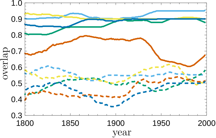
Figure 1: Overlap of the 20 most frequent words (continuous lines), and of the 20 most frequent content words (dashed lines) across languages, with respect to English, as a function of time. When words have more than one meaning, the first sense, according to Google Translate, was used. The color code for languages is as follows: light blue for French, green for German, yellow for Italian, dark blue for Spanish, and dark orange for Russian. Additionally, light orange will be used for English when required (see also Fig. 2). The same color coding for languages will be used throughout the rest of the article.

The lowest-ranked words used to construct the upper part of Fig. 1 are essentially the same along centuries (See Figs S3-S8 in SI). But this is not the case for content words, as can be seen in Table S2 in File S1. First, and as also shown by the dashed curves in Fig. 1, the overlap of these words with respect to English for the other five languages (including Russian) is of the order of 0.5. These values are much lower than the overlap of function words. Second, the most common nouns vary considerably with time. On the one hand, nouns like time, man, life and their translation to the other languages are present independently of the century. On the other hand, words like god and king have a low rank in the eighteenth century but have a larger rank in the last century. The rank change in time of these nouns reflect cultural facts.

What is discussed in the previous paragraph is an example of what could be called rank diversity $d(k)$. This is, in the present study, the number of different words occurring at a specific rank $k$ over a given period of time $\Delta t$. We found that the resulting rank diversity curves for the six languages studied between 1800 and 2008 are similar to each other, as shown in Figs. 2 and 6. Low ranks have a very low diversity, as few words appear in the same ranks for the years we have studied.

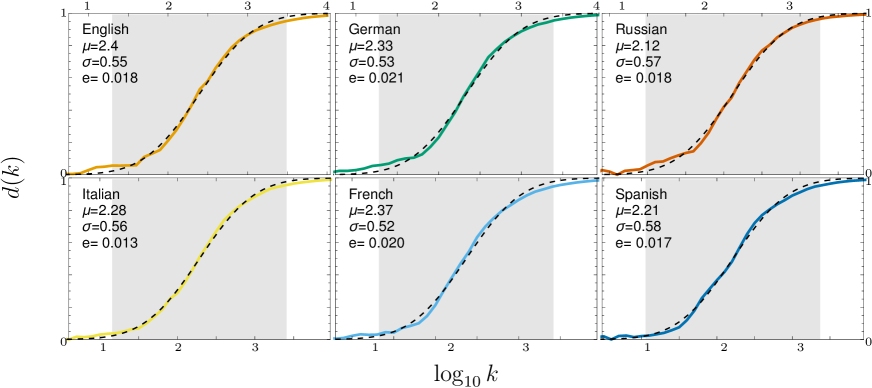
Figure 2: Rank diversity. Diversity $d$ as a function of the rank $k$ for different languages from 1800 to 2008, where $d(k)$ measures how many different words appear for a given rank $k$ during the time considered ($\Delta t=208$). For example, for English, $d(1)=1/208$, as the word ‘the’ appears in the first rank for all years considered. Although we have analyzed up to $k\approx 10^{6}$, rank diversity for $k>10^{4}$ is not shown as $d(k)\approx 1$, i.e., a different word appears in each rank every year. Data are windowed over time, with a slot of size $\delta\log_{10}k=0.1$, for the sake of clearness. Additionally, the sigmoid defined in equation 1 is shown as a black dashed curve, with the best fit parameters, also reported in each subfigure. The mean square error $e$ between the data and the fit, is also given. The shaded region corresponds to the average ‘‘body’’ of all languages.

As shown by the continuous lines in Fig. 2, the sigmoid curve fits very well $d(k)$ for all languages considered, except for low $k$ where the statistical fluctuations are larger due to the small sample size. The sigmoid is the cumulative of a Gaussian distribution, i.e.

$$\Phi_{\mu,\sigma}(\log_{10}k)=\frac{1}{\sigma\sqrt{2\pi}}\int_{-\infty}^{\log_{10}k}\mathrm{e}^{-\frac{(y-\mu)^{2}}{2\sigma^{2}}}{\rm d}y,$$ (1)

and is given as a function of $\log k$. The values of $\mu$ and $\sigma$ reported in Fig. 2 were obtained adjusting equation 1 to the rank diversity calculated for each individual language. The mean value $\mu$ identifies the point where $d(k)\approx 0.5$, while the width $\sigma$ gives the scale in which $d(k)$ gets close to its extremal values. When $\log k$ is much larger than $\mu+\sigma$, $\Phi_{\mu,\sigma}(\log k)$ gets exponentially close to one, whereas when $\log k$ is much smaller than $\mu-\sigma$ it gets exponentially close to zero. It is customary in statistics to define a bulk of the Gaussian between $\mu\pm 2\sigma$, where 95% of the population lies. Along the same lines, we define three regions, marked by

$$\log_{10}k_{\pm}=\mu\pm 2\sigma.$$ (2)

First, we find what we shall call the head of the language, distributed with ranks between 1 and $k_{-}$; a second region, identified as the body of the language, lies between $k_{-}$ and $k_{+}$; and finally the tail, beyond $k_{+}$. From the values reported in Fig. 2, we see that $9<k_{-}<22$, while $k_{+}$ lies between $1832$ and $3099$. As shown in Fig. 3, these regions are robust to changes in the historical period considered and to the data set size (larger for recent years).

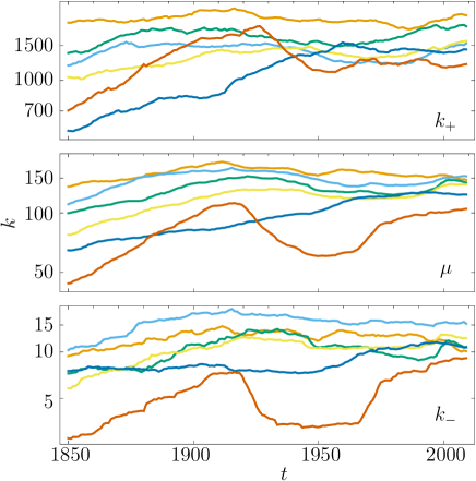
Figure 3: Evolution in time of the center of the sigmoid (middle panel), and the borders of the head and body (bottom panel) and body and tail (top panel) for the different languages along time for intervals of fifty years, i.e. $\Delta t=50$. Head words have $k\leq k_{-}$, body words have $k_{-}<k\leq k_{+}$, and tail words have $k_{+}<k$. See Fig. 2 for color coding.

The bodies of languages consist of words that have limited change in time. Based on the size of basic vocabularies, it can be argued that the ‘‘core’’ of English is between 1500 and 3000 words, as mentioned in the introduction, which is consistent with our results. If we agree that the rank diversity identifies the core (head and body) of English, then it can be argued that the size of the core of the other five languages studied is similar [31], which is also supported by the high similarity across languages in Fig 2.

The tails of languages are formed by words which vary their rank considerably in time. This implies that they are more dependent on the text and its domain than words from the core. It can be assumed that words belonging to the head and body of languages have a high probability of being used in any text, while words from the tail would appear only in specific texts and domains.

Note that we obtain language cores slightly larger than those proposed by linguists. This is to be expected, as the Google Books data set treats words forms inflected for different persons, tenses, genders, numbers, cases, and so forth, as distinct items, while dictionaries count only stems (presented as citation forms, i.e. the basic form that users are most likely to look up). For example, the core for English obtained using rank diversity consists of 2448 words, but within these there are only 1760 different stems in the year 2008. Moreover, the studied data set contains several proper names which are not included in basic vocabulary lists. For English, 55 out of 2448 are proper names in 2008.

The rank evolution of particular words in time, belonging to the head, body, and tail of English is shown in Fig. 4. This ratifies the results shown in Fig. 2, where low-ranked words exhibit little variation in time and this variation increases with the rank. More trajectories are presented in the SI. As mentioned above, words from the head vary little over time. However, the way in which words from the body or tail vary their rank in time appears to be similar, although at a different scale. This similarity leads us to propose a model of rank diversity where the amount of rank variation depends only on the rank.

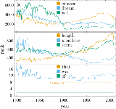
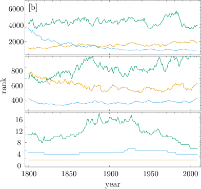
Figure 4: Rank evolution. [a]: Evolution of the rank for several particular, but random words in different regimes in the English language. From bottom to top we show words with initial ranks of order $1$ (head), $100$ (body) and $1000$ (tail). [b]: Evolution of the rank for several particular, but random words in different regimes, for our scale-free Gaussian walker, i.e. the simulated language we have generated.

A random walk model for rank diversity

We consider the relative size of frequency changes, or flights as they are sometimes called in statistical physics, defined as $\left(k_{t+1}-k_{t}\right)/k_{t}$ where $k_{t}$ is the rank at discrete time $t$ of a given element. We present in Fig. 5 the distribution of these frequency changes for English, our largest data set, and in Fig. 17 in File S1 for all languages. Notice that, on average, the relative jumps seem to be largely independent of the value of the rank. We propose, based on this fact, a simple model to understand the evolution of rank diversity of words.

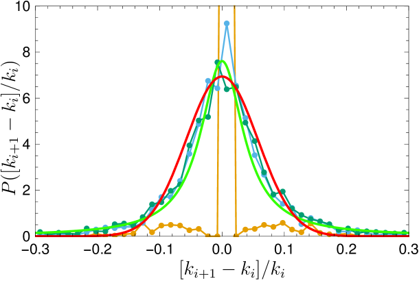
Figure 5: Distribution of relative size of frequency changes $[k_{t+1}-k_{t}]/k_{t}$ in the case of English for words in the head $\blacksquare$ (that start with rank between 1 and 10), the body $\blacksquare$ (rank between 200 and 210), and the tail $\blacksquare$ (rank between 5000 and 5010). Notice that for words in the head, the granularity of the model (equation 3) shows up as large deviations from the Gaussian. For the body and tail, the relative jumps are similar independently of the initial rank of the word. We also show, as a thick green curve, the Lorentzian distribution which best fits the average of the curves for the body and tail. A Gaussian, with zero mean and the most common standard deviation $\hat{\sigma}=0.0575$, is also shown in red for comparison (see text for details). The corresponding plot for other languages is shown in the supplementary information.

We shall call this model a scale-invariant random Gaussian walk, since a word with rank $k_{t}$, is converted to rank $k_{t+1}$ according to the following procedure: One defines an auxiliary variable $s_{t+1}$ at time $t+1$ by the relation

$$s_{t+1}=k_{t}+G\left(0,k_{t}\hat{\sigma}\right),$$ (3)

where $G(0,\tilde{\sigma})$ is a Gaussian random number generator of width $\tilde{\sigma}$ and mean $0$. This means that the random variable $s_{t+1}$ has a width distribution proportional to $k_{t}$. Words with very low ranks will change very slowly or not at all, while those with higher $k$ have a larger rank variation in time, as reflected by $d(k)$. Once the values of $s_{t+1}$ for all words are obtained, they are ordered according to their magnitude. This new order gives new rankings, i.e. the $k$ values at time $t+1$. There is a small correlation of the jumps between different times in this model. This is consistent with the observed behavior of the six languages dealt with here, as can be seen in Fig. 18 in File S1. The only parameter in the model is the width $\hat{\sigma}$, which is the most common standard deviation of the relative frequency changes of each data set.

A word of caution must be said. In Fig. 5, two curves are plotted. In green, a Lorentzian distribution, and in red a Gaussian distribution, both centered at zero, and with a width obtained by best fit to the data presented here. Although the Lorentzian fits these data somewhat better than the Gaussian, we use the latter in our model, since the long tails of the Lorentzian would yield long flights in words (not observed in the historical data) and a very different function $d(k)$. One should recall that the Lorentzian does not have a finite second moment, so this might be the reason for this distribution to be inadequate. It is probable that a truncated Lorentzian could be a better choice, but we leave this detail open as a possible refinement to our model.

With this model we have produced the evolution of a random simulated language; see [32] for other approaches. Fig. 4 shows examples of rank trajectories at different scales, exhibiting similarities with those of actual words shown in Fig. 4. Moreover, if its diversity $d(k)$ is calculated with the $\hat{\sigma}$ corresponding to the most popular width of the distribution of relative size of flights for all words in the English language from 1800 to 2008, the results coincide with the sigmoid obtained for all six languages analyzed, as shown in Fig. 6.

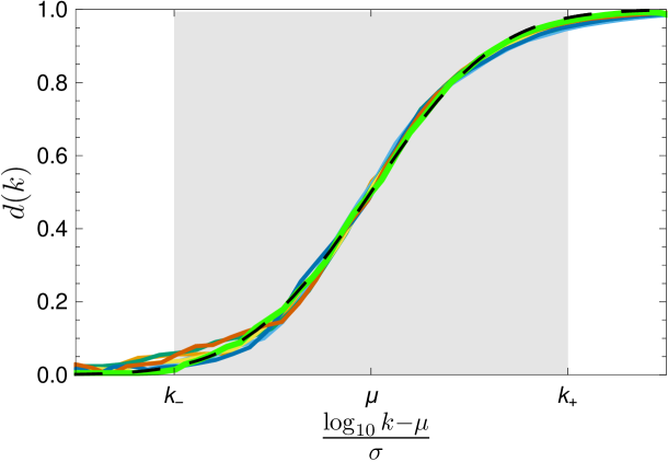
Figure 6: Rank diversity for the simulated language. The green curve represents the diversity corresponding to the language dynamics of a single realization of the Gaussian random walk model. We also include data for all languages studied, but normalized so that $k_{\pm}$ coincide. The ansatz for the rank diversity is plotted as a parameter-free cumulative of a Gaussian with zero mean and unit variance as a dashed black curve.

Discussion

Within statistical linguistics, the frequency-rank distributions of several languages of European origin have been analyzed for many years now. However, no simple model can reproduce the detailed properties of this distribution (see SI). In particular, there has been the proposal that there exist two different regimes for ranks, but these regimes have not been satisfactorily validated in the empirical data. Due to these difficulties we have been led to introduce a statistical measure, which we have called rank diversity, to describe the statistical properties of natural languages. A simulated random language was generated which reproduces the observed features quite well.

Our random walk model mimics the evolution of languages to produce a simulated rank diversity which closely matches that of historical data. We consider that statistical similarities across languages and the simplicity of the model to reproduce them sufficient evidence to claim that rank diversity of words is universal. This does not imply that all languages have the same rank diversity curves, but that the rank diversity distribution of all the languages studied here can be fitted properly with equation 1. Certainly, different languages have different curves that fit them better, just as different exponents fit better a Zipf distribution of different languages. For the languages studied, $1.6\leq\mu\leq 2.1$ and $0.4\leq\sigma\leq 0.6$.

This universality could be used to favor nativist explanations of human language [33, 34], where language is claimed to be determined by innate constraints. However, the high-ranked diversity of language tails could be used in favor of adaptationist explanations as well [35], as the precise rank of tail words is highly contingent. In recent years, explanations of human language relating biological evolution (genetically encoded innate properties) and learning (epigenetical adaptation) with culture have gained strength [36, 37, 38]. Even so, few assumptions are necessary to explain some general aspects of the evolution of human languages [39]. The present work shows that the evolution of word frequency can be explained with Gaussian random walks, where the size of the change in word frequency is proportional to its rank, i.e. frequent words change less than infrequent words. This explanation does not require innate properties, adaptive advantages, nor culture. This does not imply that the latter are irrelevant for other aspects of language evolution. Note that our study is carried out at a statistical level. We do not address syntactic, semantic, and grammatical aspects of human language [40, 41, 42, 43], which are certainly important.

Why does the rank diversity approach a lognormal distribution? Which processes and mechanisms are required for this? There is one condition for a variable to have a lognormal distribution. This condition is that the variable should be the result of a high number of different and independent causes which produce positive effects composed multiplicatively. Thus, each cause has a negligible effect on the global result [44]. Our Gaussian random walk model supports this as a suitable explanation: the statistical distribution of $d$ is always lognormal, there is a high number of components (words), each word has a negligible effect compared to the language properties, i.e. large changes in word frequency (ranking) do not cause large changes in the statistical properties of each language, and the rank of each word is partially a cumulative product of its rank in previous times, as expressed in equation 3. Languages statistically comply with these dynamics, and that serves as an explanation for their evolution and structure.

In future work, it will be relevant to study the rank diversity of $n$-grams with $n>1$ [45], other linguistic corpora and phenomena with dynamic rank distributions [27, 46, 47, 48] and more generally with temporal networks [49, 50, 51, 52]. A specific example would be the ranking of chess players, given by the World Chess Federation (Fédération Internationale des Échecs). The rank diversity in this case is provided in figure 7, which shows that the sigmoid is appropriate also for this case.

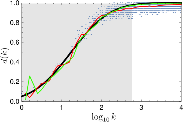
Figure 7: Rank diversity of male chess players obtained from the trimestral FIDE rankings from April, 2001 to May, 2012 ($\Delta t=50$), considering the first 10,000 ranks. Blue dots show rank diversity, windowed in the red line. The black line shows the sigmoid fit with $\mu=1.24$ and $\sigma=0.76$. The green line shows a simulation with $\hat{\sigma}=0.18$. Notice that there is no head as $\mu-2\sigma<0$. This is to be expected, as many players enter and leave the ranking during the years considered.

Supporting Information

S1 Models for rank-frequency distributions

The rank-frequency distributions of words for different languages are very similar to each other, as shown in Fig. 8. The distributions are also similar across centuries, as shown in Fig. 8.

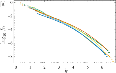
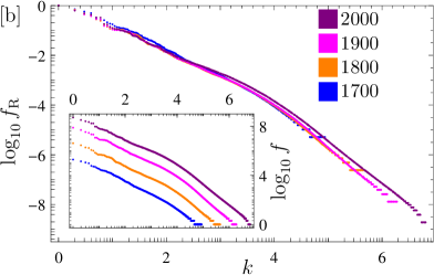
Figure 8: Rank distributions of words according to frequency. [a]: Normalized word frequency $f_{\textup{R}}$ as a function of the rank $k$ for several languages for books published in the year 2000. The color code for languages is as follows: $\blacksquare$ for French, $\blacksquare$ for German, $\blacksquare$ for Italian, $\blacksquare$ for English, $\blacksquare$ for Spanish, and $\blacksquare$ for Russian. [b]: Word frequency $f_{\textup{R}}$ as a function of the rank $k$ for English and several years, normalized so that the most frequent element has relative frequency one. In the inset, the unnormalized frequency $f$ is shown.

We present five different distributions with distinct origins, though all of them containing the common factor $\frac{1}{k^{a}}$. The distributions are:

$$m_{1}(k) =\mathcal{N}_{1}\frac{1}{k^{a}},$$ (S4)

$$m_{2}(k) =\mathcal{N}_{2}\frac{\mathrm{e}^{-b(k-1)}}{k^{a}},$$ (S5)

$$m_{3}(k) =\mathcal{N}_{3}\frac{(\bar{N}+1-k)^{\alpha}}{k^{a}},$$ (S6)

$$m_{4}(k) =\mathcal{N}_{4}\frac{(\bar{N}+1-k)^{\alpha}\mathrm{e}^{-b(k-1)}}{k^{a}},$$ (S7)

$$m_{5}(k) =\mathcal{N}_{5}\begin{cases}\frac{1}{k}&k\leq k_{c}\\ \frac{k_{c}^{a-1}}{k^{a}}&k>k_{c}\end{cases}$$ (S8)

where $\mathcal{N}_{i}$ are normalization factors, depending on the parameters $a$, $b$, and $\alpha$ of the different models, and $\bar{N}$ is the total number of words.

In Fig. 9 we compare the fit of these distributions with the observed curves. It can be seen that none of the distributions reproduces closely the dataset. We calculated for all fits the $\chi^{2}$ test with similar results. The best value corresponds to the fit proposed in [15], namely the double Zipf model (equation (S8)). In all cases we studied the $p$-value of the data, needed for an appropriate interpretation of the goodness of the fit. In all cases, that is for all years, all languages and all models, this number was smaller than machine precision. This shows that none of these models captures satisfactorily the data behavior.

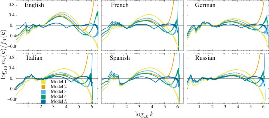
Figure 9: Comparison between the different models, equation (S4)–equation (S8), and the frequency of rank distribution. We use the data for the year 2000 and all languages under consideration. The logarithm base 10 of the ratio of the observed values and the model is plotted. It can be appreciate that different models fit better in different regions. However there is no model that fits all languages and all regions much better than the others.

The origin of some of these models is similar. The following discussion shows how they can be encompassed in a common formulation.

Given a set of words forming a text, one can evaluate the number of times $N(k,t)$ that a certain word appears with the rank $k$ at time $t.$ If $B(k)$and $D(k)$ denote, respectively, the probability per unit time that a word enters or leaves the rank $k$, we have:

$$\frac{\partial}{\partial t}N(k,t)=\left\{\xi(k)-F[\Sigma(t)]\right\}N(k,t)\\ +\Big{\{}D(k+1)N(k+1,t)+B(k-1)N(k-1,t)-\left[D(k)+B(k)\right]N(k,t)\Big{\}}.$$ (S9)

Here the two terms on the r.h.s. within the first curly brackets describe, respectively, the local growth rate and the overall decrease rate acting on $N(k,t).$ The total number of words at a given time $t$ is $\Sigma(t)$ and $F$ is a function that determines global constraint features that refer to the total number of words. The terms within the second curly brackets, indicate the balance arising from the birth $B(k)$ and death $D(k)$ contributions of first neighbor words with $k\pm 1$ ranks at time $t$. If we consider the total number of words at a given time $t$ to be a fixed quantity,

$$\Sigma(t)=\sum_{k}N(k,t)$$ (S10)

we can define the probability density of finding a word with rank $k$, or relative frequency distribution, by

$$n(k,t)\equiv\frac{N(k,t)}{\Sigma(t)}.$$ (S11)

Substitution of equation (S10) and equation (S11) into equation (S9) leads to

$$\frac{d}{dt}\Sigma(t)=\langle\xi(k)\rangle-F[\Sigma(t)]\Sigma(t),$$ (S12)

where the bracket indicates a sum over all $k$ weighted by $n(k,t).$ We assume, for simplicity, that $\langle\xi(k)\rangle$ is a linear function of the number of edges $k$, so that $\langle\xi(k)\rangle$ = $\xi_{0}+\xi_{1}\langle k\rangle,$ where $\xi_{0}$ and $\xi_{1}$ are constants. Then equation (S9) reduces to the following master equation for a one step process:

$$\dot{n}(k,t)=V(k)n(k,t)\\ +\left\{D(k+1)n(k+1,t)+B(k-1)n(k-1,t)-\left[D(k)+B(k)\right]n(k,t)\right\},$$ (S13)

where $\dot{n}(k,t)\equiv\partial n(k,t)/\partial t$ and the effective potential $V(k)\equiv\xi(k)-\langle\xi(k)\rangle$ has the property

$$\langle V(k)\rangle=0.$$ (S14)

In what follows we shall only consider the case $\xi(k)=\xi_{0},$ so equation (S13) reduces to the general form of the master equation for a one step process,

$$\dot{n}\left(k,t\right)=D\left(k+1\right)n\left(k+1,t\right)+B\left(k-1\right)n\left(k-1,t\right)-\left[D(k)+B(k)\right]n(k,t).$$ (S15)

If the changes in $k$ are small and we are only interested in solutions $n\left(k,t\right)$ that vary slowly with $k$, then $k$ may be treated as a continuous variable and we obtain the Fokker-Planck equation:

$$\frac{\partial n\left(k,t\right)}{\partial t}=-\frac{\partial}{\partial k}\left[g\left(k\right)n\left(k,t\right)\right]+\frac{1}{2}\frac{\partial^{2}}{\partial k^{2}}\left[f\left(k\right)n\left(k,t\right)\right],$$ (S16)

where $f(k)=B(k)+D(k)$ and $g(k)=B(k)-D(k)$. For the stationary solutions $m(k)$, we have the equation

$$g(k)m(k)=\frac{1}{2}\frac{d}{dk}\left[f(k)m(k)\right].$$ (S17)

If we approximate $g(k)/f(k)$ by Padé approximants $g_{n}(k)/f_{n}(k)=A_{0}+\sum_{k=1}^{n}\frac{A_{k}}{(k+c_{k})}$, the stationary solution becomes

$$m(k)=\mathcal{N}\textrm{exp}\left(A_{0}k\right)\prod_{k=1}^{n}(k+c_{k})^{-A_{k}}.$$ (S18)

If we assume the simplest expression for $D(k)$ and $B\left(k\right)$ transition probabilities

$$D(k) =\lambda_{1}(c_{1}+k)(N_{1}-k),$$ (S19)

$$B(k) =\lambda_{2}(c_{2}+k)(N_{2}-k)$$ (S20)

then

$$m(k)=\mathcal{N}\textrm{exp}(A_{0}k)\frac{\left(\bar{N}-k\right)^{b}}{(\bar{c}+k)^{a}},$$ (S21)

where $\bar{N}=\frac{1}{2}\left(N_{1}+N_{2}\right)$, $\bar{c}=\frac{1}{2}\left(c_{1}+c_{2}\right)=1$, $a=c_{1}-c_{2}+1$, and $b=N_{1}-N_{2}-1$. Also we must remember that in our case $k$ starts at one. Then if $A_{0}=b=0,$ we have the Zipf model; when $A_{0}\neq 0$ and $b=0,$ the $\gamma$ model is gotten (equation (S5)); if $A_{0}=0$ but $b\neq 0$ the $\beta$ model is obtained (equation (S6)); finally, if $A_{0}$ and $b$ are different from 0, we have the general $\beta\gamma$ model (equation (S7)).

These and additional results could be obtained using the complex network language [53, 54, 55].

With respect to the distribution of equation (S8), the derivation given in [15] is based on the following assumptions. The existence of two word regimes: A language core containing words with low rank and do not affect the birth of new words, and the remaining high ranked words which reduce the probability of new words to be used.

S2 Variation of words in time

Table S1 shows the most frequent words for the year 2000 with their translation and relative frequency. Notice that these are very similar across languages. Table S2 shows the most frequent nouns for the years 1700, 1800, 1900, and 2000. There are similarities across languages and across centuries, but also important differences.

Table 1: Lowest–rank words for several languages in books published during the year 2000, together with their translation to English and their relative frequency.

rank	English	German	French	Italian	Spanish	Russian
1	the, 0.065530	der, the, 0.038512	de, of, 0.057225	di, of, 0.041518	de, of, 0.073063	и, and, 0.053961
2	of, 0.036769	die, the, 0.036010	la, the, 0.035222	e, and, 0.028107	la, the, 0.043297	в, in, 0.053922
3	and, 0.029289	und, and, 0.028087	et, and, 0.024466	la, the, 0.020308	en, in, 0.029059	на, on, 0.020190
4	to, 0.025264	in, in, 0.020607	le, the, 0.022384	che, that, 0.017861	y, and, 0.028908	не, not, 0.017334
5	in, 0.021769	von, of, 0.011277	les, the, 0.021076	il, the, 0.017702	el, the, 0.027771	что, what, 0.011770
6	a, 0.020715	den, the, 0.011012	à, to, 0.019951	in, in, 0.017357	que, that, 0.026713	по, by, 0.010202
7	is, 0.010712	zu, to, 0.010488	des, of, 0.019212	a, to, 0.014067	a, to, 0.019706	к, to, 0.008559
8	that, 0.010529	des, of, 0.010102	en, in, 0.014334	del, of, 0.013403	los, the, 0.018039	как, as, 0.008027
9	for, 0.008975	das, the, 0.009806	du, of, 0.012991	della, of, 0.010876	del, of, 0.013492	а, and, 0.007745
10	as, 0.007396	im, in the, 0.007418	un, a, 0.011112	per, for, 0.010480	se, oneself, 0.012448	о, about, 0.006824
11	it, 0.006832	mit, with, 0.007403	une, a, 0.010825	un, a, 0.009949	las, the, 0.012294	из, of, 0.006356
12	with, 0.006707	sich, itself, 0.007337	dans, in, 0.010145	non, not, 0.008645	por, by, 0.009908	его, his, 0.005911
13	was, 0.006576	ist, is, 0.007197	que, that, 0.009896	si, oneself, 0.008515	un, a, 0.008824	для, for, 0.005822
14	on, 0.006289	auf, on, 0.007047	qui, who, 0.008609	è, is, 0.008501	con, with, 0.008469	от, from, 0.005769
15	not, 0.005970	nicht, not, 0.006875	par, by, 0.007494	una, a, 0.007891	una, a, 0.007863	он, he, 0.005538
16	be, 0.005671	für, for, 0.006874	est, is, 0.007258	le, the, 0.007852	no, no, 0.007547	но, but, 0.005324
17	by, 0.005440	eine, a, 0.006757	pour, for, 0.007027	i, the, 0.007626	para, for, 0.006877	я, I, 0.005097
18	i, 0.005212	als, as, 0.006521	il, it, 0.006749	con, with, 0.006734	su, its, 0.006597	это, this, 0.004925
19	are, 0.004928	dem, the, 0.005723	au, to the, 0.006429	da, from, 0.006258	es, is, 0.006086	за, for, 0.004623
20	this, 0.004916	auch, also, 0.005630	a, has, 0.005504	nel, in, 0.005184	al, to the, 0.005855	у, at, 0.003862

Table 2: Lowest ranked nouns for different years (top left cell) and different languages. Note that some words are used not only as nouns, which can give them a higher rank. For example, été in French is summer, but also the past participle of être (to be).

English German French Italian Spanish Russian 1 time Nichts, nothing fait, fact era, era dios, god время, time 2 king Zeit, time point, point parte, part parte, part году, year 3 man Art, type été, summer tempo, time tiempo, time день, day 4 god Derselben, the same eau, water prima, first solo, single года, year 5 first Menschen, people partie, part stato, state señor, mr. времени, time 6 part Allein, alone corps, body città, city hombre, man людей, people 7 men Natur, nature temps, time repubblica, republic cuerpo, body города, city 8 general — terre, land cose, things vida, life образомъ, way 9 people — nombre, number fatto, fact modo, mode земли, land 10 place — homme, man luogo, place hombres, men будетъ, will 1900 English German French Italian Spanish Russian 1 time Selbst, even été, summer era, era señor, mr. время, time 2 man Jahre, years fait, fact parte, part parte, part года, year 3 first Weise, wise point, point stato, state ley, law жизни, life 4 life Ersten, first temps, time legge, law gobierno, government времени, time 5 men Recht, right cas, case prima, first estado, state образомъ, way 6 day Art, type droit, right fatto, fact derecho, right будетъ, will 7 old Einzelnen, individual loi, law tempo, time años, years томъ, volume 8 years Frage, question partie, part vita, life año, year году, year 9 work Nichts, nothing Paris, Paris anni, age ciudad, city права, right 10 people — France, France Italia, Italy artículo, article право, right 2000 English German French Italian Spanish Russian 1 time Deutschen, German fait, fact era, era parte, part время, time 2 first Jahre, years été, summer parte, part años, years old том, volume 3 people Menschen, people paris, Paris stato, state estado, state года, year 4 work Frage, question temps, time prima, first vida, life федерации, federation 5 way Deutschland, Germany pays, country anni, years años, years жизни, life 6 life Jahren, years politique, policy vita, life nacional, national лет, years 7 world Berlin, Berlin vie, life tempo, time tiempo, time человек, man 8 way Ersten, first france, France secondo, second social, social году, year 9 state Entwicklung, development travail, work modo, way forma, form раз, time 10 years Arbeit, work monde, world fatto, fact política, policy человека, human

Figs. 10–16 show rank trajectories of words for the languages studied, including our simulated language. It can be seen that the behavior is similar for all languages: words with low rank (heads) almost do not vary in time. Afterwards the variation in rank depends on the rank itself, approximating a scale-invariant random walk. Notice that there is a higher variation at all scales before 1850. Further work is required to measure how much this variation depends on having less data before 1850 and how much on language properties of the time.

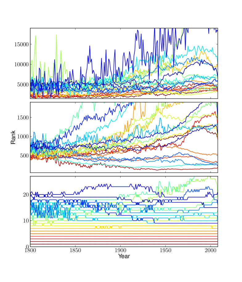
Figure 10: Rank variations in time of twenty words from three different scales for English.

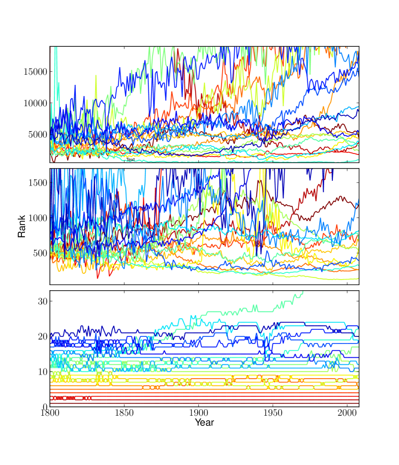
Figure 11: Rank variations in time of twenty words from three different scales for German.

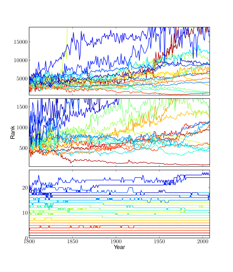
Figure 12: Rank variations in time of twenty words from three different scales for French.

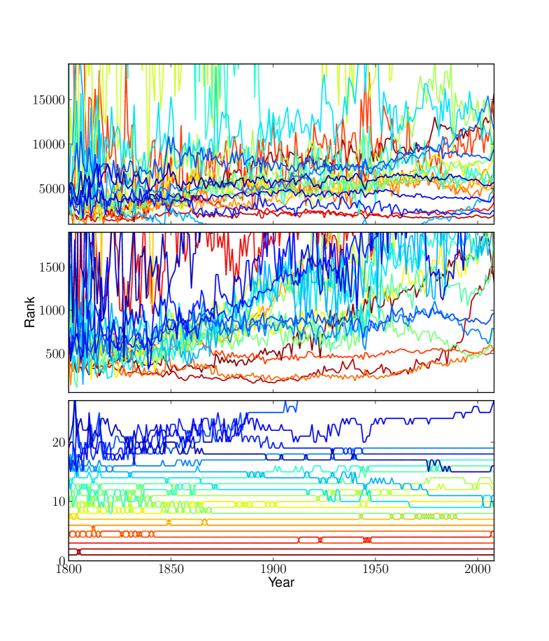
Figure 13: Rank variations in time of twenty words from three different scales for Italian.

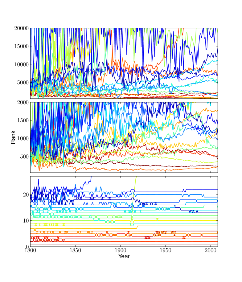
Figure 14: Rank variations in time of twenty words from three different scales for Spanish.

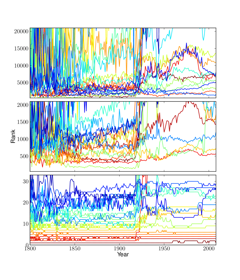
Figure 15: Rank variations in time of twenty words from three different scales for Russian.

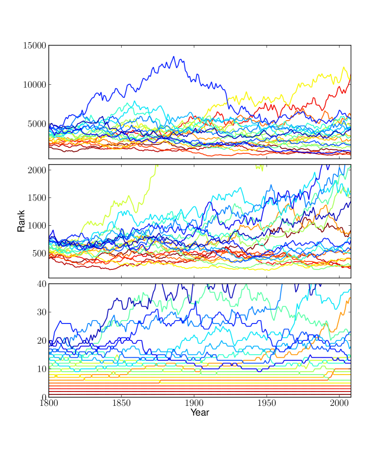
Figure 16: Rank variations in time of twenty words from three different scales for our simulated language.

Fig. 17 shows the distribution of relative flights for all languages. See main text for details.

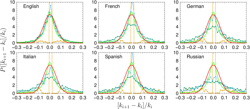
Figure 17: Distribution of relative flights for all languages studied. A similar plot as the one presented in figure 6 is shown for other languages. The same color coding and details are used.

S3 Correlation of relative frequency changes

We studied the correlations of the relative frequency changes (flights), defined in the main text as

$$\Delta_{t}=\left(k_{t+1}-k_{t}\right)/k_{t}.$$ (S22)

We shall use a normalized version of it:

$$d_{t}=\frac{\Delta_{t}-\langle\Delta_{t}\rangle}{\sqrt{\langle(\Delta_{t}-\langle\Delta_{t}\rangle)^{2}\rangle}},$$ (S23)

where $\langle\cdot\rangle$ denotes average over time. This normalization ensures that both $\langle d_{t}\rangle=0$ and $\langle d_{t}^{2}\rangle=1$. The time correlation is given by

$$C_{\tau}=\langle d_{t}d_{t+\tau}\rangle.$$ (S24)

In principle, this quantity also depends on $t$, but usually this dependence is very weak, as in this case, and one can ignore it.

In Fig. 18 we show the average of $C_{\tau}$, of 50 different ranks chosen randomly, for different languages, as well as for the simulated language. We note that the correlation is very small, except for $\tau=0$, where it is 1, due to the normalization chosen, and for $\tau=1$ where a negative value, typical of bounded sequences, is observed for the six languages studied here. The random Gaussian model reproduces well these correlations except at $\tau=1$.

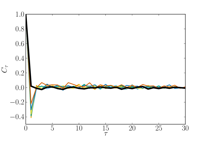
Figure 18: Correlations for relative frequency changes for different languages. Black line shows correlations for the simulated language.

References

- 1. Zipf GK (1932) Selective Studies and the Principle of Relative Frequency in Language. Cambridge, MA, USA: Harvard University Press.
- 2. Mandelbrot B (1953) An informational theory of the statistical structure of language. In: Jackson W, editor, Communication Theory, the Second London Symposium, London: Betterworth, chapter 36. pp. 486-502. URL http://www.uvm.edu/~pdodds/files/papers/others/1953/mandelbrot1953a.pdf.
- 3. Hawkins JA, Gell-Mann M, editors (1992) The Evolution of Human Languages: Proceedings of the Workshop on the Evolution of Human Languages, Held August, 1989 in Santa Fe, New Mexico. Perseus Books.
- 4. Ferrer i Cancho R, Solé RV (2002) Zipf’s law and random texts. Advances in Complex Systems 5: 1-6.
- 5. Baek SK, Bernhardsson S, Minnhagen P (2011) Zipf’s law unzipped. New Journal of Physics 13: 043004.
- 6. Corominas-Murtra B, Fortuny J, Solé RV (2011) Emergence of Zipf’s law in the evolution of communication. Phys Rev E 83: 036115.
- 7. Perc M (2012) Evolution of the most common English words and phrases over the centuries. Journal of The Royal Society Interface 9: 3323-3328.
- 8. Newman ME (2005) Power laws, Pareto distributions and Zipf’s law. Contemporary Physics 46: 323–351.
- 9. Clauset A, Shalizi CR, Newman ME (2009) Power-law distributions in empirical data. SIAM Review 51: 661–703.
- 10. Petruszewycz M (1973) L’histoire de la loi d’Estoup-Zipf: documents. Mathématiques et Sciences Humaines 44: 41–56.
- 11. Auerbach F (1913) Das gesetz der bevölkerungskonzentration. Petermanns Geographische Mitteilungen 59: 74–76.
- 12. Booth AD (1967) A ‘‘law’’ of occurrences for words of low frequency. Information and Control 10: 386–393.
- 13. Montemurro MA (2001) Beyond the Zipf–Mandelbrot law in quantitative linguistics. Physica A: Statistical Mechanics and its Applications 300: 567–578.
- 14. Font-Clos F, Boleda G, Corral A (2013) A scaling law beyond Zipf’s law and its relation to Heaps’ law. New Journal of Physics 15: 093033.
- 15. Gerlach M, Altmann EG (2013) Stochastic model for the vocabulary growth in natural languages. Phys Rev X 3: 021006.
- 16. Ferrer i Cancho R, Solé RV (2001) Two regimes in the frequency of words and the origins of complex lexicons: Zipf’s law revisited. Journal of Quantitative Linguistics 8: 165–173.
- 17. Bochkarev V, Solovyev V, Wichmann S (2014) Universals versus historical contingencies in lexical evolution. Journal of The Royal Society Interface 11: 20140841.
- 18. Takala S (1985) Estimating students’ vocabulary sizes in foreign language teaching. In: Practice and Problems in Language Testing, Afinla, volume 8. pp. 157–165. URL https://www.jyu.fi/hum/laitokset/solki/afinla/julkaisut/arkisto/40/takala.
- 19. Hall RA (1953) Haitian Creole: Grammar, Texts, Vocabulary. Philadelphia: American Folklore Society.
- 20. Romaine S (1988) Pidgin and Creole Languages. London: Longman.
- 21. Beare K (2014) Voice of America Special English Dictionary. About.com English as 2nd Language. URL http://esl.about.com/cs/reference/a/aavoa.htm.
- 22. Hornby AS (2005) Oxford Advanced Learner’s Dictionary. Oxford, UK: Oxford University Press. URL http://www.oxfordlearnersdictionaries.com/wordlist/english/oxford3000/ox3k_A-B/.
- 23. Michel JB, Shen YK, Aiden AP, Veres A, Gray MK, et al. (2011) Quantitative analysis of culture using millions of digitized books. Science 331: 176-182.
- 24. Wijaya DT, Yeniterzi R (2011) Understanding semantic change of words over centuries. In: Proceedings of the 2011 international workshop on DETecting and Exploiting Cultural diversiTy on the social web. ACM, pp. 35–40.
- 25. Serrà J, Corral Á, Boguñá M, Haro M, Arcos JL (2012) Measuring the evolution of contemporary western popular music. Scientific Reports 2: 521.
- 26. Petersen AM, Tenenbaum J, Havlin S, Stanley HE (2012) Statistical laws governing fluctuations in word use from word birth to word death. Scientific Reports 2: 313.
- 27. Blumm N, Ghoshal G, Forró Z, Schich M, Bianconi G, et al. (2012) Dynamics of ranking processes in complex systems. Physical Review Letters 109: 128701.
- 28. Acerbi A, Lampos V, Garnett P, Bentley RA (2013) The expression of emotions in 20th century books. PLoS ONE 8: e59030.
- 29. Perc M (2013) Self-organization of progress across the century of physics. Scientific Reports 3: 1720.
- 30. Febres G, Jaffe K, Gershenson C (2014) Complexity measurement of natural and artificial languages. Complexity Early View.
- 31. Hernández H (1988) Hacia un modelo de diccionario monolingüe del español para usuarios extranjeros. In: Actas del Primer Congreso Nacional de ASELE. pp. 159–166. URL http://cvc.cervantes.es/ensenanza/biblioteca_ele/asele/pdf/01/01_0307.pdf.
- 32. Steels L (1997) The synthetic modeling of language origins. Evolution of Communication 1: 1–34.
- 33. Chomsky N (1965) Aspects of the Theory of Syntax. Massachusetts Institute of Technology. M.I.T. Press. URL http://books.google.com.mx/books?id=u0ksbFqagU8C.
- 34. Hauser M, Chomsky N, Fitch W (2002) The faculty of language: What is it, who has it, and how did it evolve? Science 298: 1569.
- 35. Pinker S, Bloom P (1990) Natural language and natural selection. Behavioral and Brain Sciences 13: 707–727.
- 36. Kirby S (1999) Function, Selection, and Innateness: The Emergence of Language Universals. Oxford University Press.
- 37. Kirby S, Dowman M, Griffiths TL (2007) Innateness and culture in the evolution of language. Proceedings of the National Academy of Sciences 104: 5241-5245.
- 38. Chater N, Reali F, Christiansen MH (2009) Restrictions on biological adaptation in language evolution. Proceedings of the National Academy of Sciences 106: 1015-1020.
- 39. Nowak MA, Krakauer DC (1999) The evolution of language. Proceedings of the National Academy of Sciences 96: 8028-8033.
- 40. Steels L (1995) A self-organizing spatial vocabulary. Artificial Life 2: 319–332.
- 41. Sandler W, Meir I, Padden C, Aronoff M (2005) The emergence of grammar: Systematic structure in a new language. Proceedings of the National Academy of Sciences of the United States of America 102: 2661-2665.
- 42. Gell-Mann M, Ruhlen M (2011) The origin and evolution of word order. Proceedings of the National Academy of Sciences 108: 17290-17295.
- 43. Beuls K, Steels L (2013) Agent-Based Models of Strategies for the Emergence and Evolution of Grammatical Agreement. PLoS ONE 8: e58960+.
- 44. Brockmann D, Helbing D (2013) The hidden geometry of complex, network-driven contagion phenomena. Science 342: 1337-1342.
- 45. Ha LQ, Sicilia-Garcia EI, Ming J, Smith FJ (2002) Extension of Zipf’s law to words and phrases. In: Proceedings of the 19th International Conference on Computational Linguistics (COLING. pp. 315–320.
- 46. Batty M (2006) Rank clocks. Nature 444: 592–596.
- 47. Braha D, Bar-Yam Y (2006) From centrality to temporary fame: Dynamic centrality in complex networks. Complexity 12: 59–63.
- 48. Hausmann R, Hidalgo CA, Bustos S, Coscia M, Simoes A, et al. (2014) The Atlas of Economic Complexity: Mapping Paths to Prosperity. MIT Press.
- 49. Gross T, Sayama H, editors (2009) Adaptive networks: Theory, Models and Applications. Understanding Complex Systems. Berlin Heidelberg: Springer. doi:10.1007/978-3-642-01284-6. URL http://dx.doi.org/10.1007/978-3-642-01284-6.
- 50. Gautreau A, Barrat A, Barthélemy M (2009) Microdynamics in stationary complex networks. Proceedings of the National Academy of Sciences 106: 8847-8852.
- 51. Perra N, Gonçalves B, Pastor-Satorras R, Vespignani A (2012) Activity driven modeling of time varying networks. Scientific Reports 2: 469.
- 52. Holme P, Saramäki J (2012) Temporal networks. Physics Reports 519: 97–125.
- 53. Albert R, Barabási AL (2002) Statistical mechanics of complex networks. Rev Mod Phys 74: 47–97.
- 54. Jensen HJ (2008) Emergence of network structure in models of collective evolution and evolutionary dynamics. Proceedings of the Royal Society A: Mathematical, Physical and Engineering Science 464: 2207-2217.
- 55. McKane A, Alonso D, Solé RV (2000) Mean-field stochastic theory for species-rich assembled communities. Phys Rev E 62: 8466–8484.