Spin Amplification with Inhomogeneous Broadening

Abstract

A long-lived qubit is usually well-isolated from all other systems and the environments, and so is not easy to couple with measurement apparatus. It is sometimes difficult to implement reliable projective measurements on such a qubit. One potential solution is spin amplification with many ancillary qubits. Here, we propose a spin amplification technique, where the ancillary qubits state change depending on the state of the target qubit. The technique works even in the presence of inhomogeneous broadening. We show that fast and accurate amplification is possible even if the coupling and frequency of the ancillary qubits is inhomogeneous. Since our scheme is robust against realistic imperfections, this could provide a new mechanism for reading out a single spin that could not have been measured using the previous approaches.

Accurate quantum measurements and long coherence times are typical requirements for quantum information processing. It is essential to perform quantum measurements when we require quantum error correctioncorrection or need quantum feedback technology feedback .

Moreover, long coherence time is important in terms of retaining the quantum information during the waiting time for the next operations. A lot of progress has been made on the technique for fabricating a long-lived qubit with many physical systems, and the coherence time has been significantly improved. For example, an electron spin has a coherence time longer than a secondA.M.Tyryshkin , while the coherence time of a nuclear spin is longer than a minuteKamyar2013 . Even for an artificial two-level system such as a superconducting qubit, the coherence time is of the order of tens of microsecondsRigetti .

It is sometimes difficult to read out the signal from a long-lived qubit, because long-lived qubits do not generally couple well with the measurement apparatus. To increase the coherence time, the qubit should be isolated so that it has a tiny coupling strength with other external systems. On the other hand, to read out a qubit with high fidelity requires a strong coupling with the measurement apparatus, which may be contradicted by the fact that the qubit is isolated from other systems.

One solution for this problem is spin amplification. If we couple the target qubit to read out with many ancillary qubits, we can use the ancillary qubits to increase the effective signals, even if there is little individual coupling between the target qubit and ancillary qubits. If the target qubit is in the ground state, the ancillary qubits remain in the ground state, while the ancillary qubits will be excited if the target qubit is in the excited state. There has been a lot of researches in this direction. A simple quantum circuit, which consists of controlled-NOT gates, is a well-known example ganso ; ghz ; entanglement . However, in this scheme each spin must be independently accessible and interact with the target qubit and it is difficult to increase the scale of such a scheme. Although there have been some proposals as regards a scalable spin amplification, they require a special configuration for ancillary qubits with tailored couplingsC.A ; A.Kay ; J.A ; J.S and/or the protocol is fragile with respect to certain some imperfections such as the inhomogeneous broadening or thermal excitation of the ancillary qubitsClose2011 ; Negoro2011 .

In this paper, we suggest another way to amplify the signal of the target qubit where many ancillary qubits are collectively coupled with the target qubit. Since this is a simple experimental setup, there are many physical systems that have this configuration. A superconducting qubit coupled with a spin ensemble is one candidate for realizing our scheme Saitosan ; zhu ; Kubosanprl ; zhusan . A nuclear (or electron) spin coupled with many satellite nuclear (or electron) spins with different frequencies is another candidate Weimer .

In this paper, we address the problem of the inhomogeneous broadening in particularinhomo1 ; inhomo2 . In reality, it is very difficult to fabricate identical qubits so that every ancillary qubit can have a different frequency and also have a different coupling strength with the target qubit. Interestingly, in our scheme, we can realize rapid and reliable spin amplification even under the influence of inhomogeneous broadening. The target qubit is coupled with the collective mode of the ancillary qubits. On the other hand, the collective mode of the ancillary qubits is coupled with the subradiant modes of the qubits, which induces dissipation. If we try to realize coherence transfer between the target spin and the collective mode, the existence of the subradiant modes induces decoherence, which means the fidelity of the coherent transfer decreases. However, with spin amplification, coherence is not required because the purpose is to read out the target qubit, which eliminates the diagonal term of the density matrix of the target spin if the quantum measurement is successfully implemented. Moreover, we have shown that coupling between the collective mode and subradiant mode only induces an energy transfer from the former to the latter that can be also measured as well as the former. Our technique can provide a reliable readout of a qubit coupled with many inhomogeneous ancillary qubits.

The Hamiltonian of our hybrid system composed of the target qubit and ancillary qubits can be described by

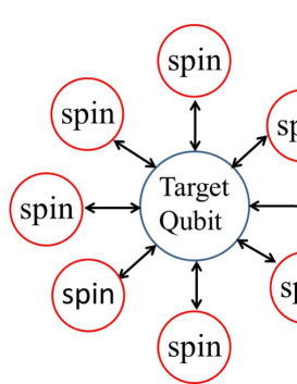
Figure 1: Schematic of our hybrid system. The central target qubit is collectively coupled with the ensemble of ancillary qubits. The target qubit can be readout via the ancillary qubits after the amprification technique

$$\hat{H}_{\text{TA}}= \frac{\omega_{T}}{2}\hat{\sigma}_{z}+\sum_{j=1}^{N}g_{j}(\hat{\sigma}^{-}\hat{\sigma}_{j}^{+}+\hat{\sigma}^{+}\hat{\sigma}_{j}^{-})+\sum_{j=1}^{N}\frac{\omega_{j}}{2}\hat{\sigma}_{zj}$$ (1)

$$+\lambda_{d}\mathrm{cos}(\omega_{d}t)(\hat{\sigma}^{+}+\hat{\sigma}^{-})$$

where we set $\hbar=1$. Here, $\hat{\sigma}_{z}$ denotes the Pauli z operator for the target qubit and $\hat{\sigma}^{-(+)}$denotes the ladder operator. $\omega_{T}$ and $\omega_{j}$ denote the resonant frequencies of the target qubit and the $j$ th spin, respectively. $\hat{\sigma}_{j}^{-(+)}$ and $\hat{\sigma}_{zj}$ denote the ladder operator and Pauli z operator of the $j$ th ancillary qubit, respectively. It is worth mentioning that, as long as most of the ancillary qubits are in the ground state and only a small portion of the ancillary qubits are excited for the amplification, we can consider the ancillary qubit to be a harmonic oscillator. So we can replace $\hat{\sigma}^{-(+)}_{j}$ with the annihilation(creation) operator $\hat{a}_{j}^{({\dagger})}$. $g_{j}$ is a real number and denotes the coupling strength between the target qubit and the $j$ th ancillary qubit. $\lambda_{d}$ denotes the Rabi frequency of the microwave applied to the target qubit. We assume that the coupling strength $g_{j}$ is much smaller than the inhomogeneous broadening width of this system. By employing a rotating frame defined by $\hat{U}(t)=\mathrm{exp}[-i\omega_{d}t(\frac{\hat{\sigma}_{z}}{2}+\sum_{j=1}^{N}\hat{a}_{j}^{\dagger}\hat{a}_{j})]$ and performing a rotating wave approximation, we have

$$\hat{H}_{RWA}\approx \frac{\omega_{T}-\omega_{d}}{2}\hat{\sigma}_{z}+\sum_{j=1}^{N}g_{j}(\hat{\sigma}^{-}\hat{a}_{j}^{\dagger}+\hat{\sigma}^{+}\hat{a}_{j})$$ (2)

$$+\sum_{j=1}^{N}(\omega_{j}-\omega_{d})\hat{a}_{j}^{\dagger}\hat{a}_{j}+\frac{\lambda_{d}}{2}(\hat{\sigma}^{+}+\hat{\sigma}^{-})$$

We will now model the effect of inhomogeneous broadening with a Lorentzian distribution of the resonant frequencies of the spin ensemble as

$$f(\omega)=\frac{1}{\pi}\frac{\gamma/2}{(\omega-\bar{\omega})^{2}+(\gamma/2)^{2}}$$ (3)

where, $\gamma$ denotes the width of the Lorentzian, and $\bar{\omega}$ denotes the average spin ensemble resonant frequency. We define the collective mode as follows

$$\hat{A}\equiv\frac{1}{G}\sum_{j=1}^{N}g_{j}\hat{a}_{j}$$ (4)

where $G=\sqrt{\sum_{j=1}^{N}g_{j}^{2}}$. Since we are mainly interested in the target qubit and collective mode, we can trace out the sub-radiant modes. In this case, the collective Hamiltonian can be written as Dinitz

$$\hat{H} =\hat{H}_{c}+\hat{H}_{d}\ \ \ \ \ \ \ \ \ \ \ \ \ \ \ \ \ \ \ \ \ \ \ \ \ \ \ \ \ \$$ (5)

$$\hat{H}_{c} =\frac{\omega_{T}-\omega_{d}}{2}\hat{\sigma}_{z}+G(\hat{A}\hat{\sigma}^{+}+\hat{A}^{\dagger}\hat{\sigma}^{-})+(\bar{\omega}-\omega_{d})\hat{A}^{\dagger}\hat{A}$$ (6)

$$\hat{H}_{d} =\frac{\lambda_{d}}{2}(\hat{\sigma}^{+}+\hat{\sigma}^{-})\ \ \ \ \ \ \ \ \ \ \ \ \ \ \ \ \ \ \ \ \ \ \ \ \ \ \ \ \$$ (7)

The width of the Lorentzian $\gamma$ can be incorporated in the dynamics as the decay term of the master equation, which we will discuss later.

In our scheme, we will drive the target qubit with a microwave pulse for the spin amplification. The collective mode coupled with the target qubit may differ from the collective mode coupled with the microwave line, which is called a mode mismatchmismatch . This problem means that driving the collective mode by the coupling between the microwave line and ancillary qubits is not straightforward. On the other hand, as we explain later, it is possible to drive the collective mode of the ancillary qubits by driving the target qubit. We have developed an efficient technique for calculating the number of excitations in the spin ensemble after driving. If we include the all freedom of N ancillary qubits, we need to deal with $2^{N+1}$ sized matrix, which is intractable. On the other hand, with the technique that we propose here, we need to solve a Hamiltonian that includes a single qubit and a harmonic oscillator, which is much easier to simulate. Using Eq.Spin Amplification with Inhomogeneous Broadening as a basis, we can write the Heisenberg equation,

$$\frac{d}{dt}\hat{a}(t)_{j}=-ig_{j}\hat{\sigma}(t)^{-}-i(\omega_{j}-\omega_{d}-i\frac{\Gamma}{2})\hat{a}(t)_{j}$$ (8)

where we add the energy decay term $\Gamma$ of the ancillary qubit. However, this decay rate is usually negligible compared with that of other noise. For example, the energy relaxation time of an electron such as the NV^- center exceeds 200 seconds inhomo4 . So we adopt a limit of $\Gamma\rightarrow 0$, later. Now

$$\frac{d}{dt}\sum_{j=1}^{N}\hat{a}(t)_{j}^{\dagger}\hat{a}_{j}=iG(\hat{\sigma}^{+}\hat{A}(t)-\hat{A}(t)^{\dagger}\hat{\sigma}^{-})-\Gamma\sum_{j=1}^{N}\hat{a}(t)_{j}^{\dagger}\hat{a}(t)_{j}$$ (9)

Now, taking the Laplace transforms of both sides of Eq.8, under the initial conditions $a_{j}(0)=0,\sigma^{-}(0)=0$, we have

$$\hat{\alpha}_{j}(s)=-\frac{ig_{j}\hat{\beta}(s)}{s+i(\omega_{j}-\omega_{d}-i\frac{\Gamma_{s}}{2})}$$ (10)

Here, $\hat{\alpha}_{j}(s)=\mathcal{L}[\hat{a}_{j}(t)],\hat{\beta}(s)=\mathcal{L}[\hat{\sigma}^{-}(t)].$ Using the Lorentzian distribution (3) and adopting residual integration, we obtain

$$\frac{1}{G}\sum_{j=1}^{N}g_{j}\hat{\alpha}_{j}(s)=-\frac{iG\hat{\beta}(s)}{s+i(\bar{\omega}-\omega_{d}-i\frac{\gamma+\Gamma}{2})}$$ (11)

Taking the inverse Laplace transformation of both sides, we obtain

$$iG\sigma^{-}(t)=-\frac{d}{dt}\hat{A}(t)-i(\overline{\omega}-\omega_{d}-i\frac{\gamma+\Gamma_{s}}{2})\hat{A}(t)$$ (12)

By using Eq.12 and Eq.9, in the limit of $\gamma>>\Gamma$ we obtain

$$\frac{d}{dt}(-\hat{A}^{\dagger}(t)\hat{A}(t)+\sum_{j=1}^{N}\hat{a}_{j}^{\dagger}(t)\hat{a}(t)_{j})=\gamma\hat{A}^{\dagger}(t)\hat{A}(t)$$ (13)

This means that the rate of increase of the subradiant modes ($-\hat{A}^{\dagger}(t)\hat{A}(t)+\sum_{j=1}^{N}\hat{a}_{j}^{\dagger}(t)\hat{a}_{j}(t)$) depends on the collective mode ($\hat{A}^{\dagger}(t)\hat{A}(t)$) and the inhomogeneous width ($\gamma$). By integrating Eq.13, we obtain

$$\sum_{j=1}^{N}\hat{a}(t)_{j}^{\dagger}\hat{a}(t)_{j}=\hat{A}(t)^{\dagger}\hat{A}(t)+\gamma\int_{0}^{t}\hat{A}(t^{\prime})^{\dagger}\hat{A}(t^{\prime})dt^{\prime}$$ (14)

By calculating he dynamics of A(t), we can estimate the excitation number $\sum_{j=1}^{N}\hat{a}_{j}(t)^{\dagger}\hat{a}_{j}(t)$

We intuitively explain how our amplification works. If the detuning between the energy of the target qubit and the frequency of the collective mode is much larger than the coupling strength, we can derive the dispersive Hamiltonian as follows intro .

$$\hat{H}_{disp}=\frac{\omega_{T}-\omega_{d}}{2}\hat{\sigma}_{z}+\frac{G^{2}}{\Delta}\hat{\sigma}^{+}\hat{\sigma}^{-}+(\bar{\omega}-\omega_{d}+\frac{G^{2}}{\Delta}\hat{\sigma}_{z})\hat{A}^{\dagger}\hat{A}$$ (15)

where $\lambda_{d}=0$ and $\Delta=(\omega_{T}-\omega_{d})-(\bar{\omega}-\omega_{d})$. This means that, depending on the state of the target qubit, there is a dispersive energy shift as follows.

$$\bar{\omega}\Rightarrow\bar{\omega}\pm\frac{G^{2}}{\Delta}$$ (16)

So, if the driving frequency is $\bar{\omega}+\frac{G^{2}}{\Delta}$ and the target qubit is in an excited state, the ensemble of the ancillary qubits is efficiently excited. On the other hand, if the driving frequency is $\bar{\omega}+\frac{G^{2}}{\Delta}$ and the target qubit is in the ground state, the spin ensemble is not significantly affected by the driving caused by the detuning. Throughout this paper, we fix the driving frequency as $\bar{\omega}+\frac{G^{2}}{\Delta}$.

Although we later solve the master equation numerically, it is also possible to describe the dynamics of the collective mode in an analytical way by using an approximation. By diagonalizing the $H_{c}$ in Eq.6, we obtainintro

$$\hat{H}_{c}=\sum_{n}\hat{H}_{n}$$ (17)

$$\hat{H}_{n}=\Omega_{+}(n)\ket{+,n}\bra{+,n}+\Omega_{-}(n)\ket{-,n}\bra{-,n}$$ (18)

$$\Omega_{\pm}(n)=(n+\frac{1}{2})(\bar{\omega}-\omega_{d})\pm\frac{\sqrt{\Delta^{2}+4G^{2}(n+1)}}{2}$$ (19)

The eigenstate of the Hamiltonian is

$$\ket{+,n}=\mathrm{cos}(\phi_{n}/2)\ket{e,n}+\mathrm{sin}(\phi_{n}/2)\ket{g,n+1}$$ (21)

$$\ket{-,n}=-\mathrm{sin}(\phi_{n}/2)\ket{e,n}+\mathrm{cos}(\phi_{n}/2)\ket{g,n+1}$$ (22)

$$\phi_{n}=\mathrm{tan}^{-1}\bigg{(}\frac{2G\sqrt{n+1}}{\Delta}\bigg{)}$$ (23)

where $|e\rangle$ ($|g\rangle$) denotes the excited (ground) state of the target qubit and $|n\rangle$ denotes the number state of the collective mode. Since we can diagonalize the Hamiltonian $H_{c}$, we can efficiently use an interaction picture where we define $\hat{U}=e^{-iH_{c}t}$ and $H_{I}(t)=\hat{U}^{\dagger}\hat{H}_{d}\hat{U}$. By using the condtion $\Delta\gg G$, we obtain

$$H_{I}(t)\simeq\lambda_{eff}\Big{(}|e\rangle\langle e|(\hat{A}+\hat{A^{\dagger}})-|g\rangle\langle g|(\hat{A}e^{i\frac{2G^{2}}{\Delta}t}+\hat{A^{\dagger}}e^{-i\frac{2G^{2}}{\Delta}t})\Big{)}$$ (24)

where $\lambda_{eff}=\frac{\lambda_{d}}{2}\frac{G}{\Delta}$ denotes the effective Rabi frequency of the collective mode. If the initial state of the target qubit is $|e\rangle$ and it remains unchanged during the time evolution, we can derive the Hamiltonian for the collective mode $H^{(\text{anc})}_{I}(t)\simeq\lambda_{eff}(\hat{A}+\hat{A^{\dagger}})$. On the other hand, if the target qubit is kept in the ground state, we obtain $H_{I}(t)\simeq-\lambda_{eff}(\hat{A}e^{i\frac{2G^{2}}{\Delta}t}+\hat{A^{\dagger}}e^{-i\frac{2G^{2}}{\Delta}t})$. By returning to the Schrodinger picture, we obtain

$$\hat{H}_{anc}=(\bar{\omega}-\omega_{d}\pm\frac{G^{2}}{\Delta})\hat{A}^{\dagger}\hat{A}\pm\lambda_{eff}(\hat{A}+\hat{A}^{\dagger})$$ (25)

where the sign $\pm$ depends on the state of the target qubit. With this Hamiltonian, we obtain the Heisenberg equation of $\hat{A}$ as follows,

$$\frac{d}{dt}\hat{A}=-i(\bar{\omega}-\omega_{d}\pm\frac{G^{2}}{\Delta}-i\frac{\gamma}{2})\hat{A}-i\lambda_{eff}$$ (26)

where we added the energy relaxation term $-i\frac{\gamma}{2}\hat{A}$. When the target qubit is in an excited state, we solve this equation analytically with $\omega_{d}=\bar{\omega}+\frac{G^{2}}{\Delta}$, and obtain

$$\braket{\hat{A}^{\dagger}(t)\hat{A}(t)}=\frac{4\lambda_{eff}^{2}}{\gamma^{2}}\bigg{(}1-e^{-\frac{\gamma}{2}t})^{2}$$ (27)

On the other hand, when the target spin is in the ground state, we obtain

$$\braket{\hat{A}^{\dagger}(t)\hat{A}(t)}=\frac{\lambda_{eff}^{2}}{(\frac{2G^{2}}{\Delta})^{2}+(\frac{\gamma}{2})^{2}}\bigg{[}1-2\mathrm{cos}\bigg{(}\frac{2G^{2}}{\Delta}t\bigg{)}e^{-\frac{\gamma}{2}t}+e^{-\gamma t}\bigg{]}$$ (28)

It should be noted that, if the effective Rabi frequency is far smaller than the dispersive energy shift such as $\lambda_{eff}\ll\frac{G^{2}}{\Delta}$, the excitation of the collective mode is significantly suppressed when the target qubit is prepared in the ground state. So we retain this condition throughout this paper.

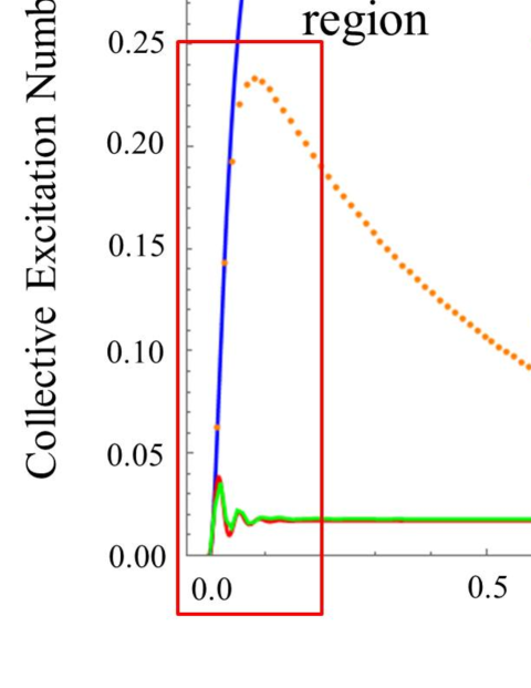
Figure 2: Collective mode excitation number against time. Solid lines show analytical solutions and dashed lines show numerical calculations where we set $\gamma/2\pi=12.5$ MHz, $G/2\pi$=75 MHz, $\Delta/2\pi=412.5$ MHz, and $\lambda_{d}/2\pi=40$ MHz. These are typical parameters of the hybrid system composed of superconducting flux qubit and NV- centerszhu . When obtaining analytical solutions, we use a dispersive Hamiltonian where the state of the target qubit is not changed, which is a valid approximation for a short time region (dispersive region). However, for a numerical simulation, the excited state of the target qubit decays into the ground state due to the flip flop term of the JC Hamiltonian and subradient mode, which leads a difference from the analytical approach for a longer time scale.

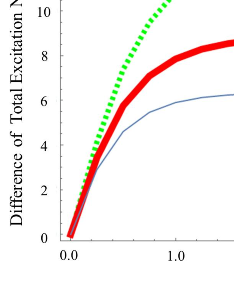
Figure 3: Spin amplification process in our scheme. Depending on the initial state of the target qubit ($|e\rangle$ or $|g\rangle$), the ancillary qubit excitations numbers differ, and we plot this difference against time. We set the parameters at $G/2\pi=75$ MHz, $\lambda_{d}/2\pi=40$ MHz, $\Delta/2\pi=412.5$ MHz

We calculate the time evolution of the collective mode by solving the following master equation.

$$\frac{d\hat{\rho}}{dt}=-i[\hat{H},\hat{\rho}]+\frac{\gamma}{2}[2\hat{A}\hat{\rho}\hat{A}^{\dagger}-\hat{A}^{\dagger}\hat{A}\hat{\rho}-\hat{\rho}\hat{A}^{\dagger}\hat{A}]$$ (29)

It is worth mentioning that the inhomogeneous broadening of the frequency can be considered an energy loss of the collective mode Dinitz . In Fig.2, we plot the time evolution of the collective mode by using the analytical approach described above and a numerical approach to solve the master equation of Eq. 29. We assume that the initial state is $|e,0\rangle$ or $|g,0\rangle$. In the analytical approach, the state of the target spin does not change during the time evolution, because we use a dispersive Hamiltonian. When the initial state of the target qubit is an excited state, the collective mode of the spin ensemble is excited efficiently in both the numerical simulation and the analytical calculation for a short time scale. However, since the energy of the target qubit is gradually transfered to the subradiant modes of the ancillary qubits, the target qubit decays into the ground state and so the collective mode will not be efficiently excited over a long time period in the numerical simulation enhanced . This induces a disagreement between the analytical solution and numerical simulation in this regime. On the other hand, when the initial state of the target qubit is the ground state, the state of the target will not be significantly changed, and so there is an excellent agreement between all $t$ values of the analytical solution and numerical simulation where the excitation of the collective modes is efficiently suppressed.

We plot the difference in the excitation population of the ensemble when the target qubit is in its excited and ground states in Fig.3. Although the inhomogeneous broadening reduces the efficiency of the amplification, we can still obtain a difference of more than 10 excitations in the ancillary qubits for $\gamma/2\pi=10$ MHz. This means that we will have a 10 times better signal with our amplification technique than without any amplification, which would provide us with a practical tool with which to read out a single qubit such as an electron spin or a nuclear spin.

In conclusion, we have proposed a spin amplification technique that can be used in the presence of the inhomogeneous broadening. We considered a simple experimental system where a target qubit is collectively coupled with many ancillary qubits. We showed that, even if the ancillary qubits are inhomogeneous, we can amplify the signal from the target spin, and obtain a gain of 10 in such a system by applying a continuous microwave. Our technique opens the way to the fast and robust readout of a single spin.

We thank H. Yamaguchi and J. Hayase for valuable discussions. We thank T. Koike for encouraging S. Endo’s research. This work was supported by Commissioned Research No. 158286 of National Institute of Information and Communication 287 Technology (NICT).

References

- (1) D.A. Linder et al., ”Quantum error correction.” Cambridge University Press, 2013.
- (2) W. M. Howard et al., ”Quantum measurement and control.” Cambridge University Press, 2009.
- (3) A.M. Tyryshkin et al., Nature Materials 11, 143-147 (2011).
- (4) K. Saeedi et al., Science 342, 830 (2013).
- (5) C. Rigetti et al., Phys. Rev. B 86, 100506 (2012).
- (6) D. P. DiVincenzo, et al., Phys. 48, 771 (2000).
- (7) P. Cappellaro et al., Phys. Rev. Lett. 94, 020502 (2005).
- (8) J. A. Jones et al., Science 324, 1166 (2009).
- (9) C. A. Peŕez-Delgado et al., Phys. Rev. Lett. 97, 100501 (2006).
- (10) A. Kay, Phys. Rev. Lett. 98, 010501 (2007).
- (11) J. A. Jones et al., Science 324, 1166 (2009).
- (12) J. S. Lee et al., New J. Phys. 9, 83 (2007).
- (13) T. Close et al., Phys. Rev. Lett. 106, 167204 (2011).
- (14) M. Negoro et al., Phys. Rev. Lett. 107, 050503 (2011).
- (15) S. Saito et al., Phys. Rev. Lett. 111, 107008 (2013).
- (16) X. Zhu et al., Nature 478, 221 (2011).
- (17) Y. Kubo et al., Phys. Rev. Lett. 107, 220501 (2011).
- (18) X. Zhu et al., Nat. Commun. 5, 3424 (2014).
- (19) H. Weimer et al., Phys. Rev. Lett. 110, 067601 (2013).
- (20) B. Kraus et al., Phys. Rev. A 73, 020302 (2006).
- (21) J. H. Wesenberg, et al., Phys. Rev. Lett. 103, 070502 (2009) .
- (22) I. Diniz et al., Phys. Rev. A 84, 063810 (2011).
- (23) J. Wei et al., Phys. Rev. A 69, 043819 (2004).
- (24) R. Amss et al., Phys. Rev. Lett. 107, 060502 (2011).
- (25) C.C. Gerry et al., ”Introductory Quantum Optics” Cambridge University Press, 2004.
- (26) Y. Matsuzaki et al., Phys. Rev. B 86, 184501 (2012).