Spontaneous second order phase transition. Amorphous branch

Abstract

A version of the second order phase transition theory, in which the Nernst theorem holds automatically, is proposed. The theory is constructed in terms of the order parameter and the (configurational) entropy. It faithfully reproduces the solutions of Landau theory as well as stable existence of ordered and disordered states and takes into account the existence of amorphous metastable states. Finally, phenomenon of growth of fluctuations magnitude due to random first order transitions between stable and metastable states as their energies approach each other at a critical point is analyzed.

The Landau theory of the second order phase transitions (PT-2) was proposed in the middle of previous century Landau-1 (1937), but interest to it still persists. The theory is widely applied for study of phase transitions in structural, magnetic, liquid crystal and incommensurate systems Toledano et al. (1985); J.C.Toledano and P.Toledano (1987); Toledano (1994, 2012), for study of re-orientational phase transitions Belov et al. (1976); Tsymbal et al. (2005). It had been substantially developed by modern phase fields theories Aranson et al. (2000); Eastgate et al. (2002); Rosam et al. (2009); Choudhury et al. (2012). It is also used in studies of polymorph transformations of liquid – liquid type in molten silicon between liquid phases with differ density McMillan et al. (2007). A great many variants of PT-2 theory was developed in the context of amorphous material problems, for example Adam et al. (1965); Gibbs et al. (1958); Tanaka at all (2010); Krasnuk at all (2012). At the same time, it is known that this theory is not suitable to the description of amorphous meta-stable states Kirkpatrick et al. (2014). This is because amorphous states correspond to the maxima of thermodynamic potential, and therefore they are not absolutely stable. To modify this theory to be to describe amorphous meta-stable states, we will now reconsider several foundational aspects of this theory.

It is well known that PT-2 theory does not satisfy the Nernst theorem. It follows from the connection between order parameter (OP) $\varphi$ and entropy $s$ Patashinsky and Pokrovsky (1979)

$$s=-\frac{\partial f}{\partial T}=-\frac{\alpha}{2T_{c}}\varphi^{2}.$$ (1)

where $f$ is the free energy, $T$ is the temperature, $\alpha$ is a positive constant, $T_{c}$ is the critical temperature.

From here we notice that the entropy is negative for real OP ($\varphi^{2}>0$), that is in ordering region. To satisfy the Nernst theorem one can choose the free energy in the form

$$f=f_{0}-T\frac{\alpha^{2}}{2bT_{c}}+\frac{1}{2}\alpha\frac{T-T_{c}}{T_{c}}\varphi^{2}+\frac{1}{4}b\varphi^{4}.$$ (2)

where $b$ is another constant.

It differs from the standard PT-2 theory only by the fact that the free term has a specific temperature dependence. Notice that equilibrium meaning of the OP in this case remains the same as in the reference theory,

$$\varphi_{0}=0,\quad\varphi_{1,2}=\pm(\dfrac{\alpha}{b}\dfrac{T_{c}-T}{T_{c}})^{1/2}.$$ (3)

But the connection (1) between the OP and the entropy in this case is now different (see variant Metlov (2013))

$$s=-\frac{\partial f}{\partial T}=\frac{\alpha}{2T_{c}}(\frac{\alpha}{b}-\varphi^{2}),$$ (4)

so that the entropy becomes a positive quantity inside the ordering interval and zero at zero temperature.

One-to-one connection (4) means that it is possible to choose either OP $\varphi$ or configuration entropy $s$, as an independent thermodynamics variable, and to express the PT-2, for example, not in terms of OP, but in terms of the configurational entropy. Performing the change of variables inside this interval, we obtain

$$f=f_{0}^{*}-Ts+b(\frac{T_{c}}{\alpha})^{2}s^{2}.$$ (5)

All is simple and with taste. Here $f_{0}^{*}=f_{0}-\alpha^{2}/4b$.

An equilibrium value of the entropy in this representation

$$s_{1}=\frac{\alpha^{2}}{2bT_{c}^{2}}T$$ (6)

after taking in account the connection (4) coincides by its absolute value with equilibrium values $\varphi_{1,2}$ (3) of the classical theory. Here the coefficient $K$ plays the role of the temperature sensitivity.

Note, that the density of the internal energy in this case takes an especially simple form

$$T=f-Ts=f_{0}^{*}+b(\frac{T_{c}}{\alpha})^{2}s^{2}$$ (7)

with maximum at $s=0$, aand with no explicit temperature dependence (in equilibrium the implicit temperature dependence of the internal energy is via $s_{1}$). The expression for equilibrium (thermostat) temperature is given by the classic formula

$$u=\frac{du}{dT}=2b(\frac{T_{c}}{\alpha})^{2}$$ (8)

which is identical to (6).

In accordance to (6) the equilibrium configurational entropy is zero at $T=0$, grows linearly with temperature and arrives to the maximal value (saturation) at the critical point $T=T_{c}$ (straight line 1, fig. 1). Thus the equilibrium states $\varphi_{1,2}$ in the form (3) by virtue of quadratic connection (4) merge together in one state in the form (6), and the stable equilibrium state $\varphi_{0}$ in the interval $T>T_{c}$ disappears from a consideration at all.

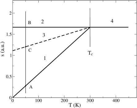
Figure 1: . Temperature diagram of the entropy of equilibrium and metastable states: the line 1 corresponds to the ordered state, 2 to the amorphous state, 3 to the line of maxima of free energy, 4 to the disordered state.

Therefore, we propose the new free energy expression to describe the equilibrium stable states on the interval $T>T_{c}$

$$f=f_{0}^{*}+\frac{\alpha^{2}}{2b}-T\frac{\alpha^{2}}{2bT_{c}}-T_{c}s+b(\frac{T_{c}}{\alpha})^{2}s^{2}.$$ (9)

satisfies all the necessary requirements, namely the equilibrium entropy $s_{2}$ remains at a constant maximum on the interval $T>T_{c}$

$$s_{2}=\frac{\alpha^{2}}{2bT_{c}}=s_{max}.$$ (10)

which corresponds to a zero equilibrium in (3). The expression (10) coincides with the expression (6) at the point $T=T_{c}$. Also, the temperature derivative of the free energy, taken with the minus sign, coincides identically with the entropy at this point.

Thus, consideration in terms of the entropy turns out somewhat more difficult (it makes it necessary to determine the free energies on different temperature intervals independently). It would only be the question of comfort, but let us consider the reverse transition. Using the connection (4), let us express the free energy (9) again in terms of the order parameter

$$f=f_{0}-T\frac{\alpha^{2}}{2bT_{c}}+\frac{1}{4}b\varphi^{4},$$ (11)

which does not coincide (due to the missing quadratic term) with the general expression (2). which must be valid on the whole temperature interval. Thus, the choice of variables is not the question of comfort, but of the correctness of the theory, at least, in the interval $T>T_{c}$.

Lett us show that the new form of the free energy (9) is physically more meaningful. At first, solution in the form (9), in the temperature interval $T>T_{c}$ can be continued to the region $T<T_{c}$. Indeed, there are no prohibitions on its existence in this area. But it turns out then, that in the area $T<T_{c}$ simultaneously exist not one (the sign of the order parameter is not taken into account), but two stable states, one of which is well-ordered (straight line 1, fig. 1), and the second contains the frozen-in disorder or amorphous state (straight line 2, fig. 1), which was not present in the standard theory. The minimum of the free energy for well-ordered states (curve 1, fig. 2) is deeper than the minimum for the amorphous state (straight line 2, fig. 2), and therefore it is the main state of the system. The amorphous state is meta-stable or “excited”state.

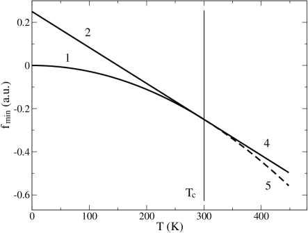
Figure 2: Temperature dependence of the free energy at the minima: 1 corresponds to the ordered state, 2 to the amorphous state, 3 to the maxima of free energy, 4 to the disordered state, 5 is unphysical continuation of the ordered states.

Note that a formal extension of the free energy in the form (5) to the area $T>T_{c}$ in accordance with (6) leads to the unlimited entropy growth, and, consequently, in accordance to (4) to the imaginary values of OP, which is non-physical. In accordance to our concepts the system arrives at the maximum disorder along this degree of freedom and its further increase over this degree of freedom becomes impossible.

So, on a temperature interval below than critical point the two stable equilibrium states $s_{1}$ and $s_{2}$ are possible. There is a problem, how to distinguish between them, where the line of a maximum of the free energy passes, and what is the height of the potential barrier between these states. This issue needs additional model assumptions. Let us consider that the «watershed» line between the stable states (lines 1 and 2, fig. 1, 2) is a straight line (dotted line 3, fig. 1). It goes from a critical point under a smaller angle, than the line for the well-ordered state (line 1, fig. 1). We set an equation of this line in a form

$$s_{3}=s_{max}^{(0)}+(s_{max}-s_{max}^{(0)})\frac{T}{T_{c}}.$$ (12)

Here the parameter $s_{max}^{(0)}$ determines the width of area of ordering, along the line 1 (fig. 1).

We can restore the profile of the free energy in a power approximation from elements of the model using the equations for equilibrium states

$$f=A\int(s-s_{1})(s-s_{2})(s-s_{3})ds.$$ (13)

The free energy curves at different values of the parameter $s_{max}^{(0)}$ are shown in fig. 3. For convenience of the comparison to the standard theory, the graphics is plotted in the OP representation by making use of the relation (4). One can see that positions of equilibrium states $\varphi_{1}$ and $\varphi_{2}$ strictly coincide in both models. At the same time, in the region of zero OP the standard theory predicts unstable state of the system (maximum of the free energy), while in our case the system in this region is meta-stable and, in the absence of large fluctuations at low temperatures, it can exist in such a state for unlimited time. Notice that the minimum of the free energy in this region is quite gentle and the system states are in an indifferent equilibrium position in a wide region of OP values. This marks the possibility of realization of large number of amorphous structure variants, such as those with fractal landscapes of the free energy Charbonneau at all (2014) that pre-determines a super-slow dynamics of system evolution into this region between amorphous states.

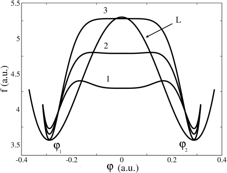
Figure 3: The dependence of the free energy on the order parameter at the temperature $T=50K$. The curve 1 is for $s_{max0}=s_{max}/1.5$, the curve 2 is for $s_{max0}=s_{max}/1.2$, the curve 3 is for $s_{max0}=s_{max}$ in our free energy expression, the curve $L$ corresponds the standard theory.

It is interesting to investigation the passage of the critical point by a system at heating or cooling from the positions of proposed theory. For example, at cooling near the critical point $T_{c}$ the system can go to the branch 1 (ground-state) or to the branch 2 (excited or amorphous state). Due to thermal fluctuations near the critical point the system will chaotically jump between these states. The probability of jumping into the ground-state is higher, that’s why it is realized at slow cooling (fig. 4, a). However, at fast cooling or at the narrow enough area of ordered states (small $s_{max}^{(0)}$) the system can remain in the chaotic state (quenching, fig. 4, b).

Thus, for the ordered states (lines 1) the chaotic states (lines 2) can be considered, as structural fluctuations between the chaotic states the ordered states. As fluctuations appear in the area of attraction of the proper nearest minimum, they will be long-living. Exactly, these long-living fluctuations determine the nature of growth of fluctuations near the critical point (opalescence, region 3, fig. 4).

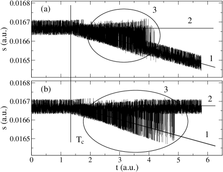
Figure 4: Generation of long-living fluctuations at passing of critical point by the drop in the temperature in the case of the ordered state formation (a) and in the case of the amorphous state formation (b). 1 is the line of the ordered states, 2 is the line of the amorphous states, 3 is the region of fluctuations growth

To simulate this process consider the evolution equation of Landau-Khalatnikov in the entropy representation

$$\frac{\partial s}{\partial t}=-\gamma_{s}((T-T_{c})\Theta(T-T_{c})-T+2b(\frac{T_{c}}{\alpha})^{2}s+Tf(s)).$$ (14)

where $\Theta(x)$ is theta-function, entered for comfort, $Tf(s)$ is a random function such as “white noise”, which is proportional to the temperature to simulate the thermal fluctuations.

The rest of the parameters were $\alpha=1$, $b=0.1$, $T_{c}=300K$. The initial temperature of thermostat was taken at $T=301K$, which is a little higher than critical, and goes down slowly.

In the vicinity of the critical temperature, predictably, there are severe long-living fluctuations. Each such fluctuation is connected with penetration of the potential barrier between the main and the meta-stable states, that it is the first order phase transition. As long as barrier is high enough in the low temperature region the fluctuations are absent. When the energy levels of the main and the meta-stable states approach each other and the potential barrier is reduced, the magnitude of thermal fluctuation becomes high enough to overcome it, which gives rise to the formation of severe (structural) fluctuations. This phenomenon is similar to phenomena of the random first order phase transitions in amorphous materials Kirkpatrick et al. (1989).

It is interesting that in at the critical point itself the long-living fluctuations do not form, and the general level of fluctuations does not exceed the thermal background. It is related to the fat that distinction between the two types of steady-states is vanishing at the critical point, and they can not “trap”the thermal fluctuations for each other. The growth of fluctuations, therefore, takes place not strictly at a critical point, but a little bit away from it to the side of the disordered states.

The level of fluctuations linearly increases with the distance from a critical point (due to the increase of the energy difference between the levels), but frequency of fluctuation diminishes. Finally, intensive structural fluctuations are halted, and the system gets trapped into one of the stable states. At slow cooling it always arrives into the main well-ordered state (branch 1, fig. 1), at fast cooling it can be trapped into the meta-stable amorphous state.

Thus, in this article the second order phase transitions theory is formulated in terms of the entropy (configuration or structural). It reproduces, as limiting cases, all the steady-states and transitions of the standard theory, but also reveals new solutions, which were missing from the classic theory. It allows to consider the processes of super-cooling or quenching naturally. The new mechanism of fluctuations growth at the critical temperature is based on the closeness of the two stable states. Its important feature is that the maximum of fluctuations growth is not exactly at the critical point, but is displaced from it.

References

- Landau-1 (1937) L. D. Landau, Phys. Z. Sowjetunion 11, 26 (1937).
- Toledano et al. (1985) P. Toledano, H. Schmid, M. Clin, and J. P. Rivera, Phys. Rev. B 32, 6006 (1985).
- J.C.Toledano and P.Toledano (1987) J. C. Toledano and P. Toledano, The Landau Theory of Phase Transitions: Application to Structural, Incommensurate, Magnetic and Liquid Crystal Systems (World Scientific, Singapore, 1987).
- Toledano (1994) P. Toledano, Ferroelectrics 162, 257 (1994).
- Toledano (2012) P. Toledano, EPJ Web of Conferences 22, 00007 (2012).
- Belov et al. (1976) K. P. Belov, A. K. Zvezdin, A. M. Kadomtseva, and R. Z. Levitin, Sov. Phys. Usp. (Sov. Adv. Phys.) 16, 574 (1976).
- Tsymbal et al. (2005) L. T. Tsymbal, Ya. B. Bazalii, G. N. Kakazei, Yu. I. Nepochatykh, and P. E. Wigen, Low Temperature Physics 31, 227 (2005).
- Aranson et al. (2000) I. S. Aranson, V. A. Kalatsky, and V. M. Vinokur, Phys. Rev. Lett. 85, 118 (2000).
- Eastgate et al. (2002) L. O. Eastgate, J. P. Sethna, M. Rauscher, T. Cretegny, C. S. Chen, and C. R. Myers, Phys. Rev. E 65, 036117 (2002).
- Rosam et al. (2009) J. Rosam, P. K. Jimack, and A. M. Mullis, Phys. Rev. E 79, 030601(R) (2009).
- Choudhury et al. (2012) A. Choudhury, and B. Nestler, Phys. Rev. E 85, 021602(16) (2012).
- McMillan et al. (2007) P. F. McMillan, M. Wilson, M. C. Wilding, D. Daisenberger, M. Mezouar, and G. N. Greaves, J. Phys.: Cond. Matter 19, 415101(41) (2007).
- Adam et al. (1965) A. Adam and J. Gibbs, J. Chem. Phys. 43, 139 (1965).
- Gibbs et al. (1958) J. Gibbs and E. Dimarzio, J. Chem. Phys. 28, 373 (1958).
- Tanaka at all (2010) H. Tanaka, T. Kawasaki, H. Shintani, and K. Watanabe, Nat.Mater. 9, 324 (2010).
- Krasnuk at all (2012) I. B. Krasnuk, T. N. Melnik, and V. M. Yurchenko, Scientific records of Tavriya national university 25(64), 1, 193 (2012).
- Kirkpatrick et al. (2014) T. R. Kirkpatrick and D. Thirumalai, eprint arXiv:1401.2024v1.
- Patashinsky and Pokrovsky (1979) A. Z. Patashinsky and V. L. Pokrovsky, Fluctuation Theory of Phase Transitions (Pergamon Press, Oxford, 1979).
- Metlov (2013) L. S. Metlov, eprint arXiv:1309.6791v1.
- Charbonneau at all (2014) P. Charbonneau, J. Kurchan, G. Parisi, P. Urbani, and F. Zamponi, Nat.Commun. 5, 3725 (2014).
- Kirkpatrick et al. (1989) T. R. Kirkpatrick, D. Thirumalai, and P. G. Wolynes, Phys. Rev. A 40, 1045 (1989).