Abundance of Asymmetric Dark Matter in Brane World Cosmology

Haximjan Abdusattar, Hoernisa Iminniyaz

School of Physics Science and Technology, Xinjiang University,
Urumqi 830046, China

1 Introduction

Recent analysis show the possibility that the Dark Matter can be asymmetric. Most recent papers discussed the asymmetric Dark Matter models [1, 2]. The motivation for considering this scenario is the comparable average density of Baryon and Dark Matter which is $\Omega_{\rm DM}=5\Omega_{\rm b}$ with $\Omega_{\rm b}\approx 0.046$. Generally neutral, long–lived or stable Weakly Interacting Massive Particles (WIMPs) are assumed to be good Dark Matter candidates. One example is the neutralino which is stable particle with R-parity introduced in supersymmetry. Neutralino is Majorana particle for which its particle and anti–particle are the same. However, until now there is no evidence that the Dark Matter particles should be Majorana particle. In the universe, most of known elementary particles are not Majorana particles. The particles and anti–particles are distinct from each other if particles are fermionic. Therefore it is legitimate to consider the possibility that the Dark Matter particles can be asymmetric for which particles and anti–particles are not identical.

In [3, 4], the authors investigated the relic abundance of asymmetric Dark Matter particles in the standard cosmological scenario in which particles were in thermal equilibrium in the early universe and decoupled when they were non–relativistic. Usually it is assumed the Dark Matter asymmetry is created well before Dark Matter annihilation reactions freeze–out and in the beginning there are more particles than the anti–particles. In the standard cosmological scenario, the particles and anti–particles are annihilated away when the asymmetry is large enough. Therefore the relic density for anti–particles is depressed in the present universe. There is only particles. Thus the asymmetric Dark Matter is only assumed to be detected by direct detection.

In nonstandard cosmological scenarios like quintessence, scalar–tensor models, brane world cosmological scenarios, the Hubble expansion rate is increased [5, 6, 7, 8]. The modified Hubble expansion rate affects the relic density of asymmetric Dark Matter. The asymmetric Dark Matter relic density is already investigated in such models including quintessence model, scalar–tensor model [9, 10, 11]. In quintessence model, scalar–tensor models, the relic densities of both particles and anti–particles are increased simultaneously due to the increased Hubble expansion rate. The relic density of anti–particle is not depressed for appropriate annihilation cross section for nonstandard cosmological scenarios. This leaves the possibility that the asymmetric Dark Matter can be detected by indirect detection.

Recently Meehan et al [12] probed the relic density of asymmetric Dark Matter in brane world cosmology. They found the enhanced Hubble expansion rate in brane world cosmology leads to the earlier decay of particle and antiparticle. Therefore there are enhanced relic densities for both particles and antiparticles. In our work we give more detailed analysis of the relic density of asymmetric Dark Matter in brane world cosmology in different way. We closely follow the analytic solution of asymmetric Dark Matter in standard cosmological scenario and derived the analytic solution of the relic density of asymmetric Dark Matter in brane world cosmological model.

The paper is arranged as follows. In section 2, the asymmetric Dark Matter relic density is calculated numerically and analytically in brane world cosmology. In section 3, we find the constraints on the parameter space of brane world cosmology from the observational data. The final section is devoted to the conclusions.

2 Relic Abundance of Asymmetric Dark Matter in Brane World Cosmology

In this section, we calculate the relic abundance of asymmetric Dark Matter in brane world cosmological scenario. Before starting the calculation let us briefly review the brane world cosmological scenario. In brane world cosmology, the Hubble expansion rate is derived as

$$H^{2}=\frac{8\pi G}{3}\rho\left(1+\frac{\rho}{2\sigma}\right)-\frac{k}{R^{2}}+\frac{C^{\prime}}{R^{4}},$$ (1)

where $\rho$ is the energy density of ordinary matter on the brane with $\sigma$ being the brane tension. $R$ is the scale factor. $G$ is 4 dimensional Newton coupling constant and $k$ is the curvature of the 3 dimensional space. Finally $C^{\prime}$ is a constant of integration which is known as dark radiation. We set $k=C^{\prime}=0$ in this analysis and insert $\rho=\pi^{2}/30g_{*}T^{4}$ and $\sigma=6M^{6}_{5}/M_{\rm Pl}^{2}$ into above equation where $M_{5}$ is the 5 dimensional Plank mass and $M_{\rm Pl}$ is the reduced Planck mass $M_{\rm Pl}=1/{\sqrt{8\pi G}}=2.4\times 10^{18}$ GeV. Then one obtains

$$H=\sqrt{1+\frac{k_{b}}{x^{4}}}\,H_{\rm std}.$$ (2)

where $x=m_{\chi}/T$ with $m_{\chi}$ being the mass of Dark Matter particles and $k_{b}=\pi^{2}g_{*}m_{\chi}^{4}M^{2}_{\rm Pl}/(360M^{6}_{5})$. Here $g_{*}$ is the effective number of the relativistic degrees of freedom which is give by

$$g_{*}=\sum_{i={\rm bosons}}g_{i}\left(\frac{T_{i}}{T}\right)^{4}+\frac{7}{8}\sum_{i={\rm fermions}}g_{i}\left(\frac{T_{i}}{T}\right)^{4}\,.$$ (3)

Here $g_{i}$ is the number of the internal degrees of freedom of the particles. In order not to conflict with Big Bang Nucleosynthesis (BBN) when temperature $T=1$ MeV, the second term in the square root $k_{b}/x^{4}\to 1$. This impose that $M_{5}>1.2\times 10^{4}$ GeV. $H_{\rm std}$ is the Hubble expansion rate in the standard cosmological scenario.

$$H_{\rm std}=\sqrt{\frac{g_{*}}{90}}\frac{\pi m^{2}}{M_{\rm Pl}\,x^{2}}.$$ (4)

Following we write down the Boltzmann equation with the modified expansion rate in brane world cosmology which is the main equation to find the relic density for Dark Matter. In our analysis, Dark Matter particle is denoted as $\chi$ which is not self–conjugate, i.e. the anti–particle $\bar{\chi}\neq\chi$. The Boltzmann equations for particle and anti–particle are

$$\frac{{\rm d}n_{\chi}}{{\rm d}t}+3Hn_{\chi} = -\langle\sigma v\rangle(n_{\chi}n_{\bar{\chi}}-n_{\chi,{\rm eq}}n_{\bar{\chi},{\rm eq}})\,;$$

$$\frac{{\rm d}n_{\bar{\chi}}}{{\rm d}t}+3Hn_{\bar{\chi}} = -\langle\sigma v\rangle(n_{\chi}n_{\bar{\chi}}-n_{\chi,{\rm eq}}n_{\bar{\chi},{\rm eq}})\,.$$ (5)

Here it is assumed that only $\chi\bar{\chi}$ pairs can annihilate into Standard Model (SM) particles, while $\chi\chi$ and $\bar{\chi}\bar{\chi}$ pairs can not. $n_{\chi}$, $n_{\bar{\chi}}$ are the number densities of particle and anti–particle. $\langle\sigma v\rangle$ is the thermally averaged annihilation cross section multiplied with the relative velocity of the two annihilating $\chi$, $\bar{\chi}$ particles. $n_{\chi,{\rm eq}}$, $n_{\bar{\chi},{\rm eq}}$ are the equilibrium number densities of $\chi$ and $\bar{\chi}$, here it is assumed the Dark Matter particles were non–relativistic at decoupling. The equilibrium number densities $n_{\chi,{\rm eq}}$ and $n_{\bar{\chi},{\rm eq}}$ are given by

$$n_{\chi,{\rm eq}} = g_{\chi}~{}{\left(\frac{m_{\chi}T}{2\pi}\right)}^{3/2}{\rm e}^{(-m_{\chi}+\mu_{\chi})/T}\,,$$

$$n_{\bar{\chi},{\rm eq}} = g_{\chi}~{}{\left(\frac{m_{\chi}T}{2\pi}\right)}^{3/2}{\rm e}^{(-m_{\chi}-\mu_{\bar{\chi}})/T}\,,$$ (6)

where $\mu_{\chi}$, $\mu_{\bar{\chi}}$ are the chemical potential of the particle and anti–particle, $\mu_{\bar{\chi}}=-\mu_{\chi}$ in equilibrium.

The number densities for particle and anti–particle are obtained by solving the Boltzmann equations (2). To solve the Boltzmann equations (2) in brane world cosmology, we follow the standard picture of Dark Matter evolution. It is assumed the particles $\chi$ and $\bar{\chi}$ were in thermal equilibrium at high temperature. The equilibrium number densities decrease exponentially when temperature drops below the mass of the particle, for $m_{\chi}>|\mu_{\chi}|$. Finally the falls of the interaction rates $\Gamma=n_{\chi}\langle\sigma v\rangle$ for particle and $\bar{\Gamma}=n_{\bar{\chi}}\langle\sigma v\rangle$ for anti–particle below the Hubble expansion rate $H$ lead to the decoupling of the particles and anti–particles from the equilibrium. The number densities of the particles and anti–particles are almost constant from the decoupling point. The temperature at that point is called freeze–out temperature.

First, we rewrite the Boltzmann equations (2) in terms of dimensionless new quantities $Y_{\chi}=n_{\chi}/s$, $Y_{\bar{\chi}}=n_{\bar{\chi}}/s$ and $x=m_{\chi}/T$. The entropy density is given by $s=(2\pi^{2}/45)g_{*s}T^{3}$, where

$$g_{*s}=\sum_{i={\rm bosons}}g_{i}\left(\frac{T_{i}}{T}\right)^{3}+\frac{7}{8}\sum_{i={\rm fermions}}g_{i}\left(\frac{T_{i}}{T}\right)^{3}\,.$$ (7)

During the radiation dominated period, we assume that the universe expands adiabatically, then the Boltzmann equations (2) become

$$\frac{dY_{\chi}}{dx}=-\frac{\lambda\langle\sigma v\rangle}{\sqrt{x^{4}+k_{b}}}~{}(Y_{\chi}~{}Y_{\bar{\chi}}-Y_{\chi,{\rm eq}}~{}Y_{\bar{\chi},{\rm eq}})\,;$$ (8)

$$\frac{dY_{\bar{\chi}}}{dx}=-\frac{\lambda\langle\sigma v\rangle}{\sqrt{x^{4}+k_{b}}}~{}(Y_{\chi}~{}Y_{\bar{\chi}}-Y_{\chi,{\rm eq}}~{}Y_{\bar{\chi},{\rm eq}})\,,$$ (9)

where

$$\lambda=1.32\,m_{\chi}M_{\rm Pl}\,\sqrt{g_{*}}\,.$$ (10)

Here it is assumed $g_{*}\simeq g_{*s}$ and ${\rm d}{g_{*}}/{\rm d}x\simeq 0$. From these two equations (8) and (9), we obtain

$$\frac{dY_{\chi}}{dx}-\frac{dY_{\bar{\chi}}}{dx}=0\,.$$ (11)

This implies

$$Y_{\chi}-Y_{\bar{\chi}}=C\,,$$ (12)

with C being the constant. It means the difference of the co–moving densities of the particles and anti–particles is conserved. Using Eq.(12), the Boltzmann equations (8) and (9) become

$$\frac{dY_{\chi}}{dx}=-\frac{\lambda\langle\sigma v\rangle}{\sqrt{x^{4}+k_{b}}}~{}(Y_{\chi}^{2}-CY_{\chi}-P)\,;$$ (13)

$$\frac{dY_{\bar{\chi}}}{dx}=-\frac{\lambda\langle\sigma v\rangle}{\sqrt{x^{4}+k_{b}}}~{}(Y_{\bar{\chi}}^{2}+CY_{\bar{\chi}}-P)\,,$$ (14)

where $P=Y_{\chi,{\rm eq}}Y_{\bar{\chi},{\rm eq}}=(0.145g_{\chi}/g_{*})^{2}\,x^{3}e^{-2x}$. Mostly we use the WIMP annihilation cross section which is expanded in the relative velocity $v$ between the annihilating WIMPs. Its thermal average is

$$\langle\sigma v\rangle=a+6\,bx^{-1}+{\cal O}(x^{-2})\,.$$ (15)

Here $a$ is the dominant contribution to $\sigma v$ when particle and anti–particle are in an $s$–wave for the limit $v\to 0$. $b$ is the $p$–wave contribution to $\sigma v$ when the $s$–wave annihilation is suppressed.

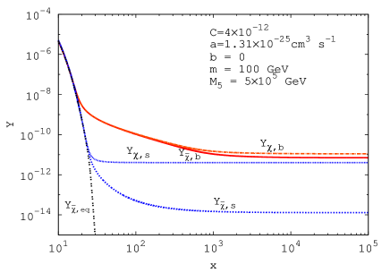
Figure 1: The relic abundances $Y_{\chi}$ and $Y_{\bar{\chi}}$ for particle and anti–particle as a function of the inverse–scaled temperature $x$ for $C=4\times 10^{-12}$, $m_{\chi}=100$ GeV, $g_{\chi}=2$, $g_{*}=90$, $a=1.31\times 10^{-25}$cm³ s^-1, $b=0$ for panels (a), (c), (e) and $a=1.38\times 10^{-24}$ cm³ s^-1, $b=0$ for panels (b), (d), (f); $M_{5}=5\times 10^{5}$ GeV in (a), (b); $M_{5}=10^{6}$ GeV in (c), (d) and $M_{5}=5\times 10^{6}$ GeV in (e), (f).

Fig.1 shows the relic abundance $Y_{\chi,\bar{\chi}}$ evolution as a function of the inverse–scaled temperature $x$ for particle and anti–particle for different cross sections and $M_{5}$ in brane cosmology scenario and standard scenario. This figure is plotted using the numerical solutions of Eqs.(13), (14). Here we take $C=4\times 10^{-12}$, $m_{\chi}=100$ GeV, $g_{\chi}=2$, $g_{*}=90$, $a=1.31\times 10^{-25}$ cm³ s^-1, $b=0$ for panels (a), (c), (e) and $a=1.38\times 10^{-24}$ cm³ s^-1, $b=0$ for panels (b), (d), (f); $M_{5}=5\times 10^{5}$ GeV in (a), (b); $M_{5}=10^{6}$ GeV in (c), (d) and $M_{5}=5\times 10^{6}$ GeV in (e), (f). The dot–dashed (red) line is the particle abundance $Y_{\chi,b}$ and the thick (red) line is the anti–particle abundance $Y_{\bar{\chi},b}$ in brane world cosmology; the dashed (blue) line is particle abundance $Y_{\chi,s}$ and dotted (blue) line is the anti–particle abundance $Y_{\bar{\chi},s}$ in the standard scenario. The double dotted (black) line is the equilibrium value $Y_{\bar{\chi},{\rm eq}}$ of the anti–particle abundance. Hubble expansion rate in brane world cosmology is larger than the Hubble expansion rate in the standard case. Particles and anti–particles freeze–out earlier than the standard cosmology. After decay of thermal equilibrium, there are more particles and anti–particles left in brane world cosmology than the standard case for appropriate cross section. Of course the extent of the increase depends on the cross sections and 5 dimensional scale $M_{5}$. The relic abundances $Y_{\chi,b}$ for particle $\chi$ and $Y_{\bar{\chi},b}$ for anti–particle $\bar{\chi}$ are larger than the standard case for panels (a) and (c) when the cross section is $a=1.31\times 10^{-25}$cm³ s^-1 for different $M_{5}$. We found for the same cross section the increase is larger for smaller $M_{5}$. When $M_{5}=5\times 10^{6}$ GeV in panel (e), the relic abundances for particle and anti–particle in brane world cosmology are almost same with the standard result. There is no enhancement for the relic density for particles and anti–particles. On the other hand, in brane world cosmology, for the larger cross section as $a=1.38\times 10^{-24}$cm³ s^-1 the particle abundance is almost kept in the same amount with the particle abundance in standard cosmology for different scaled $M_{5}$. This is shown in panels (b), (d) and (f). The anti–particle abundance is depressed for such kind of large cross section. It is more obvious for larger $M_{5}$ as in panel (f).

Using the same method as [4], we obtain the analytic solution of the relic density for asymmetric Dark Matter in brane world cosmology. We solve Eq.(14) for $\bar{\chi}$ density first and then using the relation $Y_{\chi}-Y_{\bar{\chi}}=C$ to find $Y_{\chi}$ easily. The Boltzmann equation (14) is rewritten as:

$$\frac{d\Delta_{\bar{\chi}}}{dx}=-\frac{dY_{\bar{\chi},{\rm eq}}}{dx}-\frac{\lambda\langle\sigma v\rangle}{\sqrt{x^{4}+k_{b}}}~{}\left[\Delta_{\bar{\chi}}(\Delta_{\bar{\chi}}+2Y_{\bar{\chi},{\rm eq}})+C\Delta_{\bar{\chi}}\right]\,,$$ (16)

where $\Delta_{\bar{\chi}}=Y_{\bar{\chi}}-Y_{\bar{\chi},{\rm eq}}$. We consider two extreme cases. At high temperature, $Y_{\bar{\chi}}$ closely tracks its equilibrium value $Y_{\bar{\chi},{\rm eq}}$ very well. $\Delta_{\bar{\chi}}$ is small, then we can neglect $d\Delta_{\bar{\chi}}/dx$ and $\Delta_{\bar{\chi}}^{2}$. The Boltzmann equation (16) then becomes

$$\frac{dY_{\bar{\chi},{\rm eq}}}{dx}=-\frac{\lambda\langle\sigma v\rangle}{\sqrt{x^{4}+k_{b}}}~{}\left(2\Delta_{\bar{\chi}}Y_{\bar{\chi},{\rm eq}}+C\Delta_{\bar{\chi}}\right)\,.$$ (17)

Repeating the same way as in [4], one obtains the solution for $\Delta_{\bar{\chi}}$

$$\Delta_{\bar{\chi}}\simeq\frac{2P\sqrt{x^{4}+k_{b}}}{\lambda\langle\sigma v\rangle\,(C^{2}+4P)}\,.$$ (18)

This solution is used to determine the freeze–out temperature $\bar{x}_{F}$ for $\bar{\chi}$.

In the second case, the production term $\propto Y_{\bar{\chi},{\rm eq}}$ can be ignored in the Boltzmann equation (16) for sufficiently low temperature, i.e. for $x>\bar{x}_{F}$, therefore

$$\frac{d\Delta_{\bar{\chi}}}{dx}=-\frac{\lambda\langle\sigma v\rangle}{\sqrt{x^{4}+k_{b}}}\left(\Delta_{\bar{\chi}}^{2}+C\Delta_{\bar{\chi}}\right)\,.$$ (19)

After integration of Eq.(19) from $\bar{x}_{F}$ to $\infty$, we obtain the final WIMP abundance. We have to be careful that the integration range is divided into two parts: one part is from $\bar{x}_{F}$ to $x_{t}$ where the brane world cosmology is applied. $x_{t}$ is the transition temperature at which point the standard cosmology recovers. It is given by $x_{t}=m_{\chi}/(0.51\times 10^{-9}M_{5}^{3/2})$ [7]. Second part is from $x_{t}$ to $\infty$ in which the standard cosmology is used. Again assuming $\Delta_{\chi}(\bar{x}_{F})\gg\Delta_{\chi}(\infty)$, we have

$$Y_{\bar{\chi}}(x\rightarrow\infty)=\frac{C}{\exp\left[1.32\,C\,m_{\chi}M_{\rm Pl}\,\sqrt{g_{*}}\,I(\bar{x}_{F},x_{t})\right]-1}\,,$$ (20)

where

$$I(\bar{x}_{F},x_{t}) = \int^{x_{t}}_{\bar{x}_{F}}\frac{\langle\sigma v\rangle}{\sqrt{x^{4}+k_{b}}}~{}dx+\int^{\infty}_{x_{t}}\frac{\langle\sigma v\rangle}{x^{2}}~{}dx$$ (21)

$$= a\left(\frac{1}{\bar{x}_{F}}\,{{}_{2}}F_{1}\left[\frac{1}{4},\frac{1}{2},\frac{5}{4},\frac{-k_{b}}{\bar{x}^{4}_{F}}\right]-\frac{1}{x_{t}}\,{{}_{2}}F_{1}\left[\frac{1}{4},\frac{1}{2},\frac{5}{4},\frac{-k_{b}}{x^{4}_{t}}\right]\right)$$ (22)

$$+ \frac{3b}{\sqrt{k_{b}}}\,\left[{\rm sinh}^{-1}\left(\frac{\sqrt{k_{b}}}{\bar{x}^{2}_{F}})-{\rm sinh}^{-1}(\frac{\sqrt{k_{b}}}{x^{2}_{t}}\right)\right]+\frac{a}{x_{t}}+\frac{3b}{x_{t}^{2}}\,.$$ (23)

Using equation (12), we obtain the relic abundance for $\chi$ particle,

$$Y_{\chi}(x\rightarrow\infty)=\frac{C}{1-\exp\left[-1.32\,C\,m_{\chi}M_{\rm Pl}\,\sqrt{g_{*}}\,I(x_{F},x_{t})\right]}\,.$$ (24)

Eqs.(20) and (24) are consistent with the constraint (12) if $x_{F}=\bar{x}_{F}$. Usually the final abundance is expressed as

$$\Omega_{\chi}h^{2}=\frac{m_{\chi}s_{0}Y_{\chi}(x\to\infty)h^{2}}{\rho_{\rm crit}}\,,$$ (25)

here $s_{0}=2.9\times 10^{3}~{}{\rm cm}^{-3}$ is the present entropy density, and $\rho_{\rm crit}=3M_{\rm Pl}^{2}H_{0}^{2}$ is the present critical density. The prediction for the present relic density for Dark Matter is then given by

$$\Omega_{\rm DM}h^{2} = 2.76\times 10^{8}~{}m_{\chi}\left[Y_{\chi}~{}(x\rightarrow\infty)+Y_{\bar{\chi}}~{}(x\rightarrow\infty)\right]$$

$$= \frac{2.76\times 10^{8}~{}m_{\chi}~{}C}{1-\exp\left[-1.32\,C\,m_{\chi}M_{\rm Pl}\,\sqrt{g_{*}}\,I(x_{F},x_{t})\right]}+\frac{2.76\times 10^{8}~{}m_{\chi}~{}C}{\exp\left[1.32\,C\,m_{\chi}M_{\rm Pl}\,\sqrt{g_{*}}\,I(\bar{x}_{F},x_{t})\right]-1}\,.$$

The freeze–out temperature for $\bar{\chi}$ is fixed using the standard method. It is assumed that the deviation $\Delta_{\bar{\chi}}$ is of the same order of the equilibrium value of $Y_{\bar{\chi}}$:

$$\xi Y_{\bar{\chi},{\rm eq}}(\bar{x}_{F})=\Delta_{\bar{\chi}}(\bar{x}_{F})\,,$$ (27)

where $\xi$ is a numerical constant of order unity. We find the approximate analytic result matches with the exact numerical result very well when we choose $\xi=\sqrt{2}-1$ [15].

3 Constraints on Parameter Space

Nine-year Wilkinson Microwave Anisotropy Probe (WMAP) observations give the Dark Matter relic density as [16]

$$\Omega_{\rm DM}h^{2}=0.1138\pm 0.0045\,,$$ (28)

where $\Omega_{\rm DM}$ is the Dark Matter (DM) density in units of the critical density, and $h=0.738\pm 0.024$ is the Hubble constant in units of 100 km s^-1 Mpc^-1. We use this result to find the constraints on the parameters in brane world cosmology for asymmetric Dark Matter. We use the following range for Dark Matter relic density,

$$0.10<\Omega_{\rm DM}h^{2}<0.12$$ (29)

The particle $\chi$ and anti–particle $\bar{\chi}$ density contribute together to the total Dark Matter density:

$$\Omega_{\rm DM}=\Omega_{\chi}+\Omega_{\bar{\chi}}\,.$$ (30)

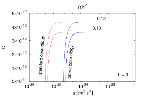
Figure 2: The allowed region in the $(a,C)$ plane for $b=0$ (left), and $(b,C)$ plane for $a=0$ (right) when the Dark Matter density $\Omega h^{2}$ lies between 0.10 and 0.12. Here we take $m_{\chi}=100$ GeV, $g_{\chi}=2$ and $g_{*}=90$, $M_{5}=10^{6}$ GeV. The dashed (red) line is for standard cosmology and the thick (blue) line is for brane cosmology.

Fig.2 shows the relation between the cross section parameters $a$, $b$ and asymmetry factor $C$ for the brane world cosmology and standard cosmology when the Dark Matter relic density $\Omega_{\rm DM}h^{2}$ lies between 0.10 and 0.12. Here we take $m_{\chi}=100$ GeV, $g_{\chi}=2$ and $g_{*}=90$, $M_{5}=10^{6}$ GeV. The dashed (red) lines are for the standard cosmology and the thick (blue) lines are for the brane world cosmological scenario. When $C$ is small as $C=0$ to $C=3.5\times 10^{-5}$, the cross section is almost independent of $C$. The reason is that for small $C$, the formulae for $Y_{\bar{\chi}}$, Eq.(20) and $Y_{\chi}$, Eq.(24) can be recovered to the result for symmetric Dark Matter in standard cosmology. When the asymmetry $C$ is large, e.g. $C=4.0\times 10^{-12}$, the particle and anti–particle are completely annihilated away and the relic density is independent of the cross section. On the other hand, for brane world cosmology, the cross section is larger than the standard cosmology for the observed value of Dark Matter. The reason is that in brane world cosmological scenario the interaction rate is larger than the standard scenario. Asymmetric Dark Matter particles need larger annihilation cross sections in order to fall in the observation range. In the left panel (a) of Fig.2, it is shown for s–wave annihilation cross sections from $a=3.99\times 10^{-26}$ ${\rm cm}^{3}{\rm s}^{-1}$ to $a=8.50\times 10^{-23}$ ${\rm cm}^{3}{\rm s}^{-1}$, the observed Dark Matter abundance is obtained for $C=0$ to $4.3\times 10^{-12}$. It is for the standard cosmology. The initial cross–section is increased to $a=1.93\times 10^{-25}$ ${\rm cm}^{3}{\rm s}^{-1}$ for the brane world cosmology. The similar behavior is seen in the right panel (b) of Fig.2. The cross section is increased evidently for brane world cosmology for both s–wave annihilation and p–wave annihilation cross sections to obtain the observed Dark Matter abundance.

For asymmetric Dark Matter, since in the beginning it is assumed that there is less anti–particle than the particle and at late time the anti–particle is completely annihilated away with the particle. Therefore the rest is the particle which made up the present total Dark Matter abundance in asymmetric Dark Matter case in standard cosmological scenario. Thus the asymmetric Dark Matter particle is supposed to be detected by direct detection. Usually the indirect detection is not available for the asymmetric Dark Matter. However, for asymmetric Dark Matter in nonstandard cosmological scenarios including quintessence, scalar–tensor model and brane world cosmology [9, 10, 11], the relic densities for both particle and anti–particle are increased in due to the enhanced Hubble expansion rate. Again for appropriate cross section, the relic density for both particle and anti–particle are almost in the same amount which is different from the standard cosmological scenario where the anti–particle relic density is depressed . Therefore the indirect detection is possible for nonstandard cosmology. However, for large annihilation cross section as $a=1.38\times 10^{-24}$ ${\rm cm}^{3}$ ${\rm s}^{-1}$, the indirect detection sigal can not be used. In Fig.1, it is shown when the cross section is as large as $a=1.38\times 10^{-24}$ ${\rm cm}^{3}$ ${\rm s}^{-1}$, the relic abundance of anti–particle is suppressed. Therefore there is not enough anti–particle left which can annihilate with particle to make up the indirect detection signal. Thus the indirect detection for asymmetric Dark Matter is available in conditionally where the annihilation cross section is not so large. As we showed in Fig.1, it depends on the scale of $M_{5}$, the mass of Dark Matter $m_{\chi}$, and most important is the cross section. In this article, it is assumed there is only particle and anti–particle annihilations. Therefore the abundant Dark Matter particle can not annihilate with itself to make the product particle which can be detected by indirect detection experiments.

The ratio of the relic abundance of the anti–particle to the particle as a function of the annihilation cross section $a$ is plotted in Fig.3 for $C=4\times 10^{-12}$. Here the dotted (black) line for asymmetric Dark Matter in standard cosmology and the solid (red) line in brane world cosmology. The decrease of the ratio is slower for brane world cosmology comparing to the standard cosmology as the cross section increases. For example, for the cross section value $a=2.50\times 10^{-25}$ ${\rm cm}^{3}$ ${\rm s}^{-1}$, the ratio is decreased to $2.2\times 10^{-5}$ for standard cosmology and $8.6\times 10^{-2}$ for brane world cosmology. We noticed that when the cross section increases, in both cases the abundances of anti–particles are suppressed. Therefore the indirect detection signal is not used for too large cross section in brane world cosmoloy for asymmetric Dark Matter.

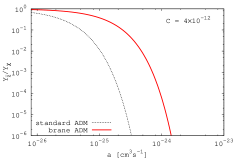
Figure 3: Ratio of the relic abundance of anti–particle and particle as a function of annihilation cross section $a$ in brane world cosmology and in the standard cosmology for the asymmetry factor $C=4\times 10^{-12}$. The dotted (black) line is for the asymmetric Dark Matter (ADM) in standard cosmology and the solid (red) line is for the asymmetric Dark Matter in brane world cosmology. Here $b=0$, $m_{\chi}=100$ GeV and $C=4\times 10^{-12}$, $M_{5}=10^{6}$ GeV, $g_{\chi}=2$, $g_{*}=90$.

4 Summary and Conclusions

In this paper we investigated the relic abundance of asymmetric WIMP Dark Matter in brane world cosmology. For asymmetric Dark Matter the particles and anti–particles are different from each other. It is assumed the asymmetry starts well before the epoch of thermal decoupling of the WIMPs. The asymmetric Dark Matter particles and anti–particles freeze–out earlier than the standard cosmology due to the enhanced Hubble rate in brane world cosmology. This leads to the increase of the relic density of asymmetric Dark Matter particles.

We found that the relic densities of both particles and anti–particles are increased in brane world cosmology. The size of the increase depends on the 5 dimensional Planck mass scale $M_{5}$ and the cross sections. The increases are more sizable for smaller $M_{5}$ for the same cross section. When $M_{5}$ is large, e.g. $M_{5}=5\times 10^{6}$ GeV, the case in the standard cosmology is recovered. For larger annihilation cross section as $a=1.38\times 10^{-24}{\rm cm^{3}}$ ${s^{-1}}$, the particle abundance in brane world cosmology is the same with the particle abundance in standard cosmology for different $M_{5}$. The antiparticle abundance is suppressed.

We used the WMAP data to give the constraints on the cross section and asymmetry factor $C$ in brane world cosmology. We showed that the indirect detection signal is conditionally used for asymmetric Dark Matter in brane world cosmology.

The result which is obtained in our work is important to understand the relic abundance of asymmetric Dark Matter in the early universe before Big Bang Nucleosynthesis. If we know the annihilation cross section in the brane world cosmology, we can find the relic density of Dark Matter in this scenario. It has important effect to investigate the early universe before BBN.

References

- [1] S. Nussinov, Phys. Lett. B 165, 55 (1985); K. Griest and D. Seckel. Nucl. Phys. B 283, 681 (1987); R. S. Chivukula and T. P. Walker, Nucl. Phys. B 329, 445 (1990); D. B. Kaplan, Phys. Rev. Lett. 68, 742 (1992); D. Hooper, J. March-Russell and S. M. West, Phys. Lett. B 605, 228 (2005) [arXiv:hep-ph/0410114]; JCAP 0901 (2009) 043 [arXiv:0811.4153v1 [hep-ph]]; H. An, S. L. Chen, R. N. Mohapatra and Y. Zhang, JHEP 1003, 124 (2010) [arXiv:0911.4463 [hep-ph]]; T. Cohen and K. M. Zurek, Phys. Rev. Lett. 104, 101301 (2010) [arXiv:0909.2035 [hep-ph]]. D. E. Kaplan, M. A. Luty and K. M. Zurek, Phys. Rev. D 79, 115016 (2009) [arXiv:0901.4117 [hep-ph]]; T. Cohen, D. J. Phalen, A. Pierce and K. M. Zurek, Phys. Rev. D 82, 056001 (2010) [arXiv:1005.1655 [hep-ph]]; J. Shelton and K. M. Zurek, Phys. Rev. D 82, 123512 (2010) [arXiv:1008.1997 [hep-ph]];
- [2] A. Belyaev, M. T. Frandsen, F. Sannino and S. Sarkar, Phys. Rev. D 83, 015007 (2011) [arXiv:1007.4839].
- [3] M. L. Graesser, I. M. Shoemaker and L. Vecchi, [arxiv:1103.2771 [hep-ph]].
- [4] H. Iminniyaz, M. Drees and X. Chen, JCAP 1107, 003 (2011) [arXiv:1104.5548 [hep-ph]].
- [5] P. Salati, Phys. Lett. B 571, 121 (2003) [astro-ph/0207396].
- [6] R. Catena, N. Fornengo, A. Masiero, M. Pietroni and F. Rosati, Phys. Rev. D 70, 063519 (2004) [arXiv:astro-ph/0403614].
- [7] E. Abou El Dahab and S. Khalil, JHEP 0609 (2006) 042 [hep-ph/0607180].
- [8] N. Okada and O. Seto, Phys. Rev. D 70 (2004) 083531 [hep-ph/0407092].
- [9] H. Iminniyaz and X. Chen, Astropart. Phys. 54, 125 (2014) [arXiv:1308.0353 [hep-ph]].
- [10] G. B. Gelmini, J. H. Huh and T. Rehagen, arXiv:1304.3679 [hep-ph].
- [11] S. Z. Wang, H. Iminniyaz and M. Mamat, arXiv:1503.06519 [hep-ph].
- [12] M. T. Meehan and I. B. Whittingham, JCAP 1406, 018 (2014) [arXiv:1403.6934 [astro-ph.CO]].
- [13] O. Lahav and A. R. Liddle, arXiv:1401.1389 [astro-ph.CO].
- [14] M. Ackermann et al. [Fermi-LAT Collaboration], Phys. Rev. Lett. 107, 241302 (2011) [arXiv:1108.3546 [astro-ph.HE]].
- [15] R. J. Scherrer and M. S. Turner, Phys. Rev. D 33, 1585 (1986), Erratum-ibid. D 34, 3263 (1986).
- [16] G. Hinshaw et al. [WMAP Collaboration], Astrophys. J. Suppl. 208, 19 (2013); C. L. Bennett et al. [WMAP Collaboration], Astrophys. J. Suppl. 208, 20 (2013).