Testing a generalized cubic Galileon gravity model with the Coma Cluster

Abstract

We obtain a constraint on the parameters of a generalized cubic Galileon gravity model exhibiting the Vainshtein mechanism by using multi-wavelength observations of the Coma Cluster. The generalized cubic Galileon model is characterized by three parameters of the turning scale associated with the Vainshtein mechanism, and the amplitude of modifying a gravitational potential and a lensing potential. X-ray and Sunyaev–Zel’dovich (SZ) observations of the intra-cluster medium are sensitive to the gravitational potential, while the weak-lensing (WL) measurement is specified by the lensing potential. A joint fit of a complementary multi-wavelength dataset of X-ray, SZ and WL measurements enables us to simultaneously constrain these three parameters of the generalized cubic Galileon model for the first time. We also find a degeneracy between the cluster mass parameters and the gravitational modification parameters, which is influential in the limit of the weak screening of the fifth force.

1 Introduction

Modifications of gravity theory is an interesting approach to explaining the accelerated expansion of the universe. However, any covariant modification of general relativity introduces additional degrees of freedom, giving rise to a fifth force. This is strictly constrained by gravity tests in the solar system. Solar system experiments [1, 2] are in excellent agreement with general relativity, requiring that this additional degree of freedom be hidden on the scale of the solar system. Such a process is referred to as a “screening mechanism,” which is key for a viable modified gravity model. In general, this screening mechanism works in high-density regions where the matter density contrast is nonlinear. However, this does not work on large cosmological scales. A screening mechanism that characterizes viable modified gravity models is an important feature to be tested with observations.

The chameleon mechanism [3, 4] is a screening mechanism that works in an $f(R)$ gravity model and the chameleon gravity model [5, 6, 7]. In these models, a scalar degree of freedom that gives rise to the fifth force is screened in a high-density region due to coupling with matter. The chameleon gravity model and an $f(R$) model can be viable owing to the chameleon mechanism [8]. The Vainshtein mechanism [9] is another relevant screening mechanism, which is exhibited in the Dvali–Gabadaze–Porrati (DGP) model [10, 11], the simplest cubic Galileon model ([12, 13, 14, 15], see also the appendix), and its generalized version [16, 17]. The DGP model is an archetypal modified gravity model developed in the context of the brane-world scenario. There are two branches of solutions in the DGP model. The self-acceleration branch DGP (sDGP) model [18, 19, 20] includes a mechanism to explain self-acceleration in the late universe, while the normal branch DGP (nDGP) model [21, 22, 23] with a cosmological constant is a healthy modified gravity model avoiding the ghost problem [24, 25]. The simplest cubic Galileon model is also a typical modified gravity model that explains self-acceleration of the universe while avoiding the ghost problem. Our generalized cubic Galileon model is a generalized version of the simplest cubic Galileon model that retains important features and contains the DGP models. In these models, a scalar field giving rise to a fifth force is screened due to self-interaction on small scales where density perturbations become nonlinear.

Galaxy clusters provide a unique laboratory for testing modified gravity models exhibiting screening mechanisms, because they are objects on the borderline between linear and nonlinear scales, that is, between non-screened and screened scales. The authors of [26, 27, 28] have investigated a cosmological constraint on the chameleon gravity model using galaxy clusters. They put a constraint on the turning scale and the amplitude of the fifth force at large scales. The authors of [29, 30] have investigated a constraint on a generalized Galileon model exhibiting the Vainshtein mechanism, using an observed weak-lensing profile of clusters. They put a constraint on the turning scale and the amplitude of modification of the lensing potential.

The purpose of the present paper is twofold. One purpose is a generalization of the methodology for testing a modified gravity model with a galaxy cluster. In the present paper, we consider a generalized cubic Galileon model. Within the quasi-static approximation, the generalized cubic Galileon model is effectively characterized by three parameters, $\mu_{\rm G}$, $\mu_{\rm L}$ and $\epsilon$. Detailed definitions are given later, but, broadly, $\mu_{\rm G}$ and $\mu_{\rm L}$ are parameters that modify the effective amplitude of the gravitational potential and the lensing potential in the non-screened region, while $\epsilon$ determines the turning scale from the non-screened region to the screened region due to the Vainshtein mechanism. The parameters $\mu_{\rm G}$ are constrained by observations of the gas distribution, in particular an X-ray surface brightness profile and the SZ effect [31]. However, the parameter $\mu_{\rm L}$ is only constrained by observations of lensing measurements. Therefore, a combination of observations of gas distribution and the lensing signal is essential to put a constraint on the three parameters characterizing the modified gravity model. We demonstrate how a combination of multi-wavelength observations of a cluster is useful to put a constraint on a generalized Galileon model.

The other purpose is improvement of the analysis in [27] using new X-ray data [32, 33] and lensing [34] observations of the Coma Cluster. In our method of testing gravity with a galaxy cluster, the modeling of the gas distribution is important. A basic assumption of the model for the gas distribution is hydrostatic equilibrium, that is, a balance between the gas pressure gradient force and the gravitational force. In the region where the fifth force is influential, the condition of the hydrostatic equilibrium is changed, and the gas density profile is modified. However, in general, galaxy clusters are dynamically evolving, and a deviation from the equilibrium could be influential. Therefore, we first check the consistency of our model by comparing theoretical predictions with various observations of the Coma Cluster, including the new X-ray data and lensing measurements.

This paper is organized as follows: In Section 2, we first review our model for the dark matter and gas distribution of a galaxy cluster within Newtonian gravity. We demonstrate how well our model fits observations of the Coma Cluster in Section 3. We also validate our model against the influence of non-thermal pressure. In Section 4, we introduce a generalized cubic Galileon model, and explain the modification of our model by the fifth force of the scalar field. In Section 5, we discuss degeneracies on parameters and systematic errors focusing on special circumstance of using the Coma Cluster. Section 6 is devoted to a summary and conclusions. Throughout this paper, we adopt $\Omega_{\rm m0}=0.3$, $\Omega_{\Lambda}=0.7$ and $H_{0}=70{\rm km/s/Mpc}$, and we follow the convention $(-,+,+,+)$.

2 Modeling of cluster profiles

We review our model for the dark matter and gas density distribution connecting with observational quantities, X-ray brightness, the SZ effect temperature profile, and the weak-lensing profile (see also [27, 29]). Our model is based on an assumption of hydrostatic equilibrium, but we also take the possible influence of non-thermal pressure into account. In this section, we first consider the case of Newtonian gravity.

2.1 Mass profile

We employ a universal mass density profile, namely the Navarro–Frenk–White (NFW) profile [35], motivated by predictions of numerical simulations,

$$\rho(r)=\frac{\rho_{\rm s}}{r/r_{\rm s}(1+r/r_{\rm s})^{2}},$$ (2.1)

where $\rho_{\rm s}$ and $r_{\rm s}$ are the normalization and the scale radius, respectively. The mass within the radius $r$ is given by $M(<r)=4\pi\int^{r}_{0}drr^{2}\rho(r)=4\pi\rho_{\rm s}r_{\rm s}^{3}m(r),$ with $m(r)=\ln(1+r/r_{\rm s})-r/r_{\rm s}/(1+r/r_{\rm s})$. We introduce the concentration parameter $c$ and the virial mass $M_{\rm vir}$ instead of $\rho_{\rm s}$ and $r_{\rm s}$,

$$c=\frac{r_{\rm vir}}{r_{\rm s}},$$ (2.2)

$$M_{\rm vir}\equiv M(<r_{\rm vir})=\frac{4\pi}{3}r^{3}_{\rm vir}\Delta_{\rm c}\rho_{\rm c}(z)$$ (2.3)

with the virial radius $r_{\rm vir}$. Here, $\rho_{\rm c}$ is the critical density at the redshift $z$, and $\Delta_{\rm c}=100$ is the overdensity contrast determined by the spherical collapse model [36].

2.2 Gas profile with hydrostatic equilibrium

We first assume hydrostatic equilibrium between the gas pressure gradient and the gravitational force in galaxy clusters as

$$\frac{1}{\rho_{\rm gas}}\frac{dP_{\rm tot}}{dr}=-\frac{d\Psi}{dr},$$ (2.4)

where $\rho_{\rm gas}$ is the gas density, $P_{\rm tot}=P_{\rm th}+P_{\rm nth}$ is the sum of the thermal pressure, $P_{\rm th}$ and the non-thermal pressure, $P_{\rm nth}$ (see below for details), and $\Psi$ is the gravitational potential. We employ three assumptions to describe the gas physics. First, the equation of state for the gas components, $P_{\rm th}=n_{\rm gas}kT_{\rm gas}$, where $n_{\rm gas}$ and $T_{\rm gas}$ are the number density and the temperature of the total gas component, respectively. Second, the temperature of electrons is the same as that of the gas, $T_{\rm e}=T_{\rm gas}$. Third, the electron pressure satisfies $P_{\rm e}=n_{\rm e}kT_{\rm gas}$ with the electron number density $n_{\rm e}=(2+\mu)n_{\rm gas}/5$, where $\mu=0.59$ is the mean molecular weight. In the present paper, for the electron temperature we assume the functional form

$$T_{\rm e}(r)=T_{0}\left[1+\left(\frac{r}{r_{\rm 1}}\right)^{b_{1}}\right]^{-b_{2}/b_{1}},$$ (2.5)

where $T_{0}$, $b_{1}$, $b_{2}$ and $r_{1}$ are parameters. Integrating (2.4) with (2.5), we obtain the electron pressure profile

$$P_{\rm e}(r)=n_{0}T_{0}\exp\left(\int_{0}^{r}dr\frac{\mu m_{\rm p}}{kT_{\rm e}(r)}\left[-\frac{GM(<r)}{r^{2}}\right]\right),$$ (2.6)

and the electron number density $n_{\rm e}(r)=P_{\rm e}(r)/kT_{\rm e}(r)$, where $n_{0}$ is the normalization parameter of the electron number density, $n_{\rm e}$. In deriving equation (2.6), we use the relation, $\rho_{\rm gas}=\mu m_{\rm p}n_{\rm gas}$, where $m_{\rm p}$ is the proton mass. Equation (2.6) is the case of the absence of non-thermal pressure; the case including non-thermal pressure is described below.

Thus our gas distribution model includes 7 parameters ($M_{\rm vir}$,$c$,$n_{0}$,$T_{0}$,$b_{1}$,$b_{2}$,$r_{1}$). Using our model of the three-dimensional profiles, we construct the observables for the observations of X-ray and the cosmic microwave background (CMB) temperature distortion. The X-ray emission from clusters are dominated by the bremsstrahlung and line emission caused by the ionized gas. For the X-ray observable, we define the X-ray brightness as $B_{\rm X}\equiv{\it norm}/{\it area}$, where norm is the spectrum normalization obtained from XSPEC software [37] adopting the APEC emission spectrum [38], and area is the area of the spectrum. The spectrum normalization is given by ${\it norm}\propto\int n_{\rm e}n_{\rm H}dV$, where $n_{\rm H}=0.86n_{\rm e}$ is the hydrogen number density and $V$ is the volume of the spectrum. Then, we write the X-ray brightness as

$$B_{\rm X}(r_{\perp})=\frac{10^{-14}}{4\pi(1+z)^{2}}\int n_{\rm e}(r)n_{\rm H}(r)dz~{}[{\rm cm^{-5}/arcmin^{2}}],$$ (2.7)

where $r_{\perp}$ is the radius perpendicular to the line-of-sight direction, which is related with $r$ and $z$ as $r=\sqrt{r_{\perp}^{2}+z^{2}}$. The CMB temperature distortion is caused by CMB photons passsing through clusters and being scttered by electrons in clusters, can be expressed as the difference between the averaged CMB temperature and the observed CMB temperature, $\Delta T_{\rm SZ}$, or $y$-parameter,

$$y(r_{\perp})=-\frac{\Delta T_{\rm SZ}}{2T_{\rm CMB}}=\frac{\sigma_{\rm T}}{m_{\rm e}}\int P_{\rm e}(r)dz,$$ (2.8)

where $T_{\rm CMB}=2.725$ K is the CMB temperature, $\sigma_{\rm T}$ is the Thomson cross section, $m_{\rm e}$ is the electron mass.

2.3 Shear profile by gravitational weak-lensing

We consider a spatially flat cosmological background, and work with the cosmological Newtonian gauge, whose line element is written as

$$ds^{2}=-(1+2\Psi)dt^{2}+a(t)^{2}(1+2\Phi)d{\bf x}^{2},$$ (2.9)

where $a(t)$ is the scale factor, and $\Psi$ and $\Phi$ are the gravitational and curvature potentials, respectively. The propagation of light is determined by the lensing potential $(\Phi-\Psi)/2$, which means that the weak-lensing signal is determined by $(\Phi-\Psi)/2$. For example, the convergence is given by

$$\kappa=-\frac{1}{2}\int_{0}^{\chi}d\chi^{\prime}\frac{(\chi-\chi^{\prime})\chi^{\prime}}{\chi}\triangle^{\rm(2D)}(\Phi-\Psi),$$ (2.10)

where $\chi$ is the comoving distance and $\triangle^{\rm(2D)}$ is the comoving two-dimensional Laplacian. For the case of general relativity, we may set $\triangle\Psi=-\triangle\Phi=4\pi Ga^{2}\rho$. Then, using the thin lens approximation, (2.10) reduces to

$$\kappa=\frac{(\chi_{\rm S}-\chi_{\rm L})\chi_{\rm L}}{\chi_{\rm S}}\int_{0}^{\chi_{\rm S}}d\chi^{\prime}\left[4\pi G\rho(r^{\prime})\right]a_{\rm L}^{2},$$ (2.11)

where $\chi_{\rm L}$ and $\chi_{\rm S}$ denote the comoving distance between the observer and lens and that between the observer and the source, respectively, and $a_{\rm L}=1/(1+z_{\rm L})$ is the scale factor specified by the redshift of the lens object $z_{\rm L}$. For a spherically symmetric cluster, (2.11) is represented as

$$\kappa(r_{\perp})=\frac{2}{\Sigma_{\rm c}}\int_{0}^{\infty}dz\rho(r)$$ (2.12)

with the physical coordinate $r=\sqrt{r_{\perp}^{2}+z^{2}}$. We define $\Sigma_{\rm c}=\chi_{\rm S}/[{4\pi G}{(\chi_{\rm S}-\chi_{\rm L})\chi_{\rm L}a_{\rm L}}]$. We then define the reduced shear

$$g_{+}(r_{\perp})\equiv\frac{\gamma_{+}(r_{\perp})}{1-\kappa(r_{\perp})},$$ (2.13)

where $\gamma_{+}(r_{\perp})$ is the tangential shear, which is related with the convergence as

$$\gamma_{+}(r_{\perp})=\bar{\kappa}(<r_{\perp})-\kappa(r_{\perp}),$$ (2.14)

with

$$\bar{\kappa}(<r_{\perp})\equiv\frac{2}{r_{\perp}^{2}}\int_{0}^{r_{\perp}}dr_{\perp}^{\prime}r_{\perp}^{\prime}\kappa(r_{\perp}^{\prime}).$$ (2.15)

For the NFW profile, the convergence is given by [39] as

$$\kappa_{\rm nfw}(x)=\left\{\begin{array}[]{ll}\dfrac{2r_{\rm s}\rho_{\rm s}}{\Sigma_{\rm c}(x^{2}-1)}\left[1-\dfrac{2}{\sqrt{1-x^{2}}}\text{arctanh}\sqrt{\dfrac{1-x}{1+x}}\right],&\quad(x<1)\\ \dfrac{2r_{\rm s}\rho_{\rm s}}{3\Sigma_{\rm c}},&\quad(x=1)\\ \dfrac{2r_{\rm s}\rho_{\rm s}}{\Sigma_{\rm c}(x^{2}-1)}\left[1-\dfrac{2}{\sqrt{x^{2}-1}}\text{arctan}\sqrt{\dfrac{x-1}{1+x}}\right],&\quad(x>1)\end{array}\right.$$ (2.19)

$$\bar{\kappa}_{\rm nfw}(<x)=\left\{\begin{array}[]{ll}\dfrac{4r_{\rm s}\rho_{\rm s}}{\Sigma_{\rm c}x^{2}}\left[\dfrac{2}{\sqrt{1-x^{2}}}\text{arctanh}\sqrt{\dfrac{1-x}{1+x}}+\ln\left(\dfrac{x}{2}\right)\right],&\quad(x<1)\\ \dfrac{4r_{\rm s}\rho_{\rm s}}{\Sigma_{\rm c}}\left[1+\ln\left(\dfrac{1}{2}\right)\right],&\quad(x=1)\\ \dfrac{4r_{\rm s}\rho_{\rm s}}{\Sigma_{\rm c}x^{2}}\left[\dfrac{2}{\sqrt{x^{2}-1}}\text{arctan}\sqrt{\dfrac{x-1}{1+x}}+\ln\left(\dfrac{x}{2}\right)\right],&\quad(x>1)\end{array}\right.$$ (2.23)

with $x=r/r_{\rm s}$.

Here, we assume that the source galaxies have random orientation of ellipticity $\epsilon_{\rm S}$, the average of which is $\langle\epsilon_{\rm S}\rangle=0$. When we observe the tangential ellipticity of the source galaxies $\epsilon_{\rm obs.}$, the average is given by $\langle\epsilon_{\rm obs.}\rangle=g_{+}$. Hereafter, we assume that the redshift of the source galaxies is $\langle z_{\rm S}\rangle=0.6$, but the results are not influenced by the redshift of the source galaxies for nearby clusters.

3 Consistency test with Newtonian gravity

In the present paper, we use Coma Cluster observations. The Coma Cluster is one of the best observed nearby clusters, and has redshift $z=0.0236$. The X-ray distribution [32, 33, 40, 41, 42, 43, 44, 45, 46, 47], the SZ effect [48] and the weak-lensing measurement [49, 34] have been reported. These observations revealed that the Coma Cluster has substructures and orientation dependence on the gas temperature profiles. The Coma Cluster is thus an unrelaxed system. However, we will show that our model based on the hydrostatic equilibrium fits the data of the X-ray brightness profiles [32, 33], the SZ effect profile from the Planck measurement [48], and the weak-lensing profile by Subaru observations [34]. In general, the assumption of hydrostatic equilibrium holds only at the intermediate region of clusters, because of the cooling of the gas at the innermost region and the environmental effects at the outermost region. Then we use data points in the range $200\ {\rm kpc}$ to $1.5\ {\rm Mpc}$ to get rid of systematic effects from the innermost and outermost regions of the cluster.

In this work, we use the observational data of the XMM-Newton [32, 33], which are different from those used in a previous paper [27]. In that paper, the weak-lensing profile is not used; only the parameters $M_{\rm vir}$ and $c$ are used as a prior profile from [49]. However, use of the weak-lensing profile is essential to our analysis of the generalized Galileon model.

To address the theoretical predictions in the previous section with observations of the Coma Cluster, we introduce the chi-squared by summing the chi-squared for each observation as

$$\chi_{\rm XB+SZ+WL}^{2} =\chi_{\rm XB}^{2}+\chi_{\rm SZ}^{2}+\chi_{\rm WL}^{2},$$ (3.1)

where

$$\chi_{\rm XB}^{2}=\sum_{i}\frac{(B_{\rm X}(r_{i})-B_{{\rm X},i}^{\rm obs.})^{2}}{(\Delta B_{{\rm X},i}^{\rm obs.})^{2}},$$ (3.2)

$$\chi_{\rm SZ}^{2}=\sum_{i}\frac{(y(r_{\perp,i})-y_{i}^{\rm obs.})^{2}}{(\Delta y_{,i}^{\rm obs.})^{2}},$$ (3.3)

$$\chi_{\rm WL}^{2}=\sum_{i}\frac{(g_{+}(r_{\perp,i})-g_{+,i}^{\rm obs.})^{2}}{(\Delta g_{+,i}^{\rm obs.})^{2}},$$ (3.4)

are the chi-square values for the X-ray brightness, the SZ effect and the weak-lensing, respectively. We note that the covariance of errors is not taken into account in our analysis and leave it for future work to study how the observational systematics affect our analysis.

We perform an MCMC analysis using modified Monte Python code [50] that employs a Metropolis–Hastings [51, 52] sampling algorithm. This analysis includes 5 parameters with the chi-squared (3.1), $\chi^{2}_{\rm BX+SZ+WL}$. We require Gelman–Rubin statistics [53] of ${\cal R}-1<0.001$ for each parameter to ensure convergence of our runs. The black dashed curve in each panel of figure 1 shows the best-fit profiles for the Newtonian gravity. The minimum value of the chi-squared is $\chi_{\rm XB+SZ+WL}^{2}/{\rm d.o.f.}=58/44$, and the 2-dimensional marginalized contours of the different combinations between the model parameters are shown in figure 4.

Table 1: Best-fitting parameters and 1-dimensional marginalized constraints ($68$% CL) to characterize the gas and lensing profiles. To avoid degeneracy between parameters, we fix $b_{1}$ and $b_{2}$ simply. Our results do not depend on whether these parameters are fixed or not. This table shows the results for the Newtonian gravity (second column) and the generalized Galileon model with all modification parameters (third column). The minimum chi-squared and the number of degrees of freedom, d.o.f. $=$ (number of data points) $-$ (number of model parameters), are listed at the bottom of each column.

Parameter	Newtonian gravity	Modified gravity (full parameters)
$M_{\rm vir}$	${1.08}^{+0.06}_{-0.06}\times 10^{15}~{}M_{\odot}$	${1.04}^{+0.14}_{-0.06}\times 10^{15}~{}M_{\odot}$
$c$	${3.59}^{+0.23}_{-0.23}$	${3.64}^{+0.21}_{-0.30}$
$n_{0}$	${6.14}^{+0.28}_{-0.26}\times 10^{-3}{\rm/cm^{3}}$	${6.17}^{+0.26}_{-0.31}\times 10^{-3}{\rm/cm^{3}}$
$T_{0}$	${6.36}^{+0.11}_{-0.12}~{}{\rm keV}$	${6.35}^{+0.13}_{-0.11}~{}{\rm keV}$
$b_{1}$	${2.6}$ (fixed)	${2.6}$ (fixed)
$b_{2}$	${0.5}$ (fixed)	${0.5}$ (fixed)
$r_{1}$	${0.74}^{+0.06}_{-0.06}~{}{\rm Mpc}$	${0.75}^{+0.06}_{-0.07}~{}{\rm Mpc}$
$\epsilon^{\prime}$	-	${0.43}$
$\mu_{\rm G}^{\prime}$	-	${0.24}$
$\mu_{\rm L}^{\prime}$	-	${0.55}$
Minimum $\chi^{2}$/d.o.f.	${58/44}$	${57/41}$

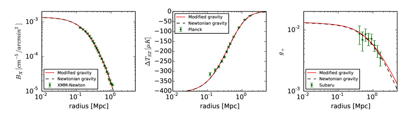
Figure 1: Best-fit profiles in the frameworks of Newtonian gravity (black dashed curve) and the generalized Galileon model (red solid curve), and the observational results. The best-fit parameters are listed in Table 1. Left panel: The X-ray surface brightness from the XMM-Newton observations [32, 33]. The errors bars are composed of the Poisson noise and systematic errors that we here assume as 5%. Center panel: The SZ temperature profile from the Planck measurements [48]. Right panel: The weak-lensing profile from the Subaru observations [49].

Non-thermal pressure possibly caused by turbulent gas and bulk motion causes a systematic error when comparing observations of clusters. The authors estimated the fraction of non-thermal pressure in the Coma Cluster [54], which can be larger than that of the thermal pressure by $10$ percent. Here, we estimate how non-thermal pressure affects our fitting based on an estimation with a numerical simulation. To this end, we estimate the hydrostatic masses by comparison with the X-ray brightness and SZ effect profiles of the Coma Cluster. Here we define the non-thermal fraction $f_{\rm nth}$ by $f_{\rm nth}\equiv{P_{\rm nth}}/({P_{\rm nth}+P_{\rm th}}),$ where $P_{\rm nth}$ and $P_{\rm th}$ are the non-thermal pressure and the thermal pressure, respectively. In the case including non-thermal pressure, the thermal pressure is replaced by $P_{\rm th}=(1-f_{\rm nth})P_{\rm tot}$. We consider the following non-thermal pressure fraction as a function of the radius,

$$f_{\rm nth}(r)=\alpha_{\rm nt}(1+z)^{\beta_{\rm nt}}\left(\frac{r}{r_{500}}\right)^{n_{\rm nt}}\left(\frac{M_{200}}{3\times 10^{14}M_{\odot}}\right)^{n_{\rm M}},$$ (3.5)

which is a theoretical prediction with numerical simulations in Ref. [55, 56]. $r_{500}$ and $M_{200}$ mean the radius and mass at the radius where the matter density in the galaxy cluster is 500 and 200 times of the critical density, respectively. In the present paper we adopt $(\alpha_{\rm nt},~{}\beta_{\rm nt},~{}n_{\rm nt},n_{\rm M})=(0.18,0.5,0.8.0.2)$, which are the best-fit values in [56] consistent with those in [54].

The best-fit profile in the presence of non-thermal pressure is not significantly altered, compared with the best-fit profile in the absence of non-thermal pressure. Figure 2 shows the enclosed mass profiles as a function of radius. The gray-hatched region is the 1$\sigma$ uncertainty interval for the lensing mass. The blue-solid and red-solid regions show the 1$\sigma$ uncertainty intervals for hydrostatic masses fitted without and with non-thermal pressure, respectively. The hydrostatic mass estimates are in good agreement with the lensing mass, regardless of the inclusion of the non-thermal pressure components. This shows that our fitting method is not affected by non-thermal pressure, so we do not consider the non-thermal effect when putting a constraint on the modified gravity in the next section.

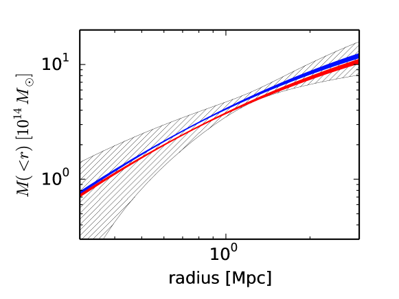
Figure 2: Spherical masses enclosed within the radii. The gray-hatched region denotes the $1\sigma$ uncertainty interval for the lensing mass determined solely by weak-lensing analysis [49]. The blue-solid and red-solid regions denote the $1\sigma$ uncertainty intervals for hydrostatic masses without and with the non-thermal pressure component, respectively, determined by our joint-fit method. The hydrostatic and lensing masses agree with each other, irrespective of the presence of a non-thermal pressure component.

4 Testing the generalized Galileon gravity model

We here consider the generalized cubic Galileon model, with action given by [57],

$$S=\int d^{4}x\sqrt{-g}\Bigl{[}G_{4}(\phi)R+K(\phi,X)-G_{3}(\phi,X)\square\phi+{\cal L}_{\rm m}\Bigr{]},$$ (4.1)

where $K(\phi,X)$, $G_{3}(\phi,X)$ and $G_{4}(\phi)$ are arbitrary functions depending on the scalar field $\phi$ and its kinetic term $X\equiv-(\partial\phi)^{2}/2$ and ${\cal L_{\rm m}}$ is the matter Lagrangian. This model is a non-minimal coupling version of the kinetic gravity braiding mode [58], and a subclass of the most general second-order scalar-tensor theory [59, 60, 61] with $G_{4X}=G_{5}=0$, where $G_{4X}\equiv\partial G_{4}/\partial X$. The simplest cubic Galileon model is the case with $K=-X$, $G_{3}\propto X$, and $G_{4}=M_{\rm Pl}^{2}/2$, where $M_{\rm Pl}^{2}=1/(8\pi G)$ is the Planck mass. The DGP model is originally a 5-dimensional brane-world model, however, it can be effectively described as a Galileon model. Note that the DGP model has two branches of cosmological solutions, the self-accelerating branch (sDGP) model [18, 19] and the normal branch DGP (nDGP) model [21]. The relation between the generalized Galileon model and the specific models are summarized in the appendix.

We consider perturbations of space-time metric and scalar field. We choose the Newtonian gauge for the space-time metric (2.9). Assuming spherical symmetry of the system, within the sub-horizon scale with the quasi-static approximation keeping with the Vainshtein feature, the equations for the gravity and the scalar field lead to [17]

$$\frac{d\Psi}{dr} =\frac{GM(<r)}{r^{2}}-(\alpha+\xi)\frac{dQ}{dr},$$ (4.2)

$$\frac{d\Phi}{dr} =-\frac{GM(<r)}{r^{2}}+\xi\frac{dQ}{dr},$$ (4.3)

$$\frac{dQ}{dr} =\frac{r}{4\lambda^{2}}\left(1-\sqrt{1+\frac{8G\lambda^{2}\zeta M(<r)}{r^{3}}}\right),$$ (4.4)

where $Q({\bf x})$ is perturbation of the scalar field defined by $\phi(t,{\bf x})=\phi(t)(1+Q({\bf x}))$, and $M(<r)\equiv 4\pi\int_{0}^{r}dr^{\prime}{r^{\prime}}^{2}\rho(r^{\prime})$ is the enclosed mass of the halo within the physical radius $r$. Note that the perturbed values $\Psi$, $\Phi$ and $Q$ in (4.2)$\sim$(4.4) are written in the physical coordinate. In (4.2)$\sim$(4.4), we introduce free model parameters $\alpha$, $\xi$, $\zeta$ and $\lambda^{2}$, which are determined by the arbitrary functions $K$, $G_{3}$ and $G_{4}$. The expressions for $\alpha$, $\xi$, $\zeta$ and $\lambda^{2}$ are given in the appendix A. The explicit expressions for the simplest cubic Galileon, the sDGP and the nDGP models are also presented there.

Here, we define the Vainshtein radius $r_{\rm V}$ as

$$r_{\rm V}\equiv[8G\lambda^{2}\zeta M_{\rm vir}]^{1/3}=\bigg{[}{8G\epsilon^{2}M_{\rm vir}\over H_{0}^{2}}\biggr{]}^{1/3},$$ (4.5)

where we define $\epsilon=\sqrt{H_{0}^{2}\lambda^{2}\zeta}$ using the Hubble constant $H_{0}$. For $r\ll r_{\rm V}$, the scalar field can be negligible compared with the Newton potential, so Newtonian gravity is recovered. For $r\gg r_{\rm V}$ the scalar field cannot be negligible, and we have

$$\frac{d\Psi}{dr} \simeq\frac{(1+\zeta(\alpha+\xi))GM(<r)}{r^{2}},$$ (4.6)

$$\frac{d\Phi}{dr} \simeq-\frac{(1+\zeta\xi)GM(<r)}{r^{2}}.$$ (4.7)

Thus the gravitational and curvature potentials are modified at $r\gg r_{\rm V}$. These modifications affect both the gas and weak-lensing profiles.

We next construct observational quantities of the gas and weak-lensing profiles considering the scalar field. Since gas components feel gravitational force through the gravitational potential $\Psi$, the X-ray brightness and the SZ profiles are modified through modification of $\Psi$. On the other hand, the gravitational lensing is characterized by the lensing potential $(\Phi-\Psi)/2$, so the modified lensing potential alters the observed lensing profile. We therefore introduce the parameters

$$\mu_{\rm G}\equiv(\alpha+\xi)\zeta,$$ (4.8)

$$\mu_{\rm L}\equiv{1\over 2}(\alpha+2\xi)\zeta,$$ (4.9)

with which we can write $d\Psi/dr\simeq(1+\mu_{\rm G})GM(<r)/r^{2}$ and $d(\Psi-\Phi)/dr/2\simeq(1+\mu_{\rm L})GM(<r)/r^{2}$ at $r\gg r_{\rm V}$.

In the generalized Galileon model, with the use of parameters $\mu_{\rm G}$, $\mu_{\rm L}$ and $\epsilon$ our modeling for the electron pressure profile (2.6) and the weak-lensing profile (2.12) are modified as follows:

$$P_{\rm e}(r)=P_{0}\exp\left(\int_{0}^{r}dr\frac{\mu m_{\rm p}}{kT_{\rm e}(r)}\left[-\frac{GM(<r)}{r^{2}}+\frac{\mu_{\rm G}}{4\epsilon^{2}}H_{0}^{2}r\left(1-\sqrt{1+12\epsilon^{2}\frac{\rho_{\rm s}}{\rho_{\rm c0}}\frac{r_{\rm s}^{3}}{r^{3}}m(r)}\right)\right]\right),$$ (4.10)

$$\kappa(r_{\perp})=\frac{2}{\Sigma_{\rm c}}\int_{0}^{\infty}dz\biggl{[}\rho(r)-\frac{\mu_{\rm L}\rho_{\rm c0}}{2\epsilon^{2}}\left(1-\sqrt{1+12\epsilon^{2}\frac{\rho_{\rm s}}{\rho_{\rm c0}}\frac{r_{\rm s}^{3}}{r^{3}}m(r)}\right)$$

$$~{}~{}~{}~{}~{}~{}~{}~{}~{}~{}~{}~{}~{}~{}~{}~{}~{}~{}~{}~{}~{}~{}~{}~{}~{}~{}~{}~{}~{}~{}~{}~{}~{}~{}~{}~{}~{}~{}~{}~{}~{}~{}~{}~{}~{}~{}~{}~{}+\frac{\rho(r)-3\rho_{\rm s}r_{\rm s}^{3}m(r)/r^{3}}{\sqrt{1+12\epsilon^{2}\rho_{\rm s}r_{\rm s}^{3}m(r)/\rho_{\rm c0}r^{3}}}\mu_{\rm L}\biggr{]}.$$ (4.11)

Since the gas pressure tracing the matter density deceases with the cluster-centric radius increasing, the pressure gradient is restricted to $dP_{\rm e}/dr<0$. This gives the constraints on $\mu_{\rm G}$.

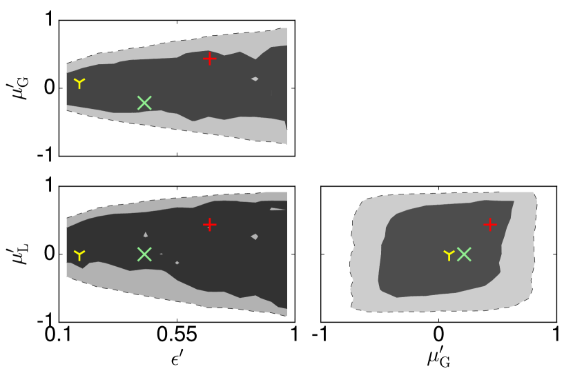
Figure 3: The 68% (dark gray regions) and the 95% CL (light gray regions) 2-dimensional marginalized contours for the generalized Galileon model parameters. The red-plus, green-cross and yellow-triangle points present models for the simplest cubic Galileon, the sDGP and the nDGP models, respectively.

Instead of $\mu_{\rm G}$, $\mu_{\rm L}$ and $\epsilon$, we introduce $\mu_{\rm G}^{\prime}={\mu_{\rm G}}/({1+|\mu_{\rm G}|})$,   $\mu_{\rm L}^{\prime}={\mu_{\rm L}}/({1+|\mu_{\rm L}|})$, and $\epsilon^{\prime}=1-\exp(-\epsilon)$, which span the complete available parameter space of $\mu_{\rm G}^{\prime}$ and $\mu_{\rm L}^{\prime}$ in the interval $[-1,1]$ and $\epsilon^{\prime}$ in the interval $[0,1]$, respectively. General relativity is recovered when $\mu_{\rm G}^{\prime}=\mu_{\rm L}^{\prime}=0$ or $\epsilon^{\prime}\to 1$. Using the same method adopted for Newtonian case, we perform an MCMC analysis for the modified gravity model including $8$ parameters with the chi-squared $\chi^{2}_{\rm BX+SZ+WL}$, defined by (3.1).

Figure 5 shows the 2-dimensional marginalized contours of the different combinations between the model parameters. The best-fit parameters and their 1-dimensional marginalized 68% errors are listed in the Table. 1. The red curve in each panel of figure 1 shows the best-fit profile for the generalized Galileon model with the minimum value of the chi-squared/d.o.f., $\chi^{2}_{\rm XB+SZ+WL}/{\rm d.o.f.}=57/41$. These profiles almost overlap with the profiles for Newtonian gravity (black dashed curves), which shows that the large deviation from Newtonian gravity is rejected. We note that there is no significant difference between the red and black curves in the best-fit profiles. There is a slight difference in the shear profiles at the large radius $r>1$Mpc, which seems to be originated from the large errorbars of the shear data.

Figure 3 shows 2-dimensional marginalized contours of the confidence levels for the parameters $\mu_{\rm G}^{\prime}$, $\mu_{\rm L}^{\prime}$ and $\epsilon^{\prime}$. $\mu_{\rm G}^{\prime}$ and $\mu_{\rm L}^{\prime}$ are parameters from the modification of the gravitational potential and the lensing potential, and $\epsilon^{\prime}$ is a parameter characterizing the Vainshtein radius. Large values of $\mu_{\rm G}$ and $\mu_{\rm L}$ are rejected at the $68\%$ confidence level, which indicates that the possibility of a large deviation from the Newtonian gravity is ruled out, depending on the parameter $\epsilon$. When $\epsilon$ is smaller, the Vainshtein radius becomes smaller, we can put a tighter constraint on $\mu_{\rm G}$ and $\mu_{\rm L}$. However, $\epsilon$ is large, the Vainshtein radius becomes large, which makes difficult to distinguish between the Newtonian gravity model and the modified gravity model due to the Vainshtein mechanism. The red-plus, green-cross and yellow-triangle points in figure 3 show the representative models, the simplest cubic Galileon model, the sDGP model and nDGP model, respectively, at the redshift $z=0.0236$. The parameter values for each models are shown in Table 2.

In a previous work [29], a constraint only on the parameter space $\mu_{\rm L}$ and $\epsilon$ is obtained, based on the lensing observations. As a other recent related work, Barreira et al. investigated cluster masses and the concentration parameters in modified gravity models from shear profiles [62]. They focused their investigation on the mass-concentration relation of 19 X-ray selected clusters from the CLASH survey in the simplest cubic Galileon and Nonlocal gravity models. They found that the mass-concentration relation obtaining from the shear profiles for the cubic Galileon model is the same as those for the $\Lambda$CDM model, but no stringent constraint on the modified gravity models is obtained. Unfortunately the constraint obtained in the present paper is not very stringent too, but one can find the following possibility. We emphasize that models with $\mu_{\rm L}=0$ like the sDGP and the nDGP models are indistinguishable with Newtonian gravity in the method based on the lensing observations. On the other hand, our method of combining the gas and weak-lensing profiles can solve the problem from this degeneracy. Future observations would improve the constraint.

Table 2: Values of modified gravity parameters for each model at the redshift $z=0.0236$.

Models	$\epsilon~{}(\epsilon^{\prime})$	$\mu_{\rm G}~{}(\mu_{\rm G}^{\prime})$	$\mu_{\rm L}~{}(\mu_{\rm L}^{\prime})$
simplest cubic Galileon	${0.77~{}(0.44)}$	${0.77~{}(0.44)}$	${1.12~{}(0.67)}$
sDGP	${-0.26~{}(-0.22)}$	${0~{}(0)}$	${0.53~{}(0.43)}$
nDGP	${0.20~{}(0.18)}$	${0~{}(0)}$	${0.10~{}(0.09)}$

Table 3: Same as Table 1 but for the results of the generalized Galileon model in the unscreened limit with only fixing $\epsilon=0$ (second column), and the case with fixing all the modified gravity parameters $\epsilon^{\prime}=0.05$, $\mu_{\rm G}^{\prime}=0.2$, and $\mu_{\rm L}^{\prime}=0$ (third column).

Parameter	Modified gravity (unscreened)	Modified gravity (fifth force)
$M_{\rm vir}$	${1.26}^{+0.15}_{-3.85}\times 10^{15}~{}M_{\odot}$	${0.86}^{+0.05}_{-0.05}\times 10^{15}~{}M_{\odot}$
$c$	${3.78}^{+0.13}_{-0.55}$	${3.84}^{+0.24}_{-0.28}$
$n_{0}$	${6.15}^{+0.27}_{-0.29}\times 10^{-3}{\rm/cm^{3}}$	${6.20}^{+0.27}_{-0.32}\times 10^{-3}{\rm/cm^{3}}$
$T_{0}$	${6.35}^{+0.13}_{-0.11}~{}{\rm keV}$	${6.36}^{+0.12}_{-0.12}~{}{\rm keV}$
$b_{1}$	${2.6}$ (fixed)	${2.6}$ (fixed)
$b_{2}$	${0.5}$ (fixed)	${0.5}$ (fixed)
$r_{1}$	${0.75}^{+0.06}_{-0.07}~{}{\rm Mpc}$	${0.75}^{+0.06}_{-0.06}~{}{\rm Mpc}$
$\epsilon^{\prime}$	${0}$ (fixed)	${0.05}$ (fixed)
$\mu_{\rm G}^{\prime}$	${-0.10}$	${0.2}$ (fixed)
$\mu_{\rm L}^{\prime}$	${-0.05}$	${0}$ (fixed)
Minimum $\chi^{2}$/d.o.f.	${57/42}$	${60/44}$

5 Discussion

5.1 Degeneracies on parameters

On the MCMC analysis in the previous section, we do not take the range of $\epsilon$, $[0,0.1]$, into account because it is hard to converge the MCMC runs because of degeneracy in the parameter space. Here, we treat this parameter region for complemental discussion.

First, taking the limit $\epsilon\to 0$, which means the fifth force is unscreened everywhere, the solutions of the gas pressure (4.10) and the convergence (4.11) are reduced to

$$P_{\rm e}(r)=P_{0}\exp\left(\int_{0}^{r}dr\frac{\mu m_{\rm p}}{kT_{\rm e}(r)}\left[-\frac{GM(<r)}{r^{2}}(1+\mu_{\rm G})\right]\right),$$ (5.1)

$$\kappa(r_{\perp})=(1+\mu_{\rm L})\frac{2}{\Sigma_{\rm c}}\int_{0}^{\infty}dz\rho(r).$$ (5.2)

Then, the pressure profile and the convergence profile are simply modified by a factor of $(1+\mu_{\rm G})$ and $(1+\mu_{\rm L})$, respectively. In this case, we have $P_{\rm e}\propto(1+\mu_{\rm G})M_{\rm vir}m(c)/c^{3}$ and $\kappa\propto\rho_{\rm s}\propto(1+\mu_{\rm L})M_{\rm vir}c^{3}/m(c)$, then, there are degeneracies between the parameters, $M_{\rm vir},c,\mu_{\rm G}$, and $\mu_{\rm L}$. Figure 6 compares the results of the MCMC analysis with fixing $\epsilon=0$ (dark blue region ($68$% CL) and mid blue region ($95$% CL)) and the results of the Newtonian gravity (dark gray region and mid gray region), which is the same as those of figure 4. The best-fit parameters are shown in the Table. 3. The CL contours of the blue regions reflect the degeneracy between the parameters, $M_{\rm vir},c,\mu_{\rm G}$, and $\mu_{\rm L}$.

Next, we show how the presence of the fifth force affects the parameter estimation. For example, the blue confidence contours in figure 7 shows the $68$% and $95$% confidence contours of the case with fixing $\epsilon=0.05$, $\mu_{\rm G}=0.2$ and $\mu_{\rm L}=0$. $M_{\rm vir}$ and $c$ are different from those of the Newtonian gravity (gray regions), but other parameters, $n_{0}$, $T_{0}$ and $b_{1}$, are not changed. The minimum value of the chi-squared/d.o.f. in the presence of the fifth force is $\chi^{2}_{\rm XB+SZ+WL}/{\rm d.o.f.}=60/44$, which is almost the same as the Newtonian case, despite the different cluster parameter, $M_{\rm vir}\sim 0.9\times 10^{15}M_{\odot}$ (see Table. 3). This result exemplifies that the presence of the attractive fifth force affects the estimation of the NFW parameters, $M_{\rm vir}$ and $c$. This is understood as the consequence of the degeneracy between the modification parameters $\mu_{\rm G}$ and $\mu_{\rm L}$ and $M_{\rm vir}$ and $c$.

5.2 Systematic errors

We shall discuss possible systematic errors. In our analysis, we have assumed spherical symmetry for the matter distribution and an equilibrium state for the gas component of the balance between the pressure gradient and the gravitational force and the fifth force in the case of its presence. We have demonstrated that non-thermal pressure at the level suggested by numerical simulations does not alter our results. A future X-ray satellite, ASTRO-H [63], will observe turbulent gas motion in the Coma Cluster in more detail, which will be informative regarding our result. However, observations of the Coma Cluster suggest substructures [49, 34, 64, 65, 66, 67] and orientation dependence [40, 41, 47], so the Coma Cluster is not thought to be a relaxed system. Dynamical states of the Coma Cluster would give a systematic difference between our results and temperature measurement. Our fitting results show that the temperature of the Coma Cluster is around $6.4$ keV (see Table. 1), but this result seems lower than those of X-ray observations [32, 33, 40, 41, 45, 46, 47], which estimate that the temperature of the Coma Cluster is around $8$–$9$ keV. Comparing the mass-temperature scaling relation for a sample of relaxed clusters [68] with an X-ray temperature observation of the Coma Cluster [32, 33], the observed temperature is higher that the temperature expected by the mass. The enhancement is at 3$\sigma$ level of intrinsic scatter [68]. Similar results of high temperatures have also been reported by a comparison with other clusters [69]. Depending on the orientation and excluding the central region, the temperature of the Coma Cluster could be around $6$–$7$ keV [32, 40], but it is difficult to take this dependence into account. Therefore, systematic error of temperature in the Coma Cluster would cause a substantial influence to the proposed fitting method. In order to reduce a possible dependence of cluster-dynamical states and halo triaxiality, it is of vital importance to increase the number of sampling clusters. Ongoing and future multi-wavelength surveys such as the Hyper Suprime-Cam (HSC) optical survey, the Dark Energy Survey (DES) [70], the eROSITA X-ray survey [71], and the ACT-Pol [72] and SPT surveys [73] will be powerful aids to better constraining the gravity model.

6 Summary and Conclusion

In this paper, we obtained a constraint on the generalized Galileon model through the Coma Cluster observations of X-ray brightness, the SZ effect and weak lensing. We have constructed a simple analytic model of the gas distribution profiles and the weak-lensing profile (c.f. [27, 28, 29]). The fifth force affects not only the gas distribution but also the weak-lensing profile. In general, the effects depend on different parameters characterizing the generalized Galileon model. These features can be investigated by combination of the observations of a galaxy cluster reflecting the gas density profile and the lensing signals. Their multi-wavelength observations are complementary to each other, and are useful to put a constraint on the modified gravity model by breaking the degeneracy between the model parameters. Systematic study compiling multi-wavelength datasets for a large number of clusters enables us to well reduce the systematic errors and constraints on the modified gravity models. However, the degeneracy between the parameters, $M_{\rm vir}$, $c$, $\mu_{\rm G}$ and $\mu_{\rm L}$, persists in the limit of the weak screening of the fifth force, which affects the estimation of the cluster parameters. Future and ongoing surveys and their joint analysis would be a powerful aid to obtaining a more stringent constraint on modified gravity models.

Appendix A Definitions of the coefficients

In this appendix, we summarize the coefficients between the generalized Galileon model and the specific models used in section 4 (see also [29, 74]). The coefficients in the perturbation equations (4.2)–(4.4) are defined as

$$\alpha =\alpha_{1},$$ (A.1)

$$\xi =\alpha_{2},$$ (A.2)

$$\zeta =\frac{4(\alpha_{1}+\alpha_{2})}{\beta}\frac{G_{4}H}{\dot{\phi}\phi},$$ (A.3)

$$\lambda^{2} =\frac{2\beta_{0}G_{4}\phi H}{\beta X\dot{\phi}},$$ (A.4)

$$\beta =-4(\alpha_{0}+2\alpha_{1}\alpha_{2}+\alpha_{2}^{2})\frac{G_{4}H^{2}}{\dot{\phi}^{2}},$$ (A.5)

where

$$\alpha_{0} =\left(\frac{\dot{\Theta}}{H^{2}}+\frac{\Theta}{H}-2G_{4}-4\frac{\dot{G}_{4}}{H}-\frac{{\cal E+P}}{2H^{2}}\right){1\over 2G_{4}},$$ (A.6)

$$\alpha_{1} =\left(2\frac{\dot{\phi}G_{4\phi}}{H}\right){1\over 2G_{4}},$$ (A.7)

$$\alpha_{2} =\left(\frac{\dot{\phi}XG_{3X}}{H}-\frac{\dot{\phi}G_{4\phi}}{H}\right){1\over 2G_{4}},$$ (A.8)

$$\beta_{0} =\left(\frac{\dot{\phi}XG_{3X}}{H}\right){1\over 2G_{4}},$$ (A.9)

$$\Theta =-\dot{\phi}XG_{3X}+2HG_{4}+\dot{\phi}G_{4\phi}.$$ (A.10)

These coefficients are determined by the background solution, which follows:

$$2XK_{X}-K+6X\dot{\phi}HG_{3X}-2XG_{3\phi}-6H^{2}G_{4}-6H\dot{\phi}G_{\phi}=\rho_{\rm m},$$ (A.11)

$$K-2X\left(G_{3\phi}+\ddot{\phi}G_{3X}\right)+2\left(3H^{2}+2\dot{H}\right)G_{4}+2\left(\ddot{\phi}+2H\dot{\phi}\right)G_{4\phi}+4XG_{4\phi\phi}=0,$$ (A.12)

where $\rho_{\rm m}$ is the non-relativistic matter energy density and $H=\dot{a}/a$ is the Hubble parameter. The background equation for the scalar field is written as

$$\dot{J}+3HJ-P=0,$$ (A.13)

with

$$J \equiv\dot{\phi}K_{X}+6HXG_{3X}-2\dot{\phi}G_{3\phi},$$ (A.14)

$$P \equiv K_{\phi}-2X\left(G_{3\phi\phi}+\ddot{\phi}G_{3\phi X}\right)+6\left(2H^{2}+\dot{H}\right)G_{4\phi}.$$ (A.15)

The simplest cubic Galileon model is defined by $G_{4}=M_{\rm Pl}^{2}/2$, $K=-X$ and $G_{3}=(r_{\rm c}^{2}/M_{\rm Pl})X$, which corresponds to taking $c_{1}=-1$ in Ref. [75], and thus the coefficients in the perturbation equations are

$$\alpha =0,$$ (A.16)

$$\xi =4\pi G_{3}G_{3X}\dot{\phi}^{2}\phi,$$ (A.17)

$$\zeta =\frac{G_{3X}\dot{\phi}^{2}}{\beta\phi},$$ (A.18)

$$\lambda^{2} =\frac{G_{3X}\phi}{\beta},$$ (A.19)

$$\beta =-1+2G_{3X}(\ddot{\phi}+2H\dot{\phi})-4\pi G_{3}G_{3X}^{2}\dot{\phi}^{4}.$$ (A.20)

When we adopt the late time de Sitter attractor solution [76],

$$\left(\frac{H(a)}{H_{0}}\right)^{2}=\frac{1}{2}\left[\frac{\Omega_{\rm m0}}{a^{3}}+\sqrt{\left(\frac{\Omega_{\rm m0}}{a^{3}}\right)^{2}+4(1-\Omega_{\rm m0})}\right].$$ (A.21)

The combinations $\xi\zeta$ and $\lambda^{2}\zeta$ are given by

$$\xi\zeta =\frac{(1-\Omega_{\rm m})(2-\Omega_{\rm m})}{\Omega_{\rm m}(5-\Omega_{\rm m})},$$ (A.22)

$$\lambda^{2}\zeta =\left(\frac{2-\Omega_{\rm m}}{H\Omega_{\rm m}(5-\Omega_{\rm m})}\right)^{2},$$ (A.23)

where $\Omega_{\rm m}(a)=\rho_{\rm m}(a)/3M_{\rm Pl}^{2}H^{2}(a)$ is the matter density parameter.

Within the sub-horizon approximation, the DGP model [18, 19, 22] can be effectively described by the coefficients

$$\alpha =-1,$$ (A.24)

$$\xi =\frac{1}{2},$$ (A.25)

$$\zeta =-\frac{2}{3\beta},$$ (A.26)

$$\lambda^{2} =-\frac{r_{\rm c}^{2}}{3\beta},$$ (A.27)

$$\beta =1\pm 2Hr_{\rm c}\left(1+\frac{\dot{H}}{3H^{2}}\right),$$ (A.28)

where the sign “$\pm$” in $\beta$ represents the case of the sDGP model with “$-$” sign and the nDGP model with “$+$” sign. For the sDGP model, we adopt the self-accelerating background solution, which is specified by the modified Friedmann equation in the sDGP model [21],

$$\frac{H(a)}{H_{0}}=\frac{1-\Omega_{\rm m0}}{2}+\sqrt{\frac{\Omega_{\rm m0}}{a^{3}}+\frac{(1-\Omega_{\rm m0})^{2}}{4}},$$ (A.29)

and $r_{\rm c}=1/(1-\Omega_{\rm m0})H_{0}$. On the other hand, the nDGP model has no self-accelerating solution without introducing the cosmological constant [11, 13]. Here we consider the nDGP model with introducing a dynamical dark energy component on the brane, which is tuned such that the background evolves as in the lambda cold dark matter model [77].

Figure 4: The 68% (dark gray region) and the 95% CL (mid gray region) 2-dimensional marginalized contours for the 5 model parameters, $M_{\rm vir}~{}[10^{14}M_{\odot}]$, $c$, $n_{0}~{}[10^{-3}{\rm cm}^{-3}]$, $T_{0}~{}[{\rm keV}]$ and $r_{1}~{}[{\rm Mpc}]$. The rightmost plots of each row show the 1-dimensional marginalized constraints (solid) and likelihood distributions (dotted).

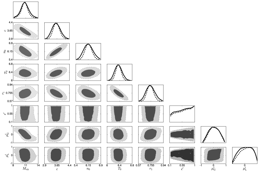
Figure 5: Same as figure 4 but when including the modification parameters $\epsilon^{\prime}$, $\mu_{\rm G}^{\prime}$ and $\mu_{\rm L}^{\prime}$ in the MCMC analysis.

Figure 6: The dark blue region ($68$% CL) and the mid blue region ($95$% CL) are the results of the MCMC analysis for the modified gravity model with fixing $\epsilon=0$. The dark gray region ($68$% CL) and the mid gray region ($95$% CL) are the results for the Newtonian gravity (same as the figure 4).

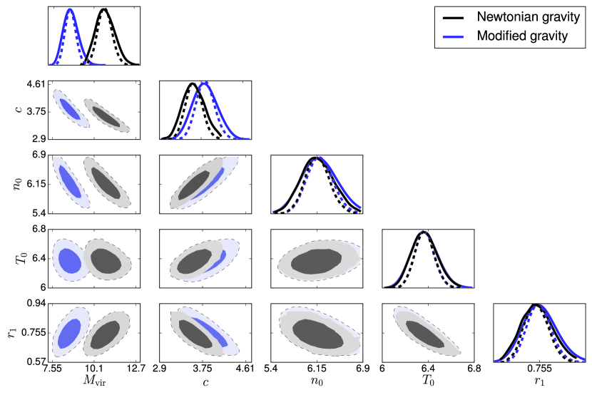
Figure 7: The dark blue region ($68$% CL) and the mid blue region ($95$% CL) are the results of the MCMC analysis for the modified gravity model with fixing $\epsilon^{\prime}=0.05$, $\mu_{\rm G}^{\prime}=0.2$ and $\mu_{\rm L}^{\prime}=0$. The dark gray region ($68$% CL) and the mid gray region ($95$% CL) are the results for the Newtonian gravity (same as the figure 4).

References

- [1] E. G. Adelberger, B. R. Heckel, and A. E. Nelson, Annu. Rev. Nucl. Part. Sci. 53 (2003) 77.
- [2] C. M. Will, Living Rev. Relativity 17 (2014) 4; arXiv:1403.7377.
- [3] J. Khoury, A. Weltman, Phys. Rev. D 69 (2004) 044026.
- [4] D. F. Mota, J. D. Barrow, Phys. Lett. B 581 (2004) 141.
- [5] A.A. Starobinsky, JETP Lett. 86 (2007) 157.
- [6] W. Hu and I. Sawicki, Phys. Rev. D 76 (2007) 064004.
- [7] S. Tsujikawa, Phys. Rev. D 77 (2008) 023507.
- [8] L. Lombriser, Annalen der Physik 526 (2014) 259; arXiv:1403.4268.
- [9] A. I. Vainshtein, Phys. Lett. B 39 (1972) 393.
- [10] G. R. Dvali, G. Gabadadze and M. Porrati, Phys. Lett. B 485 (2000) 208.
- [11] C. Deffayet, Phys. Lett. B 502 (2001) 199.
- [12] A. Nicolis, R. Rattazzi and E. Trincherini, Phys. Rev. D 79 (2009) 064036.
- [13] C. Deffayet, G. Esposito-Farese and A. Vikman, Phys. Rev. D 79 (2009) 084003.
- [14] C. Deffayet, G. R. Dvali and G. Gabadadze, Phys. Rev. D 65 (2002) 044023.
- [15] M. A. Luty, M. Porrati and R. Rattazzi, J. High Energy Phys. 0309 (2003) 029.
- [16] T. Kobayashi, M. Yamaguchi and J. Yokoyama, Phys. Rev. Lett. 105 (2010) 231302.
- [17] R. Kimura, T. Kobayashi and K. Yamamoto, Phys. Rev. D 85 (2a012) 024023.
- [18] K. Koyama and Maartens, JCAP 01 (2006) 016.
- [19] K. Koyama and F. P. Silva, Phys. Rev. D 75 (2007) 084040.
- [20] F. Schmidt, Phys. Rev. D 80 (2009) 043001; arXiv:0905.0858.
- [21] D. Deffayet, G. R. Dvali and G. Gabadadze, Phys. Rev. D 65 (2002) 044023.
- [22] B. Falck, K. Koyama and Gong-Bo Zhao arXiv:1503.06673.
- [23] F. Schmidt, Phys. Rev. D 80 (2009) 123003; arXiv:0910.0235.
- [24] A. Nicolis and R. Rattazzi, JHEP 06 (2004) 059; arXiv:hep-th/0404159.
- [25] D. Goubnov, K. Koyama and S. Sibiryakov, Pys. Rev. D 73 (2006) 044016.
- [26] A. Terukina and K. Yamamoto, Phys. Rev. D 86 (2012) 103503.
- [27] A. Terukina, L. Lombriser, K. Yamamoto, D. Bacon, K. Koyama and R.C. Nichol, JCAP 04 (2014) 013.
- [28] H. Wilcox, et al., arXiv:1504.03937 [Mon. Not. Roy. Astron. Soc. (to be published)].
- [29] T. Narikawa, K. Yamamoto, JCAP 05 (2013) 016.
- [30] T. Narikawa, T. Kobayashi, D, Yamauchi and Ryo Saito, Phys. Rev. D 87 (2013) 124006.
- [31] R.A. Sunyaev and Y. Zel’dovich, Space. Sci. 7 (1970) 3.
- [32] K. Matsushita, Astron. Astrophys. 527 (2011) A134; arXiv:1101.1849.
- [33] K. Matsushita T. Sato, E. Sakuma and K. Sato, Publ. Astron. Soc. Jpn. 65 (2013) 10; arXiv:1208.6098.
- [34] N. Okabe, T. Futamase, M. Kajisawa and R. Kuroshima, Astrophys. J. 784 (2014) 27; arXiv:1304.2399.
- [35] J. F. Navarro, C. S. Frenk and S. D. M. White, Astrophys. J. 490 (1997) 493.
- [36] T.T. Nakamura and Y. Suto, Prog. Theor. Phys. 97 (1997) 49; astro-ph/9612074
- [37] K.A. Arnaud, The First Ten Years Astronomical Data Analysis Software and Systems V, eds. G. Jacoby and J. Barnes, ASP Conf. Series volume 101 (1996) 17 [http://heasarc.gsfc.nasa.gov/docs/xanadu/xspec/index.html].
- [38] R.K. Smith, N.S. Brickhouse, D.A. Liedahl and J.C. Raymond, Astrophys. J. 556 (2001) L91.
- [39] C. Oaxaca Wright and T. G. Brainerd, arXiv:astro-ph/9908213.
- [40] A. Simionescu et al., arXiv:1302.4140.
- [41] T. Sato et al., Publ. Astron. Soc. Jpn. 63 (2011) 991; arXiv:1109.0154.
- [42] D.M. Neumann, D.H. Lumb, G.W. Pratt and U.G. Briel, Astron. Astrophys. 400 (2003) 811; arXiv:astro-ph/0212432.
- [43] J. S. Sanders et al., Science 341 (2013) 6152; arXiv:1309.4866.
- [44] F. Churazov et al., Mon. Not. Roy. Astron. Soc. 421 (2012) 1123.
- [45] S.L. Snowden, R.F. Mushotzky, K.D. Kuntz and D.S. Davis, Astron. Astrophys. 478 (2008) 615.
- [46] D.R. Wik et al., Astrophys. J. 696 (2009) 1700.
- [47] F. Gastaldello, et al., Astrophys. J. 800 (2015) 139.
- [48] Planck Collaboration: P. A. R. Ade et al., Astron. Astrophys. 554 (2013) A140; arXiv:1208.3611.
- [49] N. Okabe, Y. Okura and T. Futamase, Astrophys. J. 713 (2010) 291.
- [50] B. Audren, J. Lesgourgues, K. Benabed and S. Prunet, JCAP 02 (2013) 001; arXiv:1210.7183.
- [51] N. Metropolis et al., J. Chem. Phys. 21 (1953) 1087.
- [52] W.K. Hastings, Biometrika 57 (1970) 97.
- [53] A. Gelman and Rubin, Statist. Sci. 7 (1992) 457.
- [54] P. Schuecker et al., Astron. Astrophys. 426 (2004) 387.
- [55] L. D. Shaw et al., ApJ. 725, 1452 (2010)
- [56] N. Battaglia, J.R. Bond, C. Pfrommer and J.L. Sievers, Astrophys. J. 758 (2012) 74; arXiv:1109.3709.
- [57] A. De Felice, R. Kase, S. Tsujikawa, Phys. Rev. D 85 (2012) 044059.
- [58] R. Kimura and K. Yamamoto, JCAP 04 (2011) 025.
- [59] G.W. Horndeski Int. J. Theor. Phys. 10 (1974) 363.
- [60] C. Deffayet, X. Gao, D.A. Steer and G. Zahariada, Phys. Rev. D 80 (2011) 064039; arXiv:1103.3260.
- [61] T. Kobayashi, M. Yamaguchi and J. Yokoyama, Prog. Theor. Phys. 129 (2011) 3; arXiv:1105.5723.
- [62] A. Barreira, et al., arXiv:1505.03468.
- [63] T. Kitayama, et al., arXiv:1412.1176 [http://astro-h.isas.jaxa.jp/en].
- [64] H. Honda et al., Astrophys. J. 473 (1996) L71.
- [65] M. Watanabe et al., Astrophys. J. 527 (1999) 80.
- [66] M. Arnaud et al., Astron. Astrophys. 365 (2001) L67;arXiv:astro-ph/0011086.
- [67] D.M. Neumann, D.H. Lumb, G.W. Pratt and U.G. Briel, Astron. Astrophys. 400 (2003) 811; arXiv:astro-ph/0212432.
- [68] N. Okabe et al., Publ. Astron. Soc. Jpn. 66 (2014) 99; arXiv:1406.3451.
- [69] K.A. Pimbblet, S.J. Penny and R.L. Davies Mon. Not. Roy. Astron. Soc. 438 (2014) 3049; arXiv:1312.3698.
- [70] The Dark Energy Survey Collaboration, arXiv:astro-ph/0510346 [http://www.darkenergysurvey.org].
- [71] A. Merloni, et al., arXiv:1209.3114 [http://www.darkenergysurvey.org].
- [72] M.D. Niemack, et al., arXiv:1006.5049 [http://www.princeton.edu/act].
- [73] The SPT Collaboration, Proc. SPIE Int. Soc. Opt. Eng. 5498 (2014) 11; arXiv:astro-ph/0411122 [http://pole.uchicago.edu/index.php].
- [74] T. Narikawa, R. Kimura, T. Yano and K. Yamamoto, Int. J. Mod. Phys. D 20 (2011) 2383.
- [75] A. Barreira, B. Li, C.M. Baugh and S. Pascoli, arXiv:1406.0485.
- [76] S. Nesseris, A. De Felice and S. Tsujikawa, Observational constraints on Galileon cosmology, Phys. Rev. D 82 (2010) 124054.
- [77] F. Schmidt, Phys. Rev. D 80 (2009) 123003; arXiv:0910.0235