Fermionic dark matter and neutrino masses in a $\cal{B}-\cal{L}$ model

Abstract

In this work we present a common framework for neutrino mass and dark matter. Specifically, we work with a local $\mathcal{B-L}$ extension of the standard model which has three right-handed neutrinos, $n_{R_{i}}$, and some extra scalars, $\Phi,\,\phi_{i}$ besides the standard model fields. The $n_{R_{i}}$’s have non-standard $\mathcal{B-L}$ quantum numbers and thus these couple to different scalars. This model has the attractive property that an almost automatic $\mathbb{Z}_{2}$ symmetry acting only on a fermionic field, $n_{R3}$, is present. Taking advantage of this $\mathbb{Z}_{2}$ symmetry, we study both the neutrino mass generation via a natural see-saw mechanism in low energy and the possibility of $n_{R3}$ to be a DM candidate. For this last purpose, we study its relic abundance and its compatibility with the current direct detection experiments.

I introduction

At least two experimental evidences demand for physics beyond the standard model (SM). The first one comes from the well stablished neutrino oscillation experiments (SuperK, ; SNO, ; KamLAND, ; MINOS, ) which imply that all the three known neutrinos ($\nu_{e},\,\nu_{\mu},\,\nu_{\tau}$) are quantum superpositions of three massive states $\nu_{i}$ ($i=1,\,2,\,3$). The second evidence is firmly stablished from several observations and studies of gravitational effects on different scales, which points out that most of the Universe’s mass consists of non-baryonic dark matter (DM). Specifically, the Planck collaboration has determined that the DM relic abundance is given $\Omega_{\text{DM}}h^{2}=0.1193\pm 0.0014$ (PLANCK_2013, ).

In order to explain both of these evidences, it is now clear that the SM has to be extended. In the neutrino case, usually new fermionic fields, $n_{R}$’s, are introduced to generate Dirac mass terms for neutrinos. The $n_{R}$ fields are, in general, singlet under the SM gauge groups, and thus these can also have Majorana mass terms. Moreover, in order to explain the smallness of active neutrino masses, the $n_{R}$’s usually get large masses via the well known see-saw mechanism (KingLuhn:2013neutrinomixing, ; see-saw_Gonzalez_Garcia, ). On the other hand, the existence of DM in the Universe requires at least a new massive particle since SM does not provide any viable DM candidate. The most studied and well motivated candidates for DM are the weakly interacting massive particles (WIMPs). In general, WIMPs are neutral, stable and are present in a plethora of extensions of the SM (WIMPS1, ; WIMPS2, ; WIMPS3, ; WIMPS4, ). Nowadays, there are several astroparticle experiments actively pursuing detection of WIMP DM candidates in direct and indirect ways. The direct detection experiments (LUX_2014, ; XENON100_2012, ; SuperCDMS_2014, ) have set upper bounds on WIMP-nucleon elastic scattering, whereas the indirect ones (ID1, ; ID2, ; ID3, ; ID4, ; ID5, ) presented upper limits on the thermal average of the same scattering cross section $\left\langle\sigma v_{\textrm{Mol}}\right\rangle$.

In this work we study a scenario that simultaneously offers an explanation for the previously mentioned open questions of the SM. In special, we present a local $\mathcal{B-L}$ extension of the SM in which there are three $n_{R}$ fermionic fields and some extra scalars, $\Phi,\,\phi_{i}$. The $\mathcal{B-L}$ quantum numbers of the extra new fermionic fields come from exotic solutions of anomaly constraints. These solutions were found for the first time in Ref. (Montero:2007cd, ). Here, we propose a simplified version of the model in Ref. (Montero:2007cd, ; Bruce:2011Neutrinos, ) where an almost natural $\mathbb{Z}_{2}$ symmetry stabilizes $n_{R_{3}}$ and thus allows it to be a DM candidate. Another appealing feature of this model is that it implements a see-saw mechanism at low energy because neutrino masses are proportional to $V_{\Phi}^{2}/V_{\phi}$ (where $V_{\Phi}$ and $V_{\phi}$ are VEVs of the $\Phi,$ $\phi_{i}$, respectively) and $V_{\Phi}$ has been set in MeV energy scale. The discrete symmetry also simplifies the task of setting the Yukawa couplings in the neutrino mass Lagrangian in order to agree with the neutrino oscillation parameters. There have been extensive studies on these two matters, in special in gauge extensions of the SM (a few of which are contained in the Refs. (Bruce:2014DM, ; DM_with_neutrinos1, ; DM_with_neutrinos2, )). This is so because U$(1)$ gauge factors are contained in grand unification theories (GUT1, ; GUT2, ), supersymmetric models (SUSY_add_1, ) and left-right models (left_right_1, ; left_right_2, ).

The paper is organized as follows. We start by discussing the model in Sec. II. In that section we present its field content and general Lagrangian. We also show the almost natural $\mathbb{Z}_{2}$ symmetry in the model which stabilizes the DM candidate $n_{3R}$. In Sec. III we study the scalar sector in detail. We obtain analytical formulas for both the mass eigenstates and the eigenvalues when it is possible. We also include a discussion about the consequences of the presence of the Majoron $J$ which is due to the breaking of an accidental global U$(1)_{J}$ symmetry. Specifically, we show that it escapes the current bounds on energy loss in stars (geJ_stars1, ; geJ_stars2, ), effective number of neutrinos $N_{\textrm{eff}}$ (PLANCK_2013, ), and the invisible decay widths of Higgs (Ellis_2013, ; Giardino2014, ; Atlascollaboration, ; CMScollaboration, ) and $Z_{1}$ gauge boson. In Sec. IV we analytically find the parameters of the neutrino mass matrices in order to satisfy the data from the neutrino oscillation (Olive:2014PDG, ) and other constraints such as lepton flavor violation (LFV) (mee_future, ; mee_CUORE_2015, ); the sum of the SM neutrinos masses (PLANCK_2013, ); and effective Majorana mass $m_{ee}$ from double beta decay experiments (mee_future, ; mee_CUORE_2015, ). In Sec. V we carry out a study of the relic dark matter abundance and the direct detection prospects. A general discussion follows in Sec. VI where we present our conclusions. Finally, in Appendix A we show the general minimization conditions coming from the scalar potential.

II the model

We consider an extension of the SM based on the gauge symmetry SU$(2)_{L}\otimes$U$(1)_{Y^{{}^{\prime}}}\otimes$U$(1)_{\cal{B}-\cal{L}}$ where $\cal{B}$ and $\cal{L}$ are the usual baryonic and leptonic numbers, respectively, and $Y^{\prime}$ is a new charge different from the hypercharge $Y$ of the SM. The values of $Y^{\prime}$ are chosen to obtain the hypercharge $Y$ through the relation $Y=[Y^{\prime}+{\cal{B}-{\cal{L}}}]$, after the first spontaneous symmetry breaking. The fields of this model with their respective charges are shown in Table 1. Actually, this model is a simplified variation of the one introduced in Refs. (Montero:2007cd, ; Bruce:2011Neutrinos, ). Specifically, here we have removed one of the extra doublets of scalars considered there. As we will show below, this allows an almost automatic $\mathbb{Z}_{2}$ symmetry that stabilizes the DM candidate, $n_{R3}$. The remaining scalar fields are enough to give mass to the neutrinos at tree level. It is also important to note that there is an exotic charge assignment for the ${\cal{B}-{\cal{L}}}$ charges where $({\cal{B}-{\cal{L}}}){}_{n_{R1},n_{R2}}=-4$ and $({\cal{B}-{\cal{L}}}){}_{n_{R3}}=5$ different from the usual one where $({\cal{B}-{\cal{L}}}){}_{n_{Ri}}=1$ with $i=1,\,2,\,3$.

Fermion	$I_{3}$	$Y^{\prime}$	$\cal{B}-\cal{L}$	Scalar	$I_{3}$	$Y^{\prime}$	$\cal{B}-\cal{L}$
$\nu_{eL},\,e_{L}$	$\pm$ 1/2	0	-1	$H^{+,0}$	$\pm$ 1/2	1	0
$e_{R}$	0	-1	-1	$\Phi^{0,-}$	$\pm$ 1/2	-4	3
$u_{L},\,d_{L}$	$\pm$ 1/2	0	1/3	$\phi_{1}$	0	-8	8
$u_{R}$	0	1	1/3	$\phi_{2}$	0	10	-10
$d_{R}$	0	-1	1/3	$\phi_{3}$	0	1	-1
$n_{R1},n_{R2}$	0	4	-4	$\phi_{\textrm{X}}$	0	3	-3
$n_{R3}$	0	-5	5

Table 1: Quantum number assignment for the fields in the model. $I_{3}$, $Y^{\prime}$ and $\cal{B}-\cal{L}$ are the quantum numbers under the symmetry groups SU$(2)_{L}$, U$(1)_{Y^{{}^{\prime}}}$, U$(1)_{\cal{B}-\cal{L}}$, respectively.

With the field content in Table 1, we can write respectively the most general renormalizable Yukawa Lagrangian and scalar potential respecting the gauge invariance as follows

$$-\mathscr{L}_{\text{Y}} = Y_{i}^{(l)}\overline{L}_{Li}e_{Ri}H+Y_{ij}^{(d)}\overline{Q}_{Li}d_{Rj}H+Y_{ij}^{(u)}\overline{Q}_{Li}u_{Rj}\widetilde{H}+\mathcal{D}_{im}\overline{L}_{Li}n_{Rm}\Phi$$ (1)

$$+\frac{1}{2}\mathcal{M}_{mn}\overline{(n_{Rm})^{c}}n_{Rn}\phi_{1}+\frac{1}{2}\mathcal{M}_{33}\overline{(n_{R3})^{c}}n_{R3}\phi_{2}+\frac{1}{2}\mathcal{M}_{m3}\overline{(n_{Rm})^{c}}n_{R3}\phi_{3}+\textrm{H.c.},$$

and

$$V_{{\cal{B}-{\cal{L}}}} = -\mu_{H}^{2}H^{\dagger}H+\lambda_{H}\left|H^{\dagger}H\right|{}^{2}-\mu_{\Phi}^{2}\Phi^{\dagger}\Phi+\lambda_{\Phi}\left|\Phi^{\dagger}\Phi\right|^{2}-\mu_{\alpha}^{2}\left|\phi_{\alpha}\right|^{2}+\lambda_{\alpha}\left|\phi_{\alpha}^{\ast}\phi_{\alpha}\right|^{2}$$ (2)

$$+\kappa_{H\Phi}\left|H\right|^{2}\left|\Phi\right|^{2}+\kappa_{H\Phi}^{\prime}(H^{\dagger}\Phi)(\Phi^{\dagger}H)+\kappa_{H\alpha}\left|H\right|^{2}\left|\phi_{\alpha}\right|^{2}+\kappa_{\Phi\alpha}\left|\Phi\right|^{2}\left|\phi_{\alpha}\right|^{2}$$

$$+\kappa_{\alpha\beta}(\phi_{\alpha}^{\ast}\phi_{\alpha})(\phi_{\beta}^{\ast}\phi_{\beta})+\left[\kappa_{123}\phi_{1}\phi_{2}(\phi_{3}^{\ast})^{2}-i\kappa_{H\Phi X}\Phi^{T}\tau_{2}H\phi_{X}+\kappa_{123X}(\phi_{X}^{\ast}\phi_{1})(\phi_{2}\phi_{3})\right.$$

$$\left.+\kappa^{\prime}_{3X}(\phi_{X}^{\ast}\phi_{3}^{3})+\textrm{H.c.}\right],$$

where $i,j=1,2,3$ are lepton/quark family numbers; $m,n=1,2$; $\widetilde{H}=i\tau_{2}H^{\ast}$ ($\tau_{2}$ is the Pauli matrix), and $\alpha,\beta=1,2,3,X$ with $\alpha\neq\beta$ in the $\kappa_{\alpha\beta}(\phi_{\alpha}^{\ast}\phi_{\alpha})(\phi_{\beta}^{\ast}\phi_{\beta})$ terms. Also, we have omitted summation symbols over repeated indices.

Before we go further, two important remarks are in order. Firstly, from Eqs. (1) and (2) we see that apart from the $\frac{1}{2}\mathcal{M}_{m3}\overline{(n_{Rm})^{c}}n_{R3}\phi_{3}+\textrm{H.c.}$ terms, the Lagrangian is invariant under a $\mathbb{Z}_{2}$ symmetry acting in a non-trivial way on the $n_{R3}$ field, i.e. $\mathbb{Z}_{2}(n_{R3})=-n_{R3}$ (the rest of fields being invariant under this symmetry). We will consider the case of this $\mathbb{Z}_{2}$ symmetry throughout this work. Hence, the $n_{R3}$ fermionic field will be the DM candidate. Secondly, from Eq. (1) we see that quarks and charged leptons obtain masses just from the $H$ vacuum expectation value, $\left\langle H^{0}\right\rangle\equiv V_{H}$. Therefore, the $H$ interactions with quarks and charged leptons are diagonalized by the same matrices as the corresponding mass matrices. In this case the neutral interactions are diagonal in flavor and there is no flavor-changing neutral current in the quark and charged lepton sector. This feature remains after the symmetry basis is changed to mass basis (Glashow1958, ; Cheng1987, ). However, lepton flavor violation (LFV) processes coming from the terms proportional to $\mathcal{D}_{im}$ and $\mathcal{D}_{i3}$ can occur at one loop. We will discuss these processes in more detail in Sec. IV.

III scalar sector

In the general case this model has a rich scalar spectrum and its vacuum structure can take several configurations. However, we are going to make some simplifying and reasonable assumptions that allow us, in most cases, to obtain analytical formulas in both the neutrino and the dark matter sectors. We will discuss systematically our assumptions throughout this paper.

Firstly, as result of the absence of one of the extra doublets and of writing only the renormalizable terms in the scalar potential, the model here considered has a Majoron, $J$, in its scalar spectrum. This is a general conclusion and does not depend on any particular choice of the set of parameters. Once the neutral scalars develop non-vanishing vacuum expectation values, VEVs, and using the usual shifting $\varphi^{0}=\frac{1}{\sqrt{2}}\left(V_{\varphi}+\textrm{Re}\,\varphi+i\,\textrm{Im}\,\varphi\right)$ for the scalar fields (the superscript “$0$” means we are taking the neutral part of the field), we find that $J$ can be written as

$$J = \frac{1}{N_{J}}\left[-9\sqrt{2}V_{H}V_{\phi}^{3}\epsilon^{2}\,\textrm{Im}\,H^{0}-9\sqrt{2}V_{H}^{2}V_{\phi}^{2}\epsilon\,\textrm{Im}\,\Phi^{0}\right.$$ (3)

$$\left.+\frac{1}{\sqrt{2}}V_{\phi}^{2}\left(10V_{H}^{2}+\left(3V_{H}^{2}+10V_{\phi}^{2}\right)\epsilon^{2}\right)\,\textrm{Im}\,\phi_{1}+\frac{V_{\phi}^{2}\left(2V_{H}^{2}-\left(3V_{H}^{2}-2V_{\phi}^{2}\right)\epsilon^{2}\right)}{\sqrt{2}}\,\textrm{Im}\,\phi_{2}\right.$$

$$\left.+3\sqrt{2}V_{\phi}^{2}\left(V_{H}^{2}+V_{\phi}^{2}\epsilon^{2}\right)\,\textrm{Im}\,\phi_{3}+9\sqrt{2}V_{\phi}^{2}\left(V_{H}^{2}+V_{\phi}^{2}\epsilon^{2}\right)\,\textrm{Im}\,\phi_{X}\right],$$

where $N_{J}\equiv V_{\phi}^{2}\sqrt{\left(4V_{H}^{2}+\left(3V_{H}^{2}+4V_{\phi}^{2}\right)\epsilon^{2}\right)\left(58V_{H}^{2}+\left(3V_{H}^{2}+58V_{\phi}^{2}\right)\epsilon^{2}\right)}$ and $\epsilon\equiv V_{\Phi}/V_{\phi}$. We also have defined the VEVs as $\left\langle\phi_{i}\right\rangle\equiv V_{\phi_{i}}$ with $i=H,\,\Phi,\,\phi_{1},\,\phi_{2},\,\phi_{3},\,\phi_{X}$ and set $V_{\phi_{1}}=V_{\phi_{2}}=V_{\phi_{3}}=V_{\phi_{X}}\equiv V_{\phi}$ for simplicity. The parameter $\epsilon$ is chosen $\ll 1$ as we will show below.

The presence of $J$ in the physical spectrum is due to an extra symmetry in the scalar potential in Eq. (2). In other words, the scalar potential actually has a larger global SU$(2)_{L}\otimes$U$(1)_{Y^{{}^{\prime}}}\otimes$U$(1)_{\cal{B}-\cal{L}}\otimes$U$(1)_{J}$ symmetry. The last symmetry, U$\left(1\right)_{J}$, acts on the scalar fields $H,\,\Phi,\,\phi_{1},\,\phi_{2},\>\phi_{3},\,\phi_{X}$ with charges $-\frac{18}{23},\,-\frac{18}{23},\,1,\,\frac{1}{23},\,\frac{12}{23},\,\frac{36}{23}$, respectively. We have normalized the charges in order to set the $\phi_{1}$ charge equal to $1$. Also, note that the global symmetry U$\left(1\right)_{J}$ is independent on the U$(1)_{Y^{{}^{\prime}}}$ and U$(1)_{\cal{B}-\cal{L}}$ symmetries. This is necessary to consider it as an actual extra symmetry. Furthermore, U$\left(1\right)_{J}$ can be extended to the total Lagrangian acting on the fermions $Q_{L},\,u_{R},\,d_{R},\,L_{L},\,e_{R},\,n_{Rm},\,n_{3R}$ with charges $0,-\frac{18}{23},\,\frac{18}{23},\,-\frac{59}{23},\,-\frac{1}{2},\,-\frac{1}{2},\,-\frac{1}{46}$, respectively. Therefore, $J$ is a true Majoron with mass equal to zero at all orders in perturbation theory. Gravitational effects can break this symmetry, and thus give mass to the Majoron (Gilbert1989159, ; Holman1992132, ; Kamionkowski1992137, ; Akhmedov_1993, ; Bruce:2011PQ, ). Studies taking into account these effects on $\mathcal{B-L}$ symmetry constrain the energy scale of its breakdown to be $<10\,\textrm{TeV}$ (Akhmedov_1993, ). However, we are not going to consider this case.

The major challenge to models with a Majoron comes from the energy loss in stars through the process $\gamma+e^{-}\rightarrow e^{-}+J$. This process is used to put limits on the $\bar{e}eJ$ coupling, $g_{\bar{e}eJ}$, and it is found that it must be $g_{\bar{e}eJ}\leq 10^{-10}$ for the Sun, and $g_{\bar{e}eJ}\leq 10^{-12}$ for the red-giant stars (geJ_stars1, ; geJ_stars2, ). In our case, $g_{\bar{e}eJ}=\frac{Y_{e}^{(l)}}{\sqrt{2}}\frac{9\sqrt{2}V_{H}V_{\phi}^{3}}{N_{J}}\epsilon^{2}=\frac{m_{e}}{V_{H}}\frac{9\sqrt{2}V_{H}V_{\phi}^{3}}{N_{J}}\epsilon^{2}$ where $Y_{e}^{(l)}$ and $m_{e}$ are the electron Yukawa coupling to the $H$ scalar and electron mass, respectively. Since $\epsilon=V_{\Phi}/V_{\phi}$, $V_{\textrm{SM}}=\sqrt{V_{H}^{2}+V_{\Phi}^{2}}$ and $V_{H}\simeq V_{\textrm{SM}}$ (the $\textrm{Re}\,H^{0}$ is the only field giving mass to the top quark at tree level), we have that $\epsilon\ll 1$. Thus, expanding $g_{\bar{e}eJ}$ in series of $\epsilon$, it is straightforward to see that $g_{\bar{e}eJ}\simeq\frac{9m_{e}V_{\phi}}{2\sqrt{29}V_{H}^{2}}\epsilon^{2}+{\cal O}(\epsilon^{4})$. Choosing $V_{\phi}=1$ TeV and $V_{H}\simeq V_{\textrm{SM}}=246$ GeV we can notice that $\epsilon\lesssim 3.8\times 10^{-4}$ in order to satisfy the limit coming from red-giant stars analysis. It is straightforward to show that the smallness of $\epsilon$ is technically natural, since doing $\epsilon\rightarrow 0$ increases the symmetry of the total Lagrangian.

The charged sector can also be found analytically. Besides the charged Nambu-Goldstone eaten by the $W^{\pm}$ gauge boson, the model has one charged scalar, $C^{\pm}$. It can be written as $C^{\pm}=\frac{1}{\sqrt{V_{H}^{2}+V_{\phi}^{2}\epsilon^{2}}}\left(V_{\phi}\epsilon\,H^{\pm}+V_{H}\,\Phi^{\pm}\right),$ with squared mass given by $m_{C^{\pm}}^{2}=\frac{\kappa_{H\Phi X}V_{H}}{\sqrt{2}}\frac{1}{\epsilon}+\frac{\kappa^{\prime}_{H\Phi}V_{H}^{2}}{2}+\frac{\kappa_{H\Phi X}V_{\phi}^{2}}{\sqrt{2}V_{H}}\epsilon+\frac{1}{2}\kappa^{\prime}_{H\Phi}V_{\phi}^{2}\epsilon^{2}$. Note that when $\epsilon\rightarrow 0$ we have that in general $m_{C^{\pm}}\rightarrow\infty$. However, when this happens, the minimization conditions in Appendix A require that $\kappa_{H\Phi X}\propto\epsilon$. Thus, $m_{C^{\pm}}$ remains finite.

In order to find the rest of the mass eigenvalues and eigenstates of the scalar potential (the $CP-$even, $CP-$odd scalars), in general, we numerically proceed choosing the set of the parameters to satisfy simultaneously the minimization conditions given in Eqs. (19-24), the positivity of the squared masses, and the lower boundedness of the scalar potential. All these constraints are always checked numerically. Furthermore, we restrict ourselves to a relevant set of parameters that allows us to study the dark matter properties in some interesting cases. Our initial assumptions are: (i) For the sake of simplicity: $V_{\phi_{1}}=V_{\phi_{2}}=V_{\phi_{3}}=V_{\phi_{X}}\equiv V_{\phi}$ (we have already used this in Eqs. (3) and in the $C^{\pm}$ charged scalar), $\kappa_{H\Phi}=\kappa^{\prime}_{H\Phi}=\kappa_{H1}=$$\ \kappa_{H3}=\kappa_{HX}=\kappa_{\Phi 1}=\kappa_{\Phi 2}=$$\ \kappa_{\Phi 3}=\kappa_{\Phi X}=\kappa_{12}=$$\ \kappa_{13}=\kappa_{1X}=\kappa_{23}=$ $\ \kappa_{2X}=\kappa_{3X}=0$ and $\kappa_{123X}=\kappa^{\prime}_{3X}=\kappa_{123}$ (ii) In order to have the heaviest $CP-$even scalars with similar masses, we choose: $\lambda_{1}=\lambda_{2}=\lambda_{3}=\lambda_{X}\equiv\lambda_{\phi}$, and (iii) Due to the stability of the minima, we obtain: $\kappa_{H\Phi X}=V_{\phi}\epsilon$ (see Eq. (20)) and $\mu_{H}^{2}=\lambda_{H}V_{H}+\frac{\kappa_{H2}V_{\phi}^{2}}{2}-\frac{V_{\phi}^{3}}{\sqrt{2}V_{H}}\epsilon^{2}$, $\mu_{\Phi}^{2}=-\frac{V_{H}V_{\phi}}{\sqrt{2}}+\text{$\lambda_{\Phi}$}V_{\phi}^{2}\epsilon^{2}$, $\mu_{1}^{2}=(\text{$\kappa_{123}$}+\text{$\lambda_{\phi}$})V_{\phi}^{2}$, $\mu_{2}^{2}=\frac{\kappa_{H2}V_{H}^{2}}{2}+(\kappa_{123}+\text{$\lambda_{\phi}$})V_{\phi}^{2}$, $\mu_{3}^{2}=(3\kappa_{123}+\text{$\lambda_{\phi}$})V_{\phi}^{2}$, and $\mu_{X}^{2}=(\kappa_{123}+\text{$\lambda_{\phi}$})V_{\phi}^{2}-\frac{V_{H}V_{\phi}}{\sqrt{2}}\epsilon^{2}$. The rest of parameters will be set when required.

In general, the squared mass matrices of the $CP-$odd scalars ($M_{CP-\textrm{odd}}^{2}$) and the $CP-$even scalars ($M_{CP-\textrm{even}}^{2}$) can be written in powers of $\epsilon$ up to $\epsilon^{2}$, i.e. $M_{i}^{2}=M_{0,i}^{2}+\epsilon M_{1,i}^{2}+\epsilon^{2}M_{2,i}^{2}$ with $i=CP-\textrm{odd},\,CP-\textrm{even}$. In spite of the smallness of $\epsilon$ and the assumptions made above, it is a hard task to obtain exact analytical expressions for the mass eigenvalues and mass eigenstates of these matrices. These can be found perturbatively in powers of $\epsilon$, though expressions are usually very long and no more clarifying. In this section we just provide the leading-order expression of the scalar masses because these yield a good picture of their exact behavior.

In the $CP-$odd sector the model has three scalars, $I_{1},\,I_{2},\,I_{3},$ besides the Majoron $J$ in Eq. (3) and the two Nambu-Goldstone eaten by the $Z_{1}$ (it is assumed that $Z_{1}$ is the gauge boson with mass equal to the $Z$ boson in the SM) and $Z_{2}$ boson. Their masses are given by $m_{I_{1}}=\frac{\sqrt{V_{H}V_{\phi}}}{\sqrt[4]{2}}$ , $m_{I_{2}}=\sqrt{5-\sqrt{7}}\sqrt{-\kappa_{123}}V_{\phi}$, $m_{I_{3}}=\sqrt{5+\sqrt{7}}\sqrt{-\kappa_{123}}V_{\phi}$. From the previous expressions we see that $\kappa_{123}<0$ in order to have all masses belonging to reals. It is also straightforward to see that $I_{1}=\textrm{Im}\,\Phi^{0}+{\cal O}(\epsilon)$. Additionally, we find that $I_{2}$ and $I_{3}$ are, at $\epsilon$ order, a linear combination of the $\textrm{Im}\,\phi_{i}$’s with $i=1,2,3,X$. The $CP-$even sector is more complicated even in the leading order. In this sector the model has six different eigenstates, $R_{i}$’s, with masses given by: $m_{R_{1}}=\sqrt{2\lambda_{H}}V_{H}$, $m_{R_{2}}=\frac{\sqrt{V_{H}V_{\phi}}}{\sqrt[4]{2}}$, $m_{R_{3}}=\sqrt{2\lambda_{\phi}-3.58\left|\kappa_{123}\right|}V_{\phi}$, $m_{R_{4}}=\sqrt{2\lambda_{\phi}+1.15\left|\kappa_{123}\right|}V_{\phi}$, $m_{R_{5}}=\sqrt{2\left(\lambda_{\phi}+\left|\kappa_{123}\right|\right)}V_{\phi}$, $m_{R_{6}}=\sqrt{2\lambda_{\phi}+2.42\left|\kappa_{123}\right|}V_{\phi}$. $R_{1}$ (which is $\textrm{Re}\,H^{0}+{\cal O}(\epsilon)$) is the scalar that plays the role of the Higgs scalar boson in this model, since it couples at tree level to all fermions, giving mass to them when it gains a VEV, $V_{H}$. Thus, we set its mass equal to $125$ GeV. We find that $\lambda_{H}\simeq 0.13-0.14$ gives the correct value for the Higgs mass. $R_{2}$ is $\textrm{Re}\,\Phi^{0}+{\cal O}(\epsilon)$. The rest of fields are, in general, combinations of the $\textrm{Re}\,\phi_{i}$’s with $i=1,\,2,\,3,\,X$. Note that the remaining four $CP-$even scalars have masses proportional to $V_{\phi}$ and there is not a criterium to determine precisely their masses. However, we have to choose the parameters in the scalar potential such that all $m_{R_{i}}$ masses are larger than the $Z_{1}$ boson mass ($m_{Z_{1}}^{2}\approx\frac{g^{2}\left(V_{H}^{2}+V_{\Phi}^{2}\right)}{4\cos^{2}\theta_{W}}=\frac{m_{W}^{2}}{\cos^{2}\theta_{W}}$) due to the $Z_{1}$ invisible decay width. In other words, if some of $m_{R_{i}}$ were $<M_{Z_{1}}$ then the $Z_{1}$ boson could decay through the process $Z_{1}\rightarrow R_{i}+J\rightarrow J+J+J$, which would contribute to the $Z_{1}$ boson decay width as half of the decay $Z_{1}\rightarrow\bar{\nu}\nu$ (GonzalezGarcia:1989zh, ). According to the experimental data there is no room for such an extra contribution (Olive:2014PDG, ).

All expressions above for masses and eigenstates are very useful to have a general view of the scalar spectrum. However, it is necessary to work with more precision when calculations of the DM sector are involved. Thus, from here on, we always work numerically to diagonalize the squared-mass matrices for both the $CP-$odd and the $CP-$even scalars.

Finally, a further comment regarding the $J$ presence is necessary. Since the Majoron $J$ is massless, it contributes to the density of radiation in the Universe which is usually parameterized by the effective neutrino number $N_{\textrm{eff}}$. This parameter specifies the energy density of relativistic species in terms of the neutrino temperature. Planck together with WMAP9 polarization data, high-$l$ experiments and the BAO data (Planck + WP + highL + BAO) gives $N_{\textrm{eff}}=3.30_{-0.51}^{+0.54}$ (PLANCK_2013, ). In the case that the Majoron $J$ goes out of equilibrium when the only massive particles left are electrons and positrons it makes a contribution to $N_{\textrm{eff}}$ equal to $4/7$ which is in agreement with the current data. In the case when $J$ decouples in higher temperatures a lower contribution is expected. For a best treatment see Ref. (Weinberg2013, ).

IV neutrino masses

The mass Lagrangian for neutrinos, which comes from Eq. (1) when the neutral scalars gain VEVs, can be written in matrix form as:

$$-\mathscr{L}_{m_{\nu}}=\frac{1}{2}\left[\begin{array}[]{cc}\overline{\nu_{L}}&\overline{(n^{c})_{L}}\end{array}\right]\left[\begin{array}[]{cc}0&M_{D}\\ M_{D}^{T}&M_{M}\end{array}\right]\left[\begin{array}[]{c}(\nu^{c})_{R}\\ n_{R}\end{array}\right]+\textrm{H.c.}\text{,}$$ (4)

where $\nu_{L}=\left[\nu_{e}\,\,\nu_{\mu}\,\,\nu_{\tau}\right]_{L}^{T},$ $n_{R}=\left[n_{1}\,\,n_{2}\,\,n_{3}\right]_{R}^{T}\text{.}$ The Majorana and Dirac mass matrices ($M_{M}$ and $M_{D}$, respectively) are written as

$$M_{M}=\frac{V_{\phi}}{\sqrt{2}}\left(\begin{array}[]{ccc}\mathcal{M}_{11}&\mathcal{M}_{12}&0\\ \mathcal{M}_{12}&\mathcal{M}_{22}&0\\ 0&0&\mathcal{M}_{33}\end{array}\right),\qquad M_{D}=\frac{V_{\Phi}}{\sqrt{2}}\left(\begin{array}[]{ccc}\mathcal{D}_{11}&\mathcal{D}_{12}&0\\ \mathcal{D}_{21}&\mathcal{D}_{22}&0\\ \mathcal{D}_{31}&\mathcal{D}_{32}&0\end{array}\right),$$ (5)

For $\epsilon\ll 1$, i.e. $V_{\Phi}\ll V_{\phi}$, the mass matrix in Eq. (4) can be diagonalized using the regular see-saw mechanism. The masses of the heavy neutrinos, $N_{i}$ with $i=1,\,2,\,\textrm{DM}$, are related to the energy scale of the VEVs of the singlets and are given by the eigenvalues of $M_{M}$: $M_{N_{1,2}}=\left[\left(\mathcal{M}_{11}+\mathcal{M}_{22}\right)\mp\sqrt{4\mathcal{M}_{12}^{2}+(\mathcal{M}_{11}-\mathcal{M}_{22})^{2}}\right]V_{\phi}/\left(2\sqrt{2}\right),$ $M_{N_{3}}=\mathcal{M}_{33}V_{\phi}/\sqrt{2}\equiv M_{\textrm{DM}}$. For simplicity, we set $\mathcal{M}_{12}=0$ and $\mathcal{M}_{11}=\mathcal{M}_{22}$. Doing so, we have $M_{N_{1,2}}\equiv M_{N}=\mathcal{M}_{11}V_{\phi}/\sqrt{2}$ and $M_{N_{3}}=M_{\textrm{DM}}$. We work with $M_{\textrm{DM}}$ , $M_{N}$ and $V_{\phi}$ as input parameters. Thus, $\mathcal{M}_{11}$ and $\mathcal{M}_{33}$ are expressed in terms of $M_{\textrm{DM}}$ , $M_{N}$ and $V_{\phi}$ as $\mathcal{M}_{11}=\sqrt{2}M_{N}/V_{\phi}$ and $\mathcal{M}_{33}=\sqrt{2}M_{\textrm{DM}}/V_{\phi}$, respectively.

As it is well known, the masses of the light neutrinos, $\nu_{i}$ with $i=1,\,2,\,3$, are given by the eigenvalues of the matrix $M_{\nu}=M_{D}M_{M}^{-1}M_{D}^{T}$. From Eq. (5), it can be seen that $\det M_{\nu}=0$. It implies that at least one of the light neutrino masses is zero. The minimal requirement for the parameters in $M_{M}$ and $M_{D}$ is that these have to provide the light neutrino masses and mixing angles consistent with the oscillation neutrino constraints. There are other constraints on neutrino masses such as $\sum_{i=1}^{3}m_{\nu_{i}}<0.23$ eV coming from Planck collaboration (PLANCK_2013, ) that we are going to consider below.

Now, we proceed analytically making the ansatz that $M_{\nu}$ is diagonalized by the tri-bimaximal-Cabbibo (TBC) matrix, $U_{\textrm{TBC}}$ (KingLuhn:2013neutrinomixing, ), i.e. $U_{\textrm{TBC}}^{T}M_{\nu}U_{\textrm{TBC}}=\hat{M}_{\nu}=\textrm{diag}\left(m_{1},\,m_{2},\,m_{3}\right)$. For the sake of simplicity, we parametrize $m_{1}=x-y,$ $m_{2}=2x+y$, $m_{3}=2\nu+x-y$, and work in a basis where the charged lepton mass matrix is diagonal. $U_{\textrm{TBC}}$ can be written as

$$U_{\textrm{TBC}}=\left(\begin{array}[]{ccc}\sqrt{\frac{2}{3}}\left(1-\frac{\lambda^{2}}{4}\right)&\frac{1}{\sqrt{3}}\left(1-\frac{\lambda^{2}}{4}\right)&\frac{\lambda}{\sqrt{2}}\\ -\frac{1}{\sqrt{6}}\left(1+\lambda\right)&\frac{1}{\sqrt{3}}\left(1-\frac{\lambda}{2}\right)&\frac{1}{\sqrt{2}}\left(1-\frac{\lambda^{2}}{4}\right)\\ \frac{1}{\sqrt{6}}\left(1-\lambda\right)&-\frac{1}{\sqrt{3}}\left(1+\frac{\lambda}{2}\right)&\frac{1}{\sqrt{2}}\left(1-\frac{\lambda^{2}}{4}\right)\end{array}\right)+{\cal O}(\lambda^{3}),$$ (6)

where we have chosen $\delta=0$ (see (KingLuhn:2013neutrinomixing, )). $U_{\textrm{TBC}}$ leads to the mixings: $\sin\theta_{12}=\frac{1}{\sqrt{3}}$, $\sin\theta_{13}=\frac{\lambda}{\sqrt{2}}$ and $\sin\theta_{23}=\frac{1}{\sqrt{2}}$. We choose $\lambda=0.218174$ to be consistent with the experimental limits (Olive:2014PDG, ) for neutrinos. It is remarkable that this $\lambda$ value is consistent with the relationship $\sin\theta_{C}\approx\lambda$ where is the Wolfenstein parameter. In order to set the parameters in $M_{M}$ and $M_{D}$, we match $U_{\textrm{TBC}}\hat{M}_{\nu}U_{\textrm{TBC}}^{T}$ and $M_{D}M_{M}^{-1}M_{D}^{T}$ as it should be if our ansatz is supposed to work. Note that we have used $U_{\textrm{TBC}}U_{\textrm{TBC}}^{T}=1+{\cal O}(\lambda^{4})$ and $U_{\textrm{TBC}}^{T}U_{\textrm{TBC}}=1+{\cal O}(\lambda^{4})$. In addition, we have one more degree of freedom to choose because the neutrino mass hierarchy is yet unknown. The neutrino mass hierarchy can be either normal ($m_{1}<m_{2}<m_{3}$) or inverted ($m_{3}<m_{1}<m_{2}$). We separately consider them.

In the case of normal hierarchy we choose $m_{1}=0$ since $\det\,M_{\nu}=0$. Doing so, $m_{2}=3y$ and $m_{3}=2\nu$. Hence, we find

$$U_{\textrm{TBC}}\hat{M}_{\nu}U_{\textrm{TBC}}^{T}=\frac{1}{16}\begin{array}[t]{c}\left(\begin{array}[]{cc}y\left(-4+\lambda^{2}\right)+\lambda^{2}\nu&2\left(-4+\lambda^{2}\right)\left(y\left(-2+\lambda\right)-2\lambda\nu\right)\\ *&\left(-2+\lambda\right)^{2}\left(4y+\left(2+\lambda\right)^{2}\nu\right)\\ *&*\end{array}\right.\\ \qquad\qquad\qquad\qquad\left.\begin{array}[]{c}2\left(-4+\lambda^{2}\right)\left(y\left(2+\lambda\right)-2\lambda\nu\right)\\ \left(-4+\lambda^{2}\right)\left(4y+\left(-4+\lambda^{2}\right)\nu\right)\\ \left(2+\lambda\right)^{2}\left(4y+\left(-2+\lambda\right)^{2}\nu\right)\end{array}\right),\end{array}$$ (7)

where “$*$” means that the assigned matrix element is equal to its transpose element. The matrix $M_{D}M_{M}^{-1}M_{D}^{T}$ is written as

$$M_{D}M_{M}^{-1}M_{D}^{T} = K\left(\begin{array}[]{ccc}\mathcal{D}_{11}^{2}+\mathcal{D}_{12}^{2}&\mathcal{D}_{11}\mathcal{D}_{21}+\mathcal{D}_{12}\mathcal{D}_{22}&\mathcal{D}_{11}\mathcal{D}_{31}+\mathcal{D}_{12}\mathcal{D}_{32}\\ &\mathcal{D}_{21}^{2}+\mathcal{D}_{22}^{2}&\mathcal{D}_{21}\mathcal{D}_{31}+\mathcal{D}_{22}\mathcal{D}_{32}\\ &*&\mathcal{D}_{31}^{2}+\mathcal{D}_{32}^{2}\end{array}\right).$$ (11)

where we have defined the dimensional constant $K\equiv\frac{V_{\Phi}^{2}}{\sqrt{2}\mathcal{M}_{11}V_{\phi}}=\frac{V_{\phi}^{2}\epsilon^{2}}{2M_{N}}$. Matching Eq. (7) to Eq. (11) we have a system of six independent equations. We were not able to solve analytically that system for the six general variables $\mathcal{D}_{11}$, $\mathcal{D}_{12}$, $\mathcal{D}_{21}$, $\mathcal{D}_{22}$, $\mathcal{D}_{31}$, $\mathcal{D}_{32}$. However, if we set $\mathcal{D}_{12}=0$ , we can solve it analytically for the remaining five variables and obtain the following four solutions:

$$\mathcal{D}_{11} = s_{1}\times\frac{\sqrt{r}}{4\sqrt{K}},$$ (12)

$$\mathcal{D}_{21} = s_{1}\times\frac{\left(\lambda^{2}-4\right)((\lambda-2)y-2\lambda\nu)}{2\sqrt{Kr}},$$ (13)

$$\mathcal{D}_{22} = s_{2}\times\frac{\sqrt{\left(\lambda^{4}-16\lambda+16\right)^{2}\nu y^{2}}}{4\sqrt{Kry}},$$ (14)

$$\mathcal{D}_{31} = s_{1}\times\frac{\left(\lambda^{2}-4\right)((\text{$\lambda$}+2)y-2\lambda\nu)}{2\sqrt{Kr}},$$ (15)

$$\mathcal{D}_{32} = s_{2}\times\frac{\left(\lambda^{4}+16\lambda+16\right)\sqrt{\left(\text{$\lambda$}^{4}-16\lambda+16\right)\nu y^{2}}}{4\sqrt{Kry}\left(\text{$\lambda$}^{4}-16\text{$\lambda$}+16\right)},$$ (16)

where $s_{1}\equiv\left\{-1,-1,+1,+1\right\}$, $s_{2}\equiv\left\{-1,+1,-1,+1\right\}$ and $r\equiv 16\lambda^{2}\nu+\left(\lambda^{2}-4\right)^{2}y$.

Now that we have the solutions for the $\mathcal{D}_{ij}$ in terms of $y$, $\nu$ and $K$, let’s find $y$ and $\nu$ from $\Delta m_{\textrm{sun}}^{2}=m_{2}^{2}-m_{1}^{2}=9y^{2}$ and $|\Delta m_{\textrm{atm}}^{2}|=m_{3}^{2}-m_{1}^{2}=4\nu^{2},$ with $\Delta m_{\textrm{sun}}^{2}=7.53\times 10^{-5}$ $\textrm{eV}^{2}$ and $|\Delta m_{\textrm{atm}}^{2}|=2.52\times 10^{-3}$ $\textrm{eV}^{2}$ (Olive:2014PDG, ). We solve these equations obtaining $y\approx 2.89252\times 10^{-3}$ eV and $\nu\approx 2.50998\times 10^{-2}$ eV. Neither $y$ nor $\nu$ may be negative because $m_{2}$ and $m_{3}$ are positive. We then find the masses values: $m_{1}=0,\,m_{2}\approx 8.677556\times 10^{-3}\textrm{ eV},\,m_{3}\approx 5.01996\times 10^{-2}\textrm{ eV}$ which shows a normal mass hierarchy.

In order to determine completely the $\mathcal{D}_{ij}$ values, we still have to find $K$. From Eq. (11) and assuming ${\cal O}(\mathcal{D}_{ij})\sim 1$, we have that $K\lesssim 10^{-10}$ GeV sets the neutrino masses in sub-eV mass scale. However, the value of $K$ can not be taken arbitrarily small due to one-loop induced processes violating lepton flavor (LFV). Specifically, we consider LFV processes such as $l_{i}\rightarrow l_{j}+\gamma$, where $i=\mu,\,\tau$ and $j=e,\,\mu$, respectively. This model has one-loop contributions to these kinds of processes since charged leptons couple to charged scalars and right-handed heavy neutrinos. The branching ratio is estimated as $\textrm{Br}\left(l_{i}\rightarrow l_{j}+\gamma\right)=\frac{96\pi^{3}\alpha}{G_{F}^{2}m_{l_{i}}^{4}}\left(\left|f_{M1}\right|^{2}+\left|f_{E1}\right|^{2}\right)$ (Branching_ratio_theory, ), where $\alpha\simeq 1/137$, $G_{F}\simeq 1.16\times 10^{-5}$ GeV^-2 is the Fermi constant and $f_{M1}=f_{E1}=\sum_{k=1}^{3}\frac{{\cal D}_{ik}{\cal D}_{jk}}{4\left(4\pi\right)^{2}}\frac{m_{l_{i}}^{2}}{m_{C^{\pm}}^{2}}F_{2}\left(\frac{M_{N_{k}}^{2}}{m_{C^{\pm}}^{2}}\right)$ with $F_{2}\left(x\right)=\frac{1-6x+3x^{2}+2x^{3}-6x^{2}\ln x}{6\left(1-x\right)^{4}}$. The present upper bounds for $\textrm{Br}\left(\mu\rightarrow e+\gamma\right)$ and $\textrm{Br}\left(\tau\rightarrow\mu+\gamma\right)$ are $<5.7\times 10^{-13}$ and $<4.4\times 10^{-8}$ (Olive:2014PDG, ), respectively. The dependence of the $\textrm{Br}\left(l_{i}\rightarrow l_{j}+\gamma\right)$ on $K$ value arises through $f_{M1}$ and $f_{E1}$ which depend on ${\cal D}_{ij}$ values (see Eqs. (12-16)). Also, note that $\textrm{Br}\left(l_{i}\rightarrow l_{j}+\gamma\right)$ weakly depends on $M_{N_{k}}$ because $F_{2}\left(x\right)$ does not drastically depend on its argument. Thus, we can find a lower bound for $K$ imposing the experimental upper bounds $\textrm{Br}\left(\mu\rightarrow e+\gamma\right)$ and $\textrm{Br}\left(\tau\rightarrow\mu+\gamma\right)$. We find that for $200\textrm{ GeV}<M_{N_{1,2}}<1000\textrm{ GeV}$, the $K$ value has to be $>2.72\times 10^{-9}$ GeV. We have also used $m_{C^{\pm}}=416.986$ GeV, which is the value used in the DM analysis and is its correct limit at ${\cal O}(\epsilon)$. Now, we can finally find the values for $\mathcal{D}_{ij}$. For instance, for the first solution displayed in Eqs. (12-16), we have $\mathcal{D}_{11}\approx-0.0754,$ $\mathcal{D}_{21}\approx-0.1492,$ $\mathcal{D}_{22}\approx-0.125\text{,}$ $\mathcal{D}_{31}\approx-0.042$ and $\mathcal{D}_{32}\approx-0.1947$. It is important to say that the lower limit on $K$ imposes a constraint on $\epsilon\gtrsim 1.97\times 10^{-6}$ (we have fixed $M_{N_{1,2}}=1000/\sqrt{2}$ GeV and $V_{\phi}$=1 TeV). This constraint on $\epsilon$ and the one coming from the safety of the Majoron $J$ (see Section III) imply that $1.97\times 10^{-6}\lesssim\epsilon\lesssim 3.8\times 10^{-4}$.

Experiments on $0\nu\beta\beta$ constrain the effective Majorana mass $\left|m_{ee}\right|=\left|c_{13}^{2}\left(m_{1}c_{12}^{2}e^{i\delta_{1}}+m_{2}s_{12}^{2}e^{i\delta_{2}}\right)+m_{3}e^{2i\phi_{CP}}s_{13}^{2}\right|$ and the strongest one is up to now $\left|m_{ee}\right|<0.27-0.65\textrm{ eV},$ $90\%$ C. L. (mee_future, ; mee_CUORE_2015, ). We are not interested in CP violation nor phases in the leptonic mixing matrix, therefore we end up finding $m_{ee}=0.00376994$ eV. Also, data coming from Planck collaboration (PLANCK_2013, ) constrain the sum of the light neutrinos to be lower than $<0.23\textrm{ eV}$. Clearly, it is satisfied since $m_{1}+m_{2}+m_{3}\thicksim\mathcal{O}\left(10^{-2}\right)\,$ eV.

For the inverted mass hierarchy, the procedure is very similar to the one shown above, thus, we present only the main results. In this case, we have $m_{3}=0$, as opposed to $m_{1}=0$. It yields the parametrization $m_{1}=x-y$, $m_{2}=2x+y$ and $m_{3}=0$. For the $\mathcal{D}_{ij}$ values, we have $\mathcal{D}_{12}=0$ and

$$\mathcal{D}_{11}=s_{1}\times\frac{\left(\lambda^{2}-4\right)\sqrt{x}}{4\sqrt{K}}, \mathcal{D}_{21}=s_{1}\times\frac{\lambda x-2y}{2\sqrt{Kx}},$$ (17)

$$\mathcal{D}_{22}=-\mathcal{D}_{32}=s_{2}\times\frac{\sqrt{(x-y)(x+2y)}}{\sqrt{2Kx}}\text{,} \mathcal{D}_{31}=s_{1}\times\frac{\text{$\lambda$}x+2y}{2\sqrt{Kx}}\text{,}$$ (18)

where $s_{1}$, $s_{2}$ and $K$ are defined as above. The values for $x$ and $y$ are found from $\Delta m_{\textrm{sun}}^{2}=m_{2}^{2}-m_{1}^{2}=3y(2x+y)>0,$ and $|\Delta m_{\textrm{atm}}^{2}|=m_{3}^{2}-m_{1}^{2}=(x-y)^{2}.$ If $x>y$, we have $3y(2x+y)=7.53\times 10^{-5}$ $\text{eV}{}^{2}$ and $x-y=(2.52\times 10^{-3})^{1/2}$ eV. Solving for $x$ and $y$, we have $x\approx 5.04478\times 10^{-2}$ eV and $y\approx 2.48162\times 10^{-4}$ eV (there is another solution: $x\approx 1.64850\times 10^{-2}$ eV and $y\approx-3.37146\times 10^{-2}$ eV, but we choose the first one to work with). We can then find the mass values: $m_{1}\approx 5.01996\times 10^{-2}\textrm{ eV},\,m_{2}\approx 5.09441\times 10^{-2}\textrm{ eV},\,m_{3}=0$ which show an inverted mass hierarchy, as said in the beginning. The LFV processes require that $K\gtrsim 1.77\times 10^{-9}$ GeV. Using these values for $K$, $x$, $y$ and $\lambda$, we obtain, for the first solution displayed in Eqs. (17-18), $\mathcal{D}_{11}\approx 0.0523$, $\mathcal{D}_{12}\approx 0,$ $\mathcal{D}_{21}\approx-0.0056,$ $\mathcal{D}_{22}\approx-0.0379$, $\mathcal{D}_{31}\approx-0.0061$ and $\mathcal{D}_{32}\approx 0.0379$. Similarly to the normal hierarchy, we have that $1.58\times 10^{-6}\lesssim\epsilon\lesssim 3.8\times 10^{-4}$ in order to satisfy the experimental bounds for $\textrm{Br}\left(\mu\rightarrow e+\gamma\right)$ and $\textrm{Br}\left(\tau\rightarrow\mu+\gamma\right)$.

For the $m_{ee}$ limit, we find $m_{ee}=0.0492258$ eV, which is below the latest experimental limit (mee_future, ; mee_CUORE_2015, ). Regarding the Planck limit (PLANCK_2013, ), it is satisfied because $m_{1}+m_{2}+m_{3}\simeq 0.101\,$ eV.

V dark matter

As previously mentioned, this model has an almost automatic $\mathbb{Z}_{2}$ symmetry acting on $n_{R3}$, i.e. $\mathbb{Z}_{2}\left(n_{R3}\right)=-n_{R3}$. We have imposed it to be exact in the total Lagrangian by removing just one term. Thus, $n_{R3}$ is stable and it can, in principle, be a DM candidate. From here on, we consider $N_{\textrm{DM}}$ (which is equal to $n_{R3}$, the difference being that $N_{\textrm{DM}}$ is a mass basis field and the former a symmetry basis one) as a DM candidate and verify whether it satisfies the current experimental data. These data come essentially from investigations of Planck collaboration (PLANCK_2013, ) which constrains the DM relic density to be $\Omega_{\textrm{DM}}h^{2}=0.1193\pm 0.0014$; and from direct detection (DD) limits of LUX (LUX_2014, ), XENON100 (XENON100_2012, ) and SuperCDMS (SuperCDMS_2014, ), which constrain the cross section, for scattering off nucleon, to be smaller than $7.6\times 10^{-10}\textrm{ pb}$ for WIMP mass of $33$ GeV. We will consider these constraints below.

V.1 Relic Abundance

In order to find the present DM relic density, $\Omega_{\textrm{DM}}h^{2}$, coming from the $N_{\textrm{DM}}$ Majorana fermion, we must solve the Boltzmann differential equation. This standard procedure is well described in Refs. (Gondolo_Gelmini, ; Griest_Seckel, ). Here, we are not going to enter in its details because we have used the packages ${\tt Feynrules}$ (FeynRules_2014, ), ${\tt Calchep}$ (CalcHEP_2013, ) and ${\tt MicrOMEGAs}$ (MicrOMEGAs_2015, ). The first two being auxiliary to the third that calculates $\Omega_{\textrm{DM}}h^{2}$ for a given model which contains WIMPs.

In Fig. (1), we show the processes which mainly contribute to the DM annihilation cross section, and so lead to the present relic density. All of them depend on the parameters in the Lagrangians given in Eqs. (1), (2) and on the kinetic terms involving the covariant derivatives. We have already fixed most of those parameters in Secs. III and IV. However, $g$, $g_{Y^{\prime}}$, $g_{B-L}$, $\lambda_{H}$, $\lambda_{\phi}$, $\lambda_{\Phi}$, $\kappa_{H\textrm{2}}$, $\kappa_{\textrm{123}}$ and $M_{\textrm{DM}}$ remain still free. The first three parameters $g$, $g_{Y^{\prime}}$, $g_{B-L}$ are the gauge coupling constants of the SU$(2)_{L}$, $\textrm{U}\left(1\right)_{Y^{{}^{\prime}}}$ and $\textrm{U}(1)_{{\cal{B}-{\cal{L}}}}$ groups, respectively. Roughly speaking, these couplings and the VEVs together determine the masses of the gauge bosons. The VEVs have already been set in the previous sections. In addition, $g$ can be set equal to $0.652$ due to the $W^{\pm}$ mass. $g_{Y^{\prime}}$ and $g_{B-L}$ mainly determine the masses of the $Z_{2}$ gauge boson and its mixing with $Z_{1}$ in the neutral current. From precision electroweak studies (beta_1, ; beta_2, ; beta_3, ), its mixing, given by $\tan\beta$, has to be $\lesssim 10^{-3}$ (see Ref. (Bruce:2014DM, ) for an analytical expression of $\tan\beta$). Furthermore, $M_{Z_{2}}/g_{B-L}\gtrsim 6\,\textrm{TeV}$ (MZ2_1, ; MZ2_2, ). We find that working with $g_{Y^{\prime}}=0.506$ and $g_{B-L}=0.505$, we obtain $\tan\beta\simeq 2\times 10^{-4}$ and $M_{Z_{2}}\simeq 4.7\,\textrm{TeV}$, as well as the known SM gauge bosons masses.

Now, the $\lambda_{H}$ parameter is chosen to be $0.13\leq\lambda_{H}\leq 0.14$ because it is the main responsible for the Higgs mass, $M_{\textrm{Higgs}}=125\,\textrm{GeV}$, when $\kappa_{H\textrm{2}}\leq 0.1$. In principle, the $\lambda_{\Phi}$ and $\lambda_{\phi}$ parameters can take a wide range of values. Here, we have set $\lambda_{\Phi}=0.5$ and $\lambda_{\phi}=0.8$, and thus we have the non-SM scalar masses larger than the SM particle masses. The $\kappa_{H\textrm{2}}$, $\kappa_{\textrm{123}}$ and $M_{\textrm{DM}}$ parameters have been scanned in a broad region of values. Specifically, we have iterated the ${\tt MicrOMEGAs}$ package for the DM mass within the range $10\textrm{ GeV}\leq M_{\textrm{DM}}\leq 1000\textrm{ GeV}$, taking into account different values of $\kappa_{H\textrm{2}}$ and $\kappa_{\textrm{123}}$, and leaving the remaining parameters constant. In general, we have worked with $\kappa_{H\textrm{2}}=0.1,\,10^{-2},\,10^{-4}$ and $-0.56\times\lambda_{\phi}\lesssim\kappa_{\textrm{123}}\leqslant 0$ ($0.56\times 0.8=0.448$). The last choice because we must assure that all the scalar masses are real (we obtain a slightly more constraining condition on $\kappa_{\textrm{123}}$ if we impose that all $CP-$even scalar must have masses larger than the Higgs boson, i.e. $\frac{1}{3.58V_{\phi}^{2}}\left(m_{\textrm{Higgs}}^{2}-2\lambda_{\phi}V_{\phi}^{2}\right)\approx-0.442<\kappa_{\textrm{123}}\leqslant 0$). Also, it is important to note that $\kappa_{\textrm{123}}$ controls the scalar trilinear vertices between scalars.

Regarding the $\kappa_{H\textrm{2}}$ parameter, we find that, in our scenario, it largely governs the invisible Higgs width $\Gamma_{\textrm{Higgs}}^{\textrm{Inv }}$ to non-SM particles. It is because $\kappa_{H\textrm{2}}$ induces mixing between $\textrm{Re}\,H^{0}$ and $\textrm{Re}\,\phi_{2}$ and thus it mostly determines the coupling Higgs-$JJ$, $C_{hJJ}$, since $J$ has a component in $\textrm{Im}\,\phi_{2}$. This $C_{hJJ}$ coupling induces a tree-level contribution to the $\Gamma_{\textrm{Higgs}}^{\textrm{Inv }}$ given by $C_{hJJ}^{2}/32\pi m_{\textrm{Higgs}}$. Under the assumption that the production and decays of the Higgs are correctly described by the SM aside perhaps from decay into new unobserved particles, the branching ratio for the Higgs decay into new invisible particles, $\textrm{Br}{}_{\textrm{Higgs}}^{\textrm{Inv}}$, is known to be $\lesssim 10\%-15\%$ (Ellis_2013, ; Giardino2014, ; Atlascollaboration, ; CMScollaboration, ). As $\kappa_{H\textrm{2}}<0.2$ we find that the $\textrm{Br}{}_{\textrm{Higgs}}^{\textrm{Inv}}$ remains under this value for $-0.442\lesssim\kappa_{\textrm{123}}\leqslant 0$. We have been conservative choosing $\kappa_{H\textrm{2}}\leq 0.1$ for all results.

Figure 1: Feynman diagrams which represent the main annihilation processes that contribute to the calculation of $\Omega_{\textrm{DM}}h^{2}$. We have defined: $\chi\equiv N_{\textrm{DM}}$; $S_{i}\equiv R_{i},\,I_{i}$; $A_{\mu}\equiv Z_{1\mu},\,W_{\mu}^{\pm}$; and $A_{\mu}^{0}\equiv Z_{1\mu}$.

Taking into account all aforementioned considerations on the parameters, we plot, in Fig. 2, $\Omega_{\textrm{DM}}h^{2}$ versus $M_{\textrm{DM}}$ for $\kappa_{H\textrm{2}}=10^{-1},\,10^{-4}$, with $\kappa_{\textrm{123}}=-0.4$ (the figure on the left) and $\kappa_{\textrm{123}}=-0.1$ (the figure on the right), respectively. The region in gray is ruled out because $\Omega_{\textrm{DM}}h^{2}$ is overabundant. The dot-dashed line is the $\Omega_{\textrm{DM}}h^{2}=0.1193$ value reported by Planck. In general, we find that depending on the $M_{\textrm{DM}}$, various annihilation channels are important and clearly some resonances are visible. Resonances are, in general, found in $m_{\text{mediator}}/2$. Thus, for convenience, we give here the scalar masses for both figures in Fig. (2). For the case with $\kappa_{123}=-0.4$ (both values of $\kappa_{H2}$) we approximately have $m_{R_{i}}\simeq 125.0,\,417.0,\,411.3,\,1435.8,\,1549.2,\,1603.0$ GeV, $M_{I_{i}}\simeq 417.0,\,970.4,\,1748.8$ GeV, and $M_{C^{\pm}}\simeq 417.0\,\textrm{GeV}$. On the other hand, for the case with $\kappa_{\textrm{123}}=-0.1$ (both values of $\kappa_{H2}$), we approximately have $m_{R_{i}}\simeq 125.0,\,417.0,\,1114.6,\,1309.7,\,1341.6,\,1357.3$ GeV, $M_{I_{i}}\simeq 417.0,\,485.2,\,874.4$ GeV, $M_{\Phi^{\pm}}\simeq 417.0\,\textrm{GeV}$. In all cases we have the Majoron $J$.

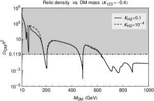
Figure 2: Figures displaying the dependence of $\Omega_{\textrm{DM}}h^{2}$ on $M_{\textrm{DM}}$, for $\kappa_{\textrm{123}}=-0.4$ (the figure on the left) and $\kappa_{\textrm{123}}=-0.1$ (the figure on the right). Each figure shows two cases corresponding to $\kappa_{H\textrm{2}}=10^{-1},10^{-4}$. The dot-dashed line is the Planck $\Omega_{\textrm{DM}}h^{2}$. The gray region means the DM candidate would be excluded, and the white one means that the DM candidate can still make some part of the DM content of the Universe.

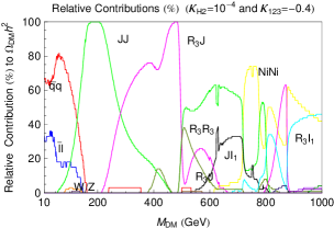
Figure 3: (Color online) Figures displaying the relative contributions (%) of the main annihilation channels to the DM relic abundance. The cases with $\kappa_{H\textrm{2}}=10^{-1},\,10^{-4}$ and $\kappa_{\textrm{123}}=-0.1,\,-0.4$ are shown.

In order to better comprehend the annihilation processes and their contributions contained in the curves in Fig. 2, we plot Fig. 3 which shows the relative contributions to $\Omega_{\textrm{DM}}h^{2}$ of the main DM annihilation channels. Let’s consider some relevant regions. For $M_{\textrm{DM}}$ less than $80$ GeV we have in general two resonances. The first one is due to the interchange of the $Z_{1}$ gauge boson in the $s-$channel. It is located at $M_{\textrm{DM}}=M_{Z_{1}}/2\approx 45.6$ GeV and remains there even when $\kappa_{H2}$ is set to $10^{-4}$. It is so because it depends on the $N_{\textrm{DM}}-N_{\textrm{DM}}-Z_{1}$ coupling via neutral currents. Since this coupling arises from the covariant derivatives, it is independent on the $\kappa_{H2}$ value. In contrast, the second resonance, which arises by the $s-$channel interchange of the Higgs boson (located in $m_{\text{Higgs}}/2\approx 62.5$ GeV), disappears when $\kappa_{H2}=10^{-4}$. This is understood realizing that $N_{\textrm{DM}}$ couples to the Higgs boson via the term $\frac{1}{2}\frac{\sqrt{2}M_{\textrm{DM}}}{V_{\phi}}\overline{(n_{R3})^{c}}n_{R3}\phi_{2}$ and since Higgs component in $\phi_{2}$ depends on $\kappa_{H2}$, it is clear that the smaller $\kappa_{H2}$ the smaller $N_{\textrm{DM}}-N_{\textrm{DM}}-$Higgs coupling. In this region of masses we also notice that $N_{\textrm{DM}}$ annihilation processes into quark-antiquark pair (in special into $b\bar{b}$ quarks for $\kappa_{H2}=10^{-1}$) are the dominant for both figures. These occur via Higgs mediation. Annihilation processes into neutrinos via the $Z_{1}$ interchange are also important ($\sim 25\%$). This is also true for both values of $\kappa_{H2}$ and for both $\kappa_{\textrm{123}}=-0.4$ and $-0.1$.

As $M_{\textrm{DM}}$ increases from $80\,\textrm{GeV}$ to $120$ GeV, and as long as $\kappa_{\textrm{123}}=-0.4$ and $\kappa_{H2}=10^{-1}$, the annihilation into gauge bosons ($W^{\pm}/Z_{1}$) are dominant (in particular into $W^{+}W^{-}$) with some considerable ($\sim 20\%$) contribution of annihilation into quark-antiquark pair. In contrast, for $\kappa_{\textrm{123}}=-0.4$ and $\kappa_{H2}=10^{-4}$, the $N_{\textrm{DM}}$ annihilation processes into quark-antiquark pairs continue being the most important. Moreover, $N_{\textrm{DM}}$ annihilation processes into $JJ$ start to be considerable ($\sim 15\%$). Similar conclusions are true for the case of $\kappa_{123}=-0.1$ and $\kappa_{H2}=10^{-1}$. However, for this case, annihilations into gauge bosons ($W^{\pm}/Z_{1}$) have a little lower contribution when compared to the case $\kappa_{123}=-0.4$. For the case of $\kappa_{123}=-0.1$ and $\kappa_{H2}=10^{-4}$, the annihilations into antiquarks-quarks are the most contributing.

In the region $120\,\textrm{GeV}\leq M_{\textrm{DM}}\leq 180\,\textrm{GeV}$ and with $\kappa_{\textrm{123}}=-0.4$ and $\kappa_{H2}=10^{-1}$, roughly speaking, three $N_{\textrm{DM}}$ annihilation processes are similarly predominant. These are annihilations into $W^{+}W^{-}/Z_{1}Z_{1}$, $R_{1}R_{1}$ and $JJ$. Recall that $R_{1}$ is the Higgs-like scalar. For this region of mass and with $\kappa_{\textrm{123}}=-0.1$ and $\kappa_{H2}=10^{-1}$ analogous conclusions can be reached. This is not the case for $\kappa_{H2}=10^{-4}$ (with $\kappa_{\textrm{123}}=-0.4$) in the same $M_{\textrm{DM}}$ region, in which case, $N_{\textrm{DM}}$ annihilations into $JJ$ are almost completely dominant with an additional contribution ($\sim 12\%$) from the annihilations into quark-antiquark pairs. For $\kappa_{\textrm{123}}=-0.1$ and $\kappa_{H2}=10^{-4}$, however, we find that annihilation into quark-antiquark pairs are still dominant.

As $M_{\textrm{DM}}$ is around $m_{R_{3}}/2\approx 205$ GeV, we see a resonance, in Fig. 2 on the left, due $R_{3}$ $s-$channel interchange for both $\kappa_{H2}$ values. Here, predominant annihilation process is $N_{\textrm{DM}}N_{\textrm{DM}}\rightarrow JJ$ with more than $50\%$ of contribution. It is also important to note that for a $M_{\textrm{DM}}$ in this region we have the $\Omega_{\textrm{DM}}h^{2}$ value reported by Planck. This resonance does not occur in the $\kappa_{123}=-0.1$ cases because $m_{R_{3}}\approx 1114.61$ GeV. However, in these cases, we have one resonance at $m_{I_{2}}/2\approx 242.6$ GeV, with $N_{\textrm{DM}}N_{\textrm{DM}}\rightarrow R_{1}J$ as dominant process for $\kappa_{H2}=10^{-1}$, and with $N_{\textrm{DM}}N_{\textrm{DM}}\rightarrow\bar{q}q$ as dominant process, for $\kappa_{H2}=10^{-4}$.

In the region $220\,\textrm{GeV}\leq M_{\textrm{DM}}\leq 500\,\textrm{GeV}$ and with $\kappa_{\textrm{123}}=-0.4$ and $\kappa_{H2}=10^{-1}$, we can say that two annihilations, $N_{\textrm{DM}}N_{\textrm{DM}}\rightarrow JJ$ and $N_{\textrm{DM}}N_{\textrm{DM}}\rightarrow R_{3}J$, strongly control $\Omega_{\textrm{DM}}h^{2}$. Except when $M_{\textrm{DM }}\approx m_{I_{2}}/2\approx 485.1\,\textrm{GeV}$ where $N_{\textrm{DM}}N_{\textrm{DM}}\rightarrow R_{3}J$ annihilation completely governs $\Omega_{\textrm{DM}}h^{2}$. As $500\,\textrm{GeV}<M_{\textrm{DM}}\leq 700\,\textrm{GeV}$, annihilations into $JJ$, $R_{1}I_{1}$, $R_{3}R_{3}$, $R_{3}J$ and $JI_{1}$ are predominant and their contributions depend on the proximity to the three different resonances. Finally, when $700\,\textrm{GeV}<M_{\textrm{DM}}\leq 1000\,\textrm{GeV}$, annihilations into $JJ$, $R_{3}I_{1}$, $R_{3}J$, $N_{1}N_{1}$ and $N_{2}N_{2}$ are the most contributing processes to determine $\Omega_{\textrm{DM}}h^{2}$. Similar behavior is found for the case $\kappa_{\textrm{123}}=-0.4$ and $\kappa_{H2}=10^{-4}$. It is so because in these regions of masses the annihilation processes mostly depend on the trilinear vertices between scalars.

As $\kappa_{\textrm{123}}=-0.1$ and $\kappa_{H2}=10^{-1}$, the scalar spectrum changes and thus the location of the resonances change as well. As it was commented, the resonance at $m_{R_{3}}/2\approx 205\,\textrm{GeV}$ does not exist anymore. Instead, we have a resonance at $m_{I_{2}}/2\approx 242.6$ GeV. In the region $220\,\textrm{GeV}\leq M_{\textrm{DM}}\leq 470\,\textrm{GeV}$, the most important difference, in contrast with the case $\kappa_{\textrm{123}}=-0.4$, is that we do not have regions with $\Omega_{\textrm{DM}}h^{2}\leq 0.119$ (a little tiny region can be seen in the $m_{I_{2}}/2\approx 242.6\,\textrm{GeV}$). Another difference is that annihilation into $W^{+}W^{-}/Z_{1}Z_{1}$ remains to be important in this region ($\sim 15\%-35\%$). In addition, annihilation into $R_{1}I_{1}$ contributes $>35\%$ in most of this mass region. Other annihilations, such as $R_{1}J$, $I_{1}I_{1}$, $JJ$ and $R_{1}R_{1}$, also contribute but are subdominant. For $470\,\textrm{GeV}\leq M_{\textrm{DM}}\leq 700\,\textrm{GeV}$, $\Omega_{\textrm{DM}}h^{2}$ is completely determined by annihilation into $I_{1}I_{1}$, $I_{1}J$, $JJ$. As $700\,\textrm{GeV}\leq M_{\textrm{DM}}\leq 1000\,\textrm{GeV}$, annihilation processes into $N_{1}N_{1}$ and $N_{2}N_{2}$ share importance with $I_{1}I_{1}$, $R_{3}I_{1}$, $R_{4}I_{1}$ and $R_{5}I_{1}$ to determine $\Omega_{\textrm{DM}}h^{2}$. For $M_{\textrm{DM}}>470\,\textrm{GeV}$, we have $\Omega_{\textrm{DM}}h^{2}\leq 0.119$.

Finally, when $\kappa_{\textrm{123}}=-0.1$ and $\kappa_{H2}=10^{-4}$, we have some relevant differences. What is clearest is that for $M_{\textrm{DM}}<470\,\textrm{GeV}$ we just have the $Z_{1}$ resonance, which depends only on the VEVs and the $g$’s. This is because of the smallness of $\kappa_{\textrm{123}}$ and $\kappa_{H2}$ (specially $\kappa_{H2}=10^{-4}$), which makes the couplings with these $CP-$odd scalar mediators be tiny. Some features are worth mentioning, though. Up to $M_{\textrm{DM}}\simeq 350\,\textrm{GeV}$, annihilation into quarks are predominant. After that, until $M_{\textrm{DM}}\simeq 700\,\textrm{GeV}$, the final products $I_{1}I_{1}$, $I_{1}J$, $JJ$ (summing $\sim 35-100\%$) enter as the major contributors to the relic density and the quarks enter as subdominant processes fading out at $M_{\textrm{DM}}\simeq 450\,\textrm{GeV}$. Next, up to $M_{\textrm{DM}}\simeq 900\,\textrm{GeV}$, the main annihilation products are $N_{1}N_{1}$ and $N_{2}N_{2}$ ($\sim 30-40\%$ each), with $R_{3}I_{1}$ taking place at the end of this interval. Finally, for $850\,\textrm{GeV}\leq M_{\textrm{DM}}\leq 1000\,\textrm{GeV}$, the main contributions come from $R_{3}I_{1}$, $R_{4}I_{1}$ and $R_{5}I_{1}$, summing more than $70\%$ of the DM annihilation energy.

Now, in order to grasp the behavior of the relic density when one varies $\kappa_{\textrm{123}}$, we show a two-dimensional figure, Fig. 4, which was obtained with ${\tt MicrOMEGAs}$, from a $10^{5}$ points iteration. We see from it that as one varies $\kappa_{\textrm{123}}$, the regions for correct relic density (cyan points), change place, getting to the minimal value of $M_{\textrm{DM}}\sim 200\textrm{ GeV}$ for $\kappa_{\textrm{123}}=-0.4$; and also for some points which increases in $\kappa_{123}$ as $M_{\textrm{DM}}$ decreases, having at $\kappa_{\textrm{123}}\sim-0.05$ its last point. We can also notice green regions (together with cyan lines) that extend from left to right as $M_{\textrm{DM}}$ increases, and the reason behind it are the resonances of $I_{2}$, $I_{3}$ (decrease as $\kappa_{\textrm{123}}$ increases) and $R_{3}$ (increases). Therefore, one can conclude that the correct relic density, before $M_{\textrm{DM}}\sim 500-600\,\textrm{GeV}$, may only be reached through resonances of the lightest singlet particles of our spectrum.

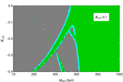
Figure 4: (Color online) 2-D figure displaying the behavior of $\Omega_{\textrm{DM}}h^{2}$ as one continuously varies both $\kappa_{\textrm{123}}$ in the range $[-0.4,\,0]$, with $\kappa_{H\textrm{2}}=0.1$, and $M_{\textrm{DM}}$ in the range $[10,\,1000]\,$ GeV. The cyan points represent correct relic density $\Omega_{\textrm{DM}}h^{2}$, within experimental errors; the green ones indicate $\Omega_{\textrm{DM}}h^{2}$ below the Planck result; and the gray ones mean $\Omega_{\textrm{DM}}h^{2}$ above Planck constraint and thus ruled out.

V.2 Direct Detection

Figure 5: Figures displaying the curves representing the SI cross section per nucleon, $\sigma_{\textrm{SI-nucleon}}$, asa function of $M_{\textrm{DM}}$, for the $N_{\textrm{DM}}$ elastic scattering off nucleon. Cases for $\kappa_{\textrm{123}}=-0.4;\,-0.1$ and $\kappa_{H\textrm{2}}=10^{-1},10^{-2}$ are shown. In these figures, we also display the SI upper limits coming from LUX (dashed), XENON100 (dot-dashed) and SuperCDMS (dotted). All $\sigma_{\textrm{SI-nucleon}}$ curves in the gray region are ruled out by the LUX upper limit.

Other important constraints on DM candidates come from the current experiments (XENON100_2012, ; SuperCDMS_2014, ; LUX_2014, ) which aim to directly detect WIMP dark matter by measuring the kinetic energy transferred to a nucleus after it scatters off a DM particle. All of these experiments have imposed limits on the WIMP scattering cross section off the nuclei. In general, the WIMP-nucleus interactions can be either spin-independent (SI) or spin-dependent (SD). Currently, the most constraining limits come from the Large Underground Xenon (LUX) experiment (LUX_2014, ) which has set bounds on the SI WIMP-nucleon elastic scattering with a minimum upper limit on the cross section of $7.6\times 10^{-10}$ pb at a WIMP mass of $33$ GeV$/c^{2}$.

We have verified that, for $N_{\textrm{DM}}$ considered here, the dominant interactions are SI. Thus, we calculate (using the ${\tt MicrOMEGAs}$ package) the SI elastic scattering cross section per nucleon, $\sigma_{\textrm{SI-nucleon}}$, and the results are shown in Fig. 5. Actually, we scale the $\sigma_{\textrm{SI-nucleon}}$ cross sections with the calculated relic density relative to that measured by the Planck in order to properly compare the predicted cross sections with those given by direct detection experiments, which present their results assuming the observed density. The experimental limits on SI cross sections are also shown in Fig. 5. We have not shown results for SD cross sections because we found that those are, in general, several orders under the SI current limits, see Refs. (COUPP_SD_DD, ; SIMPLE-II_SD_DD, ) which state a minimum upper bound of $\sim 5\times 10^{-3}\,\textrm{pb}$ at a WIMP mass of $24\,\textrm{GeV}/c^{2}$.

From Fig. 5, it can be seen that the smaller $\kappa_{H2}$, the smaller $\sigma_{\textrm{SI-nucleon}}$. As $\kappa_{H2}=10^{-2}$ the $\sigma_{\textrm{SI-nucleon}}$ is below the LUX upper bound for all values of $M_{\textrm{DM}}$. For $\kappa_{H2}=10^{-1}$ and $M_{\textrm{DM}}\lesssim 500$ GeV, $\sigma_{\textrm{SI-nucleon}}$ is below the LUX limit only around the resonances. In contrast, for $M_{\textrm{DM}}\gtrsim 500$ GeV, the LUX limits are satisfied for all cases shown in Fig. 5. This implies that $\sigma_{\textrm{SI-nucleon}}$ mainly depends on $\kappa_{H2}$. This fact is easily understood by realizing that, in our case, the relevant interactions for direct detection are mostly mediated via Higgs in the t-channel . Thus, these interactions depend on the mixings between the Higgs scalar ($R_{1}$) and rest of $R_{i}$ scalars. These mixings strongly depend on the $\kappa_{H2}$ value, as it was already discussed. In addition, we can see from Fig. 5 that although $\sigma_{\textrm{SI-nucleon}}$ (actually $\sigma_{\textrm{SI-nucleon}}\times\Omega_{\textrm{DM}}h^{2}/0.1193$ ) does not depend directly on other scalars, there is clearly indirect dependence on them because these scalars affect the annihilation cross section and thus the relic abundance.

Finally, from Figs. 2 and 5 we can conclude that, provided $\kappa_{H2}\lesssim 10^{-2}$, the constraints coming from the $\Omega_{\textrm{DM}}h^{2}$ determine if a set of parameters leads to a viable dark matter candidate or not.

VI conclusions

In this paper, we have discussed a scenario where neutrino masses and dark matter are possible. In particular, the model presented here is a gauge extension of the SM based on $\text{SU}(2)_{L}\otimes\text{U}(1)_{Y^{\prime}}\otimes\text{U}(1)_{\mathcal{B-L}}$ symmetry group. Besides the SM fields, we have added one doublet scalar ($\Phi$), four singlet scalars ($\phi_{i}$), and three right-handed neutrinos ($n_{Ri}$). These three last fields have different quantum numbers under the gauge groups and more importantly, they couple to different scalars. This allows a rich texture in the neutrino mass matrices. In addition, because of the exclusion of one term from the Lagrangian, we have that a $\mathbb{Z}_{2}$ symmetry acting only in $n_{R3}$ appears. This opens the possibility that $n_{R3}$ be a DM candidate.

The model contains a very rich scalar sector, and in special, we find that it contains a Majoron, $J$, which has its origin in a global accidental symmetry, U$\left(1\right)_{J}$. We show that this symmetry is exact and it acts on the total Lagrangian. Despite the fact that global symmetries can be broken by gravity quantum effects, we have not considered that possibility in this paper. Thus, the Majoron remains massless and in principle, it poses some issues to the safety of the model. Therefore, we study the consequences of the presence of $J$ in the physical spectrum. Specifically, we consider four major challenges: (i) energy loss in stars by the process $\gamma+e^{-}\rightarrow e^{-}+J$ (geJ_stars1, ; geJ_stars2, ); (ii) relativistic degrees of freedom in the Universe, parametrized by $N_{\textrm{eff}}$; (iii) $Z$ invisible decay width; and (iv) Higgs invisible decay width. Setting $V_{\phi}=1$ TeV and $V_{H}\simeq V_{\textrm{SM}}=246$ GeV, the first of these constraints leads to $\epsilon=V_{\Phi}/V_{\phi}\lesssim 3.8\times 10^{-4}$ (where we have set all VEVs of scalar singlets equal). The second constraint really does not lead to any restriction on the parameters of the model since the $J$ contribution to the density of radiation in the Universe is in agreement with the Planck limits (PLANCK_2013, ) for different decoupling temperatures. The issue of the $Z$ invisible width is also overcome by imposing some constraints on the scalar potential parameters as shown in Secs. III and V. In addition, the Higgs invisible decay width is maintained at $\textrm{Br}_{\textrm{Higgs}}^{\textrm{Inv}}\apprle 10-15\%$ (Ellis_2013, ; Giardino2014, ; Atlascollaboration, ; CMScollaboration, ) provided that $\kappa_{H2}<0.2$. Finally, since $\epsilon\ll 1$, we have shown an overview of the scalar spectra by expanding the scalar squared-mass matrices in powers of $\epsilon$ and doing other simplifying considerations.

Since $\epsilon$ has to be very small, we can use the well-known see-saw approximation to analytically solve the ${\cal D}_{ij}$ and $\mathcal{M}_{ij}$ parameters. These are found by imposing some experimental constraints coming from the neutrino physics. In special, the mixing angles and the differences of the squared neutrino masses. We manage to solve the ${\cal D}_{ij}$ and $\mathcal{M}_{ij}$ parameters by making the ansatz that $M_{\nu}$ matrix is diagonalized by the tri-bimaximal-Cabbibo matrix. It is important to note that the existence of the $\mathbb{Z}_{2}$ symmetry makes easier to solve the equations because there appears a massless light neutrino. In general, we find all ${\cal D}_{ij}$ parameters depend on the dimensional constant $K=\frac{V_{\phi}^{2}\epsilon^{2}}{2M_{N}}$. It is true for both normal and inverted mass hierarchies. One more interesting result is reached when we take into consideration the LFV processes such as $\textrm{Br}\left(\mu\rightarrow e+\gamma\right)$ and $\textrm{Br}\left(\tau\rightarrow\mu+\gamma\right)$. The current bounds (Olive:2014PDG, ) on these processes constrain $\epsilon$. For the normal case, one obtains $\epsilon\apprge 1.97\times 10^{-6}$, and for the inverted case $\epsilon\gtrsim 1.58\times 10^{-6}$. We also have checked that $\sum_{i=1}^{3}m_{\nu_{i}}<0.23\,\textrm{eV}$, coming from Planck (PLANCK_2013, ), and the effective Majorana mass bound $m_{ee}<0.27-0.65\,\textrm{GeV}$ (mee_future, ; mee_CUORE_2015, ), coming from double beta decay experiments, were satisfied.

After the scalar and neutrino sectors of the model were studied and many of the parameters were set, we consider the $n_{R3}$ (more precisely $N_{\textrm{DM}}$) as a DM candidate. We study the bounds coming from the relic density abundance $\Omega_{\textrm{DM}}h^{2}$ (PLANCK_2013, ) and the direct detection experiments (LUX_2014, ; XENON100_2012, ; SuperCDMS_2014, ). Basically, we have worked with three free parameters, $\kappa_{H2}$ , $\kappa_{123}$, and the DM mass, $M_{\textrm{DM}}$. These parameters have been chosen because they play a very important role in determining both the $N_{\textrm{DM}}$ annihilation cross section and the $N_{\textrm{DM}}$ elastic scattering off the nucleon. Roughly speaking, we find that for $M_{\textrm{DM}}\lesssim 500$ GeV, the $\Omega_{\textrm{DM}}h^{2}\leq 0.1193$ is achieved around the resonance regions. For $M_{\textrm{DM}}>500$ GeV there are several regions with $\Omega_{\textrm{DM}}h^{2}\leq 0.1193$ aside from resonances regions. This is understood by realizing that the couplings of $N_{\textrm{DM}}$ to scalars (including the Higgs) are proportional to $\frac{\sqrt{2}M_{\textrm{DM}}}{2V_{\phi}}$, and that for $M_{\textrm{DM}}<200$ GeV the main annihilation channels are, in general, mediated by the Higgs. It is also observed, that making $\kappa_{123}$ bigger, we obtain more regions with $\Omega_{\textrm{DM}}h^{2}\leq 0.1193$ for smaller $M_{\text{DM}}$. This is because $\kappa_{123}$ strongly controls the trilinear couplings between scalars and thus, the annihilation cross section is larger when $\kappa_{123}$ is larger. We have found that the relative contributions to the DM annihilation in this model have an intricate pattern. It strongly depends on the scalar masses. However, some general conclusions can be drawn. For $M_{\textrm{DM }}\leq 200$ GeV the annihilation into $\bar{q}q$, $W/Z$, $\bar{l}l$ are dominant. For $200<M_{\textrm{DM}}<700$ GeV annihilations into scalars are the most important. Finally, for $700\,\text{GeV}<M_{\textrm{DM}}$ annihilations into $N_{i}N_{i}$ play a important role.

For DM direct detection, the parameter $\kappa_{H2}$ is the most relevant since it is the only one which effectively couples $N_{\textrm{DM}}$ to the quarks in our model. Since nuclei are made of quarks (and gluons), this interaction is of supreme importance to the elastic scattering of $N_{\textrm{DM}}$ off nuclei. We found out that if we choose $\kappa_{H2}=10^{-2}$, our entire curves are below LUX data, the most stringent upper bounds on SI DD, however if one chooses a riskier value such as $\kappa_{H2}=0.1$, it can still be lower than LUX, however only above $M_{\textrm{DM}}\sim 500-600\,\textrm{GeV}$ or at the resonances below that $M_{\textrm{DM}}$.

A final remark concerning to the $Z_{2}$ gauge boson is in order. In the region of parameters that we have studied, the $Z_{2}$ boson does not affect the DM properties. It is because $Z_{2}$ is heavy since its mass has to satisfy $M_{Z_{2}}/g_{B-L}\apprge 6\,\textrm{TeV}$ (MZ2_1, ; MZ2_2, ). In addition, its mixing angle in the neutral current is limited to be $\tan\beta\apprle 10^{-3}$ (beta_1, ; beta_2, ; beta_3, ).

Appendix A THE MINIMIZATION

The general minimization conditions coming from $\partial V_{{\cal{B}-{\cal{L}}}}/\partial R_{i}=0$, where $V_{{\cal{B}-{\cal{L}}}}$ is the scalar potential in Eq. (2) and $R_{i}=\{H_{R}^{0},\,\Phi_{R}^{0},\,\phi_{1R},\,\phi_{2R},\,\phi_{3R},\,\phi_{XR}\}$ are the neutral real components of the scalar fields, can be written as:

$$0 = V_{H}\left(2\lambda_{H}V_{H}^{2}+\kappa_{H\Phi}V_{\Phi}^{2}+\kappa_{H1}V_{\phi_{1}}^{2}+\kappa_{H2}V_{\phi_{2}}^{2}+\kappa_{H3}V_{\phi_{3}}^{2}+\kappa_{HX}V_{\phi_{X}}^{2}-2\mu_{H}^{2}\right)$$ (19)

$$-\sqrt{2}\kappa_{H\Phi X}V_{\Phi}V_{\phi_{X}};$$

$$0 = V_{\Phi}\left(\kappa_{H\Phi}V_{H}^{2}+2\lambda_{\Phi}V_{\Phi}^{2}+\kappa_{\Phi 1}V_{\phi_{1}}^{2}+\kappa_{\Phi 2}V_{\phi_{2}}^{2}+\kappa_{\Phi 3}V_{\phi_{3}}^{2}+\kappa_{\Phi X}V_{\phi_{X}}^{2}-2\mu_{\Phi}^{2}\right)$$ (20)

$$-\sqrt{2}\kappa_{H\Phi X}V_{H}V_{\phi_{X}};$$

$$0 = V_{\phi_{1}}\left(\kappa_{H1}V_{H}^{2}+\kappa_{\Phi 1}V_{\Phi}^{2}+2\lambda_{1}V_{\phi_{1}}^{2}+\kappa_{12}V_{\phi_{2}}^{2}+\kappa_{13}V_{\phi_{3}}^{2}+\kappa_{1X}V_{\phi_{X}}^{2}-2\mu_{1}^{2}\right)$$ (21)

$$+V_{\phi_{2}}V_{\phi_{3}}\left(\kappa_{123}V_{\phi_{3}}+\kappa_{123X}V_{\phi_{X}}\right);$$

$$0 = V_{\phi_{2}}\left(\kappa_{H2}V_{H}^{2}+\kappa_{\Phi 2}V_{\Phi}^{2}+\kappa_{12}V_{\phi_{1}}^{2}+2\lambda_{2}V_{\phi_{2}}^{2}+\kappa_{23}V_{\phi_{3}}^{2}+\kappa_{2X}V_{\phi_{X}}^{2}-2\mu_{2}^{2}\right)$$ (22)

$$+V_{\phi_{1}}V_{\phi_{3}}\left(\kappa_{123}V_{\phi_{3}}+\kappa_{123X}V_{\phi_{X}}\right);$$

$$0 = V_{\phi_{3}}\left(\kappa_{H3}V_{H}^{2}+\kappa_{\Phi 3}V_{\Phi}^{2}+\kappa_{13}V_{\phi_{1}}^{2}+\kappa_{23}V_{\phi_{2}}^{2}+2\lambda_{3}V_{\phi_{3}}^{2}+\kappa_{3X}V_{\phi_{X}}^{2}+3\kappa^{\prime}_{3X}V_{\phi_{3}}V_{\phi_{X}}\right.$$ (23)

$$\left.-2\mu_{3}^{2}\right)+V_{\phi_{1}}V_{\phi_{2}}\left(2\kappa_{123}V_{\phi_{3}}+\kappa_{123X}V_{\phi_{X}}\right);$$

$$0 = V_{\phi_{X}}\left(\text{$\kappa_{HX}$}V_{H}^{2}+\text{$\kappa_{\Phi X}$}V_{\Phi}^{2}+\kappa_{1X}V_{\phi_{1}}^{2}+\text{$\kappa_{2X}$}V_{\phi_{2}}^{2}+\text{$\kappa_{3X}$}V_{\phi_{3}}^{2}+2\text{$\lambda_{X}$}V_{\phi_{X}}^{2}-2\mu_{X}^{2}\right)$$ (24)

$$-\sqrt{2}\text{$\kappa_{H\Phi X}$}V_{\Phi}V_{H}+V_{\phi_{3}}\left(\kappa_{123X}V_{\phi_{1}}V_{\phi_{2}}+\kappa^{\prime}_{3X}V_{\phi_{3}}^{2}\right).$$

References

- [1] Y. Fukuda et al. (Super-Kamiokande collaboration). Evidence for Oscillation of Atmospheric Neutrinos. Phys. Rev. Lett., 81:1562–1567, 1998. arXiv:hep-ex/9807003.
- [2] Q. R. et al. (SNO collaboration) Ahmad. Direct Evidence for Neutrino Flavor Transformation from Neutral-Current Interactions in the Sudbury Neutrino Observatory. Phys. Rev. Lett., 89:011301, 2002. arXiv:nucl-ex/0204008.
- [3] T. Araki et al. (KamLAND collaboration). Measurement of Neutrino Oscillation with KamLAND: Evidence of Spectral Distortion. Phys. Rev. Lett., 94:081801, 2005. arXiv:hep-ex/0406035.
- [4] P. Adamson et al. (MINOS collaboration). Measurement of Neutrino Oscillations with the MINOS Detectors in the NuMI Beam. Phys. Rev. Lett., 101:131802, 2008. arXiv:0806.2237 [hep-ex].
- [5] P. A. R. Ade et al. (PLANCK collaboration). Planck 2013 results. XVI. Cosmological parameters. 2013. arXiv:1303.5076 [astro-ph.CO].
- [6] S. F. King and C. Luhn. Neutrino mass and mixing with discrete symmetry. Reports on Progress in Physics, 76(5):056201, 2013. arXiv:1301.1340 [hep-ph].
- [7] O. J. P. Éboli, J. Gonzalez-Fraile, and M.C. Gonzalez-Garcia. Neutrino masses at LHC: minimal lepton flavour violation in Type-III see-saw. Journal of High Energy Physics, 2011(12), 2011. arXiv:1108.0661 [hep-ph].
- [8] H. Baer, A. D. Box, and H. Summy. Mainly axion cold dark matter in the minimal supergravity model. Journal of High Energy Physics, 2009(08):080, 2009. arXiv:0906.2595 [hep-ph].
- [9] K. J. Bae, H. Baer, and E. J. Chun. Mixed axion/neutralino dark matter in the SUSY DFSZ axion model. Journal of Cosmology and Astroparticle Physics, 2013(12):028, 2013. arXiv:1309.5365 [hep-ph].
- [10] E. Ma. Verifiable radiative seesaw mechanism of neutrino mass and dark matter. Phys. Rev. D, 73:077301, 2006. arXiv:hep-ph/0601225.
- [11] K. M. Zurek. Multicomponent dark matter. Phys. Rev. D, 79:115002, 2009. arXiv:0811.4429 [hep-ph].
- [12] D. S. Akerib et al. (LUX collaboration). First Results from the LUX Dark Matter Experiment at the Sanford Underground Research Facility. Phys. Rev. Lett., 112:091303, 2014. arXiv:1310.8214 [astro-ph.CO].
- [13] E. Aprile et al. (XENON collaboration). Dark Matter Results from 225 Live Days of XENON100 Data. Phys. Rev. Lett., 109:181301, 2012. arXiv:1207.5988 [astro-ph.CO].
- [14] R. Agnese et al. (SuperCDMS collaboration). Search for Low-Mass Weakly Interacting Massive Particles Using Voltage-Assisted Calorimetric Ionization Detection in the SuperCDMS Experiment. Phys. Rev. Lett., 112:041302, 2014. arXiv:1309.3259 [physics.ins-det].
- [15] A. Geringer-Sameth and S. M. Koushiappas. Exclusion of Canonical Weakly Interacting Massive Particles by Joint Analysis of Milky Way Dwarf Galaxies with Data from the Fermi Gamma-Ray Space Telescope. Phys. Rev. Lett., 107:241303, 2011. arXiv:1108.2914 [astro-ph.CO].
- [16] M. Ackermann et al. (Fermi-LAT Collaboration). Constraining Dark Matter Models from a Combined Analysis of Milky Way Satellites with the Fermi Large Area Telescope. Phys. Rev. Lett., 107:241302, 2011. arXiv:1108.3546 [astro-ph.HE].
- [17] M. Ackermann et al. (Fermi-LAT Collaboration). Dark matter constraints from observations of 25 Milky Way satellite galaxies with the Fermi Large Area Telescope. Phys. Rev. D, 89:042001, 2014. arXiv:1310.0828 [astro-ph.HE].
- [18] M. Ackermann et al. (Fermi-LAT Collaboration). Searching for Dark Matter Annihilation from Milky Way Dwarf Spheroidal Galaxies with Six Years of Fermi-LAT Data. 2015. arXiv:1503.02641 [astro-ph.HE].
- [19] S. Galli, F. Iocco, G. Bertone, and A. Melchiorri. Updated CMB constraints on dark matter annihilation cross sections. Phys. Rev. D, 84:027302, 2011. arXiv:1106.1528 [astro-ph.CO].
- [20] J. C. Montero and V. Pleitez. Gauging U(1) symmetries and the number of right-handed neutrinos. Phys.Lett., B675:64–68, 2009.
- [21] J. C. Montero and B. L. Sánchez-Vega. Neutrino masses and the scalar sector of a B-L extension of the standard model. Phys.Rev., D84:053006, 2011.
- [22] B. L. Sánchez-Vega, J. C. Montero, and E. R. Schmitz. Complex scalar dark matter in a - model. Phys. Rev. D, 90:055022, 2014.
- [23] M. Aoki, S. Kanemura, and O. Seto. Model of TeV scale physics for neutrino mass, dark matter, and baryon asymmetry and its phenomenology. Phys. Rev. D, 80:033007, 2009. arXiv:0904.3829 [hep-ph].
- [24] M. Lindner, D. Schmidt, and T. Schwetz. Dark Matter and neutrino masses from global symmetry breaking. Physics Letters B, 705(4):324–330, 2011. arXiv:1105.4626 [hep-ph].
- [25] Howard Georgi and S. L. Glashow. Unity of All Elementary-Particle Forces. Phys. Rev. Lett., 32:438–441, 1974.
- [26] Paul Langacker. The physics of heavy gauge bosons. Rev. Mod. Phys., 81:1199–1228, 2009. arXiv:0801.1345 [hep-ph].
- [27] M. Cvetič, D. A. Demir, J. R. Espinosa, L. Everett, and P. Langacker. Electroweak breaking and the problem in supergravity models with an additional U(1). Phys. Rev. D, 56:2861–2885, 1997. arXiv:hep-ph/9703317.
- [28] Paul Langacker. Grand unified theories and proton decay. Physics Reports, 72(4):185 – 385, 1981.
- [29] R. N. Mohapatra. Unification and Supersymmetry. The frontiers of quark-lepton physics. 1986. Springer.
- [30] D. A. Dicus, E. W. Kolb, V. L. Teplitz, and R. V. Wagoner. Astrophysical bounds on the masses of axions and Higgs particles. Phys. Rev. D, 18:1829–1834, 1978.
- [31] G. G. Raffelt (Particle Data Group). Axions and other very light bosons: part II (astrophysical constraints). 2006.
- [32] J. Ellis and T. You. Updated global analysis of Higgs couplings. Journal of High Energy Physics, 2013(6), 2013. arXiv:1303.3879 [hep-ph].
- [33] Pier Paolo Giardino, Kristjan Kannike, Isabella Masina, Martti Raidal, and Alessandro Strumia. The universal Higgs fit. Journal of High Energy Physics, 2014(5), 2014.
- [34] G. Aad et al. (Atlas collaboration). Search for Invisible Decays of a Higgs Boson Produced in Association with a Boson in ATLAS. Phys. Rev. Lett., 112:201802, 2014.
- [35] S. Chatrchyan and et al. (CMS collaboration). Search for invisible decays of Higgs bosons in the vector boson fusion and associated ZH production modes. The European Physical Journal C, 74(8), 2014.
- [36] K. A. Olive et al. (Particle Data Group). Review of Particle Physics. Chinese Phys. C, 38(9):090001, 2014.
- [37] J. J. Gómez-Cadenas et al. Sense and sensitivity of double beta decay experiments. Journal of Cosmology and Astroparticle Physics, 2011(06):007, 2011. arXiv:1010.5112 [hep-ex].
- [38] K. Alfonso et al. (CUORE experiment). Search for Neutrinoless Double-Beta Decay of 130Te with CUORE-0. 2015. arXiv:1504.02454[nucl-ex].
- [39] S. L. Glashow and S. Weinberg. Natural conservation laws for neutral currents. Phys. Rev. D, 15:1958–1965, 1977.
- [40] T. P. Cheng and M. Sher. Mass-matrix ansatz and flavor nonconservation in models with multiple Higgs doublets. Phys. Rev. D, 35:3484–3491, 1987.
- [41] G. Gilbert. Wormhole-induced proton decay. Nuclear Physics B, 328(1):159 – 170, 1989.
- [42] R. Holman, S. D. H. Hsu, T. W. Kephart, E. W. Kolb, R. Watkins, and L. M. Widrow. Solutions to the strong-CP problem in a world with gravity. Physics Letters B, 282(1-2):132 – 136, 1992.
- [43] M. Kamionkowski and J. March-Russell. Planck-scale physics and the Peccei-Quinn mechanism . Physics Letters B, 282(1-2):137 – 141, 1992.
- [44] E. Kh. Akhmedov et al. Planck scale effects on the majoron. Physics Letters B, 299(1-2):90–93, 1993. arXiv:hep-ph/9209285.
- [45] J. C. Montero and B. L. Sánchez-Vega. Natural Peccei-Quinn symmetry in the 3-3-1 model with a minimal scalar sector. Phys. Rev. D, 84:055019, 2011.
- [46] M. C. Gonzalez-Garcia and Y. Nir. Implications of a Precise Measurement of the Width on the Spontaneous Breaking of Global Symmetries. Phys.Lett., B232:383, 1989.
- [47] Steven Weinberg. Goldstone Bosons as Fractional Cosmic Neutrinos. Phys. Rev. Lett., 110:241301, 2013.
- [48] E. Ma and M. Raidal. Neutrino Mass, Muon Anomalous Magnetic Moment, and Lepton Flavor Nonconservation. Phys. Rev. Lett., 87:011802, 2001. arXiv:hep-ph/0102255.
- [49] P. Gondolo and G. Gelmini. Cosmic abundances of stable particles: Improved analysis. Nuclear Physics B, 360(1):145 – 179, 1991.
- [50] K. Griest and D. Seckel. Three exceptions in the calculation of relic abundances. Phys. Rev. D, 43:3191–3203, 1991.
- [51] A. Alloul et al. FeynRules 2.0 - A complete toolbox for tree-level phenomenology. Computer Physics Communications, 185(8):2250–2300, 2014. arXiv:1310.1921 [hep-ph].
- [52] A. Belyaev, N. D. Christensen, and A. Pukhov. CalcHEP 3.4 for collider physics within and beyond the Standard Model. Computer Physics Communications, 184(7):1729–1769, 2013. arXiv:1207.6082 [hep-ph].
- [53] G. Bélanger et al. micrOMEGAs 4.1: Two dark matter candidates. Computer Physics Communications, 192(0):322–329, 2015. arXiv:1407.6129 [hep-ph].
- [54] J. Erler et al. Improved constraints on bosons from electroweak precision data. Journal of High Energy Physics, 2009(08):017, 2009. arXiv:0906.2435 [hep-ph].
- [55] F. del Aguila, J. de Blas, and M. Pérez-Victoria. Electroweak limits on general new vector bosons. Journal of High Energy Physics, 2010(9), 2010. arXiv:1005.3998 [hep-ph].
- [56] R. Diener, S. Godfrey, and I. Turan. Constraining extra neutral gauge bosons with atomic parity violation measurements. Phys. Rev. D, 86:115017, 2012. arXiv:1111.4566 [hep-ph].
- [57] T. Appelquist, B. A. Dobrescu, and A. R. Hopper. Nonexotic neutral gauge bosons. Phys. Rev. D, 68:035012, 2003. arXiv:hep-ph/0212073.
- [58] M. Carena et al. gauge bosons at the Fermilab Tevatron. Phys. Rev. D, 70:093009, 2004. arXiv:hep-ph/0408098.
- [59] E. Behnke et al. (COUPP collaboration). First dark matter search results from a 4-kg bubble chamber operated in a deep underground site. Phys. Rev. D, 86:052001, 2012. arXiv:1204.3094.
- [60] M. Felizardo et al. (SIMPLE collaboration). Final Analysis and Results of the Phase II SIMPLE Dark Matter Search. Phys. Rev. Lett., 108:201302, 2012. arXiv:1106.3014.