Quantum-classical transition and quantum activation of ratchet currents in the parameter space

Abstract

The quantum ratchet current is studied in the parameter space of the dissipative kicked rotor model coupled to a zero temperature quantum environment. We show that vacuum fluctuations blur the generic isoperiodic stable structures found in the classical case. Such structures tend to survive when a measure of statistical dependence between the quantum and classical currents are displayed in the parameter space. In addition, we show that quantum fluctuations can be used to overcome transport barriers in the phase space. Related quantum ratchet current activation regions are spotted in the parameter space. Results are discussed based on quantum, semiclassical and classical calculations. While the semiclassical dynamics involves vacuum fluctuations, the classical map is driven by thermal noise.

I Introduction

A general description of unbiased transport of particles in nature, which is named ratchet effect, is a challenging issue with implications in distinct areas, such as in molecular motors in biology F.Jülicher et al. (1997), nanosystems like graphene C.Drexler et al. (2013), control of cancer metastasis G.Mahmud et al. (2009), micro and nanofluids T.Kulrattanarak et al. (2011), particles in silicon membrane pores S.Matthias and F.Müller (2003), cold atoms G.G.Carlo et al. (2005), solids and drops transport using the Leidenfrost effect G.Lagubeau et al. (2011); Linke et al. (2006), quantum systems Reimann et al. (1997); Schanz et al. (2001); D.Bercioux et al. (2008); Jonckheere et al. (2003), among many others. Certainly the most relevant and common goal in describing these ratchet systems is to unveil how to control and attain an efficient transport by choosing the appropriate physical parameter combination, like temperature, dissipation, external forces etc. It is known Schanz et al. (2001) that in classical conservative systems the parameters must be chosen so that the underlying dynamics presents a mixture of regular and chaotic motion. In dissipative inertial systems the Classical Ratchet Current (CRC) is more efficient when parameters are chosen inside the Isoperiodic Stable Structures (ISSs), which appear in the parameter space of ratchet models A.Celestino et al. (2011, 2013). Such ISSs are generic Lyapunov stable islands with dynamics globally structurally stable and come along in many dynamical systems J.A.C.Gallas (1993); Zou et al. (2006); Lorenz (2008); R.Stoop et al. (2010); Gallas (2010). When stochastic effects are included, e. g. thermal fluctuations, these ISSs start to be destroyed and become blurred, even though they remain resistant to reasonable noise intensities Manchein et al. (2013). This means that in realistic systems the CRC is more efficient when parameters are chosen inside the ISSs. In Manchein et al. (2013) it was also shown that in certain multistability scenarios the current may actually be thermally activated.

The natural question now is whether the same general statements can be made regarding the relation between the system’s parameters (or the ISSs) and the Quantum Ratchet Current (QRC). With the ongoing technological developments engineering smaller and smaller devices this question becomes crucial for the observation of directed transport in quantum systems. It has been shown G.G.Carlo (2012) that for specific points in the parameter space the QRC  apparently has the same main properties of the CRC  inside the ISSs when considered with a certain finite temperature (see also G.G.Carlo et al. (2005)). In this context one expects the quantum version of the ISSs to become blurred and gradually disappear as the full quantum limit is reached. In principle though, the simple addition of thermal effects in the classical dynamics is certainly not enough to reproduce the quantum dynamics.

In the present work we calculate the QRC  using a dissipative zero temperature master equation. Therefore, fluctuations are of quantum origin while no thermal noise is considered in the description. In the semiclassical limit, the master equation can be recast as a semiclassical map, allowing us to study in details the quantum-classical transition. The semiclassical results are compared to the classical map for the ratchet system, derived through direct integration of the Langevin equation over a kicking period. The classical map involves correlated thermal fluctuations. We show how and to which extent the quantum-classical transition affects the optimal currents inside the ISSs. Even though vacuum fluctuations destroy the well defined shape of the ISSs when the current is plotted, the borders of the structures tend to survive when the quantum and classical currents are statistically compared Székely et al. (2007). In addition, the quantum fluctuations can assist current activation and we spot the activated regions in the parameter space.

The paper is structured in the following way. In Sec. II we present the quantum, semiclassical and classical models used to investigate the ratchet current. In Sec. III the results for the quantum ratchet current, its activation, and the distance correlations are shown in the parameter space and discussed. Section IV presents the summary of our findings and motivates related experiments.

II Models

II.1 The Quantum Problem

The quantum problem can be described using the kicked Hamiltonian in dimensionless units

$$\hat{\cal H}=\frac{\hat{p}^{2}}{2}+K\left[\cos{(\hat{x})}+\tfrac{1}{2}\cos{(2\,\hat{x}+\tfrac{\pi}{2})}\right]\sum_{m=0}^{+\infty}\delta(t-m\tau),$$ (1)

where ($\hat{x},\hat{p}$) are position and momentum operators, $m=1,2,\ldots,N$ represents the discrete times when the “kicks” occur, $\tau$ is the kicking period, and $K$ is the parameter which controls the intensity of the kick. Dissipation is introduced between the kicks by coupling the ratchet system to a zero temperature environment. In usual Born-Markov approximation a master equation for the reduced dynamics is obtained T.Dittrich and R.Graham (1990). Here we determine the corresponding density operator as an ensemble mean over pure states obtained from the corresponding quantum state diffusion Gisin and Percival (1992) Ito-stochastic Schrödinger equation

$$|d\psi\rangle = -{i}\hat{\cal H}|\psi\rangle dt+\sum_{\mu}\left(L_{\mu}-\langle L_{\mu}\rangle\right)|\psi\rangle d\xi_{\mu}$$

$$-\frac{1}{2}\sum_{\mu}\left(L_{\mu}^{\dagger}L_{\mu}-2\langle L_{\mu}^{\dagger}\rangle L_{\mu}+|\langle L_{\mu}\rangle|^{2}\right)|\psi\rangle dt,$$

where $\langle.\rangle$ stands for the expectation value. The Lindblad operators are given by $\hat{L}_{1}=g\sum_{n}\sqrt{n+1}\left|n\right>\left<n+1\right|,$ and $\hat{L}_{2}=g\sum_{n}\sqrt{n+1}\left|-n\right>\left<-n-1\right|,$ with $g$ being the coupling constant and $n=0,1,\ldots$. The $|n\rangle$ states are the eigenstates of the momentum operator $\hat{p}|n\rangle=2\pi\,n|n\rangle$. The Lindblad operators induce a damping $-\lambda\langle\hat{p}\rangle$, with rate $\lambda=g^{2}$. The semiclassical limit of (1) and (LABEL:SE) is obtained by taking $\tau\to 0$ and $\lambda\to\infty$, such that the dissipation parameter $\gamma=e^{-\lambda\tau}$ remains constant. It turns out that $\hbar_{eff}=\tau$ plays the role of the effective Planck constant G.G.Carlo et al. (2005). The QRC  is obtained from $\bf C_{Q}=||\langle\hat{p}\rangle||$, where $||.||$ is a double average, over quantum realizations and time. As initial condition (IC) we use a coherent wave packet localized inside a minimum of the ratchet potential, i. e. $\left<\hat{x}_{0}\right>=\pi/2$ with $\langle\hat{n}_{0}\rangle=0.0$.

II.2 The Semiclassical Problem

We can better understand the quantum-classical relation regarding the directed transport by studying the QRC  as we approach the classical limit $\hbar_{eff}\to 0$. It is not reasonable, however, to perform a full quantum calculation for this purpose because it is numerically too demanding since more and more states and a huge number of time steps must be taken into account in this limit. To overcome this difficulty we use the semiclassical map proposed years ago T.Dittrich and R.Graham (1990) for the standard map. In our ratchet case the semiclassical map at zero temperature takes the form

$$\tilde{p}_{m+1} = \gamma\,\tilde{p}_{m}+\gamma\,K\left\{\sin{(\tilde{q}_{m}+\tilde{\psi}_{m+1})}\right.$$ (4)

$$+ \left.\frac{1}{2}\,\sin{\left[2(\tilde{q}_{m}+\tilde{\psi}_{m+1})+\frac{\pi}{2}\right]}\right\}+\tilde{\eta}_{m+1},$$ (6)

$$\tilde{q}_{m+1} = \tilde{q}_{m}+\frac{(1-\gamma)\tau}{\gamma|ln\gamma|}\tilde{p}_{m+1}+\tilde{\psi}_{m+1},$$

where ($\tilde{x}_{m},\tilde{p}_{m}$) are scalars being the position and momentum at discrete times $m=1,2,\ldots,N$, and $K$ is the kicking parameter. The map (6) and the noise sources ($\tilde{\psi}_{m+1},\tilde{\eta}_{m+1}$) arise from conveniently writing the propagator of the Wigner function as a quasi-stochastic map (for more details see T.Dittrich and R.Graham (1990)). The noise terms are uncorrelated in time and satisfy $\langle\tilde{\eta}_{m+1}\rangle=\langle\tilde{\psi}_{m+1}\rangle=0$, and

$$\langle\tilde{\eta}_{m+1}^{2}\rangle=\gamma\,(1-\gamma)\,\hbar_{eff}|\tilde{p}_{m}|/(2\pi),$$ (7)

(8)

$$\langle\tilde{\psi}_{m+1}^{2}\rangle=\frac{4\,(1-\gamma)\,\hbar_{eff}}{\gamma|\tilde{p}_{m}|}+\frac{\gamma\,\hbar_{eff}|\tilde{p}_{m}|}{2\pi(1-\gamma)|ln\gamma|^{2}}\left[|ln\gamma|^{2}\right.$$ (9)

(10)

$$\qquad\qquad\left.-2(1-\gamma)|ln\gamma|+(1-\gamma)^{2}(1-\frac{2}{\gamma})|ln\gamma|\right.$$ (11)

(12)

$$\qquad\qquad\left.+\frac{2}{\gamma}(1-\gamma)^{3}+\frac{(1-\gamma)^{4}}{\gamma^{2}})\right],$$ (13)

(14)

$$\langle\tilde{\eta}_{m+1}\tilde{\psi}_{m+1}\rangle=\frac{\gamma\,|\tilde{p}_{m}|\hbar_{eff}}{2\pi}\left[1-\frac{(1-\gamma)}{|ln\gamma|}-\frac{(1-\gamma)^{2}}{\gamma|ln\gamma|}\right].$$

Higher order cumulants were neglected (higher orders in $\hbar_{eff}$) so that the map (6) can be interpreted as a classical map with Gaussian noise terms of quantum mechanical origin. This map is valid as long $\hbar_{eff}\ll 1$. The current obtained from (6) is referred to as SRC (Semiclassical Ratchet Current). ICs with $\langle\langle x_{0}\rangle\rangle=\langle\langle p_{0}\rangle\rangle=0$ were taken inside the unit cell $(-2\pi,2\pi)$.

II.3 The Classical Problem

The connection between the dynamics of a quantum system at zero temperature and its finite temperature classical limit in the parameter space is not obvious at first sight. Although one could argue that the first-order (in $\hbar$) quantum correction to a classical system is equivalent to a white noise term Strunz and Percival (1998), the fluctuation-dissipation relation can differ, and it is also not clear whether a certain region of the parameter space would require higher order corrections for a reliable description of the system’s dynamics. We access this connection by means of a direct comparison between the calculated current in parameter space for the quantum system and its classical finite temperature limit. This limit is obtained via integration of the kicked Langevin equation

$$\dot{p} = -\lambda p+K\left[\sin{(x)}+\frac{1}{2}\sin(2\,x+\frac{\pi}{2})\right]\sum_{n=0}^{\infty}\delta(t-n\tau_{c})$$ (16)

$$+\sigma\xi(t),$$

$$\dot{x} = p,$$

where $\tau_{c}$ is the classical kicking time, $\sigma=\sqrt{2\lambda k_{B}T}$, and $\xi(t)$ is the white noise satisfying $\langle\xi(t)\rangle=0$ and $\langle\xi(t)\xi(s)\rangle=\delta(t-s)$. The integration is performed between two kicks of the potential including the kick in the beginning, but not the one at the end. More precisely, the integration is performed between $t_{0}=m-\epsilon$ and $t=m+1-\epsilon$, with positive $\epsilon\rightarrow 0$. Defining $\gamma=\exp(-\lambda\tau_{c})$, the integration produces the following map

$$p_{m+1} = \gamma p_{m}+\gamma K\left[\sin{(x_{m})}+\frac{1}{2}\sin(2\,x_{m}+\frac{\pi}{2})\right]+\alpha_{m},$$ (17)

$$x_{m+1} = x_{m}+\frac{(1-\gamma)\tau_{c}}{\gamma|\ln{\gamma}|}p_{m+1}+\beta_{m},$$ (19)

with the two stochastic terms ($\alpha_{m},\beta_{m}$) featuring the properties $\langle\alpha_{m}\rangle=\langle\beta_{m}\rangle=0,$ and

$$\langle\alpha_{m}^{2}\rangle = \frac{\,T_{eff}}{\tau_{c}}(1-\gamma^{2}),$$ (20)

$$\langle\beta_{m}^{2}\rangle = \frac{T_{eff}}{\gamma^{2}|\ln{\gamma}|^{2}}\left(2\gamma^{2}|\ln{\gamma}|+3\gamma^{2}-4\gamma+1\right),$$ (21)

$$\langle\alpha_{m}\beta_{m}\rangle = -\frac{T_{eff}}{\tau_{c}\gamma|\ln{\gamma}|}(1-\gamma)^{2},$$

with $T_{eff}=k_{B}T\tau_{c}^{2}$. In the map, the variables $x_{m}$ and $p_{m}$ represent respectively the position and the kinetic momentum of the particle when it is kicked by the $m$-th time ($m=1,2,...,N$). Notice that the correlated thermal noise in the map (LABEL:mapC), derived from the kicked Langevin equation with white noise, differs from the uncorrelated noise used in previous works G.G.Carlo (2012); Manchein et al. (2013). As in the semiclassical case, ICs with $\langle\langle x_{0}\rangle\rangle=\langle\langle p_{0}\rangle\rangle=0$ were taken inside the unit cell $(-2\pi,2\pi)$.

III Results

III.1 Ratchet current

Now we can discuss results by comparing the currents of the three problems above. Figure 1 shows the ratchet currents (see colors) (a) $\bf C_{Q}$ (quantum), (b) $\bf C_{S}$ (semiclassical) and (c)-(d) $\bf C_{C}$ (classical) in the parameter space ($K^{\prime},\gamma$) with $K^{\prime}=(1-\gamma)\tau\,K/|\ln{\gamma}|$ being the rescaled kick parameter. In order to compare $\bf C_{S}$  and $\bf C_{C}$  with the $\bf C_{Q}$,  we used ${\bf C_{S}}=(1-\gamma)\tau/(\gamma|\ln\gamma|)||\tilde{p}||$ and ${\bf C_{C}}=(1-\gamma)\tau/(\gamma|\ln\gamma|)||p||$, where the double average is over ICs and time. We checked that the $\bf C_{Q}$  converges, for the whole considered parameter space, after $10^{3}$ kicks and some tens of stochastic realizations. For the semiclassical and classical simulations we used $10^{4}$ iterations and $10^{3}$ ICs with zero average in position and momentum. It is worth to mention that for the parameter $\gamma$, shown in Fig. 1(a), the damping $\lambda$ is approximately inside the interval [$2.0,9.7$], which represents strong dissipation. Thus the quantum dynamics is incoherent after the very short classical times $m_{r}\approx 1/(1-\gamma)$ T.Dittrich and R.Graham (1990) and coherence effects are not expected to be relevant for the results shown in the parameter space from Fig. 1(a).

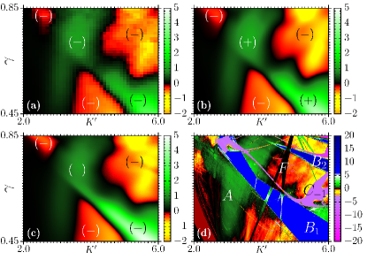
Figure 1: (Color online) The parameter spaces showing the (a) $\bf C_{Q}$, (b) $\bf C_{S}$, for $\hbar_{eff}=0.082$, and (c) $\bf C_{C}$  for $T_{eff}=0.082$. Red (green) to yellow (white) colors are related to increasing negative (positive) currents [marked with ($-$) and ($+$) for the printed grayscale]. Note the black boundaries delimiting positive and negative currents. In (d) we have the $\bf C_{C}$  for $T_{eff}=0$ with black colors related to close to zero currents; green to blue colors (light to dark gray) are related to increasing positive currents while red, yellow to purple (white to light gray) colors related to increasing negative currents. Letters denote the chaotic background $A$ and the ISSs $B_{1},B_{2},C_{-1}$ and $F$.

Agreement between $\bf C_{Q}$ [Fig. 1(a)] and $\bf C_{S}$ [Fig. 1(b)] is astonishing, meaning that the semiclassical map (6) nicely reproduces the quantum results in the quantum-classical transition for this range of parameters. Note that the $\bf C_{C}$  in Fig. 1(c), obtained using one fixed $T_{eff}$ in the classical map (LABEL:mapC), also shows a qualitative agreement with the $\bf C_{Q}$.

To understand the physical origin of the distinct currents in Figs. 1(a)-(c) we analyze the $\bf C_{C}$  at zero temperature $T_{eff}=0$. This is shown in Fig. 1(d). Two main regions with distinct behaviors can be observed: first, the “cloudy” background, identified as $A$ in Fig. 1(d) showing a mixture of zero, small negative and positive currents, where the dynamics is chaotic A.Celestino et al. (2013). Second, the four ISSs, $B_{1},B_{2}$, $C_{-1}$ and $F$. Besides $F$, which has zero current, the ISSs are responsible for the optimal $\bf C_{C}$ and can be recognized by their sharp borders (for a detailed explanation see A.Celestino et al. (2011, 2013)). We note that at the crossing regions of $B_{1}$ and $F$, positive currents are observed as a consequence of multistable attractors. The portion of the parameter space shown in Fig. 1 can be regarded as representative of the highly dissipative ratchet regime of this system, presenting the main properties found in the larger parameter space, and is thus suitable for the purpose of the present work. Comparing Figs. 1(a)-(c) to Fig. 1(d), we can identify that the positive and negative $\bf C_{Q}$, $\bf C_{S}$ and $\bf C_{C}$ ($T_{eff}>0$) roughly follow the overall chaotic currents from the region $A$, but are enhanced inside the ISS $B_{1}$ from the classical case with $T_{eff}=0$. This shows that vacuum fluctuations tend to blur the classical ISSs, as suggested recently G.G.Carlo (2012).

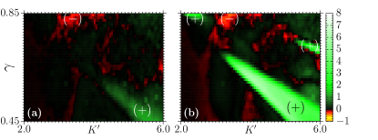
Figure 2: (Color online) Plotted is (a) $|\mbox{$\bf C_{S}$}|-|\mbox{$\bf C_{Q}$}|$ and (b) $|\mbox{$\bf C_{C}$}|-|\mbox{$\bf C_{Q}$}|$ from the data of Fig. 1 [Symbols ($-$)/($+$) to identify the negative/positve currents in printed grayscale].

One can recover many of the $\bf C_{Q}$’s features in parameter space using classical calculations. This was also observed in G.G.Carlo (2012), for specific points in the parameter space, in a system in contact with a distinct thermal bath with uncorrelated noise. However, while a purely classical map with thermal fluctuations (and single $T_{eff}$ value) leads to a $\bf C_{C}$  that can qualitatively mimic $\bf C_{Q}$  in parameter space, it is usually quantitatively very far off. Much better agreement, both qualitatively and quantitatively, is reached using a semiclassical map. This is shown in Fig. 2. We stress that quantum results are very well represented by the semiclassical map without any free parameter. By contrast, the simulation in terms of the classical approach (LABEL:mapC), involves $T_{eff}$ as an additional free parameter that needs to be adjusted for every point in the parameter space to achieve an overall agreement with the $\bf C_{Q}$. Thus, it becomes clear that a single $T_{eff}$ is not able to reproduce the $\bf C_{Q}$  for the whole parameter space.

III.2 Correlation between SRC  and CRC

A result for the quantum-classical transition regarding ratchet currents is found by analyzing the correlation between the $\bf C_{S}$ (at $\hbar_{eff}\neq 0$) and the $\bf C_{C}$ (at $T_{eff}=0$). It is a measure of statistical dependence, called distance correlation Székely et al. (2007), between both currents, which is zero if and only if the currents are statistically independent. Thus, the purpose of the present analysis is to search to which extent the quantum current is statistically similar to the classical current. For this we use the distance correlation, which is obtained from the expression Székely et al. (2007) ${\cal D}{(\tilde{p},p)}=d{(\tilde{p},p)}/\sqrt{\Delta({\tilde{p}})\Delta({p})}$, where

$$d{(\tilde{p},p)}=\frac{1}{N}\sqrt{\sum_{j,k=1}^{N}\,{S}_{j,k}{C}_{j,k}}$$ (22)

is the distance covariance, and

$$\Delta(\tilde{p})=\frac{1}{N}\sqrt{\sum_{j,k}^{N}\,({S}_{j,k})^{2}},\quad\Delta(p)=\frac{1}{N}\sqrt{\sum_{j,k}^{N}\,({C}_{j,k})^{2}},$$ (23)

are the distance variances. Here $\tilde{p}$ refers to the time sequence ${\tilde{p}}_{1},\tilde{p}_{2},\tilde{p}_{3},\ldots,\tilde{p}_{m}$ obtained from the map (6), leading to the $\bf C_{S}$. $p$ refers to the time sequence $p_{1},p_{2},p_{3},\ldots,p_{m}$ obtained from the map (LABEL:mapC), leading to the $\bf C_{C}$. $S$ and $C$ are matrices defined through ${S}_{j,k}=s_{j,k}-\overline{s}_{j.}-\overline{s}_{.k}+\overline{s}_{..}$ and ${C}_{j,k}=c_{j,k}-\overline{c}_{j.}-\overline{c}_{.k}+\overline{c}_{..}$, respectively. Here $s_{j,k}=|\overline{\tilde{p}}_{j}-\overline{\tilde{p}}_{k}|$ is the Euclidean norm of the distance between the momenta (averaged over ICs) at times $j$ and $k$. Thus, $\overline{\tilde{p}}_{j}$ is an average over ICs at times $j$. The same is valid for $c_{j,k}=|\overline{p}_{j}-\overline{p}_{k}|$. In addition, $\overline{s}_{j.}$ is the $j$-th row mean, $\overline{s}_{.k}$ the $k$-th column mean, and $s_{..}$ is the mean value between $\overline{s}_{j.}$ and $\overline{s}_{.k}$ (the same notation applies to $c$). Thus, each element of the matrices $S$ and $C$ contains information about: distances in time of the currents (already averaged over ICs) and also time averages of these distances over the time series $\tilde{p}$ and $p$. The distance correlation ${\cal D}{(\tilde{p},p)}$, on the other hand, analyses the statistical independence of both matrices. It is not a direct quantity to be measured in one simulation (or experiment), but compares the currents obtained by two simulations performed in distinct semiclassical regimes.

In Figs. 3 (a) and (b) the quantity ${\cal D}{(\tilde{p},p)}$ is displayed (colors) in the same parameter space from Fig. 1. White, yellow, red to blue (white, light to dark-gray) colors are related to increasing values of the distance correlation. For each point in the parameter space we used $N=4.5\times 10^{3}$ points of the time sequence of $\tilde{p}_{m}$ and $p_{m}$, averaged over $5\times 10^{4}$ ICs.

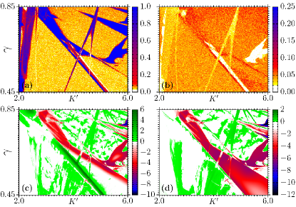
Figure 3: (Color online) Plotted is ${\cal D}{(\tilde{p},p)}$ for (a) $\hbar_{eff}=0.0001$ and (b) $\hbar_{eff}=0.082$, and the activation/suppression $\delta(\hbar_{eff})$ for (c) $\hbar_{eff}=0.01$ and (d) $\hbar_{eff}=0.082$.

At small $\hbar_{eff}=0.0001$ we observe in the parameter space for ${\cal D}{(\tilde{p},p)}$ that the structures $B_{1},B_{2},C_{-1},F$ can be clearly recognized (they have sharp borders). For parameters inside the ISSs the quantum-classical dynamics is strongly correlated, while outside the ISSs the correlation goes to zero. Inside the ISS $B_{1}$ we observe that correlations also go to zero, but its border is still well defined. For $\hbar_{eff}=0.082$ the result is inverted, as inside most part of the ISSs the correlation is zero and outside it remains almost the same as from Fig. 3 (a). In this case the ISS $B_{2}$ disappeared, the $C_{-1}$ and $F$ yet exist with sharp borders, and some remaining borders of $B_{1}$ are visible. These results demonstrate that the sharp borders of the ISSs tend to survive in the parameter space (for reasonable $\hbar_{eff}$) when ${\cal D}{(\tilde{p},p)}$ is plotted, while the ISSs are already blurred and unrecognizable when the ratchet current is plotted [compare Fig. 3(b) to Figs. 1(a) and (b)]. In other words, the way the ISSs disappear in both cases is fundamentally distinct. It is obvious that using huge values for $\hbar_{eff}$ the correlation in the whole parameter space will go to zero.

III.3 Quantum activation of the ratchet current

Another interesting related phenomenon is that the quantum fluctuations not only lower the $\bf C_{S}$, but also activate them. In order to show this we calculate $\delta(\hbar_{eff})=|\mbox{$\bf C_{S}$}(\hbar_{eff})|-|\mbox{$\bf C_{C}$}(T_{eff}=0)|$ and plot a map of the current activation/suppression in the parameter space. For $\delta>0$ activation of the $\bf C_{S}$  occurs while for $\delta<0$ the $\bf C_{S}$  decreases due to vacuum fluctuations. Results are shown in Fig. 3(c) and (d) for the same parameter space from Fig. 1. We use green to dark-green (gray to dark-gray) colors for increasing activations of the $\bf C_{S}$ and white, red, blue to black (white, dark-gray to black) for increasing suppressions of $\bf C_{S}$. Surprisingly there are many regions in the parameter space where activations occur. The physical origin of the activations depend on the specific dynamics at a given parameter combination. Along the diagonal dark-green line (below the ISS $B_{1}$) where large activations ($\Delta\sim 6$) occur in Fig. 3(c), we conclude from classical results A.Celestino et al. (2011) that the activation is due to a crisis bifurcation. Additional numerical results revealed that the activation close to $K=2.5$ and $\gamma=0.85$ is related to a symmetry breaking of the multistable attractors.

IV Conclusions

Concluding, the quantum ratchet current was analyzed in the parameter space of the asymmetrically kicked rotor. We have shown that isoperiodic stable structures with sharp borders play an essential role in the quantum-classical transition. Quantum currents were obtained numerically exact by solving the Markov stochastic Schrödinger Eq. (LABEL:SE)($\bf C_{Q}$), and in a semiclassical approach from the semiclassical map (6)($\bf C_{S}$). For the classical currents ($\bf C_{C}$) we used the map (LABEL:mapC) which was derived via direct integration of the kicked Langevin equation with a white noise. The quantum-classical transition was studied by means of a comparison between the $\bf C_{S}$  and $\bf C_{C}$. We show how and to which extent the classical generic isoperiodic stable structures A.Celestino et al. (2011, 2013); Manchein et al. (2013) are destroyed by quantum fluctuations. Even though these structures become blurred and start to disappear in the quantum world, their sharp borders tend to persist when the correlation between quantum and classical currents is investigated. For this aim we have used the distance correlation measure Székely et al. (2007). Remarkably we have found a statistical dependence of the quantum and classical currents when parameters are chosen at the borders of the isoperiodic stable structures. Moreover, very often this dependence extends to the interior of the isoperiodic structures. In addition, we calculated the quantum activation/suppression of the current in the parameter space. Surprisingly many regions were found where quantum fluctuations enhance the $\bf C_{C}$. Even though the distance correlation and the current activation are not directly observed for one simulation or experiment, they can be obtained by comparing two simulations in distinct semiclassical regimes and allow us to understand better the quantum-classical transition of ratchet currents.

It is generally accepted that dissipative quantum dynamics inducing decoherence will blur any quantumness and eventually will lead to a dynamics that may well be described in classical terms. In this paper we show, however, that for the ratchet current in a zero-temperature environment, this quantum-classical transition is far from trivial and depends crucially on the chosen parameters. We prove that a replacement of quantum fluctuations by classical thermal fluctuations is overly simplistic and cannot be used for the whole parameter space uniformly. It is clear that a single quantity like the $\bf C_{Q}$  can be matched by a $\bf C_{C}$  if one allows an additional free parameter (here temperature) to vary. Crucially, however, different points in parameter space require very different temperatures for this fit procedure (see Fig. 2), and in this sense a quantum-classical correspondence, where quantum fluctuations are replaced by thermal fluctuations, cannot exist. In addition, there is no one scaling which gives the quantum-classical correspondence in the whole parameter space. One of the reasons for this behavior can be traced back to the complicated dynamics in the case of mixed phase space structure. In our context we can write $\bf C_{S}=\sum_{i}\alpha_{i}\bf C_{S}^{(i)}$, where the sum is over the attractors, $\bf C_{S}^{(i)}$ is the ratchet current from attractor $i$ weighted by the area of the corresponding basin of attraction, and $\alpha_{i}=\mu_{i}\tau_{i}$ is the statistical weight of each attractor, where $\tau_{i}$ is the mean lifetime on attractor $i$ and $\mu_{i}=lim_{n\to\infty}\langle m_{i}\rangle/n$ where $m_{i}$ is the number of times a given trajectory visited the attractor $i$ during the time $n$. Quantum fluctuations allow the trajectory to jump between attractors and $\alpha_{i}$ is the quantity which depends, in a nontrivial way, on $h_{eff}$ and may also depend on the size/shape of the basin of attraction. The degree of quantum-classical correspondence is therefore strongly dependent on the local dynamics, and general statements about the scaling of $\alpha_{i}$ are difficult. However, our results indicate a qualitatively different correspondence for parameters inside and outside the ISS regions. Indeed, we have shown that the way the ratchet current responds to the quantum fluctuations depends sensitively on whether the parameters are chosen within the ISSs’ limits. It indicates that the classical-quantum transition is much more abrupt inside the ISSs, at least regarding the ratchet current.

Our results are an important step towards the goal to experimentally observe quantum isoperiodic structures in the context of ratchet effects with cold atoms C.Mennerat-Robilliard et al. (1999); Shrestha et al. (2011). Moreover, we strongly believe that quantum activations deserve further analysis, both theoretically and experimentally. In general, the analysis of the complex quantum-classical transition in the parameter space (including the isoperiodic structures), is not restricted to ratchet currents. Other observable of a quantum system, whose classical counterpart presents regular and chaotic dynamics, could be used. We mention for example the motion of atoms in an optical lattice Cavalcante et al. (2005); Thommen et al. (2011) and the electronic wave-packet dynamics in Rydberg atoms subjected to a strong static magnetic field Alber and Zoller (1991); Beims and Alber (1993, 1996).

V Acknowledgments

Our international cooperation is supported by PROBRAL - DAAD/CAPES and M.W.B. and C.M. thank CNPq for financial support and M.W.B. thanks MPIPKS in the framework of the Advanced Study Group on Optical Rare Events.

References

- F.Jülicher et al. (1997) F.Jülicher, A.Ajdari, and J.Prost, Rev.Mod.Phys. 1997, 1269 (1997).
- C.Drexler et al. (2013) C.Drexler, S. A. Tarasenko, P. Olbrich, J. Karch, M. Hirmer, F. Müller, M. Gmitra, J. Fabian, R. Yakimova, S. Lara-Avila, et al., Nature Nanotechnology 8, 104 (2013).
- G.Mahmud et al. (2009) G.Mahmud, C.J.Campbell, K.J.M.Bishop, Y.A.Komarova, O.Chaga, S.Soh, S.Huda, K.Kandere-Grzybowska, B.A.Grzybowski, and A.Bartosz, Nature Physics 5, 606 (2009).
- T.Kulrattanarak et al. (2011) T.Kulrattanarak, R. der Sman, C.G.P.H.Schroen, and R.M.Boom, Microfluidics and Nanofluidics 10, 843 (2011).
- S.Matthias and F.Müller (2003) S.Matthias and F.Müller, Nature 424, 53 (2003).
- G.G.Carlo et al. (2005) G.G.Carlo, G.Benenti, G.Casati, and D.L.Shepelyansky, Phys.Rev.Lett. 94, 164101 (2005).
- G.Lagubeau et al. (2011) G.Lagubeau, M. L. Merrer, C. Clanet, and D. Quere, Nature Physics 7, 395 (2011).
- Linke et al. (2006) H. Linke, B. J. Alemnán, L. D. Melling, M. J. Taormina, M. J. Francis, C. C. Dow-Hygelund, V. Narayanan, R. P. Taylor, and A. Stout, Phys. Rev. Lett. 96, 154502 (2006).
- Reimann et al. (1997) P. Reimann, M. Grifoni, and P. Hanggi, Phys. Rev. Lett. 79, 10 (1997).
- Schanz et al. (2001) H. Schanz, M.-F. Otto, R. Ketzmerick, and T. Dittrich, Phys. Rev. Lett. 87, 070601 (2001).
- D.Bercioux et al. (2008) D.Bercioux, M. Grifoni, and K.Richter, Phys.Rev.Lett. 100, 230601 (2008).
- Jonckheere et al. (2003) T. Jonckheere, M. R. Isherwood, and T. S. Monteiro, Phys. Rev. Lett. 91, 253003 (2003).
- A.Celestino et al. (2011) A.Celestino, C. Manchein, H.A.Albuquerque, and M.W.Beims, Phys.Rev.Lett. 106, 234101 (2011).
- A.Celestino et al. (2013) A.Celestino, C. Manchein, H.A.Albuquerque, and M.W.Beims, Commun. Nonlinear Sci. Numer. Simul. 19, 139 (2013).
- J.A.C.Gallas (1993) J.A.C.Gallas, Phys.Rev.Lett. 70, 2714 (1993).
- Zou et al. (2006) Y. Zou, M. Thiel, M. C. Romano, J. Kurths, and Q. Bi, Int. J. Bif. Chaos 16, 3567 (2006).
- Lorenz (2008) E. N. Lorenz, Physica D 237, 1689 (2008).
- R.Stoop et al. (2010) R.Stoop, P.Benner, and Y.Uwate, Phys.Rev.Lett. 105, 074102 (2010).
- Gallas (2010) J. A. C. Gallas, Int. J. Bif. Chaos 20, 197 (2010).
- Manchein et al. (2013) C. Manchein, A. Celestino, and M.W.Beims, Phys.Rev.Lett. 110, 114102 (2013).
- G.G.Carlo (2012) G.G.Carlo, Phys.Rev.Lett. 108, 210605 (2012).
- Székely et al. (2007) G. Székely, M. Rizzo, and N. Barikov, The Annals of Statistics 35, 2769 (2007).
- T.Dittrich and R.Graham (1990) T.Dittrich and R.Graham, Annals of Physics 200, 363 (1990).
- Gisin and Percival (1992) N. Gisin and I. C. Percival, J. Phys. A: Math. Gen. 25, 5677 (1992).
- Strunz and Percival (1998) W. T. Strunz and I. C. Percival, Journal of Physics A: Mathematical and General 31, 1801 (1998).
- C.Mennerat-Robilliard et al. (1999) C.Mennerat-Robilliard, D.Lucas, S.Guibal, J.Tabosa, C.Jurczak, J.-Y.Courtois, and G.Grynberg, Phys.Rev.Lett. 82, 851 (1999).
- Shrestha et al. (2011) R. K. Shrestha, J. Ni, W. K. Lam, S. Wimberger, and G. S. Summy, Phys. Rev. A 86, 043617 (2011).
- Cavalcante et al. (2005) H. L. S. Cavalcante, C. R. Carvalho, and J. C. Garreau, Phys. Rev. A 72, 033814 (2005).
- Thommen et al. (2011) Q. Thommen, J. C. Garreau, and V. Zehnlé, Phys. Rev. A 84, 043403 (2011).
- Alber and Zoller (1991) G. Alber and P. Zoller, Phys. Rep. 199, 231 (1991).
- Beims and Alber (1993) M. W. Beims and G. Alber, Phys. Rev. A 48, 3123 (1993).
- Beims and Alber (1996) M. W. Beims and G. Alber, J. Phys. B 29, 4139 (1996).