Abstract

We provide explicit partial differential equations – in finite cases – and functional differential equations – in field-theoretic cases – which determine observables or beables in the senses of Kuchař and of Dirac. These cover a wide range of relational mechanics models as well as Electromagnetism, Yang–Mills Theory and General Relativity. We give an underlying reason why pure-configuration Kuchař observables are already well-known: various types of shape, E-fields, B-fields, loops and 3-geometries. The partial differential equations or functional differential equations for pure-momentum observables are also posed, as are those for observables which have a mixture of configuration and momentum functional dependence.

PACS 04.20.Cv, 04.20.Fy

^∗ Dr.E.Anderson.Maths.Physics *at* protonmail.com

1 Introduction

This article concerns specific physically and geometrically significant examples of constrained theories [2, 3, 4]. Let $Q^{\mbox{{\scriptsize A}}}$ denote the theory’s configurations, the possible values of which form its configuration space $\mathfrak{q}$. The corresponding conjugate momenta are denoted by $P_{\mbox{{\scriptsize A}}}$. The joint space of the $Q^{\mbox{{\scriptsize A}}}$ and $P_{\mbox{{\scriptsize A}}}$, as equipped with the classical bracket |[ , ]| constitutes phase space, $\mathfrak{P}$hase.

Let $\mbox{\scriptsize${\cal C}$}_{\mbox{{\scriptsize C}}}={\cal C}_{\mbox{{\scriptsize C}}}(Q^{\mbox{{\scriptsize A}}},P_{\mbox{{\scriptsize A}}})$ (or more generally $\mbox{\scriptsize${\cal C}$}_{\mbox{{\scriptsize C}}}[Q^{\mbox{{\scriptsize A}},}P_{\mbox{{\scriptsize A}}}]$: functional dependence) denote the theory’s constraints.

The classical bracket is ab initio the obvious Poisson bracket, but may take a more subtle final form after due consideration of the constraints, such as the Dirac bracket or reduced-geometry Poisson bracket [2, 5, 3].

Beables or observables [6, 2, 3, 7, 8, 9, 10, 11] are objects $\mbox{\scriptsize$B$}_{\mbox{{\scriptsize B}}}$ whose ‘brackets’ with ‘the constraints’ $\mbox{\scriptsize${\cal C}$}_{\mbox{{\scriptsize C}}}$ are ‘equal to’ zero:

$$\mbox{\bf|[}\mbox{\scriptsize${\cal C}$}_{\mbox{{\scriptsize C}}}\mbox{\bf,}\mbox{\scriptsize$B$}_{\mbox{{\scriptsize B}}}\mbox{\bf]|}\mbox{ }`=^{\prime}\mbox{ }0\mbox{ }.$$ (1)

For this definition to make sense, a set of $\mbox{\scriptsize${\cal C}$}_{\mbox{{\scriptsize C}}}$ such that $\mbox{\bf|[}\mbox{\scriptsize${\cal C}$}_{\mbox{{\scriptsize C}}}\mbox{\bf,}\,\mbox{\scriptsize${\cal C}$}_{\mbox{{\scriptsize C}}^{\prime}}\mbox{\bf]|}$ closes is required [9]. Beables or observables are more useful than just any functionals of the $Q^{\mbox{{\scriptsize A}}}$’s and $P_{\mbox{{\scriptsize A}}}$’s through solely containing physical information. This property is, at the very least, required in phrasing final answers to physical questions about a theory.

There are moreover a number of different possibilities for which constraints, which brackets and even which notion of equality can be involved in the definition. Usually Dirac’s notion [2] of weak equality $\approx$ is assumed. Dirac [6] and Kuchař [8] notions of beables or observables apply to the range of theories considered here. These involve commuting with, respectively, all first-class constraints and all first-class linear constraints. Note that Dirac = Kuchař for Particle Physics’ gauge theories, since in this context linear constraints are all. For relational particle mechanics (RPMs) and General Relativity (GR), however, there is a quadratic constraint too, so the two notions are not the same. On the other hand, Supergravity theories require dropping or replacing the latter notion [9, 12, 13], due to their quadratic constraint now being an integrability of their supersymmetric constraint.

I reviewed beables and observables in [9] (see e.g. [7, 8, 14, 15] for other reviews partly or totally on this topic, including the resulting ‘Problem of Beables’ facet of the Problem of Time [7, 4]). The current article lays out intermediate step: explicit partial or functional DEs (PDEs and FDEs) for classical beables and observables. Here the bracket involved is specifically a Poisson bracket (or some generalization thereof, such as the Dirac bracket [2, 3] or the Poisson bracket corresponding to an extended phase space [16, 3]). In the finite case, beables obey the PDE

$$\sum_{\mbox{{\scriptsize A}}}\left\{\frac{\partial\mbox{\scriptsize${\cal C}$}_{\mbox{{\scriptsize C}}}}{\partial Q^{\mbox{{\scriptsize A}}}}\frac{\partial\mbox{\scriptsize$B$}_{\mbox{{\scriptsize B}}}}{\partial P_{\mbox{{\scriptsize A}}}}-\frac{\partial\mbox{\scriptsize${\cal C}$}_{\mbox{{\scriptsize C}}}}{\partial P_{\mbox{{\scriptsize A}}}}\frac{\partial\mbox{\scriptsize$B$}_{\mbox{{\scriptsize B}}}}{\partial Q^{\mbox{{\scriptsize A}}}}\right\}\mbox{ }`=^{\prime}\mbox{ }0\mbox{ }.$$ (2)

In the field-theoretic case, one has instead the FDE

$$\int\textrm{d}^{n}z\,\sum_{\mbox{{\scriptsize A}}}\left\{\frac{\delta(\mbox{\scriptsize${\cal C}$}_{\mbox{{\scriptsize C}}}|\partial\xi^{\mbox{{\scriptsize C}}})}{\delta Q^{\mbox{{\scriptsize A}}}(z)}\frac{\delta(\mbox{\scriptsize$B$}_{\mbox{{\scriptsize B}}}|\chi^{\mbox{{\scriptsize B}}})}{\delta P_{\mbox{{\scriptsize A}}}(z)}-\frac{\delta(\mbox{\scriptsize${\cal C}$}_{\mbox{{\scriptsize C}}}|\delta\xi^{\mbox{{\scriptsize C}}})}{\delta P_{\mbox{{\scriptsize A}}}(z)}\frac{\delta(\mbox{\scriptsize$B$}_{\mbox{{\scriptsize B}}}|\chi^{\mbox{{\scriptsize B}}})}{\delta Q^{\mbox{{\scriptsize A}}}(z)}\right\}\mbox{ }`=^{\prime}\mbox{ }0\mbox{ }.$$ (3)

This makes use of smearing, cast in an inner product type form [17] ( | ):

$$(\mbox{\scriptsize${\cal C}$}_{\mbox{{\scriptsize W}}}|\mbox{A}^{\mbox{{\scriptsize W}}}):=\int d^{3}z\,\mbox{\scriptsize${\cal C}$}_{\mbox{{\scriptsize W}}}(z^{i};Q^{\mbox{{\scriptsize A}}}(z^{j}),P_{\mbox{{\scriptsize A}}}(z^{j})]\,\mbox{A}^{\mbox{{\scriptsize W}}}(z^{i})\mbox{ }.$$ (4)

Beables equations are, fortunately, quite simple FDEs in some relevant senses; see Appendix A for a few simple results about this.

I next present PDEs and FDEs for pure configuration Kuchař beables or observables as well as for pure momentum ones. Solutions to the former are already known, whereas solutions to the latter remain largely a mathematical problem posed in the present article, as is the matter of Dirac beables. More specifically, the current article considers (Sec 2) new examples of Kuchař beables from the new extended set of RPMs presented in [13, 18] (in addition to the earlier RPMs [19, 20] whose beables were already considered in [9] and in more detail for 3 and 4 particles in 2-$d$ in [21, 22]). Sec 3 recollects beables or observables in Electromagnetism and Yang–Mills Theory for useful comparison. Finally, Sec 4 provides the explicit equations for Dirac and Kuchař beables or observables for GR, including posing the pure momentum beables FDE for this case of Kuchař beables or observables.

2 Relational particle model beables or observables

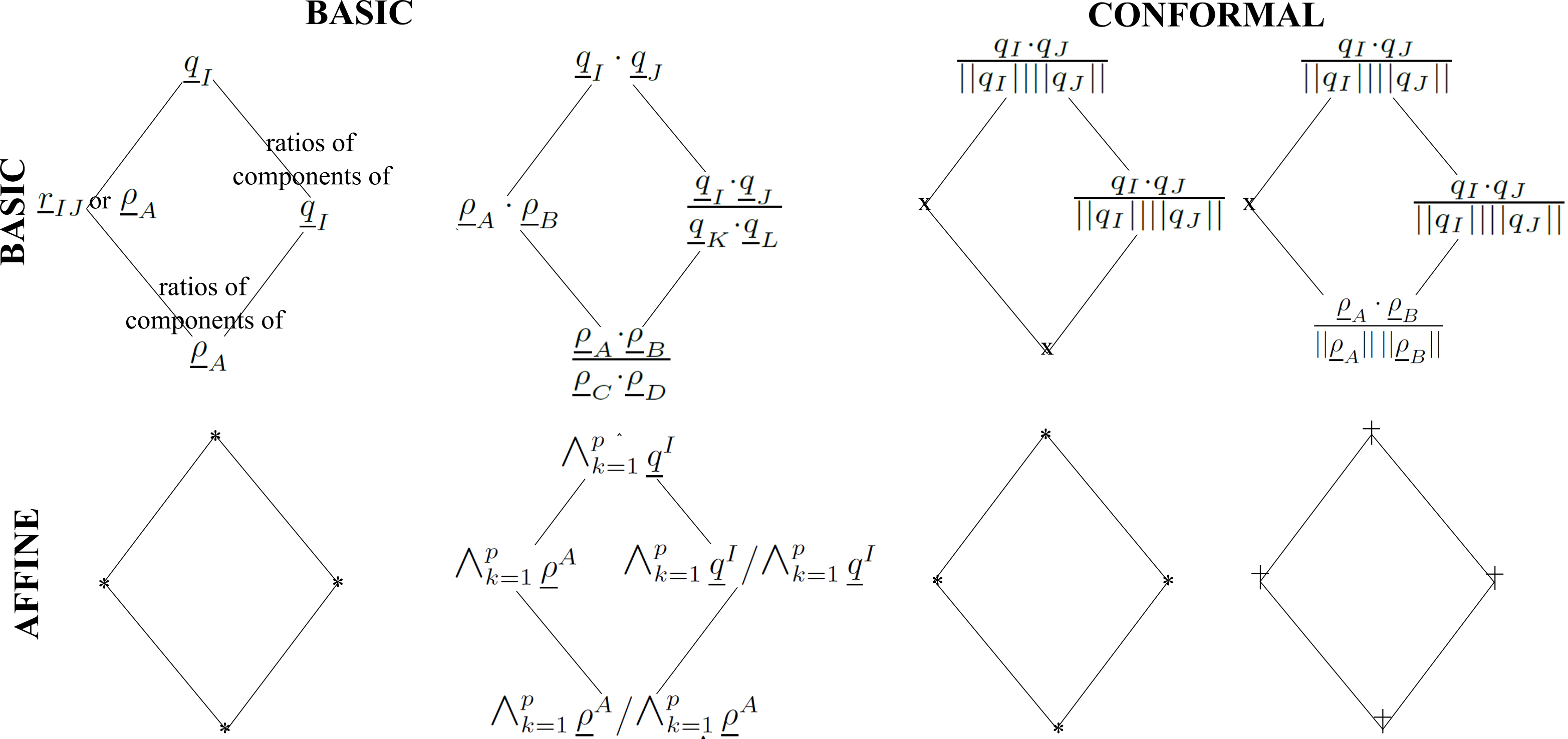
Figure 3: $\mathfrak{g}$-invariants.

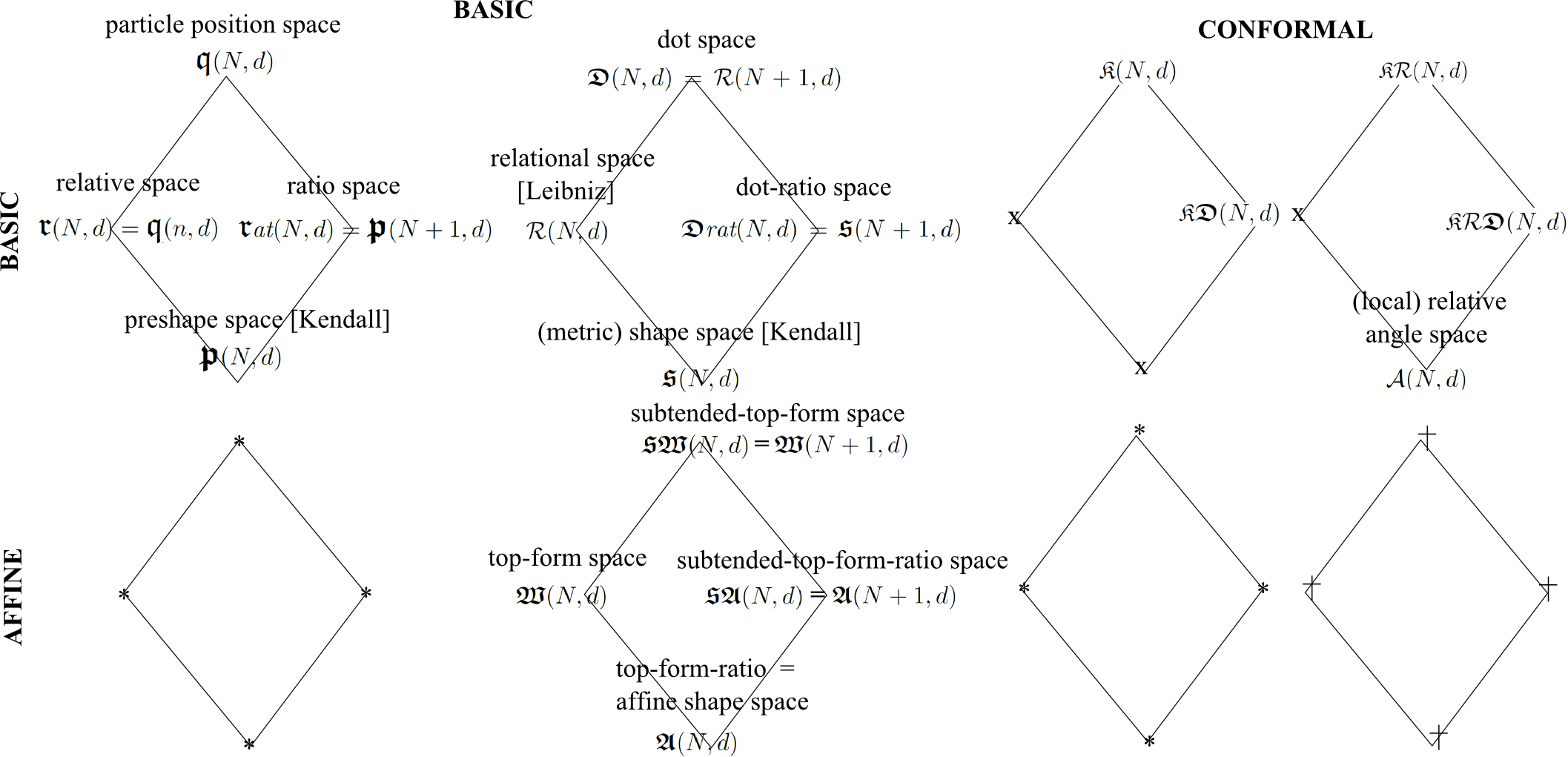
Figure 4: Corresponding relational configuration spaces [13]. Useful inter-relations are also laid out: a number of configuration spaces are the same as others with one particle less by $n$ Jacobi coordinates taking the same mathematical form as $N$ point particle coordinates. ‘Leibniz’ here refers to the relational side [29] of the venerable Absolute versus Relational (Motion) Debate, whereas ‘Kendall’ refers to Kendall’s Shape Theory [24].

Our objective is to consider the theories in Fig 1 corresponding to the geometrically significant groups in Fig 2. The corresponding configuration beables are tabulated in Fig 3, with the corresponding configuration spaces listed in Fig 4.

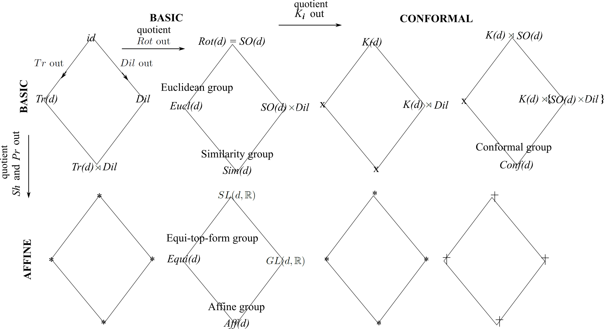
Figure 1: Summary sketch, including further groups acting upon $\mathbb{R}^{d}$ by quotienting. $Tr$ are translations, $Rot$ are rotations, and $Dil$ are dilations. I use $P$, $M$ and $D$ for their generators respectively, alongside $K$ for the special conformal transformations’, $Sh$ for the shears and $Pr$ for the ‘Procrustean stretches’ (The last is a top form preserving stretch, for the top form supported by the dimension in question, e.g. area-preserving in 2-$d$ or volume-preserving in 3-$d$.) Using the abstract Lie group form of brackets, then absences marked $X$ are due to the integrability $\mbox{\bf|[}K\mbox{\bf,}\,P\mbox{\bf]|}\sim D+M$. Absences marked $*$ are due to the integrability $\mbox{\bf|[}Sh\mbox{\bf,}\,Sh\mbox{\bf]|}\sim M$. Finally, absences marked $\dagger$ are due to affine-to-special-conformal obstruction.

Figure 2: Corresponding RPM theories’ names.

1) The zero total momentum constraint is

$$\underline{\mbox{\scriptsize${\cal P}$}}:=\sum\mbox{}_{\mbox{}_{\mbox{\scriptsize$I$=1}}}^{N}\underline{q}^{I}=0\mbox{ }.$$ (5)

The corresponding classical Kuchař beables condition $\mbox{\bf\{}\underline{\mbox{\scriptsize${\cal P}$}}\mbox{\bf,}\,\mbox{\scriptsize$K$}_{\mbox{{\scriptsize K}}}\mbox{\bf\}}\mbox{ }`=^{\prime}\mbox{ }0$ gives the PDE

$$\sum\mbox{}_{\mbox{}_{\mbox{\scriptsize$I$=1}}}^{N}\frac{\partial\mbox{\scriptsize$K$}_{\mbox{{\scriptsize K}}}}{\partial\underline{q}^{I}}\mbox{ }`=^{\prime}\mbox{ }0\mbox{ },$$ (6)

which is solved by the relative interparticle separation vectors and linear combinations thereof. Indeed the latter are often more convenient, in particular the well-known relative Jacobi coordinates $\rho^{A}$ [23] whose interpretation is as relative interparticle cluster separation vectors.

2) The zero total angular momentum constraint is

$$\underline{\mbox{\scriptsize${\cal L}$}}:=\sum\mbox{}_{\mbox{}_{\mbox{\scriptsize$I$=1}}}^{N}\underline{q}^{I}\mbox{\scriptsize{\bf$\mbox{ }\times\mbox{ }$}}\underline{p}_{I}=0$$ (7)

(or the 3-component of this in 2-$d$). The corresponding Kuchař beables condition

$$\mbox{\bf\{}\mbox{\scriptsize${\cal L}$}\mbox{\bf,}\,\mbox{\scriptsize$K$}_{\mbox{{\scriptsize K}}}\mbox{\bf\}}\mbox{ }`=^{\prime}\mbox{ }0$$ (8)

then gives the PDE

$$\sum\mbox{}_{\mbox{}_{\mbox{\scriptsize$I$=1}}}^{N}\left\{\frac{\partial\mbox{\scriptsize$K$}_{\mbox{{\scriptsize K}}}}{\partial\underline{p}^{I}}\mbox{\scriptsize{\bf$\mbox{ }\times\mbox{ }$}}\underline{p_{I}}\mbox{ }\mbox{ }+\mbox{ }\mbox{ }\underline{q}^{I}\mbox{\scriptsize{\bf$\mbox{ }\times\mbox{ }$}}\frac{\partial\mbox{\scriptsize$K$}_{\mbox{{\scriptsize K}}}}{\partial\underline{q}^{I}}\right\}\mbox{ }`=^{\prime}\mbox{ }0\mbox{ }.$$ (9)

This is solved by various dot products. In particular the pure-configurational Kuchař beables equation

$$\sum\mbox{}_{\mbox{}_{\mbox{\scriptsize$I$=1}}}^{N}\underline{q}^{I}\mbox{\scriptsize{\bf$\mbox{ }\times\mbox{ }$}}\frac{\partial\mbox{\scriptsize$K$}_{\mbox{{\scriptsize K}}}}{\partial\underline{q}^{I}}\mbox{ }`=^{\prime}\mbox{ }0$$ (10)

is solved by

$$\underline{q}^{I}\cdot\underline{q}^{J}\mbox{ },$$ (11)

and the pure-momentum Kuchař beables equation

$$\sum\mbox{}_{\mbox{}_{\mbox{\scriptsize$I$=1}}}^{N}\frac{\partial\mbox{\scriptsize$K$}_{\mbox{{\scriptsize K}}}}{\partial\underline{p}_{I}}\mbox{\scriptsize{\bf$\mbox{ }\times\mbox{ }$}}\underline{p}_{I}\mbox{ }`=^{\prime}\mbox{ }0$$ (12)

is solved by

$$\underline{p}^{I}\cdot\underline{p}^{J}$$ (13)

due to $\underline{q}^{I}\leftrightarrow\underline{p}^{I}$ exchange symmetry with the previous equation. The full equation is not solved by $\underline{q}^{I}\cdot\underline{p}^{J}$ but by

$$\underline{q}^{I}\cdot\underline{p}^{J}+\underline{p}^{I}\cdot\underline{q}^{J}\mbox{ },$$ (14)

which is of course the outcome of applying the product rule to $\underline{q}^{I}\cdot\underline{q}^{J}$. Note that norms and angles are particular cases among the above, once the Appendix’s Lemma 1 is taken into account.

The Appendix’s Remark 2 moreover also holds: if (6) and (9) both apply, then the solutions are dots of differences, which is often moreover usefully rephrased as dots of relative Jacobi vectors. These are the Kuchař beables [9] for metric shape-and-scale RPM [19].

3) The zero total dilational momentum constraint is

$$\mbox{\scriptsize${\cal D}$}:=\sum\mbox{}_{\mbox{}_{\mbox{\scriptsize$I$=1}}}^{N}\underline{q}^{I}\cdot\underline{p}_{I}=0\mbox{ }.$$ (15)

The corresponding Kuchař beables condition

$$\mbox{\bf\{}\mbox{\scriptsize${\cal D}$}\mbox{\bf,}\,\mbox{\scriptsize$K$}_{\mbox{{\scriptsize K}}}\mbox{\bf\}}\mbox{ }`=^{\prime}\mbox{ }0$$ (16)

then gives the PDE

$$\sum\mbox{}_{\mbox{}_{\mbox{\scriptsize$I$=1}}}^{N}\left\{\frac{\partial\mbox{\scriptsize$K$}_{\mbox{{\scriptsize K}}}}{\partial\underline{p}^{I}}\cdot\underline{p_{I}}\mbox{ }\mbox{ }+\mbox{ }\mbox{ }\underline{q}^{I}\cdot\frac{\partial\mbox{\scriptsize$K$}_{\mbox{{\scriptsize K}}}}{\partial\underline{q}^{I}}\right\}\mbox{ }`=^{\prime}\mbox{ }0\mbox{ }.$$ (17)

The above can be recognized as an Euler’s homogeneity equation of degree zero, so its solutions are ratios. The pure-configurational Kuchař beables equation is then

$$\sum\mbox{}_{\mbox{}_{\mbox{\scriptsize$I$=1}}}^{N}\underline{q}^{I}\cdot\frac{\partial\mbox{\scriptsize$K$}_{\mbox{{\scriptsize K}}}}{\partial\underline{q}^{I}}\mbox{ }`=^{\prime}\mbox{ }0\mbox{ },$$ (18)

and the pure-momentum Kuchař beables equation is (note the $\underline{q}^{I}\leftrightarrow\underline{p}^{I}$ exchange symmetry again)

$$\sum\mbox{}_{\mbox{}_{\mbox{\scriptsize$I$=1}}}^{N}\frac{\partial\mbox{\scriptsize$K$}_{\mbox{{\scriptsize K}}}}{\partial\underline{p}_{I}}\cdot\underline{p}_{I}\mbox{ }`=^{\prime}\mbox{ }0\mbox{ }.$$ (19)

The Appendix’s composition principle then gives that if (6) and (19) apply, have ratios of differences, if (9) and (19) apply, have ratios of dots, and if all three apply, have ratios of dots of differences. These are the Kuchař beables [9] for metric shape RPM [20]. See [24, 21, 22] for more on metric pure shapes; [25] contains a summary of the corresponding configuration spaces for these, with comparison to those of GR.

4) One further possibility involves a $\mathbb{R}^{d}\longrightarrow\mathbb{S}^{d}$ change of underlying absolute space model. In the case modulo isometries, the constraints are ${\cal L}$ for $\mathbb{S}^{1}$, $\underline{\mbox{\scriptsize${\cal L}$}}$ in $\mathbb{S}^{2}$, and a pair $\underline{\mbox{\scriptsize${\cal L}$}}$, $\underline{\mbox{\scriptsize${\cal L}$}}^{\prime}$ in $\mathbb{S}^{3}$. The unreduced variables are now $\mathbb{S}^{p}$ angles $\theta^{iI}$ rather than particle positions $q^{iI}$ are involved, and there are no $Tr(d)$ or $Dil$. The invariants in this case are the spherical version of the dot product.

5) The RPM on the torus $\mathbb{T}^{n}$ modulo isometries has also been worked out [26, 27].

6) A second branch of further consistent possibilities [13] involves extending the zero total angular momentum constraint to the zero total $SL(d,\mathbb{R})$ momentum constraint

$$\underline{\mbox{\scriptsize${\cal S}$}}:=\sum\mbox{}_{\mbox{}_{\mbox{\scriptsize$I$=1}}}^{N}\underline{q}^{I}\underline{\underline{\underline{S}}}\mbox{ }\underline{p}_{I}\mbox{ }.$$ (20)

E.g. in 2-$d$,

$$\underline{\underline{\underline{S}}}:=\mbox{\Huge[}\mbox{\Huge(}\stackrel{{\scriptstyle\mbox{1 \,\, 0}}}{{\mbox{0 \, --1}}}\mbox{\Huge)},\mbox{\Huge(}\stackrel{{\scriptstyle\mbox{0 \,\, 1}}}{{\mbox{1 \,\,\, 0}}}\mbox{\Huge)},\mbox{\Huge(}\stackrel{{\scriptstyle\mbox{0 \, --1}}}{{\mbox{1 \,\,\, 0}}}\mbox{\Huge)}\mbox{\Huge]}^{\mbox{\scriptsize T}}\mbox{ };$$ (21)

(20) is an area-preserving constraint in this case. In 3-$d$, it is a volume-preserving constraint, and in general it is a top form preserving constraint for the top form corresponding to the dimension in question. Then the classical Kuchař beables condition

$$\mbox{\bf\{}\mbox{\scriptsize${\cal S}$}\mbox{\bf,}\,\mbox{\scriptsize$K$}_{\mbox{{\scriptsize K}}}\mbox{\bf\}}\mbox{ }`=^{\prime}\mbox{ }0$$ (22)

gives the PDE

$$\sum\mbox{}_{\mbox{}_{\mbox{\scriptsize$I$=1}}}^{N}\left\{\frac{\partial\mbox{\scriptsize$K$}_{\mbox{{\scriptsize K}}}}{\partial\underline{p}^{I}}\mbox{ }\underline{\underline{\underline{S}}}\mbox{ }\underline{p_{I}}\mbox{ }\mbox{ }-\mbox{ }\mbox{ }\underline{q}^{I}\mbox{ }\underline{\underline{\underline{S}}}\mbox{ }\frac{\partial\mbox{\scriptsize$K$}_{\mbox{{\scriptsize K}}}}{\partial\underline{q}^{I}}\right\}\mbox{ }`=^{\prime}\mbox{ }0\mbox{ }.$$ (23)

This is solved in 2-$d$ by areas between pairs vectors, in 3-$d$ by volumes of parallelepipeds formed by triples of vectors, and in arbitrary $d$ by the top form supported by that dimension formed by $d$-tuplets of such vectors. The pure-configuration Kuchař beables equation is

$$\sum\mbox{}_{\mbox{}_{\mbox{\scriptsize$I$=1}}}^{N}\underline{q}^{I}\mbox{ }\underline{\underline{\underline{S}}}\mbox{ }\frac{\partial\mbox{\scriptsize$K$}_{\mbox{{\scriptsize K}}}}{\partial\underline{q}^{I}}\mbox{ }`=^{\prime}\mbox{ }0\mbox{ },$$ (24)

and the pure-momentum Kuchař beables equation is

$$\sum\mbox{}_{\mbox{}_{\mbox{\scriptsize$I$=1}}}^{N}\frac{\partial\mbox{\scriptsize$K$}_{\mbox{{\scriptsize K}}}}{\partial\underline{p}^{I}}\mbox{ }\underline{\underline{\underline{S}}}\mbox{ }\underline{p_{I}}\mbox{ }`=^{\prime}\mbox{ }0\mbox{ }$$ (25)

(note $\underline{q}^{I}\leftrightarrow\underline{p}^{I}$ exchange symmetry once again). The Appendix’s composition principle continues to apply here, so we can have top forms of differences, ratios of top forms and ratios of top forms of differences. The last of these corresponds to affine geometry and the first of these to ‘equi-top-form’ geometry (equiareal [28] in 2-$d$).

7) A third branch involves including instead the special conformal transformations This follows from the 19th century observation that inversion in sphere also preserves angles, and well-known in 20th century Theoretical Physics through e.g. Conformal Field Theory (CFT) and its subsequent Particle Physics and String Theory applications. Moreover, this is no longer compatible with trivial removal of translations. In the RPM context, including the special conformal transformations leads to the zero total special conformal constraint [13]

$$\mbox{\scriptsize${\cal K}$}_{a}:=\sum\mbox{}_{\mbox{}_{\mbox{\scriptsize$I$=1}}}^{N}\{q^{I\,2}{\delta_{a}}^{b}-2q^{I}_{a}q^{Ib}\}p_{Ib}=0\mbox{ }.$$ (26)

Additionally, four subgroups including special conformal transformations are indicated in Fig 1. All require the invariants to be angles (special conformal transformation is a strong condition in this regard). The case with $Tr(d)$ as well does use the $\rho^{iA}$ version; the other cases jointly involve the $q^{iI}$ version.

The classical Kuchař beables equation

$$\mbox{\bf\{}\mbox{\scriptsize${\cal K}$}_{a}\mbox{\bf,}\,\mbox{\scriptsize$K$}_{\mbox{{\scriptsize K}}}\mbox{\bf\}}\mbox{ }`=^{\prime}\mbox{ }0$$ (27)

then gives

$$\sum\mbox{}_{\mbox{}_{\mbox{\scriptsize$I$=1}}}^{N}\left\{2\{2\,p_{I[i}q_{j]I}-(\underline{q}\cdot\underline{p})\delta_{ij}\}\frac{\partial\mbox{\scriptsize$K$}_{\mbox{{\scriptsize K}}}}{\partial p_{Ij}}-\{q_{I}^{2}\delta^{ij}-2q^{iI}q^{Ij}\}\frac{\partial\mbox{\scriptsize$K$}_{\mbox{{\scriptsize K}}}}{\partial q^{Ij}}\right\}\mbox{ }`=^{\prime}\mbox{ }0\mbox{ }.$$ (28)

The pure-configuration Kuchař beables equation is

$$\sum\mbox{}_{\mbox{}_{\mbox{\scriptsize$I$=1}}}^{N}\{q_{I}^{2}\delta^{ij}-2\,q^{iI}q^{Ij}\}\frac{\partial\mbox{\scriptsize$K$}_{\mbox{{\scriptsize K}}}}{\partial q^{Ij}}\mbox{ }`=^{\prime}\mbox{ }0\mbox{ }.$$ (29)

The pure-momentum Kuchař beables equation is

$$\sum\mbox{}_{\mbox{}_{\mbox{\scriptsize$I$=1}}}^{N}2\{2\,p_{I[i}q_{j]I}-(\underline{q}^{I}\cdot\underline{p}_{I})\delta_{ij}\}\frac{\partial\mbox{\scriptsize$K$}_{\mbox{{\scriptsize K}}}}{\partial p_{Ij}}\mbox{ }`=^{\prime}\mbox{ }0\mbox{ }$$ (30)

(note that this is no longer symmetric with the previous equation).

Remark 1) In 2-$d$, the full conformal group becomes infinite-dimensional and thus unsuitable for finite RPMs.

Remark 2) One can also consider the sphere versions of stripping away further layers of geometrical structure, though I leave this matter for a future occasion.

Dirac beables equations for the theories involving whichever subgroup-forming combination of ${\cal P}$, ${\cal L}$, ${\cal D}$ and ${\cal K}$ the following extra equation.

$$0\mbox{ }`=^{\prime}\mbox{ }\mbox{\bf\{}\mbox{\scriptsize${\cal E}$}\mbox{\bf,}\,\mbox{\scriptsize$D$}_{\mbox{{\scriptsize D}}}\mbox{\bf\}}=\sum\mbox{}_{\mbox{}_{\mbox{\scriptsize$I$=1}}}^{N}\left\{\frac{\partial V}{\partial q^{I}}\frac{\partial\mbox{\scriptsize$D$}_{\mbox{{\scriptsize D}}}}{\partial p_{I}}-p_{I}\frac{\partial\mbox{\scriptsize$D$}_{\mbox{{\scriptsize D}}}}{\partial q^{I}}\right\}\mbox{ }.$$ (31)

A distinct equation is required in the other cases. E.g. the equiareal and 2-$d$ affine cases each require distinct ${\cal E}$’s built from cross-products rather than from Euclidean norms.

3 Gauge Theory beables or observables

For Electromagnetism, which has the Gauss constraint

$$\mbox{{\scriptsize G}}:=\underline{\partial}\cdot\underline{\pi}\mbox{ },$$ (32)

the classical Kuchař beables condition

$$\mbox{\bf\{}(\mbox{\scriptsize${\cal G}$}|\xi)\mbox{\bf,}\,(\mbox{\scriptsize$K$}_{\mbox{{\scriptsize K}}}|\chi^{\mbox{{\scriptsize K}}})\mbox{\bf\}}\mbox{ }`=^{\prime}\mbox{ }0$$ (33)

(for smearing functions $\xi$ and $\chi^{\mbox{{\scriptsize K}}}$) gives the FDE

$$\underline{\partial}\cdot\frac{\delta\mbox{\scriptsize$K$}_{\mbox{{\scriptsize K}}}}{\delta\underline{\mbox{A}}}\mbox{ }`=^{\prime}\mbox{ }0\mbox{ }.$$ (34)

This is solved by $\underline{\mbox{E}}$ and $\underline{\mbox{B}}=\underline{\partial}\mbox{\scriptsize{\bf$\mbox{ }\times\mbox{ }$}}\underline{\mbox{A}}$, and thus by a functional

$${\cal F}[\underline{\mbox{B}},\,\underline{\mbox{E}}]$$ (35)

by Lemma 1 in the Appendix. We can also write this in an integrated version in terms of fluxes:

$${\cal F}\left[\iint_{S}\underline{\mbox{B}}\cdot\textrm{d}\underline{S},\iint_{S}\underline{\mbox{E}}\cdot\textrm{d}\underline{S}\right]={\cal F}[W_{\gamma},\Phi_{S}^{\mbox{\scriptsize E}}]$$ (36)

for electric flux $\Phi_{S}^{\mbox{\scriptsize E}}$ and loop variable

$$W_{\gamma}:=\mbox{exp}\left(\oint_{\gamma}\underline{\mbox{A}}\cdot\textrm{d}\underline{\mbox{l}}\right)\mbox{ }.$$ (37)

This is by use of Stokes’ Theorem with $\gamma:=\partial S$ and then insertion of the exponentiation function subcase of Lemma 1 (this ties the construct to the geometrical notion of holonomy).

All of the above carries over to Yang–Mills theory as well. This has the Yang–Mills–Gauss constraint

$${\mbox{\scriptsize${\cal G}$}}_{J}:=\mbox{D}_{a}\uppi^{a}_{J}=\partial_{a}\uppi^{a}_{J}-\mbox{\mbox{g}}f_{IJK}\mbox{A}^{K}_{a}\pi^{Ia}=0\mbox{ }.$$ (38)

The classical Kuchař beables condition

$$\mbox{\bf\{}(\mbox{\scriptsize${\cal G}$}_{I}|\xi^{I})\mbox{\bf,}\,(\mbox{\scriptsize$K$}_{\mbox{{\scriptsize K}}}|\chi^{\mbox{{\scriptsize K}}})\mbox{\bf\}}\approx 0$$ (39)

gives

$$\underline{\mbox{D}_{a}}\cdot\frac{\delta\mbox{\scriptsize$K$}_{\mbox{{\scriptsize K}}}}{\delta\mbox{A}_{aJ}}\approx 0\mbox{ },$$ (40)

which is solved by $\underline{\mbox{E}}_{I}$ and $\underline{\mbox{B}}_{I}$, so

$${\cal F}[\underline{\mbox{E}}_{I},\,\underline{\mbox{B}}_{I}]$$ (41)

solves as well by Lemma 1. Once again, this can be rewritten as

$${\cal F}[W_{\gamma},\Phi_{S}^{\mbox{\scriptsize E}}]\mbox{ },$$ (42)

now for loop variable [30]

$$W(\gamma):=\mbox{Tr}\left(P\,\mbox{exp}\left(i\mbox{g}\oint_{\gamma}\textrm{d}x^{i}\mbox{A}_{iP}(x)\mbox{g}^{P}(x)\right)\right)\mbox{ }.$$ (43)

4 GR beables or observables

For GR-as-geometrodynamics [31], the linear GR momentum constraint is

$$\mbox{\scriptsize${\cal M}$}_{i}=-2\,\mbox{D}_{j}{\mbox{p}^{j}}_{i}=0\mbox{ }.$$ (44)

The corresponding Kuchař beables condition is then

$$\mbox{\bf\{}(\mbox{\scriptsize${\cal M}$}_{i}|\mbox{L}^{i})\mbox{\bf,}\,(\mbox{\scriptsize$K$}_{\mbox{{\scriptsize K}}}|\chi^{\mbox{{\scriptsize K}}})\mbox{\bf\}}=\left(\left\{\pounds_{\mbox{\scriptsize L}}\mbox{h}_{ij}\,\frac{\delta}{\delta\mbox{h}_{ij}}+\pounds_{\mbox{\scriptsize L}}\mbox{p}^{ij}\,\frac{\delta}{\delta\mbox{p}^{ij}}\right\}\mbox{\scriptsize$K$}_{\mbox{{\scriptsize K}}}\,\mbox{\Huge|}\,\chi^{\mbox{{\scriptsize K}}}\right)\mbox{ }`=^{\prime}\mbox{ }0\mbox{ },$$ (45)

which corresponds to the unsmeared FDE

$$2\,\mbox{h}_{jk}\mbox{D}_{i}\frac{\delta\mbox{\scriptsize$K$}_{\mbox{{\scriptsize K}}}}{\delta\mbox{h}_{ij}}+\big{\{}\mbox{D}_{i}\mbox{p}^{lj}-2{\delta^{j}}_{i}\{\mbox{D}_{e}\mbox{p}^{le}+\mbox{p}^{le}\mbox{D}_{e}\}\big{\}}\,\frac{\delta\mbox{\scriptsize$K$}_{\mbox{{\scriptsize K}}}}{\delta\mbox{p}^{lj}}\mbox{ }`=^{\prime}\mbox{ }0\mbox{ }.$$ (46)

In the weak case, we can furthermore discard the penultimate term. Then the purely configurational solutions of

$$2\,\mbox{h}_{jk}\mbox{D}_{i}\frac{\delta\mbox{\scriptsize$K$}_{\mbox{{\scriptsize K}}}}{\delta\mbox{h}_{ij}}\mbox{ }`=^{\prime}\mbox{ }0\mbox{ }$$ (47)

are 3-geometry quantities ‘${\mbox{\boldmath$\mathfrak{G}$}}^{(3)}$’ by (47) emulating (and moreover logically preceding) the quantum momentum constraint,

$$2\,\mbox{h}_{jk}\mbox{D}_{i}\frac{\delta\Psi}{\delta\mbox{h}_{ij}}=0$$ (48)

[32]. Moreover, explicit ‘basis beables’ (see the Appendix) are not known in this case.

On the other hand, the complementary part of this gives a FDE for the associated 3-geometry momenta ‘$\Pi^{\mbox{\boldmath\scriptsize$\mathfrak{G}$}^{(3)}}$’. These formal entities solve the the GR momentum beables equation

$$\big{\{}\mbox{D}_{i}\mbox{p}^{lj}-2\,{\delta^{j}}_{i}\{\mbox{D}_{e}\mbox{p}^{le}+\mbox{p}^{le}\mbox{D}_{e}\}\big{\}}\,\frac{\delta\mbox{\scriptsize$K$}_{\mbox{{\scriptsize K}}}}{\delta\mbox{p}^{lj}}\mbox{ }`=^{\prime}\mbox{ }0\mbox{ }.$$ (49)

N.B. that GR also has a quadratic Hamiltonian constraint

$$\mbox{\scriptsize${\cal H}$}:=\mbox{N}_{ijkl}\mbox{p}^{ij}\mbox{p}^{kl}-\sqrt{\mbox{h}}\{\mbox{R}-2\Lambda\}$$ (50)

Here

$$\mbox{M}^{abcd}:=\sqrt{\mbox{h}}\{\mbox{h}^{ac}\mbox{h}^{bd}-\mbox{h}^{ab}\mbox{h}^{cd}\}$$ (51)

is the GR kinetic metric, and

$$\mbox{N}_{abcd}:=\{\mbox{h}_{ac}\mbox{h}_{bd}-\mbox{h}_{ab}\mbox{h}_{cd}/2\}/\sqrt{\mbox{h}}$$ (52)

is its inverse the DeWitt supermetric [33]. Moreover, under the DeWitt 2-index to 1-index map [33],

$$\mbox{h}_{ab}\mbox{ }\longrightarrow\mbox{ }\mbox{h}^{A}\mbox{ }\mbox{ and }\mbox{ }\mbox{p}^{ab}\mbox{ }\longrightarrow\mbox{ }\mbox{p}_{A}\mbox{ },$$ (53)

$$\mbox{M}^{abcd}\mbox{ }\mbox{ becomes manifestly a metric }\mbox{ }\mbox{M}_{AB}$$ (54)

and

$$\mbox{N}_{abcd}\mbox{ }\mbox{ becomes }\mbox{ }\mbox{N}^{AB}\mbox{ }.$$ (55)

Thus Dirac beables or observables for geometrodynamics require extra equation

$$\mbox{\bf\{}(\mbox{\scriptsize${\cal H}$}|\mbox{J})\mbox{\bf,}\,(\mbox{\scriptsize$D$}_{\mbox{{\scriptsize D}}}|\chi^{\mbox{{\scriptsize D}}})\mbox{\bf\}}\mbox{ }`=^{\prime}\mbox{ }0\mbox{ },$$ (56)

which gives

$$\left(\left\{\frac{\delta\mbox{\scriptsize$D$}_{\mbox{{\scriptsize D}}}}{\delta\underline{\mbox{p}}}\left\{\underline{\mbox{G}}-\underline{\underline{\mbox{M}}}\,\underline{\mbox{D}}^{2}\right\}-\frac{\delta\mbox{\scriptsize$D$}_{\mbox{{\scriptsize D}}}}{\delta\underline{\mbox{h}}}\,\underline{\underline{\mbox{N}}}\mbox{ }\underline{\mbox{p}}\right\}\mbox{L}\mbox{\Huge|}\chi^{\mbox{{\scriptsize D}}}\right)$$ (57)

for DeWitt vector quantities

$$\underline{\mbox{G}}:=\mbox{$\frac{2}{\sqrt{\mbox{\scriptsize h}}}$}\big{\{}\mbox{p}^{ia}{\mbox{p}_{a}}^{j}-\mbox{$\frac{\mbox{\scriptsize p}}{2}$}\mbox{p}^{ij}\big{\}}-\mbox{$\frac{1}{2\sqrt{\mbox{\scriptsize h}}}$}\big{\{}\mbox{p}^{ab}\mbox{p}_{ab}-\mbox{$\frac{\mbox{\scriptsize p}^{2}}{2}$}\big{\}}\mbox{h}^{ij}-\mbox{$\frac{\sqrt{\mbox{\scriptsize h}}}{2}$}\big{\{}\mbox{h}_{ij}\mbox{R}-2\,\mbox{R}^{ij}\big{\}}+\sqrt{\mbox{h}}\,\Lambda\,\mbox{h}^{ij}$$ (58)

familiar from ADM evolution [31] and

$$\underline{\mbox{D}}^{2}:=\mbox{D}^{i}\mbox{D}^{j}\mbox{ }.$$ (59)

In unsmeared form, (57) is the FDE

$$\{\underline{\mbox{G}}-\underline{\underline{\mbox{M}}}\mbox{ }\underline{\mbox{D}}^{2}\}\frac{\delta\mbox{\scriptsize$D$}_{\mbox{{\scriptsize D}}}}{\delta\underline{\mbox{p}}}\mbox{ }`=^{\prime}\mbox{ }2\,\underline{\mbox{p}}\mbox{ }\underline{\underline{\mbox{N}}}\mbox{ }\frac{\delta\mbox{\scriptsize$D$}_{\mbox{{\scriptsize D}}}}{\delta\underline{\mbox{h}}}\mbox{ }.$$ (60)

Some examples of Dirac observables in GR for more specialized highly symmetric cases can be found in e.g. [34, 35, 36].

Acknowledgments To those close to me gave me the spirit to do this. Thanks also to Chris Isham, Malcolm MacCallum, Jeremy Butterfield, Don Page, Enrique Alvarez and the Foundational Questions Institute.

Appendix A Supporting Lemmas

Lemma 1. If $\mbox{\scriptsize$B$}_{\mbox{{\scriptsize B}}}$ are beables, then so are the functionals ${\cal F}[\mbox{\scriptsize$B$}_{\mbox{{\scriptsize B}}}]$.

Proof. For $L$ linear, if $u$ solves

$$L\phi\mbox{ }`=^{\prime}\mbox{ }0\mbox{ },$$ (61)

then $f(u)$ and $F[u]$ also solve this equation by the chain-rule. Then indeed, the PDE or FDE for the beables is an equation of this form.

Remark 1) This renders ‘basis beables’ a useful concept: i.e. a sufficient set of Kuchař beables to describe one’s theory by $K_{\mbox{{\scriptsize K}}}$. These are a mutually functionally independent choice of

$$\mbox{dim(reduced phase space)}=2\,q-c$$ (62)

reduced phase space quantities (for $q=\mbox{dim}(\mbox{\Large$\mathfrak{q}$})$ and $c$ the amount of phase space degrees of freedom taken out by the constraints). This is $2\{q-g\}$ in the simplest case of $g$ first-class constraints alone. See e.g. [21, 22] for RPM examples of ‘basis beables’.

Remark 2) (Composition Principle) In the case of multiple functional dependency restrictions applying, the composition of these restrictions applies; see Sec 2 for examples.

Lemma 2. The pure-configuration Kuchař beables equation is the same as the equation determining which quantities are annihilated by the generators.

Remark 3) This refers to the configuration space $\mathfrak{q}$ uplift of the group generators acting upon absolute space $\mathfrak{a}$, by which one passes from $\mathfrak{a}$-invariants to ones built out of multiple particle positions $q^{iI}$.

Proof. This occurs since the constraints involved are homogeneous linear in $p_{iI}$, so the Poisson bracket removes the $p_{iI}$ factors and replaces them with $\partial/\partial q^{iI}$ factors. [The Poisson bracket term with the other sign is annihilated by the pure-configuration restriction.]

Remark 4) The pure-momentum case of Kuchař beables has no such result as constraints are not confined to be linear in the $Q^{A}$. Those that are double-linear have pure-$P_{\mbox{{\scriptsize A}}}$ and pure-$Q^{\mbox{{\scriptsize A}}}$ beables close parallel. On the other hand, those which are not have more divergence between the forms of these two contributions to the ‘basis beables’.

References

[1]
[2] P.A.M. Dirac, Lectures on Quantum Mechanics (Yeshiva University, New York 1964).
[3] M. Henneaux and C. Teitelboim, Quantization of Gauge Systems (Princeton University Press, Princeton 1992).
[4] E. Anderson, “The Problem of Time. General Relativity versus Quantum Mechanics", (Springer, 2017).
[5] J. Śniatycki, “Dirac Brackets in Geometric Dynamics", Ann. Inst. H. Poincaré 20 365 (1974).
[6] P.A.M. Dirac, Rev. Mod. Phys. 21 392 (1949).
[7] K.V. Kuchař, in Proceedings of the 4th Canadian Conference on
General Relativity and Relativistic Astrophysics ed. G. Kunstatter, D. Vincent and J. Williams (World Scientific, Singapore, 1992).
Reprinted as Int. J. Mod. Phys. Proc. Suppl. D20 3 (2011);
C.J. Isham, in Integrable Systems, Quantum Groups and Quantum Field Theories
ed. L.A. Ibort and M.A. Rodríguez (Kluwer, Dordrecht 1993), gr-qc/9210011.
[8] K.V. Kuchař, in General Relativity and Gravitation 1992,
ed. R.J. Gleiser, C.N. Kozamah and O.M. Moreschi M (Institute of Physics Publishing, Bristol 1993), gr-qc/9304012.
[9] E. Anderson, SIGMA 10 092 (2014), arXiv:1312.6073.
[10] E. Anderson, arXiv:1809.02045.
[11] E. Anderson, arXiv:1809.07738.
[12] E. Anderson, arXiv:1411.4316.
[13] E. Anderson, Int. J. Mod. Phys. D 25 1650044 (2016), arXiv:1505.00488.
[14] B. Dittrich, Gen. Rel. Grav. 38 1891 (2007), gr-qc/0411013;
Class. Quant. Grav. 23 6155 (2006), gr-qc/0507106;
T. Thiemann, Modern Canonical Quantum General Relativity (Cambridge University Press, Cambridge 2007);
J. Tambornino, SIGMA 8 017 (2012), arXiv:1109.0740.
[15] E. Anderson, Annalen der Physik, 524 757 (2012), arXiv:1206.2403;
arXiv:1409.4117;
Chapters 9, 10 and 12 of [4].
[16] I.A. Batalin and I.V. Tyutin, Int. J. Mod. Phys A6 3255 (1991).
[17] E. Anderson and F. Mercati, arXiv:1311.6541;
E. Anderson, arXiv:1501.07822;
Appendix L of [4].
[18] E. Anderson, arXiv:1505.02448.
[19] J.B. Barbour and B. Bertotti, Proc. Roy. Soc. Lond. A382 295 (1982).
[22] E. Anderson, Int. J. Mod. Phys. D23 1450014 (2014), arXiv:1202.4186.
[23] See e.g. C. Marchal, Celestial Mechanics (Elsevier, Tokyo 1990).
[24] D.G. Kendall, D. Barden, T.K. Carne and H. Le, Shape and Shape Theory (Wiley, Chichester 1999).
[25] E. Anderson, arXiv:1503.01507;
Appendices G, H, I and N of [4].
[26] E. Anderson, arxiv:1811.06516.
[27] E. Anderson, “Shapes on the Torus", forthcoming December 2018.
[28] H.S.M. Coxeter, Introduction to Geometry (Wiley, New York 1989).
[29] See The Leibnitz–Clark Correspondence, ed. H.G. Alexander (Manchester University Press, Manchester 1956).
[30] R. Gambini and J. Pullin Loops, Knots, Gauge Theories and Quantum Gravity (Cambridge University Press, Cambridge 1996).
[31] R. Arnowitt, S. Deser and C.W. Misner,
in Gravitation: An Introduction to Current Research ed. L. Witten (Wiley, New York 1962), arXiv:gr-qc/0405109.
[32] J.A. Wheeler, in Battelle Rencontres: 1967 Lectures in Mathematics and Physics ed. C. DeWitt and J.A. Wheeler (Benjamin, New York 1968).