The Directed Dominating Set Problem: Generalized Leaf Removal and Belief Propagation

Abstract

A minimum dominating set for a digraph (directed graph) is a smallest set of vertices such that each vertex either belongs to this set or has at least one parent vertex in this set. We solve this hard combinatorial optimization problem approximately by a local algorithm of generalized leaf removal and by a message-passing algorithm of belief propagation. These algorithms can construct near-optimal dominating sets or even exact minimum dominating sets for random digraphs and also for real-world digraph instances. We further develop a core percolation theory and a replica-symmetric spin glass theory for this problem. Our algorithmic and theoretical results may facilitate applications of dominating sets to various network problems involving directed interactions.

1 Introduction

The construction of a minimum dominating set (MDS) for a general digraph (directed graph) [1, 2] is a fundamental nondeterministic polynomial-hard (NP-hard) combinatorial optimization problem [3]. A digraph $D=\{V,A\}$ is formed by a set $V\equiv\{1,2,..,N\}$ of $N$ vertices and a set $A\equiv\{(i,j):i,j\in V\}$ of $M$ arcs (directed edges), each arc $(i,j)$ pointing from a parent vertex (predecessor) $i$ to a child vertex (successor) $j$. The arc density $\alpha$ is defined simply as $\alpha\equiv M/N$. Each vertex $i$ of digraph $D$ brings a constraint requiring that either $i$ belongs to a vertex set $\Gamma$ or at least one of its predecessors belongs to $\Gamma$. A dominating set $\Gamma$ is therefore a vertex set which satisfies all the $N$ vertex constraints, and the dominating set problem can be regarded as a special case of the more general hitting set problem [4, 5].

A dominating set containing the smallest number of vertices is a MDS, which might not necessarily be unique for a digraph $D$. As a MDS is a smallest set of vertices which has directed edges to all the other vertices of a given digraph, it is conceptually and practically important for analyzing, monitoring, and controlling many directed interaction processes in complex networked systems, such as infectious disease spreading [6], genetic regulation [7, 8], chemical reaction and metabolic regulation [9], and power generation and transportation [10]. Previous heuristic algorithms on the directed MDS problem all came from the computer science/applied mathematics communities [2] and they are based on vertices’ local properties such as in- and out-degrees [11, 6, 12]. In the present work we study the directed MDS problem through statistical mechanical approaches.

In the next section we introduce a generalized leaf-removal (GLR) process to simplify an input digraph $D$. If GLR reduces the original digraph $D$ into an empty one, it then succeeds in constructing an exact MDS. If a core is left behind, we implement a hybrid algorithm combining GLR with an impact-based greedy process to search for near-optimal dominating sets (see Fig. 3 and Table 1). We also study the GLR-induced core percolation by a mean field theory (see Fig. 2). In Sec. 3 we introduce a spin glass model for the directed MDS problem and obtain a belief-propagation decimation (BPD) algorithm based on the replica-symmetric mean field theory. By comparing with ensemble-averaged theoretical results, we demonstrate that the message-passing BPD algorithm has excellent performance on random digraphs and real-world network instances, and it outperforms the local hybrid algorithm (Fig. 3 and Table 1).

This paper is a continuation of our earlier effort [13] which studied the undirected MDS problem. Since each undirected edge between two vertices $i$ and $j$ can be treated as two opposite-direction arcs $(i,j)$ and $(j,i)$, the methods of this paper are more general and they are applicable to graphs with both directed and undirected edges. The algorithmic and theoretical results presented here and in [13] may promote the application of dominating sets to various network problems involving directed and undirected interactions.

In the remainder of this paper, we denote by $\partial i^{+}$ the set of predecessors of a vertex $i$, and refer to the size of this set as the in-degree of $i$; similarly $\partial i^{-}$ denotes the set of successors of vertex $i$ and its size defines the out-degree of this vertex. With respective to a dominating set $\Gamma$, if vertex $i$ belongs to this set, we say $i$ is occupied, otherwise it is unoccupied (empty). If vertex $i$ belongs to the dominating set $\Gamma$ or at least one of its predecessors belongs to $\Gamma$, then we say $i$ is observed, otherwise it is unobserved.

2 Generalized Leaf Removal and the Hybrid Algorithm

The leaf-removal process was initially applied in the vertex-cover problem [14]. It causes a core percolation phase transition in random undirected or directed graphs [15]. Here we consider a generalized leaf-removal process for the directed MDS problem. This GLR process iteratively deletes vertices and arcs from an input digraph $D$ starting from all the $N$ vertices being unoccupied (and unobserved) and the dominating set $\Gamma$ being empty. The microscopic rules of digraph simplification are as follows:

Rule $1$: If an unobserved vertex $i$ has no predecessor in the current digraph $D$, it is added to set $\Gamma$ and become occupied (see Fig. 1A). All the previously unobserved successors of $i$ then become observed.

Rule $2$: If an unobserved vertex $j$ has only a single unoccupied predecessor (say vertex $k$) and no unobserved successor in the current digraph $D$, vertex $k$ is added to set $\Gamma$ and become occupied (Fig. 1B). All the previously unobserved successors of $k$ (including $j$) then become observed.

Rule $3$: If an unoccupied but observed vertex $l$ has only a single unobserved successor (say $m$) in the current digraph $D$, occupying $l$ is not better than occupying $m$, therefore the arc $(l,m)$ is deleted from $D$ (Fig. 1C). We emphasize that vertex $m$ is still unobserved after this arc deletion. (Rule $3$ is specific to the dominating set problem and it is absent in the conventional leaf-removal process [14, 15].)

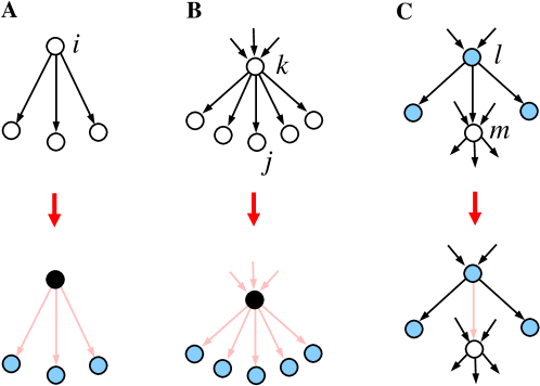
Figure 1: The generalized leaf-removal process. White circles represent unobserved vertices, black circles are occupied vertices, and blue (gray) circles are observed but unoccupied vertices. Pink (light gray) arrows represent deleted arcs, while black arrows are arcs that are still present in the digraph. (A) vertex $i$ has no predecessor, so it is occupied. (B) vertex $j$ has only one predecessor $k$ and no successor, so vertex $k$ is occupied. (C) vertex $l$ has only a single unobserved successor $m$, so the arc $(l,m)$ is deleted.

The above-mentioned microscopic rules only involve the local structure of the digraph, they are simple to implement. Following the same line of reasoning in [13], we can prove that if all the vertices are observed after the GLR process, the constructed vertex set $\Gamma$ must be a MDS for the original digraph $D$. If some vertices remain to be unobserved after the GLR process, this set of remaining vertices is unique and is independent of the particular order of the GLR process.

2.1 Core percolation transition

We apply GLR on a set of random Erdös-Rényi (ER) digraphs and random regular (RR) digraphs (see Fig. 2) and also on a set of real-world directed networks (see Table 1). To generate an ER digraph of size $N$ and arc density $\alpha$, we first select $\alpha N$ different pairs of vertices totally at random from the set of $N(N-1)/2$ possible pairs, and then create an arc of random direction between each selected vertex pair. Similarly, to generate a RR digraph, we first generate an undirected RR graph with every vertex having the same integer number ($=2\alpha$) of edges [13], and then randomly specify a direction for each undirected edge.

If the arc density $\alpha$ of an ER digraph is less than $1.852$ and that of a RR digraph is less than $2.0$, a MDS can be constructed by applying GLR alone. However, if $\alpha>1.852$ for an ER digraph and $\alpha\geq 2.0$ for a RR digraph, GLR only constructs a partial dominating set for the digraph, and a fraction $n_{core}$ of vertices remain to be unobserved after the termination of GLR. For ER digraphs $n_{core}$ increases continuously from zero as $\alpha$ exceeds $1.852$. The sub-digraph induced by all these unobserved vertices and all their predecessor vertices is referred to as the core of digraph $D$.

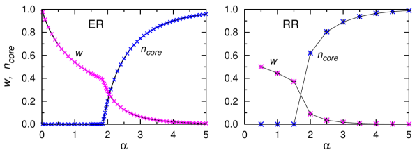
Figure 2: GLR-induced core percolation transition in Erdös-Rényi (left panel) and regular random (right panel) digraphs. $w$ is the fraction of occupied vertices, $n_{core}$ is the fraction of remaining unobserved vertices. Cross symbols are results obtained on a single digraph with $N=10^{6}$ vertices and $M=\alpha N$ arcs, lines (left panel) and plus symbols connected by lines (right panel) are mean-field theoretical results for $N=\infty$.

We develop a percolation theory to quantitatively understand the GLR dynamics on random digraphs. For theoretical simplicity we consider a GLR process carried out in discrete time steps $t=0,1,\ldots$. In each time step $t$, first Rule $1$ is applied to all the eligible vertices, then Rule $2$ is applied to all the eligible vertices, then Rule $3$ is applied to all the eligible arcs, and finally all the newly occupied vertices and their attached arcs are all deleted from digraph $D$. The fraction $w$ of occupied vertices during the whole GLR process and the fraction $n_{core}$ of remaining unobserved vertices are quantitatively predicted by this mean-field theory (see the Appendix for technical details). These theoretical predictions are in complete agreement with simulation results on single digraph instances (Fig. 2). We believe that when there is no core ($n_{core}=0$), the MDS relative size $w$ as predicted by our theory is the exact ensemble-averaged result for finite-connectivity random digraphs.

2.2 The hybrid algorithm

The GLR process can not construct a MDS for the whole digraph $D$ if it contains a core. For such a difficult case we combine GLR with a simple greedy process to construct a dominating set that is not necessarily a MDS. We define the impact of an unoccupied vertex as the number of newly observed vertices caused by occupying this vertex [2, 6, 12]. For example, an unobserved vertex with three unobserved successors has impact $4$, while an observed vertex with three unobserved successors has impact $3$. Our hybrid algorithm has two modes, the default mode and the greedy mode. In the default mode, the digraph is iteratively simplified by occupying vertices according to the microscopic rules of GLR. If there are still unobserved vertices after this process, the algorithm first switches to the greedy mode, in which the digraph is simplified by occupying a vertex randomly chosen from the subset of highest-impact vertices, and then switches back to the default mode.

Table 1: Constructing dominating sets for several real-world network instances containing $N$ vertices and $M=\alpha N$ arcs. For each graph, we list the number of unobserved vertices after the GLR process (Core), the size of the dominating set obtained by a single running of the greedy algorithm (Greedy), the hybrid algorithm (Hybrid), and the BPD algorithm at fixed re-weighting parameter $x=8.0$ (BPD). Epinions1 [16] and WikiVote [17, 18] are two social networks, Email [19] and WikiTalk [17, 18] are two communication networks, HepPh and HepTh [20] are two research citation networks, Google and Stanford [21] are two webpage connection networks, and Gnutella31 [22] is a peer-to-peer network.

Network	$N$	$M$	$\alpha$	Core	Greedy	Hybrid	BPD
Epinions1	$75879$	$405740$	$5.347$	$348$	$37172$	$37128$	$37127$
WikiVote	$7115$	$100762$	$14.162$	$7$	$4786$	$4784$	$4784$
Email	$265214$	$364481$	$1.374$	$0$	$203980$	$203980$	$203980$
WikiTalk	$2394385$	$4659565$	$1.946$	$72$	$63617$	$63614$	$63614$
HepPh	$34546$	$420877$	$12.183$	$982$	$9628$	$9518$	$9512$
HepTh	$27770$	$352285$	$12.686$	$1900$	$7302$	$7213$	$7203$
Google	$875713$	$4322051$	$4.935$	$98473$	$315585$	$314201$	$313986$
Stanford	$281903$	$1992636$	$7.069$	$68947$	$90403$	$89388$	$89466$
Gnutella31	$62586$	$147892$	$2.363$	$26$	$12939$	$12784$	$12784$

The hybrid algorithm can be regarded as an extension of the pure greedy algorithm which always works in the greedy mode. The simulation results obtained by the hybrid algorithm and the pure greedy algorithm are shown in Fig. 3 for random digraphs and in Table 1 for real-world network instances. The hybrid algorithm improves over the greedy algorithm considerably on random digraph instances when the arc density $\alpha\leq 10$. But when the relative size $n_{core}$ of the core in the digraph is close to $1$, the hybrid algorithm only slightly outperforms the pure greedy algorithm.

3 Spin Glass Model and Belief-Propagation

We now introduce a spin glass model for the directed MDS problem and solve it by the replica-symmetric mean field theory, which is based on the Bethe-Peierls approximation [23, 24] but can also be derived without any physical assumptions through partition function expansion [25, 26]. We define a partition function $Z(x)$ for a given input digraph $D$ as follows:

$$Z(x)=\sum\limits_{\underline{c}}\prod\limits_{i\in V}\Bigl{[}e^{-xc_{i}}\bigl{(}1-(1-c_{i})\prod\limits_{j\in\partial i^{+}}(1-c_{j})\bigr{)}\Bigr{]}\;.$$ (1)

The summation in this expression is over all the microscopic configurations $\underline{c}\equiv\{c_{1},c_{2},...,c_{N}\}$ of the $N$ vertices, with $c_{i}\in\{0,1\}$ being the state of vertex $i$ ($c_{i}=0$, empty; $c_{i}=1$, occupied). A configuration $\underline{c}$ has zero contribution to $Z(x)$ if it does not satisfy all the vertex constraints; if it does satisfy all these constraints and therefore is equivalent to a dominating set, it contributes a statistical weight $e^{-xW(\underline{c})}$, with $W(\underline{c})\equiv\sum_{i\in V}c_{i}$ being the total number of occupied vertices. When the positive re-weighting parameter $x$ is sufficiently large, $Z(x)$ will be overwhelmingly contributed by the MDS configurations.

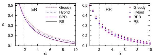
Figure 3: Relative sizes $w$ of dominating sets for Erdös-Rényi (left panel) and random regular (right panel) digraphs. We compare the mean sizes of $96$ dominating sets obtained by the Greedy, the Hybrid, and the BPD algorithm on $96$ digraph instances of size $N=10^{5}$ and arc density $\alpha$ (fluctuations to the mean are of order $10^{-4}$ and are not shown). The MDS relative sizes predicted by the replica-symmetric theory are also shown. The re-weighting parameter is fixed to $x=10.0$ for ER digraphs and to $x=8.0$ for RR digraphs. The vertical dashed lines mark the core-percolation transition point $\alpha\approx 1.852$ for ER digraphs and $\alpha=2.0$ for RR digraphs.

We define on each arc $(i,j)$ of digraph $D$ a distribution function $q_{i\rightarrow j}^{c_{i},c_{j}}$, which is the probability of vertex $i$ being in state $c_{i}$ and vertex $j$ being in state $c_{j}$ if all the other attached arcs of $j$ are deleted and the constraint of $j$ is relaxed, and another distribution function $q_{j\leftarrow i}^{c_{j},c_{i}}$, which is the probability of $i$ being in state $c_{i}$ and $j$ being in state $c_{j}$ if all the other attached arcs of $i$ are deleted and the constraint of $i$ is relaxed. Assuming all the neighboring vertices of any vertex $i$ are mutually independent of each other when the constraint of vertex $i$ is relaxed (the Bethe-Peierls approximation), then when this constraint is present, the marginal probability $q_{i}^{c_{i}}$ of vertex $i$ being in state $c_{i}$ is estimated by

$$q_{i}^{c_{i}}=\frac{1}{z_{i}}e^{-xc_{i}}\Bigl{[}\prod\limits_{j\in\partial i^{+}}\sum\limits_{c_{j}}q_{j\rightarrow i}^{c_{j},c_{i}}-\delta_{0}^{c_{i}}\prod\limits_{j\in\partial i^{+}}q_{j\rightarrow i}^{0,0}\Bigr{]}\prod\limits_{k\in\partial i^{-}}\sum\limits_{c_{k}}q_{k\leftarrow i}^{c_{k},c_{i}}\;,$$ (2)

where $z_{i}$ is a normalization constant, and $\delta_{m}^{n}$ is the Kronecker symbol with $\delta_{m}^{n}=1$ if $m=n$ and $\delta_{m}^{n}=0$ if otherwise. Under the same approximation we can derive the following Belief-Propagation (BP) equations on each arc $(i,j)$:

$$q_{i\rightarrow j}^{c_{i},c_{j}} =\frac{1}{z_{i\rightarrow j}}e^{-xc_{i}}\Bigl{[}\prod\limits_{k\in\partial i^{+}}\sum\limits_{c_{k}}q_{k\rightarrow i}^{c_{k},c_{i}}-\delta_{0}^{c_{i}}\prod\limits_{k\in\partial i^{+}}q_{k\rightarrow i}^{0,0}\Bigr{]}\prod\limits_{l\in\partial i^{-}\backslash j}\sum\limits_{c_{l}}q_{l\leftarrow i}^{c_{l},c_{i}}\;,$$ (3a)

$$q_{j\leftarrow i}^{c_{j},c_{i}} =\frac{1}{z_{j\leftarrow i}}e^{-xc_{j}}\Bigl{[}\prod\limits_{k\in\partial j^{+}\backslash i}\sum\limits_{c_{k}}q_{k\rightarrow j}^{c_{k},c_{j}}-\delta_{0}^{c_{j}+c_{i}}\prod\limits_{k\in\partial j^{+}\backslash i}q_{k\rightarrow j}^{0,0}\Bigr{]}\prod\limits_{l\in\partial j^{-}}\sum\limits_{c_{l}}q_{l\leftarrow j}^{c_{l},c_{j}}\;,$$ (3b)

where $z_{i\rightarrow j}$ and $z_{j\leftarrow i}$ are also normalization constants, and $\partial j^{+}\backslash i$ is the vertex set obtained after removing $i$ from $\partial j^{+}$. We can easily verify that $q_{i\rightarrow j}^{c_{i},0}=q_{i\rightarrow j}^{c_{i},1}$ for $c_{i}=0$ or $1$, and that $q_{j\leftarrow i}^{1,0}=q_{j\leftarrow i}^{1,1}$.

We let Eqs. (2) and (3) guide our construction of a near-optimal dominating set $\Gamma$ through a belief propagation decimation algorithm. This BPD algorithm is implemented in the same way as the BPD algorithm for undirected graphs [13], therefore its implementing details are omitted here (the source code is available upon request). Roughly speaking, at each iteration step of BPD we first iterate Eq. (3) for several rounds, then we estimate the occupation probabilities for all the unoccupied vertices using Eq. (2), and then we occupy those vertices whose estimated occupation probabilities are the highest. Such a BPD process is repeated on the input digraph until all the vertices are observed. The results of this message-passing algorithm are shown in Fig. 3 for random digraphs and in Table 1 for real-world networks.

If we can find a fixed point for the set of BP equations at a given value of the re-weighting parameter $x$, we can then compute the mean fraction $w$ of occupied vertices as $w=(1/N)\sum_{i\in V}q_{i}^{1}$. The total free energy $F=-(1/x)\ln Z(x)$ can be evaluated as the total vertex contributions subtracting the total arc contributions:

$$F = -\sum\limits_{i\in V}\frac{1}{x}\ln\biggl{[}\sum\limits_{c_{i}}e^{-xc_{i}}\Bigl{[}\prod\limits_{j\in\partial i^{+}}\sum\limits_{c_{j}}q_{j\rightarrow i}^{c_{j},c_{i}}-\delta_{0}^{c_{i}}\prod\limits_{j\in\partial i^{+}}q_{j\rightarrow i}^{0,0}\Bigr{]}\prod\limits_{k\in\partial i^{-}}\sum\limits_{c_{k}}q_{k\leftarrow i}^{c_{k},c_{i}}\biggr{]}$$ (4)

$$+\sum\limits_{(i,j)\in A}\frac{1}{x}\ln\Bigl{[}\sum\limits_{c_{i},c_{j}}q_{i\rightarrow j}^{c_{i},c_{j}}q_{j\leftarrow i}^{c_{j},c_{i}}\Bigr{]}\;.$$

The entropy density $s$ of the system is then estimated through $s=x(w-F/N)$.

For a given ensemble of random digraphs, the ensemble-averaged occupation fraction $w$ and entropy density $s$ at each fixed value of $x$ can also be obtained from Eqs. (2), (3) and (4) through population dynamics simulation [13]. Both $w$ and $s$ decrease with $x$, and $s$ may change to be negative as $x$ exceeds certain critical value. The value of $w$ at this critical point of $x$ is then taken as the ensemble-averaged MDS relative size $w_{0}$ (very likely it is only a lower bound to $w_{0}$). For example, at arc density $\alpha=5$ the entropy density of ER digraphs decreases to zero at $x\approx 9.9$, at which point $w\approx 0.195$. These ensemble-averaged results for random ER and RR digraphs are also shown in Fig. 3. We notice that the BPD results and the replica-symmetric mean field results almost superimpose with each other, suggesting that dominating sets obtained by the BPD algorithm are extremely close to be optimal.

4 Conclusion

In this paper we studied the directed dominating set problem by a core percolation theory and a replica-symmetric mean field theory, and proposed a generalized leaf-removal local algorithm and a BPD message-passing algorithm to construct near-optimal dominating sets for single digraph instances. We expect these theoretical and algorithmic results to be useful for many future practical applications.

The spin glass model (1) was treated in this paper only at the replica-symmetric mean field level. It should be interesting to extend the theoretical investigations to the level of replica-symmetry-breaking [27] for a more complete understanding of this spin glass system. The replica-symmetry-breaking mean field theory can also lead to other message-passing algorithms that perform even better than the BPD algorithm [23] (the review paper [28] offers a demonstration of this point for the minimum vertex-cover problem).

Acknowledgments.

This research is partially supported by the National Basic Research Program of China (grant number 2013CB932804) and by the National Natural Science Foundations of China (grant numbers 11121403 and 11225526). HJZ conceived research, JHZ and YH performed research, HJZ and JHZ wrote the paper. Correspondence should be addressed to HJZ (zhouhj@itp.ac.cn) or to JHZ (zhaojh@itp.ac.cn).

Appendix: Mean field equations for the GLR process

The mean field theory for the directed GLR process is a simple extension of the same theory presented in [13] for undirected graphs. Therefore here we only list the main equations of this theory but do not give the derivation details. We denote by $P(k_{+},k_{-})$ the probability that a randomly chosen vertex of a digraph has in-degree $k_{+}$ and out-degree $k_{-}$. Similarly, the in- and out-degree joint probabilities of the predecessor vertex $i$ and successor vertex $j$ of a randomly chosen arc $(i,j)$ of the digraph are denoted as $Q_{+}(k_{+},k_{-})$ and $Q_{-}(k_{+},k_{-})$, respectively. We assume that there is no structural correlation in the digraph, therefore

$$Q_{+}(k_{+},k_{-})=\frac{k_{-}P(k_{+},k_{-})}{\alpha}\;,\quad Q_{-}(k_{+},k_{-})=\frac{k_{+}P(k_{+},k_{-})}{\alpha}\;,$$ (5)

where $\alpha\equiv\sum_{k_{+},\;k_{-}}k_{+}P(k_{+},k_{-})=\sum_{k_{+},\;k_{-}}k_{-}P(k_{+},k_{-})$ is the arc density.

Consider a randomly chosen arc $(i,j)$ from vertex $i$ to vertex $j$, suppose vertex $i$ is always unobserved, then we denote by $\alpha_{t}$ the probability that vertex $j$ becomes an unobserved leaf vertex (i.e., it has no unobserved successor and has only a single predecessor) at the $t$-th GLR evolution step, and by $\gamma_{[0,t]}$ the probability that $j$ has been observed at the end of the $t$-th GLR step. Similarly, suppose the successor vertex $j$ of a randomly chosen arc $(i,j)$ is always unobserved, we denote by $\beta_{[0,t]}$ the probability that the predecessor vertex $i$ has been occupied at the end of the $t$-th GLR step, and by $\eta_{t}$ the probability that at the end of the $t$-th GLR step vertex $i$ becomes observed but unoccupied and having no other unoccupied successors except vertex $j$. These four set of probabilities are related by the following set of iterative equations:

$$\alpha_{t} =\delta_{t}^{0}Q_{-}(1,0)+\sum\limits_{k_{+},\;k_{-}}Q_{-}(k_{+},k_{-})\biggl{[}\delta_{t}^{1}\Bigl{[}(\eta_{0})^{k_{+}-1}(\gamma_{[0,0]})^{k_{-}}-\delta_{k_{+}}^{1}\delta_{k_{-}}^{0}\Bigr{]}+$$

$$\quad(1-\delta_{t}^{0}-\delta_{t}^{1})\Bigl{[}\bigl{(}\sum\limits_{t^{\prime}=0}^{t-1}\eta_{t^{\prime}}\bigr{)}^{k_{+}-1}(\gamma_{[0,t-1]})^{k_{-}}-\bigl{(}\sum\limits_{t^{\prime}=0}^{t-2}\eta_{t^{\prime}}\bigr{)}^{k_{+}-1}(\gamma_{[0,t-2]})^{k_{-}}\Bigr{]}\biggr{]}\;,$$

$$\beta_{[0,t]} =1-\sum\limits_{k_{+},\;k_{-}}Q_{+}(k_{+},k_{-})\biggl{[}\delta_{t}^{0}(1-\delta_{k_{+}}^{0})(1-\alpha_{0})^{k_{-}-1}+$$

$$\quad\quad\quad\quad\quad\quad\quad\quad(1-\delta_{t}^{0})\Bigl{[}1-\bigl{(}\sum\limits_{t^{\prime}=0}^{t-1}\eta_{t^{\prime}}\bigr{)}^{k_{+}}\Bigr{]}(1-\sum\limits_{t^{\prime}=0}^{t}\alpha_{t^{\prime}})^{k_{-}-1}\biggr{]}\;,$$ (6b)

$$\gamma_{[0,t]} =1-\sum\limits_{k_{+},\;k_{-}}Q_{-}(k_{+},k_{-})(1-\beta_{[0,t]})^{k_{+}-1}\bigl{(}1-\sum\limits_{t^{\prime}=0}^{t}\alpha_{t^{\prime}}\bigr{)}^{k_{-}}\;,$$ (6c)

$$\eta_{t} =\delta_{t}^{0}\sum\limits_{k_{+},\;k_{-}}Q_{+}(k_{+},k_{-})\bigl{(}1-(1-\beta_{[0,0]})^{k_{+}}\bigr{)}(\gamma_{[0,0]})^{k_{-}-1}+$$

$$\quad\quad(1-\delta_{t}^{0})\sum\limits_{k_{+},\;k_{-}}Q_{+}(k_{+},k_{-})\Bigl{[}\bigl{(}1-(1-\beta_{[0,t]})^{k_{+}}\bigr{)}(\gamma_{[0,t]})^{k_{-}-1}$$

$$\quad\quad\quad\quad\quad\quad\quad\quad\quad\quad\quad\quad-\bigl{(}1-(1-\beta_{[0,t-1]})^{k_{+}}\bigr{)}(\gamma_{[0,t-1]})^{k_{-}-1}\Bigr{]}\;.$$ (6d)

Let us define $\alpha_{cum}\equiv\sum_{t\geq 0}^{+\infty}\alpha_{t}$, $\beta_{cum}\equiv\beta_{[0,\infty]}$, $\gamma_{cum}\equiv\gamma_{[0,\infty]}$ and $\eta_{cum}\equiv\sum_{t\geq 0}^{\infty}\eta_{t}$ as the cumulative probabilities over the whole GLR process. From Eq. (6) we can verify that these four cumulative probabilities satisfy the following self-consistent equations:

$$\alpha_{cum} =\sum\limits_{k_{+},\;k_{-}}Q_{-}(k_{+},\;k_{-})(\eta_{cum})^{k_{+}-1}(\gamma_{cum})^{k_{-}}\;,$$ (7a)

$$\beta_{cum} =1-\sum\limits_{k_{+},\;k_{-}}Q_{+}(k_{+},\;k_{-})\bigl{[}1-(\eta_{cum})^{k_{+}}\bigr{]}(1-\alpha_{cum})^{k_{-}-1}\;,$$ (7b)

$$\gamma_{cum} =1-\sum\limits_{k_{+},\;k_{-}}Q_{-}(k_{+},\;k_{-})(1-\beta_{cum})^{k_{+}-1}(1-\alpha_{cum})^{k_{-}}\;,$$ (7c)

$$\eta_{cum} =\sum\limits_{k_{+},\;k_{-}}Q_{+}(k_{+},\;k_{-})\bigl{[}1-(1-\beta_{cum})^{k_{+}}\bigr{]}(\gamma_{cum})^{k_{-}-1}\;.$$ (7d)

The fraction $n_{core}$ of vertices that remain to be unobserved at the end of the GLR process is

$$n_{core} = \sum\limits_{k_{+},\;k_{-}}P(k_{+},k_{-})\bigl{[}(1-\beta_{cum})^{k_{+}}-(\eta_{cum})^{k_{+}}\bigr{]}(1-\alpha_{cum})^{k_{-}}$$ (8)

$$-\sum\limits_{k_{+},\;k_{-}}P(k_{+},k_{-})k_{+}(1-\beta_{cum}-\eta_{cum})(\eta_{cum})^{k_{+}-1}(\gamma_{cum})^{k_{-}}\;.$$

The fraction $w$ of vertices that are occupied during the whole GLR process is evaluated through

$$w = 1-\sum\limits_{k_{+},\;k_{-}}P(k_{+},\;k_{-})\bigl{[}1-(\eta_{cum})^{k_{+}}\bigr{]}(1-\alpha_{cum})^{k_{-}}$$ (9)

$$-P(1,0)\eta_{0}-\sum\limits_{t\geq 1}\sum\limits_{k_{+},\;k_{-}}P(k_{+},\;k_{-})k_{+}\eta_{t}\bigl{(}\sum_{t^{\prime}=0}^{t-1}\eta_{t^{\prime}}\bigr{)}^{k_{+}-1}\bigl{(}\sum\limits_{t^{\prime}=0}^{t-1}\gamma_{t^{\prime}}\bigr{)}^{k_{-}}$$

$$-\sum\limits_{t\geq 1}\sum\limits_{k_{+},\;k_{-}}P(k_{+},\;k_{-})k_{-}\alpha_{t}\bigl{(}\sum\limits_{t^{\prime}=0}^{t-1}\gamma_{t^{\prime}}\bigr{)}^{k_{-}-1}\Bigl{[}1-\bigl{(}1-\sum\limits_{t^{\prime}=0}^{t-1}\beta_{t^{\prime}}\bigr{)}^{k_{+}}\Bigr{]}\;.$$

References

- [1] Fu, Y.: Dominating set and converse dominating set of a directed graph. Amer. Math. Monthly 75 (1968) 861–863
- [2] Haynes, T.W., Hedetniemi, S.T., Slater, P.J.: Fundamentals of Domination in Graphs. Marcel Dekker, New York (1998)
- [3] Garey, M., Johnson, D.S.: Computers and Intractability: A Guide to the Theory of NP-Completeness. Freeman, San Francisco (1979)
- [4] Mézard, M., Tarzia, M.: Statistical mechanics of the hitting set problem. Phys. Rev. E 76 (2007) 041124
- [5] Gutin, G., Jones, M., Yeo, A.: Kernels for below-upper-bound parameterizations of the hitting set and directed dominating set problems. Theor. Comput. Sci. 412 (2011) 5744–5751
- [6] Takaguchi, T., Hasegawa, T., Yoshida, Y.: Suppressing epidemics on networks by exploiting observer nodes. Phys. Rev. E 90 (2014) 012807
- [7] Wuchty, S.: Controllability in protein interaction networks. Proc. Natl. Acad. Sci. USA 111 (2014) 7156–7160
- [8] Wang, H., Zheng, H., Browne, F., Wang, C.: Minimum dominating sets in cell cycle specific protein interaction networks. In: Proceedings of International Conference on Bioinformatics and Biomedicine (BIBM 2014), IEEE (2014) 25–30
- [9] Liu, Y.Y., Slotine, J.J., Barabási, A.L.: Observability of complex systems. Proc. Natl. Acad. Sci. USA 110 (2013) 2460–2465
- [10] Yang, Y., Wang, J., Motter, A.E.: Network observability transitions. Phys. Rev. Lett. 109 (2012) 258701
- [11] Pang, C., Zhang, R., Zhang, Q., Wang, J.: Dominating sets in directed graphs. Infor. Sci. 180 (2010) 3647–3652
- [12] Molnár Jr., F., Sreenivasan, S., Szymanski, B.K., Korniss, K.: Minimum dominating sets in scale-free network ensembles. Sci. Rep. 3 (2013) 1736
- [13] Zhao, J.H., Habibulla, Y., Zhou, H.J.: Statistical mechanics of the minimum dominating set problem. J. Stat. Phys. (2015), DOI:10.1007/s10955-015-1220-2
- [14] Bauer, M., Golinelli, O.: Core percolation in random graphs: a critical phenomena analysis. Eur. Phys. J. B 24 (2001) 339–352
- [15] Liu, Y.Y., Csóka, E., Zhou, H.J., Pósfai, M.: Core percolation on complex networks. Phys. Rev. Lett. 109 (2012) 205703
- [16] Richardson, M., Agrawal, R., Domingos, P.: Trust management for the semantic web. Lect. Notes Comput. Sci. 2870 (2003) 351–368
- [17] Leskovec, J., Huttenlocher, D., Kleinberg, J.: Signed networks in social media. In: Proceedings of the SIGCHI Conference on Human Factors in Computing Systems, New York, ACM (2010) 1361–1370
- [18] Leskovec, J., Huttenlocher, D., Kleinberg, J.: Predicting positive and negative links in online social networks. In: Proceedings of the 19th International Conference on World Wide Web, New York, ACM (2010) 641–650
- [19] Leskovec, J., Kleinberg, J., Faloutsos, C.: Graph evolution: Densification and shrinking diameters. ACM Transactions on Knowledge Discovery from Data 1 (2007) 2
- [20] Leskovec, J., Kleinberg, J., Faloutsos, C.: Graphs over time: densification laws, shrinking diameters and possible explanations. In: Proceedings of the eleventh ACM SIGKDD international conference on Knowledge discovery in data mining, ACM, New York (2005) 177–187
- [21] Leskovec, J., Lang, K.J., Dasgupta, A., Mahoney, M.W.: Community structure in large networks: Natural cluster sizes and the absence of large well-defined clusters. Internet Math. 6 (2009) 29–123
- [22] Ripeanu, M., Foster, I., Iamnitchi, A.: Mapping the gnutella network: Properties of large-scale peer-to-peer systems and implications for system design. IEEE Internet Comput. 6 (2002) 50–57
- [23] Mézard, M., Montanari, A.: Information, Physics, and Computation. Oxford Univ. Press, New York (2009)
- [24] Kschischang, F.R., Frey, B.J., Loeliger, H.A.: Factor graphs and the sum-product algorithm. IEEE Trans. Inf. Theory 47 (2001) 498–519
- [25] Xiao, J.Q., Zhou, H.J.: Partition function loop series for a general graphical model: free-energy corrections and message-passing equations. J. Phys. A: Math. Theor. 44 (2011) 425001
- [26] Zhou, H.J., Wang, C.: Region graph partition function expansion and approximate free energy landscapes: Theory and some numerical results. J. Stat. Phys. 148 (2012) 513–547
- [27] Mézard, M., Parisi, G.: The bethe lattice spin glass revisited. Eur. Phys. J. B 20 (2001) 217–233
- [28] Zhao, J.H., Zhou, H.J.: Statistical physics of hard combinatorial optimization: Vertex cover problem. Chin. Phys. B 23 (2014) 078901