The Spitzer Survey of Stellar Structure in Galaxies (S⁴G): Stellar Masses, Sizes and Radial Profiles for 2352 Nearby Galaxies.

Abstract

The Spitzer Survey of Stellar Structure in Galaxies (S⁴G) is a volume, magnitude, and size-limited survey of 2352 nearby galaxies with deep imaging at 3.6 and 4.5 $\micron$. In this paper we describe our surface photometry pipeline and showcase the associated data products that we have released to the community. We also identify the physical mechanisms leading to different levels of central stellar mass concentration for galaxies with the same total stellar mass. Finally, we derive the local stellar mass-size relation at 3.6 $\micron$ for galaxies of different morphologies. Our radial profiles reach stellar mass surface densities below $\sim 1\,M_{\sun}\,\mathrm{pc}^{-2}$. Given the negligible impact of dust and the almost constant mass-to-light ratio at these wavelengths, these profiles constitute an accurate inventory of the radial distribution of stellar mass in nearby galaxies. From these profiles we have also derived global properties such as asymptotic magnitudes (and the corresponding stellar masses), isophotal sizes and shapes, and concentration indices. These and other data products from our various pipelines (science-ready mosaics, object masks, 2D image decompositions, and stellar mass maps), can be publicly accessed at IRSA (http://irsa.ipac.caltech.edu/data/SPITZER/S4G/).

1. Introduction

Understanding how galaxies acquired their baryons over cosmic time is a key open question in extragalactic astronomy. How and when did galaxies of different types assemble the bulk of their stellar mass? Nearby galaxies are of particular relevance in this context: they constitute the present-day product of billions of years of evolution, so the past assembly history of these galaxies is encoded in the present-day spatial distribution of old stars within them. Therefore, an accurate census of the current stellar structure of nearby galaxies provides essential constraints on the physics of galaxy formation and evolution. To address this critical issue, in this paper we present deep mid-infrared radial profiles for the more than 2300 galaxies in the Spitzer Survey of Stellar Structure in Galaxies (S⁴G, see Sheth et al. 2010 for the full survey description).

Large surveys of nearby galaxies traditionally have been carried out in the optical regime, for example the Third Reference Catalogue of Bright Galaxies (RC3, de Vaucouleurs et al. 1991), the Sloan Digital Sky Survey (SDSS, York et al. 2000), or the Carnegie-Irvine Galaxy Survey (Ho et al. 2011). However, translating optical measurements into stellar masses is not a straightforward task. On the one hand, the optical mass-to-light ratio ($M_{\star}/L$) is strongly dependent on the star formation history of the galaxy (e.g. Bell & de Jong 2001). On the other hand, internal extinction by dust obscures a significant fraction of the optical output of galaxies (e.g., Calzetti 2001). Observations at near- and mid-IR bands can circumvent these issues. At these long wavelengths, $M_{\star}/L$ is only a shallow function of the star formation history, and dust extinction plays a minor role, leading to milder variations in $M_{\star}/L$ compared to optical wavelengths (Meidt et al. 2014).

Several wide field IR surveys have been carried out over the years, such as the Two Micron All Sky Survey (2MASS, Skrutskie et al. 2006, see also Jarrett et al. 2000, 2003), the Deep Near Infrared Survey (DENIS, Epchtein et al. 1994) and more recently the Wide-field Infrared Survey Explorer (WISE, Wright et al. 2010). These surveys provide robust number statistics, but at the expense of a shallow image depth, insufficient to map the stellar content in the faint outskirts of galaxies. In the case of WISE, the spatial resolution at 3.4 and 4.6 $\micron$ is relatively coarse ($\sim 6$″). Conversely, other surveys have obtained much deeper IR images for small samples of several tens or a few hundred objects. Projects like these include the Ohio State University Bright Galaxy Survey (OSUBGS, Eskridge et al. 2002), the Near-Infrared atlas of S0-Sa galaxies (NIRS0S, Laurikainen et al. 2011), the Spitzer Infrared Nearby Galaxies Survey (SINGS, Kennicutt et al. 2003) and the Spitzer Local Volume Legacy Survey (LVL, Dale et al. 2009). But a complete understanding of galaxy assembly involves many independent parameters, such as galaxy mass, morphology, environment, bar presence, gas and dark matter content, etc. With so many independent dimensions along which a sample should be sliced, any sample with a few hundreds objects will be broken down into bins too small for a reliable understanding of the impact of any given parameter.

S⁴G was specifically designed to answer the need for a deep, large and uniform IR survey of nearby galaxies. The survey contains over 2352 galaxies within 40 Mpc, away from the galactic plane ($|b|>30^{\circ}$), with an extinction-corrected B-band Vega magnitude brighter than 15.5 and a B-band diameter larger than 1′. We observed these galaxies at 3.6 and 4.5 $\micron$ with the Infrared Array Camera (IRAC, Fazio et al. 2004) onboard Spitzer (Werner et al. 2004). We followed the successful observing strategy of the SINGS and LVL programs, reaching azimuthally-averaged stellar mass surface densities $<1\,M_{\sun}\,\mathrm{pc}^{-2}$; this is a physical regime where the baryonic mass budget is dominated by atomic gas.

The S⁴G images are processed through a suite of different pipelines designed to produce a wealth of enhanced data products. The first three pipelines are described in this paper. Pipeline 1 (P1) creates science-ready mosaics by combining all the individual exposures of each galaxy. Pipeline 2 (P2) masks out foreground stars, background galaxies and artifacts. Pipeline 3 (P3) performs surface photometry on the images and derives integrated quantities such as asymptotic magnitudes, isophotal sizes, etc. Pipeline 4 (P4, Salo et al. 2015) uses GALFIT (Peng et al. 2002, 2010) to decompose each galaxy into bulges, disks, bars, etc. Finally, Pipeline 5 (P5, Querejeta et al. 2014) combines the 3.6 and 4.5 $\micron$ images to produce stellar mass maps via an Independent Component Analysis, following the methodology developed by Meidt et al. (2012).

The goal of this paper is twofold. First, we describe the technical details and inner workings of P1, P2 and P3, as well as the resulting data products. Then, we discuss two particular scientific applications of our data: the local stellar mass-size relation, and the physics behind the vast diversity of morphologies in galaxies with the same stellar mass.

For each galaxy we have obtained radial profiles both with fixed and free ellipticity and position angle. From these profiles we have also derived global measurements such as asymptotic magnitudes and stellar masses, isophotal sizes and ellipticities, and concentration indices. This dataset constitutes a unique tool to address many important issues on stellar structure, including but not limited to:

• the radial structure of dark matter in galaxies. Our profiles constrain the radial distribution of stellar mass, which is a necessary ingredient when modelling rotation curves to infer the radial distribution of dark matter (Bosma 1978; Rubin et al. 1978; Sofue & Rubin 2001; de Blok et al. 2008).

• the scaling laws of disks (Courteau et al. 2007), in particular the local stellar mass-size relation (Kauffmann et al. 2003; Shen et al. 2003) and, when kinematic data are available, the Tully-Fisher relation (Tully & Fisher 1977; Aaronson et al. 1979; Verheijen 2001; Sorce et al. 2012; Zaritsky et al. 2014).

• the inside-out assembly of disks, by comparing our profiles of old stars with UV and optical profiles probing younger stellar populations (de Jong 1996; Bell & de Jong 2000; MacArthur et al. 2004; Taylor et al. 2005; Muñoz-Mateos et al. 2007, 2011; Wang et al. 2011).

• the local bar fraction and the sizes, strengths and shapes of bars (Eskridge et al. 2000; Knapen et al. 2000; Whyte et al. 2002; Erwin 2005; Menéndez-Delmestre et al. 2007; Marinova & Jogee 2007; Sheth et al. 2008; Kim et al. 2014).

• radial migration of old stars and the assembly of galactic outskirts (Roškar et al. 2008; Sánchez-Blázquez et al. 2009; Minchev et al. 2011; Martín-Navarro et al. 2012), in particular the study of breaks in radial projected surface density profiles and their links to bar resonances (Muñoz-Mateos et al. 2013).

• one-dimensional structural decompositions (Baggett et al. 1998; MacArthur et al. 2003), from which one can derive physical parameters such as disk scale-lengths, bulge effective radii, bulge-to-disk ratios, etc.

• the intrinsic face-on circularity of disks and their vertical thickness (Sandage et al. 1970; Ryden 2004, 2006; Comerón et al. 2011; Zaritsky et al. 2013).

• quantified galaxy morphology via non-parametric estimators such as concentration indices (Bershady et al. 2000; Conselice 2003; Abraham et al. 2003; Muñoz-Mateos et al. 2009a; Holwerda et al. 2013, 2014).

• the internal structure of elliptical galaxies (Kormendy et al. 2009), in particular their intrinsic axial ratios (Ryden 1992), their Sérsic indices (Caon et al. 1993) and their boxy/disky structure (Bender et al. 1988; Peletier et al. 1990).

This paper is structured as follows. In Section 2 we summarize our sample selection criteria and observations. Section 3 contains a brief outline of the image reduction performed by P1. A more detailed description can be found in Appendix A. The object masking procedure is described in Section 4. Then, in Section 5 we explain our ellipse fitting technique and the resulting data products. Readers interested in the scientific applications of these products can proceed to Section 6, where we discuss the stellar-mass size relation, as well as the variety of morphologies and radial concentration that we find at a fixed stellar mass. Then, Section 7 explains how to access and download our data. Finally, in Section 8 we summarize our main conclusions.

2. Sample and observations

To assemble the S⁴G sample we made use of the HyperLEDA database (Paturel et al. 2003). We selected all galaxies with radio-derived radial velocity $v<3000$ km/s, which translates into a distance cut of $d\lesssim 40$ Mpc for $H_{0}=71$ km s^-1 Mpc^-1. We only considered galaxies with total corrected blue magnitude $m_{B_{\mathrm{corr}}}<15.5$, blue light isophotal diameter $D_{25}>1.0$′, and Galactic latitude $|b|>30^{\circ}$. The final sample after applying all these selection criteria comprises 2352 galaxies. Using radio-based velocities biases the sample against gas-poor early-type galaxies. However, our recently approved Cycle 10 program (prog. ID 10043, PI: K. Sheth) will complete Spitzer’s legacy with archival and new observations of all $\sim 700$ early-type galaxies within the S⁴G volume, following the same observing strategy and selection cuts.

Out of the 2352 S⁴G galaxies, $\sim 25$% were already present in the Spitzer archive as a result of previous programs carried out during the cryogenic phase. We observed the remaining $\sim 75$% during the post-cryogenic mission. In this regard, from now on we will refer to the galaxies in our sample as either “archival” or “warm”, respectively.

We observed the warm galaxies with a total on-source exposure time of 240 s per pixel, and mapped them out to at least $1.5\times D_{25}$. Depending on the apparent size of each galaxy, we used either a single dithered map or a mosaic of several pointings. Each galaxy was observed in two visits separated by at least 30 days, in order to image the galaxy with two different orientations thanks to the rotation of the telescope. This allowed for a better correction of cosmetic effects, cosmic ray and asteroid removal, and subpixel sampling.

Most of the archival galaxies had been also mapped with at least 240 s per pixel and out to $1.5\times D_{25}$. However, six archival galaxies had exposure times between 90 and 200 s per pixel, and 125 were mapped out to less than $1.5\times D_{25}$. They represent a small fraction of the total sample, and only specific science goals are affected by this. We therefore decided not to reobserve these galaxies, as the incremental gain of repeating these observations would not have made up for the required additional observing time (see Sheth et al. 2010 for more details on the sample selection).

3. Pipeline 1: Science-ready images

We refer the reader to Appendix A for a more detailed description of P1. Briefly speaking, P1 creates science-ready mosaics by combining the different exposures of each galaxy. The pipeline first matches the background level of the individual exposures, using the overlapping regions among them. It then combines all frames following standard dither/drizzle procedures (Fruchter & Hook 2002). The final science-ready mosaics are delivered in units of MJy sr^-1, with a pixel scale of 0.75″. The FWHM of the PSF at 3.6 and 4.5 $\micron$ is 1.7″ and 1.6″, respectively. For the farthest galaxies in our sample at $\sim 40$ Mpc, this translates into a physical size of $\sim 300$ pc.

Besides the scientific images themselves, P1 also produces weight-maps showing how many individual frames cover each pixel of the final mosaics.

4. Pipeline 2: Object masks

For each galaxy in the sample, P2 creates masks of contaminant sources like background galaxies, foreground stars and artifacts. Such masks are necessary for subsequent analysis such as background measurements and surface photometry (P3), 2D image decompositions (P4) and mass map generation (P5).

The mask creation procedure consists of two steps: (i) automatic generation of initial masks, and (ii) visual check and editing to create final clean masks. A first set of masks is automatically generated by running SExtractor (Bertin & Arnouts 1996) on the 3.6 and 4.5$\micron$ images; the resulting segmentation maps constitute our initial raw masks. Masking sources is relatively easy in those areas of an image with little or no emission from the main target galaxy. However, it becomes more complicated on top of the galaxy, where we need to avoid masking regions belonging to the galaxy itself. Therefore, for each galaxy and band we create three automatic masks with high, medium, and low detection thresholds in SExtractor that control how aggressively different sources are masked on the main body of the galaxy.

During the visual quality check step, for each galaxy we first choose the best mask among the three ones with different thresholds. This best mask is then visually inspected and edited by hand, masking additional sources missed by SExtractor and unmasking any regions of the galaxy that may have been masked by mistake. In particular, we often have to manually add to the masks the extended haloes and diffraction spikes of bright stars. Conversely, certain sources on the target galaxies like bright clumps or the ansae of bars are sometimes picked up by SExtractor, and need to be excluded from the masks by hand. This editing process is performed with a custom code described in Salo et al. (2015). This IDL routine displays side by side the original and masked images, and provides several geometric shapes that the user can employ to interactively mask or unmask regions. The editing is first manually done on the 3.6 $\micron$ images, and then the editing is automatically transferred to the 4.5$\micron$ ones, checking that artifacts remain properly masked. Thus, we end up with two final, edited masks for each galaxy, one for each band. A sample mask is shown in Fig. 1.

The masking process is to some extent subjective, especially for the faintest sources, due to the lack of color information. Theses masks are mainly intended to remove extraneous sources that would significantly contaminate and distort our radial profiles and integrated magnitudes. Therefore, users interested in specific structures such as very faint HII regions or globular clusters around our galaxies should not blindly use our masks without double-checking the nature of these sources with ancillary multi-wavelength data.

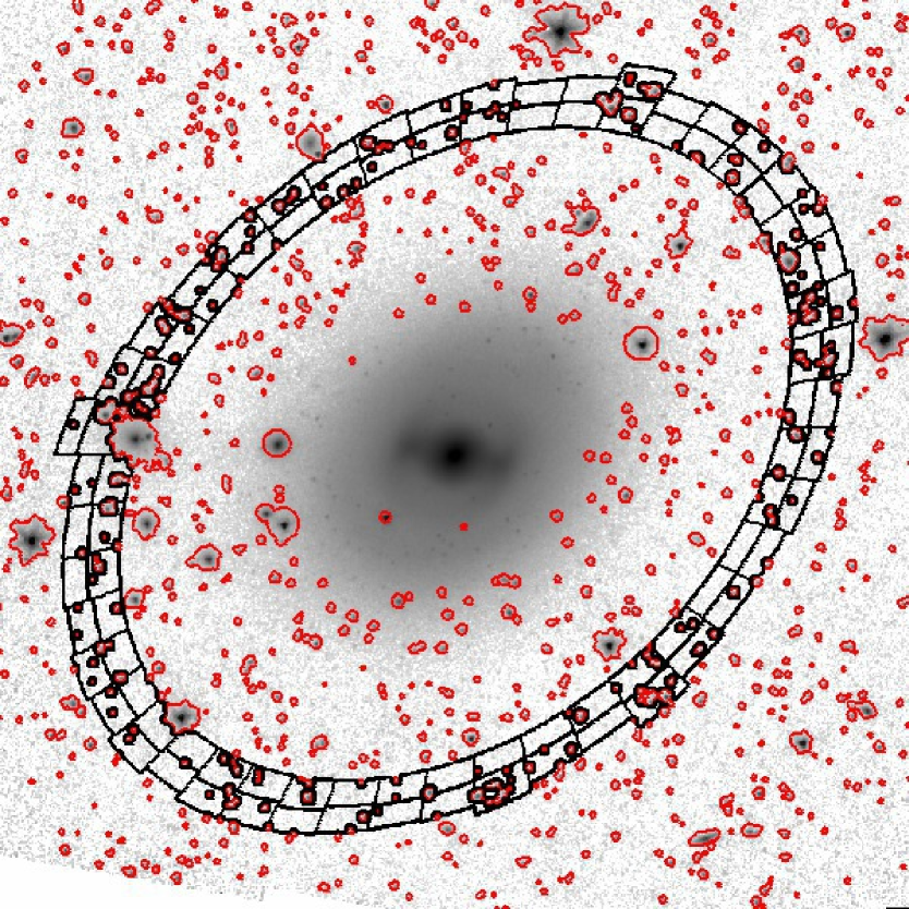
Figure 1.— Sample object mask (red) and sky boxes (black) overlaid on the 3.6 $\micron$ image of NGC0936. Note that the sky boxes are automatically grown in the radial direction to ensure that they all contain the same amount of unmasked pixels.

5. Pipeline 3: Surface photometry

In this section we describe in detail the inner workings of Pipeline 3. Briefly speaking, P3 first determines the background level of the images. It then locates the centroid of the galaxy and performs different sets of ellipse fits. Finally, it measures several properties such as asymptotic magnitudes, isophotal sizes and concentration indices.

5.1. Sky measurement

A careful determination of the background level and noise is essential to perform reliable surface photometry. This is often done by placing several “sky boxes” around each galaxy and measuring the corresponding background statistics in them. With large samples such as S⁴G it is desirable to implement this process in a way that is automatic yet flexible.

Pipeline 3 automatically places several sky boxes around each galaxy (see Fig. 1). This is done by defining two concentric and adjacent elliptical annuli that surround the entire galaxy. Each ring is then azimuthally subdivided into 45 sectors or boxes. Since these boxes will contain in general a certain amount of masked pixels, each box is grown radially outwards until each one contains 1000 unmasked pixels. We then measure the median sky level and local rms inside each box, as well as the large-scale rms between the sky levels of all boxes. While the number of 1000 pixels per box is to some extent arbitrary, it is chosen to provide a reliable measurement of the local rms, while at the same time yielding boxes that are small enough to be easily accommodated within our images. Note also that before using the P2 masks, we first grow the masked areas by 2 pixels to make sure that the faint wings of the PSF do not contaminate our sky measurements.

The sky boxes are initially placed by default at $2\times R_{25}$ from the galaxy center, but this value is modified as needed for each galaxy in order to ensure a proper background subtraction. To do this, we compare the values between the inner and outer rings to make sure that there are no significant differences, which could be a telltale sign of contamination from the galaxy itself. We double check this by verifying that the growth curve is flat (see Section 5.4). We also check that the boxes are not too close to the frame edges (which are noisier as a result of the dithering pattern), or that they do not fall in the adjacent frames (which may have a somewhat different background value). In cases with a complicated background structure, the pipeline allows one to manually distribute the sky boxes as deemed appropriate.

The distribution of measured background levels in the whole S⁴G sample is shown in Fig. 2. The histograms peak at $\mu\sim 24$ and $23.5$ AB mag arcsec^-2 for the 3.6 and 4.5 $\micron$ bands, respectively.

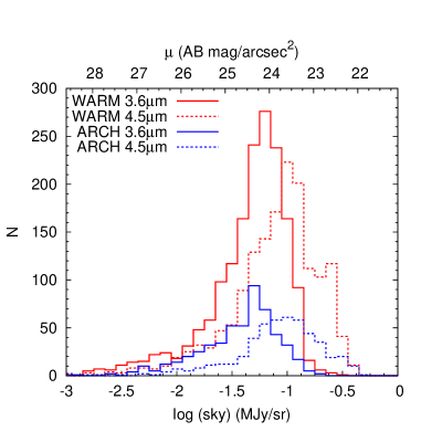
Figure 2.— Distribution of the sky level within the full S⁴G sample. Red and blue histograms show galaxies from the warm and archival (i.e. cryo) groups, respectively. Solid lines correspond to 3.6 $\micron$, and dashed ones to 4.5 $\micron$.

It is illustrative to verify whether our measured values of the background level agree with theoretical expectations. The background in the S⁴G images is almost entirely dominated by zodiacal light (or “zodi”) coming from dust grains in the ecliptic plane. Both the thermal emission of the grains and the scattered sunlight contribute to the zodi. At 3.6 and 4.5 $\micron$, both contributions are roughly equal. Thermal emission from interstellar cirrus in the Milky Way amounts to merely 1%-3% of the background in our images, as it peaks at much longer wavelengths (and the S⁴G sample specifically avoids the Galactic plane anyway). Contamination by the unresolved Cosmic Infrared Background is negligible at these bands compared to the zodi (Hauser et al. 1998).

Figure 3 shows how the observed sky level varies with the ecliptic latitude of each galaxy. As expected, since the primary source of background emission at these wavelengths is zodi, the distribution clearly peaks in the ecliptic plane. For each galaxy we retrieved from the FITS header the background level predicted for its Galactic coordinates and epoch of observation.^, The green curves in Fig. 3 are the upper and lower envelopes of these predicted values. We can see that both the dependency with ecliptic latitude and the range in background level at fixed latitude nicely agree with our measured values.

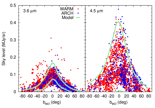
Figure 3.— Background level measured in our fully-reduced images as a function of the ecliptic latitude of each galaxy. Red and blue dots correspond to warm and archival galaxies. The green curves delimit the distribution of the zodi brightness predicted by the Spitzer background estimator.

Interestingly, about 30 WARM galaxies exhibit background levels at 3.6 $\micron$ well above the predicted values. A visual inspection of these images revealed a recurrent diffuse artifact, both in the main frame where the galaxy is and in the flanking one (Fig. 4). These few galaxies were observed in a narrow time window during August-September 2009, very shortly after the Spitzer’s warm phase began. This smooth background artifact may be therefore due to the detector temperature and bias not being settled yet at that time.

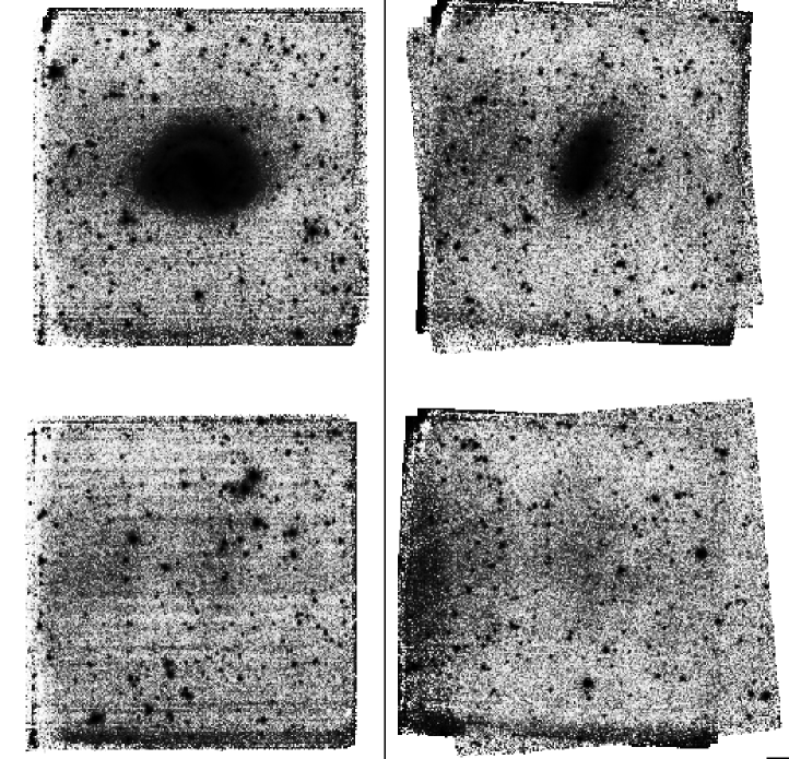
Figure 4.— Two sample images exhibiting a diffuse background artifact: NGC5597 (left) and UGC08507 (right). The smooth pattern is seen both in the main frame (top) and in the flanking one (bottom). A histogram equalization has been applied to exaggerate the brightness of this artifact. This structure only appears in $\sim 30$ of our galaxies.

Besides the background level itself, it is also important to characterize the background noise at different spatial scales, as this determines our ability to detect and measure faint structures at the outskirts of our galaxies. Figure 5 shows the distribution of the local, pixel-to-pixel noise in our images. The histogram for the warm galaxies is much narrower than that for the archival ones, which is expected given that the warm galaxies were imaged with the same observing strategy, whereas the archival come from a variety of different programs. In general we reach a local surface brightness sensitivity per pixel of $\sim 24$ and $\sim 26$ AB mag arcsec^-2 at $5\sigma$ and $1\sigma$, respectively.

Note, however, that these are values for individual pixels. When measuring the flux of a given extended source, this noise component scales down with the square root of the number of pixels in the region where the measurement is being performed. In particular, when measuring radial profiles at the outskirts of galaxies, this local noise component becomes negligible compared to the large scale background noise, which is given by the rms between the median sky values measured in the different boxes. As shown in Fig. 5, this large scale component peaks at 26-26.5 AB mag arcsec^-2 at a $5\sigma$ level, and $\sim 28$ AB mag arcsec^-2 at $1\sigma$. As a reference, $\mu_{3.6}=27$ AB mag arcsec^-2 corresponds to a stellar mass surface density of $1\,M_{\sun}\,\mathrm{pc}^{-2}$, adopting $M_{\star}/L_{3.6}=0.53$ as measured by Eskew et al. (2012); see also Meidt et al. (2014).

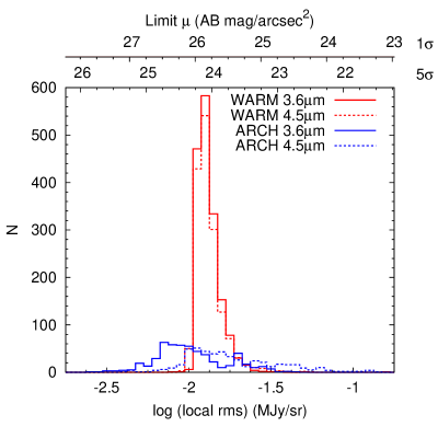
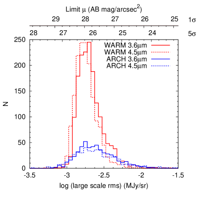
Figure 5.— Distribution of local, pixel-to-pixel noise (left) and large scale background noise (right) in the S⁴G images. WARM and ARCHIVAL galaxies are shown in red and blue, respectively. Solid and dashed lines correspond to 3.6 and 4.5 $\micron$. The corresponding surface brightness limit at $5\sigma$ and $1\sigma$ is shown at the top.

5.2. Radial profiles

Once the background level and noise have been measured, our pipeline proceeds to perform surface photometry on the images. We first use the IRAF task imcentroid to find accurate coordinates for the center of the galaxy. We then run the task ellipse (Jedrzejewski 1987; Busko 1996) to obtain radial profiles of surface brightness ($\mu$), ellipticity ($\epsilon$) and position angle (PA). We perform three separate runs of ellipse with different settings:

1. Fixed center; free $\epsilon$ and PA; radial resolution $\Delta r=6$″. We use these fits with a coarse radial increment to derive $\epsilon$ and PA in the outer parts of the galaxy, thus defining a global shape and orientation for each object. For each band, we provide values of $\epsilon$ and PA at two levels of surface brightness, $\mu=25.5$ and $26.5$ AB mag arcsec^-2. After testing how sensitive these values are to variations in the sky subtraction, input fitting parameters, amount of masked objects, etc., we recommend using the 25.5 values as they are more stable.

2. Fixed center; $\epsilon$ and PA fixed to the values at 25.5 AB mag arcsec^-2; $\Delta r=2$″. These fits have a finer radial resolution that matches the IRAC PSF at these wavelengths. By keeping $\epsilon$ and PA fixed and equal to the global outer values, these fixed-fits are ideal to measure disk scale-lengths, disk break radii, to perform 1D bulge-disk decompositions, etc. We also employ these profiles to measure the integrated magnitude of each galaxy from the growth curve (Sect. 5.4).

3. Fixed center; free $\epsilon$ and PA; $\Delta r=2$″. These free-fits with a fine resolution are well suited to study in detail the structural properties of features such as bars, which leave very characteristic signatures in the radial profiles of $\epsilon$ and PA. An example of these fits is shown in Fig. 6.

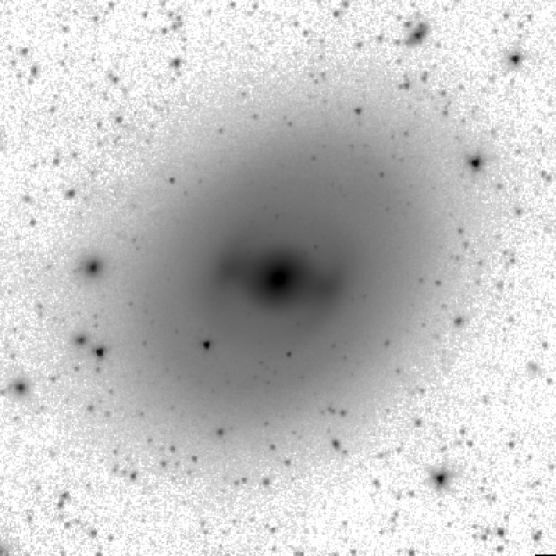
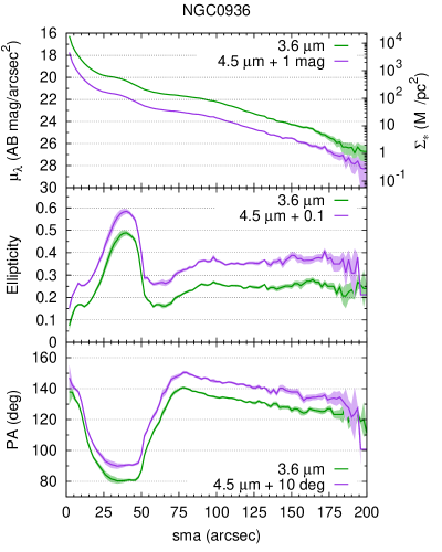
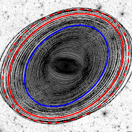
Figure 6.— Sample ellipse fit results for NGC0936 with free $\epsilon$ and PA, and a radial increment $\Delta r=2$″. The images to the left correspond to the 3.6 $\micron$ band. In the bottom one we have overlaid the ellipses fitted by our pipeline. The red solid ellipse corresponds to $\mu_{3.6}=25.5$ AB mag arcsec^-2, and the dashed one to $26.5$ AB mag arcsec^-2. The blue ellipse is the optical $D_{25}$ one from HyperLeda. In the radial profiles, offsets have been applied to the 4.5 $\micron$ data as indicated in the legend, to avoid overlapping. The right vertical scale in the top panel marks the stellar mass surface density for the 3.6 $\micron$ profile.

For simplicity and to improve the robustness of the fits, once we measure the central coordinates of galaxy, these are kept fixed during the ellipse fitting. However, the pipeline allows one to leave the center as a free parameter too. We have in fact performed such fits to study individual galaxies with offset bars (e.g. NGC3906, de Swardt et al. 2014, in prep.).

We normally begin the ellipse fitting at an intermediate radius, typically between $0.5-1\times R_{25}$, using the optical $\epsilon$ and PA from HyperLEDA as input guesses for the fitting routine. Starting at that initial radius, the ellipse fitting proceeds first outwards and then inwards.

It should be noted that the ellipse algorithm was specifically designed for galaxies with a smooth radial brightness distribution. It therefore works correctly for elliptical galaxies, but it does not cope well with features such as spiral arms or rings that can significantly modify the local luminosity gradient. As a result, ellipse can sometimes stop fitting at a given radius in spiral galaxies. Tuning the input parameters can sometimes fix this problem and provide a good fit, but in general this is a blind trial-and-error solution with an unpredictable outcome. Some authors have in fact circumvented this issue by automatically running ellipse tens or even hundreds of times on each image, varying the initial fitting parameters each time until a good fit is obtained (Jogee et al. 2004). While this approach can be practical in small images of distant galaxies, it is prohibitively time-consuming for the large images in S⁴G, where a single fit can take up to several minutes (and this is further complicated by the large number of galaxies in our sample). We thus decided to implement an optimized procedure that is better tailored to our needs. After each run of ellipse, the pipeline looks for any radial interval where the fit did not converge, and it then refits that particular radial interval alone. The process is then iterated several times to ensure that no radial gap is left unfit. In general most of our galaxies can be properly fit with a single ellipse run, but this automatic iterative process was of great help to handle troublesome cases that would have otherwise required considerable manual work.

In any case, for each galaxy we always visually inspect the output of the pipeline: we overlay the fitted ellipses on the galaxy image, and we plot the radial profiles of $\mu$, $\epsilon$ and PA, making sure that the results accurately probe the different structures within the galaxy.

Dwarf galaxies can be particularly challenging for our pipeline. They are often partially resolved into stars in our images, and their clumpy and patchy appearance can sometimes fool the ellipse fitting algorithm. For these galaxies we recommend not to overinterpret any signature in the $\epsilon$ and PA profiles without inspecting the images themselves. Since these galaxies normally lack well-defined large-scale structures such as bars, the profiles with fixed $\epsilon$ and PA are more suitable in these cases.

We have released all these ellipse fits in the form of ASCII tables containing the full output of the ellipse task. These tables not only include radial profiles of $\mu$, $\epsilon$ and PA, but also other quantities such as the harmonic deviations from a perfect ellipse, which are commonly used to quantify the boxiness/diskiness of the isophotes at different radii (e.g. Carter 1978; Kormendy & Bender 1996).

Apart from the usual output from ellipse, we also include in our ASCII profiles additional columns that are specific to the IRAC data used here. In particular, the IRAC photometry needs to be corrected for the extended wings of the PSF and the diffuse light that is scattered throughout the detector. Here we rely on the extended source aperture correction provided in the IRAC Instrument Handbook. Given an elliptical aperture with major and minor radii $a$ and $b$, if $F_{\mathrm{obs}}$ is the total observed flux inside such an aperture, the corrected flux is given by:

$$F_{\mathrm{corr}}(r_{\mathrm{eq}})=F_{\mathrm{obs}}(r_{\mathrm{eq}})\times(Ae^{-r_{\mathrm{eq}}^{B}}+C)$$ (1)

In this expression $r_{\mathrm{eq}}=\sqrt{ab}$ is the equivalent radius of the elliptical aperture, in arcseconds. The coefficients $A$, $B$ and $C$ are equal to 0.82, 0.370 and 0.910, respectively, at 3.6 $\micron$, and 1.16, 0.433 and 0.94 at 4.5 $\micron$.

Similarly, if $I_{\mathrm{obs}}$ is the surface brightness along an isophote (rather than the total flux inside that radius as before), the aperture-corrected surface brightness can be obtained by performing a series expansion on the previous equation:

$$I_{\mathrm{corr}}(r_{\mathrm{eq}})= I_{\mathrm{obs}}(r_{\mathrm{eq}})\times(Ae^{-r_{\mathrm{eq}}^{B}}+C)-$$

$$-ABr_{\mathrm{eq}}^{B-2}e^{-r_{\mathrm{eq}}^{B}}F_{\mathrm{obs}}(r_{\mathrm{eq}})/(2\pi)$$ (2)

Our ASCII tables include radial profiles with and without these aperture corrections. These corrections are estimated to be uncertain at a 5%-10% level. We have always applied the extended source aperture correction at all radii in our profiles. However, the reader should keep in mind that the point source corrections might be more suitable at very small radii ($r\lesssim 8$-$9$″), especially if the nucleus is bright and compact.

Finally, all the released profiles have been corrected for foreground extinction, using the color excess map of Schlegel et al. (1998) and the Milky Way extinction curve of Li & Draine (2001). Nevertheless, at 3.6 and 4.5$\micron$ this extinction correction is typically around 0.005 mag.

5.3. Error analysis

The pipeline also estimates the uncertainty in $\mu$, $\epsilon$ and PA at different radii. For $\epsilon$ and PA we rely on the errors determined by the ellipse task, which result from the internal errors in the harmonic fit (Busko 1996). As for $\mu$, the error provided by ellipse is derived from the rms of the pixel values along each isophote, so it mostly reflects azimuthal variations of the stellar emission at a given radius rather than the true uncertainty of the mean surface brightness at that radius. We therefore opted to measure the error in $\mu$ ourselves.

If $I$ is the incident pixel intensity, prior to sky subtraction, and $I_{\mathrm{sky}}$ is the sky level, then the surface brightness is given by:

$$\mu=-2.5\log(I-I_{\mathrm{sky}})+K$$ (3)

where $K$ includes the magnitude zero-point plus any other global multiplying factor, such as the aperture corrections mentioned before. Following the methodology detailed in Gil de Paz & Madore (2005) and Muñoz-Mateos et al. (2009a), the uncertainty in $\mu$ can be estimated as:

$$\Delta\mu=\sqrt{(\Delta K)^{2}+\left(\frac{2.5\log(e)}{I-I_{\mathrm{sky}}}\right)^{2}(\Delta I^{2}+\Delta I^{2}_{\mathrm{sky}})}$$ (4)

The error in $K$ is dominated by the uncertainty in the aperture corrections, and is of the order of 5-10% as explained in the previous section. Since any change in $K$ will merely translate into a global offset of the radial profiles, the values of $\Delta\mu$ in our ASCII tables and plots do not explicitly include the contribution of $\Delta K$.

We computed $\Delta I$, which is the error in the incident pixel intensity, by assuming poissonian statistics:

$$\Delta I=\sqrt{\frac{I}{g_{\mathrm{eff}}N_{\mathrm{isophote}}}}$$ (5)

where $g_{\mathrm{eff}}$ is the effective gain and $N_{\mathrm{isophote}}$ is the number of pixels within each isophote. The effective gain, in turn, was derived from the nominal detector gain and the exposure time of each pixel according to the weight maps.

The term $\Delta I_{\mathrm{sky}}$ represents the uncertainty in the background level, and was obtained as:

$$\Delta I_{\mathrm{sky}}=\sqrt{\frac{\sigma_{\mathrm{local}}^{2}}{N_{\mathrm{isophote}}}+\max\left(\sigma^{2}_{\mathrm{large}}-\frac{\sigma_{\mathrm{local}}^{2}}{N_{\mathrm{box}}},0\right)}$$ (6)

where $\sigma_{\mathrm{local}}$ and $\sigma_{\mathrm{large}}$ are the local and large scale background rms, respectively, as described in Section 5.1. Here $N_{\mathrm{isophote}}$ is, again, the number of pixels along a given isophote, and $N_{\mathrm{box}}$ is the number of pixels inside the boxes used to measure the background level.

The first term in Eq. 6 reflects the contribution of the local, pixel-to-pixel noise to the final error in the surface brightness. This contribution scales down as $1/\sqrt{N_{\mathrm{isophote}}}$, so it becomes negligible at large radii, where the flux is averaged over a large number of pixels. It is the second term, the large-scale noise, the one that dominates the error budget at large radii. Note that the measured rms between the sky values in the different boxes is partly contaminated by the local noise, in the sense that even if there were no true large-scale fluctuations, the rms between the sky boxes would be $\sigma_{\mathrm{local}}/\sqrt{N_{\mathrm{box}}}$, on average. The correction term in Eq. 6 accounts for this.

5.4. Asymptotic magnitudes

From the surface photometry we measure the asymptotic magnitude of each galaxy by extrapolating the growth curve to infinity. To do this we use the profiles with fixed $\epsilon$ and PA and 2″ resolution. As an example, the bottom panel of Figure 7 shows the 3.6 $\micron$ growth curve of NGC0936, which rises fast at the center and then slowly approaches a flat regime. To determine this asymptotic value, we first compute the gradient of the growth curve at all radii. In the outer parts of the galaxy, the gradient at a given radius and the magnitude inside that radius follow a linear trend (top panel). We then apply a linear fit whose y-intercept (the magnitude for a flat gradient) is by definition the asymptotic magnitude.

Note that growth curves are often used in shallow images to recover the flux buried beneath the noise in the outskirts of galaxies. This is not the case in the S⁴G images, which are deep enough to always comfortably reach the flat regime of the growth curve. Therefore, in practice there is no extrapolation involved when fitting the growth curves of our galaxies. In this regard, the error bugdet in the surface photometry is dominated by the large-scale rms, and not by any possible non-zero slope in the growth curve.

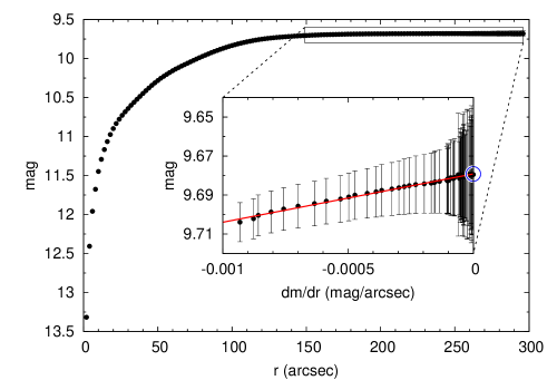
Figure 7.— Illustration of how the asymptotic magnitudes are computed. The main panel shows the 3.6 $\micron$ growth curve of NGC0936, that is, the integrated magnitude as a function of radius. The small inset shows the magnitude as a function of the magnitude gradient for the data-points in the flat portion of the growth curve. The red line represents a linear fit to both quantities. The asymptotic magnitude is the y-intercept of this fit, namely, the magnitude for a flat gradient (blue circle).

Once we have determined the asymptotic apparent magnitudes, we derive the absolute ones using redshift-independent distances from NED whenever available (79% of the sample), and redshift-dependent ones otherwise, assuming $H_{0}=71$ km s^-1 Mpc^-1. For those galaxies with more than one redshift-independent distance measurement (61% of the whole sample), the typical rms between the different measured distances is $\sim 15$%, which translates into an error of $\sim 0.3$ mag in the absolute magnitude. While this is not strictly speaking a true formal uncertainty, for such nearby galaxies it provides a more realistic estimate of the actual distance error than the uncertainty in the radial velocity, which is just $\sim 0.3$% for our galaxies.

In Fig. 8 we plot the 3.6$\micron$ absolute magnitude for all our galaxies as a function of their optical morphological type as given by HyperLEDA (the 4.5$\micron$ values follow a very similar trend). The conversion to stellar mass in the rightmost vertical axis was done via the $M_{\star}/L$ value of Eskew et al. (2012). At the late-type end of the sequence, the stellar mass rises monotonically from $\sim 5\times 10^{8}$ $M_{\sun}$ for irregular galaxies to $1-2\times 10^{10}$ $M_{\sun}$ for Sc ones. The trend then remains remarkably flat out to S0 galaxies, beyond which the stellar mass increases again for elliptical galaxies. The rms in stellar mass for each bin of Hubble type is typically between 0.5-0.6 dex, or a factor of 3-4.

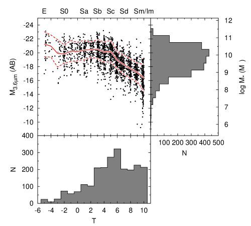
Figure 8.— Stellar mass and absolute magnitude at 3.6$\micron$ of all S⁴G galaxies as a function of their morphological type, together with the corresponding histograms of both quantities. The solid and dashed lines show the median trend and rms in bins of $\Delta T=1$.

5.5. Concentration indices

Central light concentration is one of the parameters that varies most prominently along the Hubble sequence, and was in fact used early to modify Hubble’s original classification scheme (Morgan 1958). Light concentration and other non-parametric estimators such as the asymmetry, clumpiness, second-order moment or Gini coefficient, have been extensively used over the years to quantify the morphology of nearby and distant galaxies (Bershady et al. 2000; Conselice 2003; Conselice et al. 2003; Abraham et al. 1996b, a, 2003; Lotz et al. 2004; Taylor-Mager et al. 2007; Muñoz-Mateos et al. 2009a; Holwerda et al. 2011). In particular, Holwerda et al. (2013) presented a detailed study of the quantitative morphology of the S⁴G galaxies through a suite of commonly used non-parametric estimators.

Here we present the concentration indices derived from the growth curves measured by our pipeline. Among the different definitions existing in the literature, we settled on $C_{31}$ (de Vaucouleurs 1977) and $C_{82}$ (Kent 1985), defined as follows:

$$C_{31} = \frac{r_{75}}{r_{25}}$$ (7)

$$C_{82} = 5\log\left(\frac{r_{80}}{r_{20}}\right)$$ (8)

where $r_{x}$ is the semi-major axis of the ellipse enclosing $x$% of the total luminosity of the galaxy. There is some discrepancy in the literature regarding how the total luminosity is measured when computing concentration indices; here we simply use the asymptotic magnitudes described before. Also, unlike concentration indices derived from Sérsic fitting, our values are truly non-parametric, in the sense that we do not assume any functional form for the radial profiles or the growth curves.

For each galaxy and band we computed both concentration indices. The results are presented in Sec. 6.1, where we investigate why galaxies with the same stellar mass can exhibit vastly different morphologies and concentration indices.

5.6. Galaxy sizes and shapes

From the growth curves we have also obtained effective radii ($r_{\mathrm{eff}}$) containing half of the total asymptotic luminosity, independently at both IRAC bands. Radial gradients in age, metallicity and internal extinction have a negligible impact at these wavelengths; therefore, our half-light radii can be safely interpreted as half-mass radii. Given that we measured $r_{\mathrm{eff}}$ along the major axis of elliptical isophotes, our values do not need to be corrected for inclination, as is the case in studies employing circular apertures. Also, since we do not perform any sort of Sérsic or similar fitting, the values that we provide constitute the true effective radius of each galaxy, and not the effective radius of a simple model fitted to that galaxy. In Sect. 6.2 we discuss in detail the stellar mass-size relation of the S⁴G galaxies for different morphologies.

The effective radii depend on the level of central concentration, in the sense that highly-concentrated galaxies tend to have small values of $r_{\mathrm{eff}}$ compared to the overall extent of those galaxies. Therefore, it is also desirable to measure the global sizes and shapes of our galaxies, including their outermost parts. Here we follow an RC3-like approach and measure the radius, ellipticity and position angle at 25.5 and 26.5 AB mag arcsec^-2, both at 3.6 and 4.5$\micron$ (that is, four sets of measurements for each galaxy). We recommend using the 25.5 values at 3.6$\micron$ to characterize the overall extent of the S⁴G galaxies. Even though there is always plenty of detectable emission beyond that surface brightness level, ellipse fitting becomes less reliable and more sensitive to convergence issues, object masking and background subtraction. The distribution of isophotal sizes as a function of stellar mass and morphology is presented in Sect. 6.2.

Regarding the outer isophotal ellipticities, they can be used as a photometric proxy for the disk inclination in the case of spiral galaxies. We have in fact used the P3 ellipticities to deproject our galaxies and recover the intrinsic shapes of rings and bars, for instance (Comerón et al. 2013; Muñoz-Mateos et al. 2013).

Note, however, that this is complicated by the fact that (a) disks may not be perfectly circular when viewed face-on, and (b) the intrinsic vertical thickness of disks and bulges/haloes will distort the outermost isophotes at high inclinations (see, e.g., Ryden 2004, 2006 and references therein for a discussion on both issues). The influence of the vertical thickness is particularly obvious in our deep IRAC images, given that thick disks and spheroids are primarily composed of old stellar populations, which show up prominently at these wavelengths. Users should therefore keep this in mind when studying highly-inclined galaxies in our sample (Comerón et al. 2011). We will present inclinations derived from multicomponent 2D fitting of the galaxy images in a forthcoming paper (Salo et al. 2014, in prep.).

6. Results and discussion

6.1. Variations in concentration and morphology at fixed stellar mass

Figure 9 shows the distribution of the $C_{82}$ index at 3.6$\micron$ as a function of the stellar mass for all S⁴G galaxies. Figure 10 displays the same information in histogram form. None of these plots change noticeably when using $C_{31}$ and/or the 4.5$\micron$ data instead.

The concentration index distribution exhibits a pronounced narrow peak centered at $C_{82}\sim 2.8$-$3$, and a much broader one peaking at $C_{82}\sim 4.5$-$5$. The first group corresponds to disk-dominated galaxies; indeed, the theoretical concentration index for a perfectly exponential profile is 2.8. The second group comprises bulge-dominated galaxies and ellipticals. The “L”-shaped distribution of concentration vs. stellar mass shown in Fig. 9 nicely describes how the spatial distribution of old stars within galaxies varies across the Hubble sequence. For galaxies later than Sc, the concentration index remains roughly constant at the value expected for disk-dominated galaxies, with some scatter but no obvious dependence on the stellar mass. But for galaxies earlier than Sc the situation changes, and now the concentration index ranges anywhere from a disk-dominated profile to a highly concentrated one. A similar distribution was found by Scodeggio et al. (2002) in their analysis of the $H$-band photometry of galaxies in nearby clusters. They found that galaxies with $L_{H}<10^{10}L_{\sun}$ exhibit a small and constant concentration index, as well as blue optical-IR colors. At $L_{H}>10^{10}L_{\sun}$ galaxies were found to span a large range of concentration indices, with redder colors.

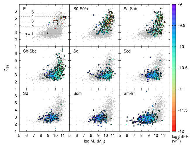
Figure 9.— Concentration index $C_{82}$ at 3.6$\micron$ as a function of total stellar mass. The gray datapoints show the full S⁴G sample, whereas the colored ones correspond to galaxies with different Hubble types, as indicated in each panel. The color indicates the extinction-corrected specific SFR, computed from GALEX and Spitzer data as explained in the text. As a reference, in the top-left panel we plot with dashed horizontal lines the theoretical concentration indices for Sérsic profiles with different indices $n$.

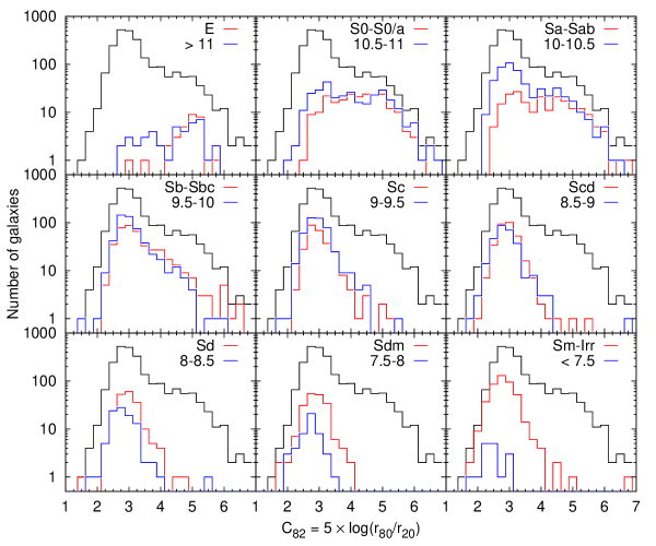
Figure 10.— Histograms of the concentration index $C_{82}$ at 3.6$\micron$ for the S⁴G galaxies. The black histogram is the same in all panels, and corresponds to the full sample. The red and blue histograms show galaxies grouped in bins of morphological type and $\log M_{*}$, respectively.

To better quantify the structural variety of the S⁴G galaxies, in Fig. 11 we show the median profiles after grouping the galaxies in bins of stellar mass and concentration. Based on the fact that $C_{82}=2.8$ for a pure exponential profile and $C_{82}=5.3$ for a de Vaucouleurs one, we use these values to define four bins of mass concentration, as shown in Fig. 11: blue and green curves are the median profiles of disk-dominated galaxies, with the blue ones being less concentrated than the green ones. On the other hand, orange and red curves correspond to bulge-dominated galaxies, with the latter being the most concentrated ones.

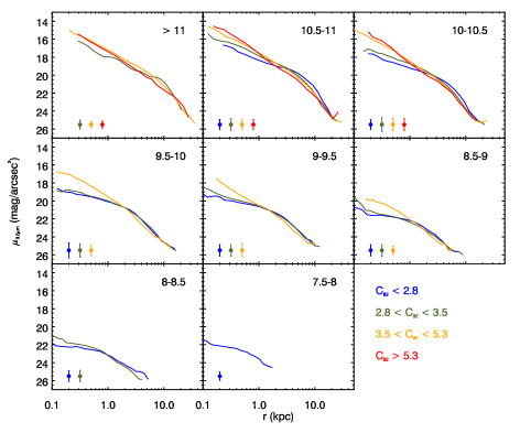
Figure 11.— Median surface brightness profiles of the S⁴G galaxies in bins of $\log M_{\sun}$, as indicated by the numbers at the top-right of each panel, and concentration index $C_{82}$, according to the color scheme in the legend. Prior to computing the median, the profiles were corrected for inclination and resampled to a commom physical scale in kpc. At least five galaxies were required in each bin to derive the median. The errorbars in each panel show the $\pm 1\sigma$ deviation around the median profile in each case.

In galaxies more massive than $10^{10}\,M_{\sun}$, the observed differences in concentration at a fixed mass are driven by variations in the global radial stellar structure over scales of many kpc, all the way from the center of the galaxies to their outer parts. However, for galaxies less massive than $10^{10}\,M_{\sun}$ the situation is different: differences in concentration between the blue and green curves (both disk-dominated) are mostly due to the presence or absence of central bright features smaller than 1 kpc; the disks at $r>1\,\mathrm{kpc}$ are otherwise very similar in terms of surface density and slope.

In the following two subsections we investigate in more detail why galaxies with the same stellar mass and morphological type present such varied radial structure and concentration indices.

6.1.1 Spread in concentration above $10^{10}\,M_{\sun}$

According to Fig. 9, the structural transition between low- and high-concentration galaxies occurs at stellar masses between $10^{10}$ and $10^{11}\,M_{\sun}$. Previous studies based on optical imaging and spectroscopy have found abrupt transitions in the stellar ages and star formation histories in the same mass interval (Kauffmann et al. 2003; Brinchmann et al. 2004), with stellar populations suddenly becoming older when going from low-mass, disk-dominated galaxies to more massive, highly-concentrated ones.

To quantify changes in the stellar populations of the S⁴G galaxies we made use of GALEX measurements in the far and near ultraviolet. Bouquin et al. (2015, submitted) measured FUV and NUV surface photometry and asymptotic magnitudes for the S⁴G galaxies following the same methodology described here for the Spitzer images. Here we use their measurements to derive extinction-corrected star formation rates (SFR).

For each galaxy we first estimated the internal dust extinction via the integrated FUV$-$NUV color, following the prescription calibrated by Muñoz-Mateos et al. (2009b) on nearby galaxies. While this recipe is a good proxy for internal extinction in normal star-forming spirals, it overestimates the true extinction in elliptical galaxies, where a significant fraction of the observed UV reddening is due to the intrinsicially old and red stellar populations. It also overestimates the extinction in Sdm-Irr galaxies, which tend to have somewhat redder UV colors than other low-mass disks with similar dust content, possibly due to differences in the extinction law, dust geometry, or a bursty star formation activity. Therefore, we only relied on the FUV$-$NUV color to determine the internal extinction in the disk-dominated galaxies of our sample. Following Muñoz-Mateos et al. (2009b), for elliptical galaxies we adopted a constant extinction in the FUV of 2 mags, and 0.5 mags in the case of Sdm-Irr galaxies. The extinction-corrected FUV luminosities were then converted into SFR via the calibration of Kennicutt (1998). Note that in elliptical galaxies most of the UV light is not associated to recent star formation, so their true SFR is lower than the value resulting from the Kennicutt (1998) prescription.

The data-points in Fig. 9 are colored according to their specific SFR (sSFR, the SFR per unit of stellar mass). The transition from low- to high-concentration galaxies in the mass regime between $10^{10}$ and $10^{11}\,M_{\sun}$ is accompanied by a decrease of one order of magnitude in the sSFR, which drops from $\sim 10^{-10.5}\,\mathrm{yr}^{-1}$ in massive, low-concentration galaxies to $\sim 10^{-11.5}\,\mathrm{yr}^{-1}$ in high-concentration galaxies with the same stellar mass. The same decrease in sSFR is found in spectroscopic studies, where the sSFR is estimated from spectral measurements such as the break at 4000Å or the H$\alpha$ equivalent width (Kauffmann et al. 2003; Brinchmann et al. 2004).

This drop in sSFR with increasing concentration does not occur all at once for all morphological types, though. Figure 9 demonstrates that it is only in S0/a galaxies and earlier types that the sSFR drops below $\sim 10^{-11}\,\mathrm{yr}^{-1}$ in highly-concentrated objects. In these galaxies the high-concentration and red colors result from the dominant contribution of large bulges and stellar haloes to the total light. But in the morphological range between Sa and Sbc, highly-concentrated galaxies still exhibit a relatively high sSFR of $\sim 10^{-10}\,\mathrm{yr}^{-1}$, similar to the sSFR of less concentrated galaxies in the same morphological regime.

What is the physical nature of these galaxies with a concentrated stellar mass distribution but high sSFR? A visual inspection of these objects reveals that they are a mixed bag of galaxies with very different physical properties, which can be nevertheless sorted out into three broad categories (Fig. 12):

1. Barred galaxies with prominent nuclear rings, such as NGC 7552, NGC 4593 or NGC 1365. The strong bars in these galaxies drive gas inwards, but this gas eventually stalls in a nuclear ring, most likely associated with the Inner Lindblad Resonance (Regan et al. 1999; Sheth et al. 2000, 2005). This shrinks $r_{20}$, the radius of the isophote containing 20% of the total luminosity of the galaxy, thus increasing the concentration index $C_{82}$ in these galaxies. Note that given the intense star formation activity in nuclear rings and their elevated gas and dust content, non-stellar sources can locally dominate the 3.6 and 4.5 $\micron$ emission in these rings. Nevertheless, the clean stellar mass maps resulting from our Pipeline 5 (Meidt et al. 2012; Querejeta et al. 2014) still reveal a prominent central concentration of stellar mass in these galaxies, indicating that bar-driven gas inflows play a key role in the secular assembly of (pseudo-)bulges (Kormendy & Kennicutt 2004; Sheth et al. 2005).

2. Interacting systems such as NGC 2782, NGC 7714 or NGC 5534. These galaxies often exhibit up-bending radial profiles, with a steep inner disk followed by a flatter outer one, normally accompanied by tidal features in the outermost regions. This decreases $r_{20}$ and increases $r_{80}$, yielding high concentration indices. Numerical simulations of minor mergers such as those by Younger et al. (2007) can reproduce this radial structure: the interaction leads to gas inflows that contract the inner radial profile, while at the same time the outwards transfer of angular momentum expands the outer disk. Also, the sSFR is temporarily enhanced in these galaxies during the interaction, with prominent star forming knots that are clearly visible in the GALEX images.

3. Galaxies with compact bulges and smooth extended disks, often undisturbed as in NGC 3642. This again leads to a small $r_{20}$ and large $r_{80}$. While these extended outer disks often have low surface brightness in the infrared, they can be much brighter at UV wavelengths, as happens with NGC 3642. These so-called extended UV disks are typically found in $\sim$ 10% - 20% of nearby galaxies (Gil de Paz et al. 2005; Thilker et al. 2005, 2007), but the origin of these galaxy-wide star formation events is still under debate.

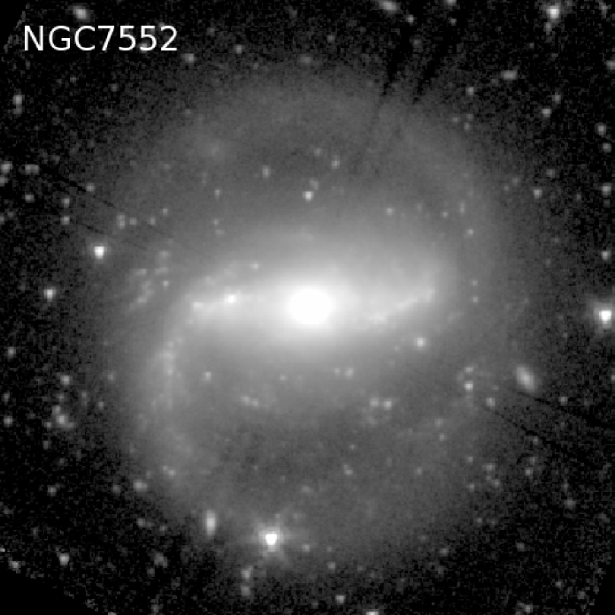
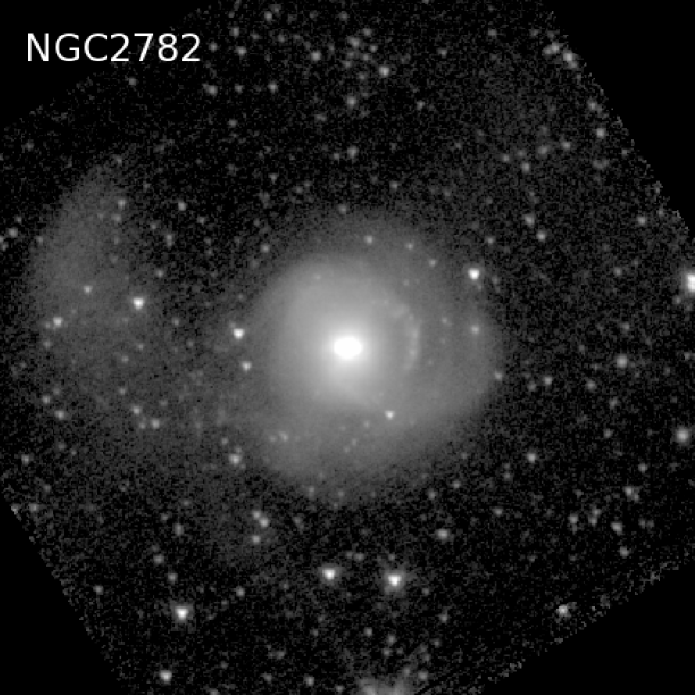
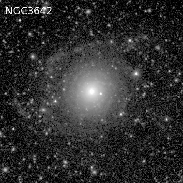
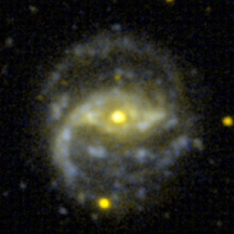
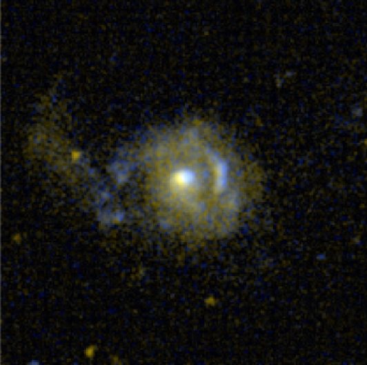
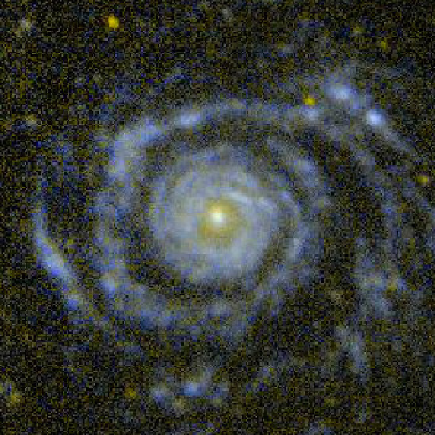
Figure 12.— Three sample S⁴G galaxies with high concentration indices at 3.6 $\micron$ ($C_{82}\sim 5.0-5.5$) and also high specific SFR ($\lesssim 10^{-10}\,\mathrm{yr}^{-1}$): NGC 7552, a barred spiral, NGC 2782, an interacting disk, and NGC 3642, a galaxy with a compact nucleus/bulge and a diffuse extended disk. The top panels show the S⁴G images at 3.6 $\micron$, whereas the bottom panels display false color FUV$+$NUV images from GALEX (Gil de Paz et al. 2007).

In brief, for stellar masses above $10^{10}\,M_{\sun}$, galaxies with a centrally concentrated radial distribution of old stars are either (a): quiescent galaxies with a prominent stellar bulge/halo, or (b) star-forming galaxies with central mass concentrations due to a variety of mechanisms such as bar- or merger-driven inflows.

6.1.2 Spread in concentration below $10^{10}\,M_{\sun}$

Figure 9 shows that galaxies with stellar masses below $10^{10}\,M_{\sun}$ still exhibit a considerable scatter in the concentration index at any given mass. While all these galaxies have concentration indices broadly consistent with a disk-dominated profile, the actual values can range anywhere from $C_{82}\sim 2$ to $\sim 3.5$. Moreover, this scatter in $C_{82}$ does not seem to be correlated with changes in the sSFR, as was the case in the more massive galaxies analyzed before.

To ascertain the origin of these structural variations in low mass disks, we visually inspected galaxies with the same stellar mass but extreme values of concentration. Figure 13 displays several representative examples.

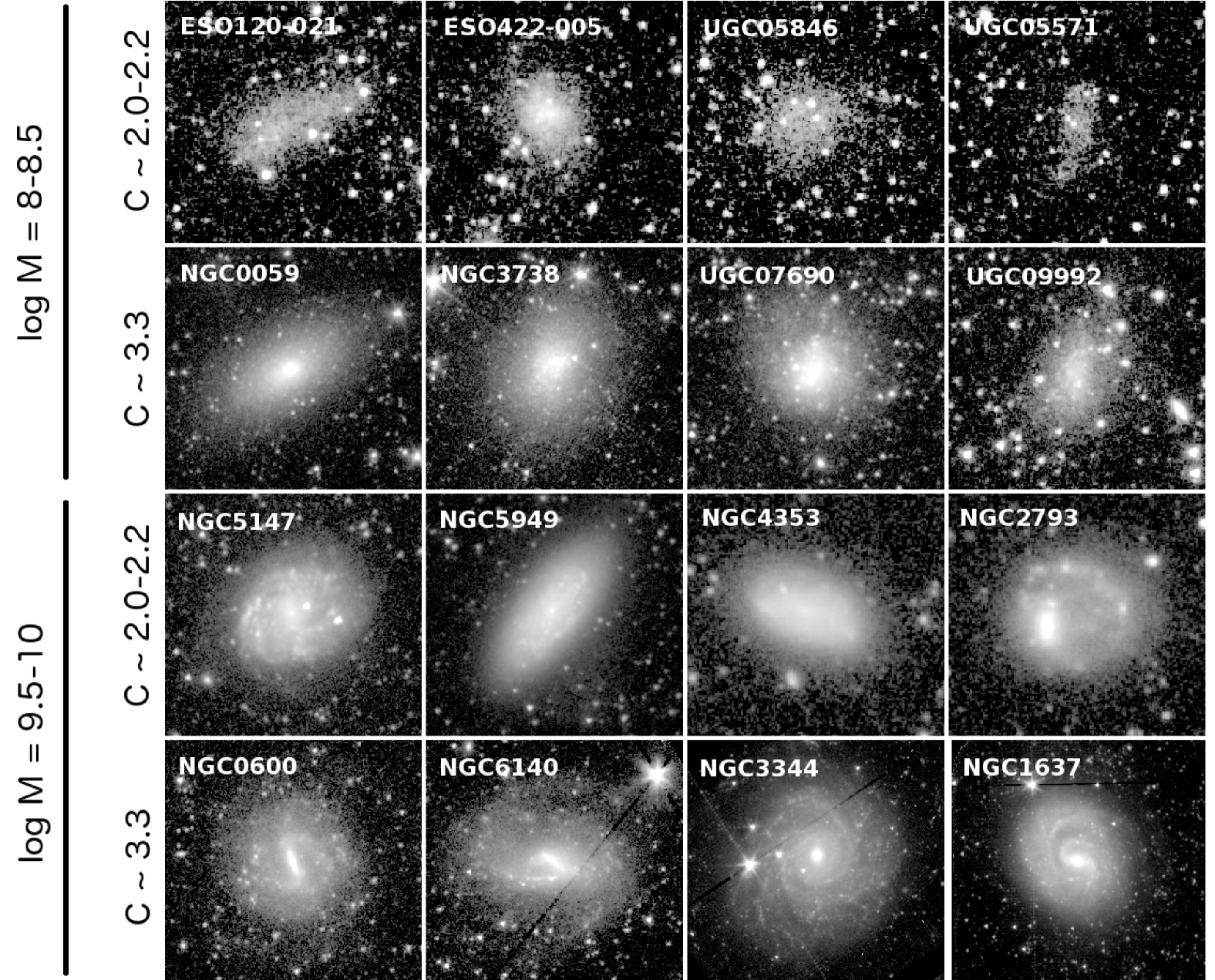
Figure 13.— First row: galaxies with stellar masses between $10^{8}-10^{8.5}\,\mathrm{M_{\sun}}$ and low concentration indices ($C_{82}\sim 2.0-2.2$). Second row: galaxies with the same stellar mass as those in the first row, but higher concentration values ($C_{82}\sim 3.3$). Third row: more massive disks with masses around $10^{9.5}-10^{10}\,\mathrm{M_{\sun}}$, but low concentration. Fourth row: same stellar mass as in the third row, but higher concentration.

The top two rows show very low-mass dwarf disks, all of them with stellar masses between $10^{8}-10^{8.5}\,\mathrm{M_{\sun}}$. The objects in the first row are characterized by very low concentration indices of $C_{82}\sim 2.0-2.2$ (smaller than for an exponential profile), whereas those in the second row all have $C_{82}\sim 3.3$ (larger than for an exponential). This higher concentration is due to central aggregations of stars (usually resolved in our images) that are absent in the first group of galaxies. GALEX images of some of these concentrated dwarfs, like NGC 0059 and NGC 3738, reveal bluer UV colors in the central parts than in the outskirts, possibly hinting to an outside-in formation for these objects.

The third and fourth rows in Fig. 13 correspond to more massive disks, with stellar masses between $10^{9.5}-10^{10}\,M_{\sun}$. Galaxies in the third row present $C_{82}\sim 2.0-2.2$, while those in the fourth row have $C_{82}\sim 3.3$. In this case the higher concentration results from bright bars as in NGC 0600 or NGC 6140. Unbarred galaxies can be also concentrated if they host bright and compact (pseudo-)bulges, as in NGC 3344. In contrast, low concentrated disks in this mass range either have weakly-defined bars (NGC 5147) or no bars at all (NGC 5949). Moreover, some galaxies such as NGC 4353 have bright inner disks that lead to central plateaus in their radial profiles, leading to concentration indices lower than those expected for an exponential profile.

We also find a wealth of asymmetric galaxies which may have recently undergone gravitational interactions. In some of them, like NGC 2793, the stellar mass is so dislodged that the radial surface density is almost flat, leading to very low concentration indices. On the other hand, galaxies like NGC 1637 exhibit a much milder asymmetry, and therefore have higher concentration values (Zaritsky et al. 2013 and references therein).

In summary, even though galaxies with stellar masses below $10^{10}\,M_{\sun}$ tend to have low concentration, at any given mass variations in concentration are still present, due to the presence of central star clusters, bars, pseudo-bulges, or lack thereof.

6.2. The stellar mass-size relation

The mass-size relation provides very stringent constraints on models of galaxy formation and evolution. From a cosmological point of view, the trend between increasing galaxy size and mass reflects, to first order, the physical connection between the mass of the dark matter halo and its angular momentum. Indeed, in a $\Lambda$CDM cosmology the characteristic size of a disk should scale as $M^{1/3}_{\mathrm{halo}}$ (Fall & Efstathiou 1980; Mo et al. 1998). In practice, though, the stellar mass-size relation also depends on whether the halo gas conserves its angular momentum as it settles onto the disk, how efficiently that gas is later converted into stars, the impact of AGN and stellar feedback, and whether internal and external processes rearrange stars within the galaxy.

The mass-size (or luminosity-size) relation has been extensively explored both in the local universe (see, e.g., Kauffmann et al. 2003; Shen et al. 2003; Courteau et al. 2007; Fernández Lorenzo et al. 2013; Lange et al. 2014) and at high redshift (e.g. Barden et al. 2005; Trujillo et al. 2004, 2006; Franx et al. 2008; van der Wel et al. 2014). Here we take advantage of the little sensitivity of the IRAC bands to dust extinction and $M/L$ variations to derive a self-consistent stellar mass-size relation in the local universe.

In Fig. 14 we plot $R_{25.5}$, the semi-major radius at $\mu_{3.6}=25.5$ AB mag arcsec^-2, as a function of the total stellar mass for all S⁴G galaxies. We find an obvious and expected monotonic trend, in the sense that galaxies with higher stellar mass are also larger. However, the slope of this trend is not constant, as galaxies of different Hubble types populate different areas in this plot, defining clearly distinct sequences. As in Figs. 8 and 9, Sc galaxies constitute a well-defined transition type in this diagram, in the sense that earlier-type galaxies are up to a factor of $\sim 10$ more massive than later-type ones for the same outermost size $R_{25.5}$.

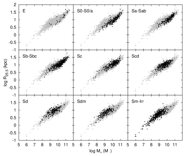
Figure 14.— Semi-major radius at $\mu_{3.6}=25.5$ AB mag arcsec^-2 as a function of stellar mass of all S⁴G galaxies (gray dots), grouped by their morphological type (black dots).

Isophotal radii represent a robust metric of global galaxy sizes in the nearby universe, but their applicability to distant galaxies is hampered by cosmological surface brightness dimming. In order to facilitate the comparison of the S⁴G mass-size relation with observations at higher redshits, we have also measured the effective radius $r_{\mathrm{eff}}$ of our galaxies. In Fig. 15 we show the trend between the effective radius at 3.6 $\micron$ and the total stellar mass of our galaxies, in bins of morphological type. As explained in Sect. 5.6, $r_{\mathrm{eff}}$ was measured along the semi-major axis of elliptical apertures, so no inclination corrections are required. The diagonal lines in this plot represent different values of the average stellar mass surface density inside $r_{\mathrm{eff}}$, that is, $0.5M_{\star}/(\pi r_{\mathrm{eff}}^{2})$. Points are again color-coded according to their extinction-corrected sSFR.

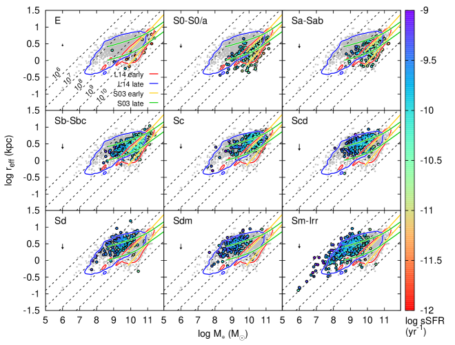
Figure 15.— Effective radius along the semi-major axis at 3.6 $\micron$ as a function of the total stellar mass, grouped by morphological type. Data-points are color-coded based on the sSFR of each galaxy (see Sect. 6.1.1 for details). The dashed diagonal lines mark constant values of the average stellar mass surface density inside $r_{\mathrm{eff}}$. The red and blue contours delineate the mass-size relation of early- and late-type galaxies found by Lange et al. (2014) in the GAMA survey. The orange and green curves correspond to the early- and late-type distributions found by Shen et al. (2003) on SDSS data. The latter were derived from circular apertures; the vertical arrows in each panel show how our ellipse-based measurements would shift downwards had we used circular apertures, given the median ellipticity in each bin of morphological type.

The main difference with respect to the mass-size relation based on isophotal radii (Fig. 14) is an increased spread in $M_{\star}$ at fixed size, because a higher concentration index will significantly shrink $r_{\mathrm{eff}}$, but not so much the outer isophotal radius. As a result, early-type galaxies can be up to two orders of magnitude more massive than late-type ones with the same $r_{\mathrm{eff}}$.

As a comparison, we have overplotted the mass-size relations for early- and late-type galaxies found by Lange et al. (2014) at $0.01<z<0.1$, based on data from the Galaxy and Mass Assembly survey (GAMA, Driver et al. 2011). These authors relied on different criteria to separate early-type galaxies from late-type ones: Sérsic index, colors and visual identification; here we plot the latter. We show their mass-size relation in the $r$-band (where their sample selection was performed), but shifting $r_{\mathrm{eff}}$ down by 0.076 dex to account for the slightly smaller sizes of galaxies at 3.6 $\micron$. This offset was derived from the empirical fits of $r_{\mathrm{eff}}$ vs. wavelength in Lange et al. (2014).

We find an excellent agreement between the S⁴G mass-size relation and the GAMA one. Massive early-type galaxies exhibit a roughly constant average stellar surface density of $10^{9}\,M_{\sun}\,\mathrm{kpc}^{-2}$, whereas in late-type galaxies the surface density decreases monotonically from $10^{9}\,M_{\sun}\,\mathrm{kpc}^{-2}$ in massive disks to $10^{7}\,M_{\sun}\,\mathrm{kpc}^{-2}$ in low-mass disks (Kauffmann et al. 2003). The transition from the early- to the late-type sequence occurs at a specific SFR of $\sim 10^{-11}\,\mathrm{yr}^{-1}$. In agreement with our findings when discussing the spread in concentration at fixed stellar mass, here we also note that the early-type mass-size sequence is not entirely populated by red and old systems: bars, mergers and XUV-disks can lead to relatively high sSFR in galaxies that have otherwise high infrared concentration indices and stellar mass surface densities (see Fig. 12).

A similar mass-size relation was previously found by Shen et al. (2003), using SDSS data of nearby galaxies as well. In Fig. 15 we have overplotted their trends ($\pm 1\sigma$) for early- and late-type galaxies, which were classified as such based on their concentration and Sérsic indices. It is worth noting that Shen et al. (2003) used circular apertures instead of elliptical ones, an this typically decreases the effective radius as $r_{\mathrm{eff\,circ}}=r_{\mathrm{eff}}\sqrt{b/a}$, where $b/a$ is the axial ratio. We computed the median offset that our data-points would undergo had we used circular apertures, based on the distribution of axial ratios in each bin of morphological type. These offsets are shown as vertical arrows in Fig. 15 . Offsets are negligible in early-type, spheroid-dominated galaxies, which tend to be round regardless of the observing angle. However, inclination does play a role in late-type, disk-dominated galaxies, where $r_{\mathrm{eff}}$ can decrease by $\sim 0.1-0.2$ dex when circular apertures are used.

6.2.1 Direct size comparisons with previous studies

Galaxy size measurements, and effective radii in particular, can be biased by the image depth, the observed wavelength (due to radial color gradients), and the fitting methodology. In order to assess the impact of these factors in determining accurate galaxy sizes, here we perform a direct galaxy-to-galaxy comparison of the S⁴G effective radii with published measurements from other surveys that overlap with ours.

We first cross-matched our sample with the 2MASS Extended Source Catalog (XSC; Jarrett et al. 2000), which yielded 1687 galaxies in common (unmatched galaxies typically have $m_{3.6}>13-14$ AB mag). The XSC provides surface photometry carried out in essentially the same way as in S⁴G: first, 1D radial profiles are measured using concentric elliptical apertures; second, total magnitudes are obtained by fitting the outer part of the growth curve; finally, $r_{\mathrm{eff}}$ is derived by integrating on the growth curve until reaching the half-light value. The XSC quotes effective radii along the major axis in $J$, $H$ and $K_{S}$, but the values differ by less than $\sim 5-10$% among the three bands, so for each galaxy we simply averaged the three values.

In Fig. 16 we compare the S⁴G and XSC effective radii. Given the similar methodologies and wavelengths of both surveys one would expect an excellent agreement between both sets of measurements. While this is generally the case, the XSC sizes are considerably affected by the shallowness of the 2MASS images. To illustrate this, we have color-coded the data-points according to $\langle\mu\rangle_{\mathrm{eff}\,3.6}$, the average surface brightness inside the half-light elliptical aperture at 3.6 $\micron$, uncorrected for inclination. For bright galaxies with an effective surface brightness $\langle\mu\rangle_{\mathrm{eff}\,3.6}<21$ AB mag arcsec^-2 the 2MASS radii agree with the S⁴G ones with a 1$\sigma$ scatter of $\pm 20$%. However, galaxies with fainter surface brightness levels appear to be several times smaller in 2MASS. This is further highlighted in Fig. 17, where we compare the S⁴G and 2MASS images of low surface brightness galaxies whose effective radius is severely underestimated in 2MASS. This effect must be also taken into account at high redshift, where cosmological surface brightness dimming hampers the detection of galaxy outskirts.

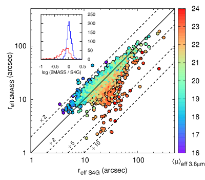
Figure 16.— Comparison between the 2MASS XSC effective radii and the S⁴G ones. For each galaxy, the 2MASS radius is the average of the effective radii in $J$, $H$ and $K_{S}$. The S⁴G radii are measured at 3.6 $\micron$. The color code reflects the average surface brightness inside the effective radius at 3.6 $\micron$, without correcting for inclination, in AB mag arcsec^-2. The inset plot shows the logaritmic ratio of the 2MASS and S⁴G effective radii for galaxies with $\langle\mu\rangle_{\mathrm{eff}\,3.6}<21$ (blue histogram) and $>21$ (red histogram).

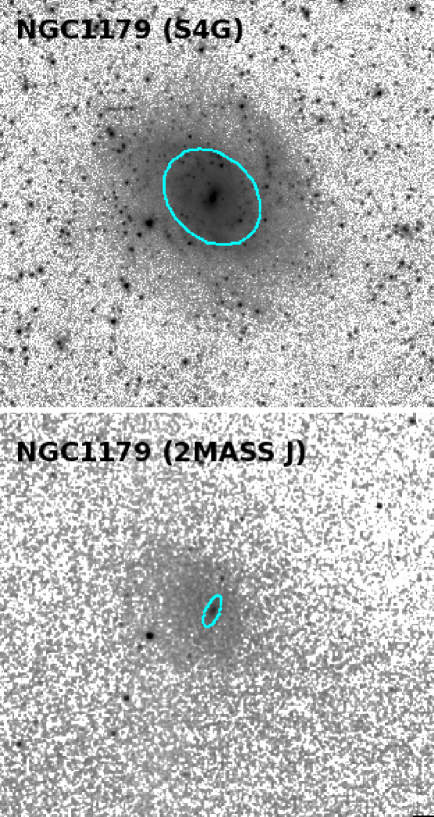
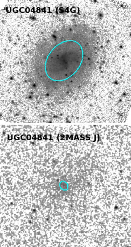
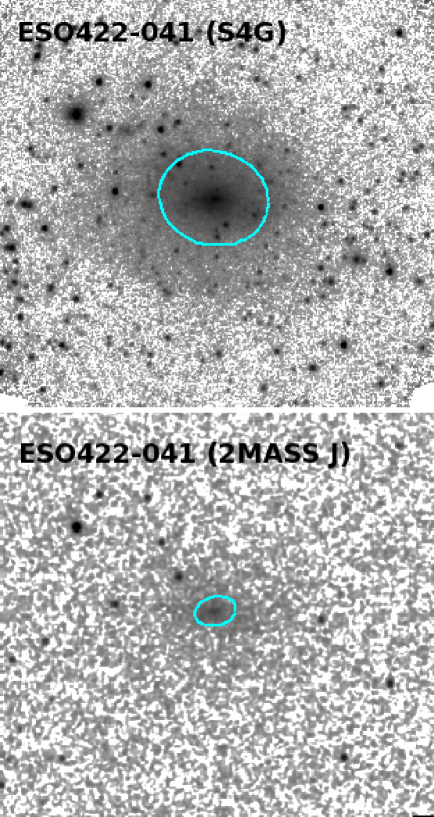
Figure 17.— Comparison of S⁴G 3.6 $\micron$ images (top) and 2MASS $J$ ones (bottom) for some representative galaxies with $\langle\mu\rangle_{\mathrm{eff}\,3.6}>21$ AB mag arcsec^-2. Images of the same galaxies are displayed at the same spatial scale. The cyan ellipses show the respective half-light apertures.

We can also compare our size measurements with those obtained from SDSS data using parametric fits, in order to understand how many components these fits must have in order to accurately recover the global non-parametric sizes of galaxies. The SDSS pipeline performs simple exponential or de Vaucouleurs fits to the light profiles of galaxies, but as we will show below these basic fits provide only rough (and potentially biased) estimates of galaxy sizes. More sophisticated fits, including Sérsic profiles and/or multi-component fits, have been widely used by other authors on SDSS data (see, e.g., Blanton et al. 2005; Gadotti 2009; Simard et al. 2011; Kelvin et al. 2012; Lackner & Gunn 2012).

Here we compare our effective radii with those measured by Lackner & Gunn (2012) on a sample of SDSS nearby galaxies, which includes 124 S⁴G objects. These authors fitted the $r$-band image of each galaxy with five different 2D models: a single exponential model, a single de Vaucouleurs one, a Sérsic model, an exponential bulge plus an exponential disk, and a de Vaucouleurs bulge plus an exponential disk.

We compare their effective radii along the major axis with the S⁴G ones in Fig. 18. Panels (a) to (e) show the five models described above, and panel (f) shows the model deemed by Lackner & Gunn (2012) as the most representative for each particular galaxy. The $r$-band radii are systematically larger than the 3.6 $\micron$ ones by $\sim 0.07-0.08$ dex. This is quantitatively consistent with the wavelength dependence of $r_{\mathrm{eff}}$ found by Lange et al. (2014), due to color gradients. After accounting for this offset, in term of scatter the “best model” option in panel (f) provides the best agreement with our non-parametric sizes, with a 1$\sigma$ scatter of merely $\pm 0.07$ dex ($\pm 16$%). The bulge$+$disk models yield a similar accuracy. The Sérsic fit does a somewhat poorer job, recovering the non-parametric sizes within $\pm 22$%. For the single exponential fit, the scatter around the 1:1 line is broader and more skewed, as such model is only suitable for almost bulgeless systems. Finally, the de Vaucouleurs profile completely overestimates the sizes except for some compact objects.

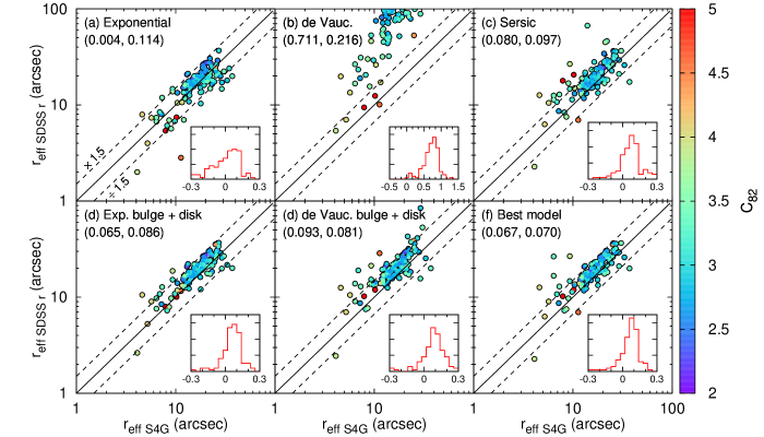
Figure 18.— SDSS $r$-band effective radii from Lackner & Gunn (2012) compared to the S⁴G ones at 3.6 $\micron$. The Lackner radii result from fitting each galaxy with various 2D models: (a) single exponential profile; (b) single de Vaucouleurs profile (the full range is not shown to avoid unnecessarily rescaling the axes of the other panels); (c) single Sérsic profile; (d) exponential bulge $+$ exponential disk; (e) de Vaucouleurs bulge $+$ exponential disk; (f) model that best describes each galaxy. Points are color-coded according to the 3.6 $\micron$ concentration index $C_{82}$. The small histograms show the distribution of $\log(r_{\mathrm{eff\,SDSS\,r}}/r_{\mathrm{eff\,S4G}})$. The mean and 1$\sigma$ values of these distributions are quoted in dex units as $(\mu,\sigma)$ in each panel.

7. Ancillary data and online access

The enhanced data products from our different pipelines are available through a dedicated webpage at the NASA/IPAC Infrared Science Archive. For each galaxy, users can download the P1 images and weight-maps, the P2 masks, the P3 radial profiles, the P4 GALFIT decompositions, and the P5 stellar mass maps.

IRSA also hosts an interactive catalog that contains all the global properties measured in P3 for each galaxy: central coordinates, background level and noise, outer isophotal sizes and shapes, apparent and absolute asymptotic magnitudes, stellar masses, and concentration indices. We have also incorporated into this catalog other parameters mined from external sources. In particular, the catalog contains redshift-independent distances from NED, and a variety of ancillary measurements compiled in HyperLeda such as optical sizes, magnitudes and colors, radial velocities, gas content and internal kinematics. This allows users to define detailed subsamples within S⁴G according to different selection criteria; the resulting list of galaxies can be then fed into the IRSA query system to retrieve the images, profiles and other data for the selected objects.

8. Summary

S⁴G is the largest and most homogeneous inventory of the stellar mass and structure in the nearby universe. Our 3.6 $\micron$ and 4.5 $\micron$ data peer through dust at the old stellar backbone of more than 2300 nearby galaxies of all morphological types in different environments.

In this paper we have described the methodology and algorithms of two of the pipelines in our data flow. Pipeline 2 creates masks of foreground stars and background galaxies. Pipeline 3 measures the background level and noise, performs surface photometry on the images, and derives global quantities such as asymptotic magnitudes, stellar masses, isophotal sizes and shapes, and concentration indices.

We find a structural transition between disk-dominated to bulge-dominated galaxies at stellar masses between $10^{10}$ and $10^{11}\,M_{\sun}$, concurrent with a drop in the specific SFR from $\sim 10^{-10.5}\,\mathrm{yr}^{-1}$ to $\sim 10^{-11.5}\,\mathrm{yr}^{-1}$ with increasing concentration. However, we find that not all galaxies with high stellar concentration indices are quiescent spheroidal systems. Bars and mergers can yield central concentrations of stellar mass while at the same time enhancing the overall SFR of the galaxy. Extended UV disks can also increase the SFR in the outer disk of galaxies that look otherwise compact in the IRAC bands.

We have also studied the local stellar-mass size relation at 3.6 $\micron$, which is consistent with previous results, but has the advantage of being little influenced by gradients in dust extinction or stellar age and metallicity. Early-type galaxies present an approximately constant stellar mass surface density of $10^{9}\,M_{\sun}\,\mathrm{kpc}^{-2}$. In late-type galaxies the surface density decreases with mass from $10^{9}\,M_{\sun}\,\mathrm{kpc}^{-2}$ to $10^{7}\,M_{\sun}\,\mathrm{kpc}^{-2}$.

Given the large ancillary value of S⁴G, we have made our enhanced data products available to the community through a dedicated webpage at IRSA. This data release includes not only the products described in the present paper (masks, radial profiles and derived global quantities), but also other enhanced products from our various pipelines, including science-ready mosaics and weight-maps, 2D image decompositions, and stellar mass maps.

Appendix A Pipeline 1 technical details

The S⁴G Pipeline 1 is an evolved version of the IRAC pipeline used for the SINGS Legacy Program (Kennicutt et al. 2003). A major change to the code from previous versions is the removal of a step to improve the registration of individual frames using cross-correlation, because the Spitzer calibration now uses 2MASS to improve the astrometry. Also, sky subtraction has been moved into Pipeline 3. Below we summarize the steps in the pipeline.

A.1. Saturation removal and rough cosmic ray rejection

The first step is optional and only occurs when the IRAC observations were taken in High Dynamic Range (HDR) mode. In this mode a short exposure is taken before the main exposure at each location. For the vast majority of the observations in the sample, the main observation is 30 seconds and the HDR exposure is 1.2 seconds. For new galaxies that were only observed during the warm mission we did not use HDR mode since very few have bright nuclei.

If the Basic Calibrated Data (BCD) images have an HDR counterpart and the flux in the pixel is above $10^{6}$ MJy sr^-1, the value from the normal BCD is replaced by the HDR one. In addition, we do a rough cosmic ray removal by replacing the value of the pixels in the normal BCD image with the value in the HDR pixel when the difference is above 3 MJy sr^-1.

A.2. Optical distortion correction and rotation

Before we can compare the sky level in overlapping BCD images, we must first correct each BCD for optical distortion and rotate the images to have the same orientation. This is required to get pixels to all have the same projeted size and orientation on the sky. To do this we use the Drizzle routine and create a new optically corrected BCD image for each BCD image in the mosaic. Once we have all the images with constant size on the sky we can find the matching regions of overlap.

A.3. Determining the background offset between BCD images

For all pairs of overlapping BCD images where at least a minimum number of pixels (nominally 20,000) overlap between the two images we find the background offset. To determine the background offset we find the difference in the 20th percentile pixel flux in both images. Using the 20th percentile has several advantages over a mean or median. Our goal is to find the change in the background level rather than any changes when pixels receive flux from resolved sources. Sub-pixel changes in the telescope position will change the flux level of pixels observing a point source substantially with the IRAC undersampled optics. These same sub-pixel changes do not affect the observations of the unresolved background. Also, some detector artifacts such as mux bleed and column pull down can affect large areas leading to biases in even the median, while using the 20th percentile value minimizes the bias.

For some archive observations the original frames had minimal overlap for the mosaic. In those cases we had to reduce the required number of pixels in the overlap region to be as low as 5000.

A.4. Solving for the background offset correction

Once we have the background offset between each pair of overlapping BCD images, we used the method of Regan & Gruendl (1995) to find the background offset for each image that minimizes the residuals. This method performs a least square minimization of the residuals using a single offset that is applied to each image.

Due to their small size, many sample galaxies were not observed in IRAC mapping mode but instead were observed in dither mode. In this case two (or even three) non-overlapping regions of the sky are observed and there is a need of additional information to obtain a solution. Therefore, when the regions of the sky do not overlap we add in an offset between a BCD image in each region of the sky. This will force the sky level to be similar between the non-overlapping regions of the sky.

The set of measured offsets of overlapping images does not provide a zero point for the solution, which requires having an external paramenter fixed to set the zero point for the relative offsets. To minimize the effect of applying the offsets on the background level, we place the additional constraint that the average offset should have a value of 0. Once we know the correction that needs to be applied, we create a corrected version of each input BCD image.

A.5. Drizzle the corrected images and update FITS header

The final mosaics are created using the standard STDAS PYRAF task Drizzle. The resuling images have a plate scale of 0.75″ per pixel and are oriented to have north to the top. We have to make a correction to the output of the drizzling task to recover the correct photometry. Drizzle assumes the pixels have units of flux instead of surface brightness. We apply a correction to account for the smaller pixel area in the final mosaic. Drizzle also returns a weight map that shows the number of seconds of integration time for each final pixel. This image is also included in the S⁴G archive and is used by subsequent S⁴G pipelines.

In the final step we update the FITS header to include a list of the Astronomical Observation Requests (AORs) that contributed to the final mosaic and set all the pixels outside of the field of view to have the value of NAN.

References

- Aaronson et al. (1979) Aaronson, M., Huchra, J., & Mould, J. 1979, ApJ, 229, 1
- Abraham et al. (1996a) Abraham, R. G., Tanvir, N. R., Santiago, B. X., et al. 1996a, MNRAS, 279, L47
- Abraham et al. (1996b) Abraham, R. G., van den Bergh, S., Glazebrook, K., et al. 1996b, ApJS, 107, 1
- Abraham et al. (2003) Abraham, R. G., van den Bergh, S., & Nair, P. 2003, ApJ, 588, 218
- Baggett et al. (1998) Baggett, W. E., Baggett, S. M., & Anderson, K. S. J. 1998, AJ, 116, 1626
- Barden et al. (2005) Barden, M., Rix, H.-W., Somerville, R. S., et al. 2005, ApJ, 635, 959
- Bell & de Jong (2000) Bell, E. F., & de Jong, R. S. 2000, MNRAS, 312, 497
- Bell & de Jong (2001) —. 2001, ApJ, 550, 212
- Bender et al. (1988) Bender, R., Doebereiner, S., & Moellenhoff, C. 1988, A&AS, 74, 385
- Bershady et al. (2000) Bershady, M. A., Jangren, A., & Conselice, C. J. 2000, AJ, 119, 2645
- Bertin & Arnouts (1996) Bertin, E., & Arnouts, S. 1996, A&AS, 117, 393
- Blanton et al. (2005) Blanton, M. R., Schlegel, D. J., Strauss, M. A., et al. 2005, AJ, 129, 2562
- Bosma (1978) Bosma, A. 1978, PhD thesis, PhD Thesis, Groningen Univ., (1978)
- Brinchmann et al. (2004) Brinchmann, J., Charlot, S., White, S. D. M., et al. 2004, MNRAS, 351, 1151
- Busko (1996) Busko, I. C. 1996, in Astronomical Society of the Pacific Conference Series, Vol. 101, Astronomical Data Analysis Software and Systems V, ed. G. H. Jacoby & J. Barnes, 139
- Calzetti (2001) Calzetti, D. 2001, PASP, 113, 1449
- Caon et al. (1993) Caon, N., Capaccioli, M., & D’Onofrio, M. 1993, MNRAS, 265, 1013
- Carter (1978) Carter, D. 1978, MNRAS, 182, 797
- Comerón et al. (2011) Comerón, S., Elmegreen, B. G., Knapen, J. H., et al. 2011, ApJ, 741, 28
- Comerón et al. (2013) Comerón, S., Salo, H., Laurikainen, E., et al. 2013, ArXiv e-prints, arXiv:1312.0866
- Conselice (2003) Conselice, C. J. 2003, ApJS, 147, 1
- Conselice et al. (2003) Conselice, C. J., Bershady, M. A., Dickinson, M., & Papovich, C. 2003, AJ, 126, 1183
- Courteau et al. (2007) Courteau, S., Dutton, A. A., van den Bosch, F. C., et al. 2007, ApJ, 671, 203
- Dale et al. (2009) Dale, D. A., Cohen, S. A., Johnson, L. C., et al. 2009, ApJ, 703, 517
- de Blok et al. (2008) de Blok, W. J. G., Walter, F., Brinks, E., et al. 2008, AJ, 136, 2648
- de Jong (1996) de Jong, R. S. 1996, A&A, 313, 377
- de Vaucouleurs (1977) de Vaucouleurs, G. 1977, in Evolution of Galaxies and Stellar Populations, ed. B. M. Tinsley & R. B. Larson, 43–+
- de Vaucouleurs et al. (1991) de Vaucouleurs, G., de Vaucouleurs, A., Corwin, Jr., H. G., et al. 1991, Third Reference Catalogue of Bright Galaxies. Volume I: Explanations and references. Volume II: Data for galaxies between 0h and 12h. Volume III: Data for galaxies between 12h and 24h.
- Driver et al. (2011) Driver, S. P., Hill, D. T., Kelvin, L. S., et al. 2011, MNRAS, 413, 971
- Epchtein et al. (1994) Epchtein, N., de Batz, B., Copet, E., et al. 1994, Ap&SS, 217, 3
- Erwin (2005) Erwin, P. 2005, MNRAS, 364, 283
- Eskew et al. (2012) Eskew, M., Zaritsky, D., & Meidt, S. 2012, AJ, 143, 139
- Eskridge et al. (2000) Eskridge, P. B., Frogel, J. A., Pogge, R. W., et al. 2000, AJ, 119, 536
- Eskridge et al. (2002) —. 2002, ApJS, 143, 73
- Fall & Efstathiou (1980) Fall, S. M., & Efstathiou, G. 1980, MNRAS, 193, 189
- Fazio et al. (2004) Fazio, G. G., Hora, J. L., Allen, L. E., et al. 2004, ApJS, 154, 10
- Fernández Lorenzo et al. (2013) Fernández Lorenzo, M., Sulentic, J., Verdes-Montenegro, L., & Argudo-Fernández, M. 2013, MNRAS, 434, 325
- Franx et al. (2008) Franx, M., van Dokkum, P. G., Schreiber, N. M. F., et al. 2008, ApJ, 688, 770
- Fruchter & Hook (2002) Fruchter, A. S., & Hook, R. N. 2002, PASP, 114, 144
- Gadotti (2009) Gadotti, D. A. 2009, MNRAS, 393, 1531
- Gil de Paz & Madore (2005) Gil de Paz, A., & Madore, B. F. 2005, ApJS, 156, 345
- Gil de Paz et al. (2005) Gil de Paz, A., Madore, B. F., Boissier, S., et al. 2005, ApJ, 627, L29
- Gil de Paz et al. (2007) Gil de Paz, A., Boissier, S., Madore, B. F., et al. 2007, ApJS, 173, 185
- Hauser et al. (1998) Hauser, M. G., Arendt, R. G., Kelsall, T., et al. 1998, ApJ, 508, 25
- Ho et al. (2011) Ho, L. C., Li, Z.-Y., Barth, A. J., Seigar, M. S., & Peng, C. Y. 2011, ApJS, 197, 21
- Holwerda et al. (2011) Holwerda, B. W., Pirzkal, N., de Blok, W. J. G., et al. 2011, MNRAS, 416, 2401
- Holwerda et al. (2013) Holwerda, B. W., Munoz-Mateos, J., Comeron, S., et al. 2013, ArXiv e-prints, arXiv:1309.1444
- Holwerda et al. (2014) Holwerda, B. W., Muñoz-Mateos, J.-C., Comerón, S., et al. 2014, ApJ, 781, 12
- Jarrett et al. (2000) Jarrett, T. H., Chester, T., Cutri, R., et al. 2000, AJ, 119, 2498
- Jarrett et al. (2003) Jarrett, T. H., Chester, T., Cutri, R., Schneider, S. E., & Huchra, J. P. 2003, AJ, 125, 525
- Jedrzejewski (1987) Jedrzejewski, R. I. 1987, MNRAS, 226, 747
- Jogee et al. (2004) Jogee, S., Barazza, F. D., Rix, H.-W., et al. 2004, ApJ, 615, L105
- Kauffmann et al. (2003) Kauffmann, G., Heckman, T. M., White, S. D. M., et al. 2003, MNRAS, 341, 54
- Kelvin et al. (2012) Kelvin, L. S., Driver, S. P., Robotham, A. S. G., et al. 2012, MNRAS, 421, 1007
- Kennicutt (1998) Kennicutt, Jr., R. C. 1998, ARA&A, 36, 189
- Kennicutt et al. (2003) Kennicutt, Jr., R. C., Armus, L., Bendo, G., et al. 2003, PASP, 115, 928
- Kent (1985) Kent, S. M. 1985, ApJS, 59, 115
- Kim et al. (2014) Kim, T., Gadotti, D. A., Sheth, K., et al. 2014, ApJ, 782, 64
- Knapen et al. (2000) Knapen, J. H., Shlosman, I., & Peletier, R. F. 2000, ApJ, 529, 93
- Kormendy & Bender (1996) Kormendy, J., & Bender, R. 1996, ApJ, 464, L119
- Kormendy et al. (2009) Kormendy, J., Fisher, D. B., Cornell, M. E., & Bender, R. 2009, ApJS, 182, 216
- Kormendy & Kennicutt (2004) Kormendy, J., & Kennicutt, Jr., R. C. 2004, ARA&A, 42, 603
- Lackner & Gunn (2012) Lackner, C. N., & Gunn, J. E. 2012, MNRAS, 421, 2277
- Lange et al. (2014) Lange, R., Driver, S. P., Robotham, A. S. G., et al. 2014, ArXiv e-prints, arXiv:1411.6355
- Laurikainen et al. (2011) Laurikainen, E., Salo, H., Buta, R., & Knapen, J. H. 2011, MNRAS, 418, 1452
- Li & Draine (2001) Li, A., & Draine, B. T. 2001, ApJ, 554, 778
- Lotz et al. (2004) Lotz, J. M., Primack, J., & Madau, P. 2004, AJ, 128, 163
- MacArthur et al. (2004) MacArthur, L. A., Courteau, S., Bell, E., & Holtzman, J. A. 2004, ApJS, 152, 175
- MacArthur et al. (2003) MacArthur, L. A., Courteau, S., & Holtzman, J. A. 2003, ApJ, 582, 689
- Marinova & Jogee (2007) Marinova, I., & Jogee, S. 2007, ApJ, 659, 1176
- Martín-Navarro et al. (2012) Martín-Navarro, I., Bakos, J., Trujillo, I., et al. 2012, MNRAS, 427, 1102
- Meidt et al. (2012) Meidt, S. E., Schinnerer, E., Knapen, J. H., et al. 2012, ApJ, 744, 17
- Meidt et al. (2014) Meidt, S. E., Schinnerer, E., van de Ven, G., et al. 2014, ApJ, 788, 144
- Menéndez-Delmestre et al. (2007) Menéndez-Delmestre, K., Sheth, K., Schinnerer, E., Jarrett, T. H., & Scoville, N. Z. 2007, ApJ, 657, 790
- Minchev et al. (2011) Minchev, I., Famaey, B., Combes, F., et al. 2011, A&A, 527, A147
- Mo et al. (1998) Mo, H. J., Mao, S., & White, S. D. M. 1998, MNRAS, 295, 319
- Morgan (1958) Morgan, W. W. 1958, PASP, 70, 364
- Muñoz-Mateos et al. (2011) Muñoz-Mateos, J. C., Boissier, S., Gil de Paz, A., et al. 2011, ApJ, 731, 10
- Muñoz-Mateos et al. (2007) Muñoz-Mateos, J. C., Gil de Paz, A., Boissier, S., et al. 2007, ApJ, 658, 1006
- Muñoz-Mateos et al. (2009a) Muñoz-Mateos, J. C., Gil de Paz, A., Zamorano, J., et al. 2009a, ApJ, 703, 1569
- Muñoz-Mateos et al. (2009b) Muñoz-Mateos, J. C., Gil de Paz, A., Boissier, S., et al. 2009b, ApJ, 701, 1965
- Muñoz-Mateos et al. (2013) Muñoz-Mateos, J. C., Sheth, K., Gil de Paz, A., et al. 2013, ApJ, 771, 59
- Paturel et al. (2003) Paturel, G., Petit, C., Prugniel, P., et al. 2003, A&A, 412, 45
- Peletier et al. (1990) Peletier, R. F., Davies, R. L., Illingworth, G. D., Davis, L. E., & Cawson, M. 1990, AJ, 100, 1091
- Peng et al. (2002) Peng, C. Y., Ho, L. C., Impey, C. D., & Rix, H.-W. 2002, AJ, 124, 266
- Peng et al. (2010) —. 2010, AJ, 139, 2097
- Querejeta et al. (2014) Querejeta, M., Meidt, S. E., Schinnerer, E., et al. 2014, ArXiv e-prints, arXiv:1410.0009
- Regan & Gruendl (1995) Regan, M. W., & Gruendl, R. A. 1995, in Astronomical Society of the Pacific Conference Series, Vol. 77, Astronomical Data Analysis Software and Systems IV, ed. R. A. Shaw, H. E. Payne, & J. J. E. Hayes, 335
- Regan et al. (1999) Regan, M. W., Sheth, K., & Vogel, S. N. 1999, ApJ, 526, 97
- Roškar et al. (2008) Roškar, R., Debattista, V. P., Stinson, G. S., et al. 2008, ApJ, 675, L65
- Rubin et al. (1978) Rubin, V. C., Thonnard, N., & Ford, Jr., W. K. 1978, ApJ, 225, L107
- Ryden (1992) Ryden, B. 1992, ApJ, 396, 445
- Ryden (2004) Ryden, B. S. 2004, ApJ, 601, 214
- Ryden (2006) —. 2006, ApJ, 641, 773
- Salo et al. (2015) Salo, H., Laurikainen, E., Laine, J., et al. 2015, ArXiv e-prints, arXiv:1503.06550
- Sánchez-Blázquez et al. (2009) Sánchez-Blázquez, P., Courty, S., Gibson, B. K., & Brook, C. B. 2009, MNRAS, 398, 591
- Sandage et al. (1970) Sandage, A., Freeman, K. C., & Stokes, N. R. 1970, ApJ, 160, 831
- Schlegel et al. (1998) Schlegel, D. J., Finkbeiner, D. P., & Davis, M. 1998, ApJ, 500, 525
- Scodeggio et al. (2002) Scodeggio, M., Gavazzi, G., Franzetti, P., et al. 2002, A&A, 384, 812
- Shen et al. (2003) Shen, S., Mo, H. J., White, S. D. M., et al. 2003, MNRAS, 343, 978
- Sheth et al. (2000) Sheth, K., Regan, M. W., Vogel, S. N., & Teuben, P. J. 2000, ApJ, 532, 221
- Sheth et al. (2005) Sheth, K., Vogel, S. N., Regan, M. W., Thornley, M. D., & Teuben, P. J. 2005, ApJ, 632, 217
- Sheth et al. (2008) Sheth, K., Elmegreen, D. M., Elmegreen, B. G., et al. 2008, ApJ, 675, 1141
- Sheth et al. (2010) Sheth, K., Regan, M., Hinz, J. L., et al. 2010, PASP, 122, 1397
- Simard et al. (2011) Simard, L., Mendel, J. T., Patton, D. R., Ellison, S. L., & McConnachie, A. W. 2011, ApJS, 196, 11
- Skrutskie et al. (2006) Skrutskie, M. F., Cutri, R. M., Stiening, R., et al. 2006, AJ, 131, 1163
- Sofue & Rubin (2001) Sofue, Y., & Rubin, V. 2001, ARA&A, 39, 137
- Sorce et al. (2012) Sorce, J. G., Courtois, H. M., & Tully, R. B. 2012, AJ, 144, 133
- Taylor et al. (2005) Taylor, V. A., Jansen, R. A., Windhorst, R. A., Odewahn, S. C., & Hibbard, J. E. 2005, ApJ, 630, 784
- Taylor-Mager et al. (2007) Taylor-Mager, V. A., Conselice, C. J., Windhorst, R. A., & Jansen, R. A. 2007, ApJ, 659, 162
- Thilker et al. (2005) Thilker, D. A., Bianchi, L., Boissier, S., et al. 2005, ApJ, 619, L79
- Thilker et al. (2007) Thilker, D. A., Boissier, S., Bianchi, L., et al. 2007, ApJS, 173, 572
- Trujillo et al. (2004) Trujillo, I., Rudnick, G., Rix, H.-W., et al. 2004, ApJ, 604, 521
- Trujillo et al. (2006) Trujillo, I., Förster Schreiber, N. M., Rudnick, G., et al. 2006, ApJ, 650, 18
- Tully & Fisher (1977) Tully, R. B., & Fisher, J. R. 1977, A&A, 54, 661
- van der Wel et al. (2014) van der Wel, A., Franx, M., van Dokkum, P. G., et al. 2014, ApJ, 788, 28
- Verheijen (2001) Verheijen, M. A. W. 2001, ApJ, 563, 694
- Wang et al. (2011) Wang, J., Kauffmann, G., Overzier, R., et al. 2011, MNRAS, 412, 1081
- Werner et al. (2004) Werner, M. W., Roellig, T. L., Low, F. J., et al. 2004, ApJS, 154, 1
- Whyte et al. (2002) Whyte, L. F., Abraham, R. G., Merrifield, M. R., et al. 2002, MNRAS, 336, 1281
- Wright et al. (2010) Wright, E. L., Eisenhardt, P. R. M., Mainzer, A. K., et al. 2010, AJ, 140, 1868
- York et al. (2000) York, D. G., Adelman, J., Anderson, Jr., J. E., et al. 2000, AJ, 120, 1579
- Younger et al. (2007) Younger, J. D., Cox, T. J., Seth, A. C., & Hernquist, L. 2007, ApJ, 670, 269
- Zaritsky et al. (2013) Zaritsky, D., Salo, H., Laurikainen, E., et al. 2013, ApJ, 772, 135
- Zaritsky et al. (2014) Zaritsky, D., Courtois, H., Muñoz-Mateos, J.-C., et al. 2014, AJ, 147, 134