Halo detection via large-scale Bayesian inference

Abstract

We present a proof-of-concept of a novel and fully Bayesian methodology designed to detect halos of different masses in cosmological observations subject to noise and systematic uncertainties. Our methodology combines the previously published Bayesian large-scale structure inference algorithm, HADES, and a Bayesian chain rule (the Blackwell-Rao Estimator), which we use to connect the inferred density field to the properties of dark matter halos. To demonstrate the capability of our approach we construct a realistic galaxy mock catalogue emulating the wide-area 6-degree Field Galaxy Survey, which has a median redshift of approximately 0.05. Application of HADES to the catalogue provides us with accurately inferred three-dimensional density fields and corresponding quantification of uncertainties inherent to any cosmological observation. We then use a cosmological simulation to relate the amplitude of the density field to the probability of detecting a halo with mass above a specified threshold. With this information we can sum over the HADES density field realisations to construct maps of detection probabilities and demonstrate the validity of this approach within our mock scenario. We find that the probability of successful of detection of halos in the mock catalogue increases as a function of the signal-to-noise of the local galaxy observations. Our proposed methodology can easily be extended to account for more complex scientific questions and is a promising novel tool to analyse the cosmic large-scale structure in observations.

Halo detection via Bayesian inference

1 Introduction

The dual role of galaxy clusters, both as cosmological probes and as unique sites for studying extreme environments of galaxy formation, make them essential targets for next generation cosmological galaxy surveys (e.g. see Borgani & Guzzo 2001; Borgani et al. 2001; Rosati et al. 2002; Voit 2005; Allen et al. 2011 and Kravtsov & Borgani 2012). Ongoing and next generation cosmological surveys, including, for example, the Dark Energy Survey (The Dark Energy Survey Collaboration, 2005), the Large Synoptic Survey Telescope (Ivezic et al., 2008), the Euclid mission (Laureijs et al., 2011), the Javalambre-Physics of the Accelerated Universe Astrophysical Survey (J-PAS, Benitez et al., 2014) and the eROSITA mission (Merloni et al., 2012), are expected to observe many thousands of galaxy clusters out to redshifts beyond $z\sim 1$.

As such there is great demand for cluster-finding algorithms that remain robust, reliable and efficient out to high redshift and for catalogues of varying degrees of incompleteness. Many different methods exist for detecting galaxy clusters in optical/near-infrared selected surveys, as well as other approaches based on measurements of X-ray emission (e.g. Ebeling et al., 2000; Rosati et al., 2002; Böhringer et al., 2004), weak gravitational lensing (e.g. Tyson et al., 1990; Bartelmann & Schneider, 2001; Leonard et al., 2014) or the Sunyaev-Zeldovich effect (e.g. Sunyaev & Zeldovich, 1972; Carlstrom et al., 2002; Ascaso & Moles, 2007).

For cluster detection in optical or near-infrared datasets, several techniques have been developed, which can be classified broadly into three groups according to the galaxy information that they primarily rely on. First are those approaches based primarily upon the spatial extent of the cluster galaxies, such as the Counts-in-Cells technique (e.g. Couch et al., 1991; Lidman & Peterson, 1996), Percolation algorithms (e.g. Huchra & Geller, 1982; Dalton et al., 1997; Eke et al., 2004; Ramella et al., 2002; Robotham et al., 2011) and the Voronoi-Delauney method (e.g. Ramella et al., 2001; Marinoni et al., 2002; Kim et al., 2002), which identify clusters as density enhancements over the mean background. The chief strength of these algorithms is their simplicity, namely their lack of assumptions regarding cluster shapes and their ability to work with single-band selections. Their sensitivity to line-of-sight positions, however, typically limits their use to spectroscopic surveys, though there have been some attempts to apply such algorithms to photometric datasets (e.g. Botzler et al., 2004; Farrens et al., 2011; Jian et al., 2014).

Second are the detection techniques that instead identify cluster candidates through the presence of a red sequence; the population of red, elliptical galaxies in clusters, typically thought to have had their star-formation quenched by feedback processes. Assuming that the cluster galaxy population is dominated by early-type galaxies and that this population follows a tight colour-magnitude relation with little intrinsic scatter, then, when imaged in two photometric bands bracketing the $4000{\rm\AA}$ break, the cluster red sequence galaxies will be the brightest, reddest objects (Stanford et al., 1998; Gladders & Yee, 2000). By dividing the colour-space into slices (according to a red sequence model) and assigning a weight to each galaxy based upon the likelihood that the galaxy belongs to particular slice, one can construct a surface density map for each slice, with the peaks in the density corresponding to the cluster candidates. Examples include the Cluster Red Sequence method (Gladders & Yee, 2000; López-Cruz et al., 2004; Gladders & Yee, 2005), the Cut-and-Enhance algorithm (Goto et al., 2002), the MaxBCG algorithm (Hansen et al., 2005; Koester et al., 2007), the C4 algorithm (Miller et al., 2005), the ORCA algorithm (Murphy et al., 2012) and the redMaPPer algorithm (Rykoff et al., 2014). These algorithms are popular choices for use with photometric datasets, though there is the obvious concern that such algorithms are biased towards those clusters with an established red sequence.

Finally, are the techniques that model characteristics of clusters, such as the spatial or luminosity distribution of galaxies in clusters, and test how well the galaxies in a particular region of the sky match this model. For example, the Matched Filter technique (Postman et al., 1996), models the distribution of galaxies within a cluster as a sum of the background density and a parametrised function of the cluster galaxy luminosity function and the projected radial profile of the cluster. One can then determine a likelihood for the model parameters as a function of redshift and luminosity. Maximising the likelihoods can therefore provide estimates for the redshift and the total luminosity of a cluster. Several extensions to the Matched Filter have been proposed, including the Adaptive Matched Filter (Kepner et al., 1999), the Hybrid Matched Filter (Kim et al., 2002) and the three-dimensional Matched Filter (Milkeraitis et al., 2010). Recently, Ascaso et al. (2012) implemented a variation of the matched filter technique in a Bayesian framework in order to assign to each galaxy a Bayesian probability that there is a cluster centred on that galaxy. By additionally introducing an optional prior for the presence of a cluster red sequence, they were able to demonstrate the recovery of clusters with a red sequence without the need for colour-magnitude modelling. Matched filter methods are typically powerful techniques capable of recovering clusters in deep, photometric redshift surveys with high completeness and little contamination. However, their reliance on models for the luminosity and radial profiles of clusters suggests that their results could be model dependent and biased towards clusters displaying similar characteristics.

In this work we describe a novel and fully Bayesian approach to detect halos with masses above specific thresholds as peaks in the smooth matter density field inferred from observations. To achieve this goal we capitalise on, firstly, the previously developed HADES (Jasche & Kitaura, 2010; Jasche & Wandelt, 2012) large-scale structure inference framework, which is designed to infer, from observations, the smooth three-dimensional matter density field of the cosmic large-scale structure, and, secondly, the Blackwell-Rao Estimator, which we use to relate the inferred density amplitudes to the properties of dark matter halos. Our framework exploits information from the entirety of a galaxy survey and makes no assumptions regarding the spatial extent of clusters, the functional form of their radial profiles or the presence of a red sequence, which can be affected by cosmic variance. Instead our method relies upon the more fundamental assumption of our understanding of the matter power spectrum, which can in turn be sampled self-consistently as part of the Bayesian framework (see e.g. Jasche et al., 2010b; Jasche & Wandelt, 2013b; Jasche & Lavaux, 2015). To examine the success of our methodology we make use of a realistic mock galaxy catalogue for which halo memberships of the galaxies are known.

The layout of the paper is as follows. In $\S$2 we present the Bayesian inference framework HADES and describe our process for generating a realistic mock catalogue for the 6 degree Field Galaxy Survey (6dFGS). The inference of the three-dimensional density field for this dataset is described in $\S$3, followed by a discussion of inference results. In $\S$4 we describe our approach to detect halos of different masses in observations via a Blackwell-Rao methodology. Subsequently, we apply this approach to the inference results obtained by the application of HADES to the 6dFGS mock catalogue and estimate its performance to recover halos in a realistic, data driven scenario. Finally we summarise and draw conclusions in $\S$5. All magnitudes are in the Vega system. Details of the cosmological model that we adopt are given in $\S$2.2.1.

2 Methodology

In this section we first give a brief overview of the Bayesian inference algorithm, HADES, that we employ and then introduce the N-body simulation and the semi-analytical galaxy formation model, GALFORM, that we use to construct our mock galaxy catalogue.

2.1 The HADES algorithm

In this work we use the HAmiltonian Density Estimation and Sampling algorithm (HADES, Jasche & Kitaura, 2010; Jasche et al., 2010a; Jasche & Wandelt, 2012); a full scale Bayesian inference framework designed to analyse modern galaxy large-scale structure surveys on both linear and non-linear cosmic scales, whilst simultaneously providing the corresponding uncertainty quantification.

The three-dimensional large-scale structure of the cosmic web offers a wealth of valuable information for testing our current picture of cosmological structure and galaxy formation. However, connecting observations to theoretical predictions is not trivial. Observations of the large-scale structure are typically subject to a variety of systematic and statistical uncertainties, such as survey geometries, selection effects, galaxy biases, the noise of the galaxy distribution and cosmic variance. All these effects have to be carefully accounted for to ensure that we do not draw erroneous conclusions on the final inferred quantities. Additional complexity for the inference of the three-dimensional density field arises from the fact that in this work we seek to analyse the large-scale structure on scales of $\sim 4\,\,h^{-1}{\rm Mpc}$, in the mildly non-linear and non-linear regimes. At these scales the non-linearly evolved density field no longer obeys simple Gaussian statistics as gravitational interactions introduce mode coupling and phase correlations. Unfortunately there is no tractable solution, in the form of a fully multivariate probability distribution, for the non-linear three-dimensional density field. There exist, however, phenomenological approximations, such as the log-normal distribution.

The log-normal distribution can be justified via theoretical arguments, as shown by Coles & Jones (1991), and has been demonstrated to fit, with reasonable accuracy, the one-point distributions obtained from numerical large-scale structure simulations (Kayo et al., 2001). Using the log-normal distribution together with a suitable choice for the cosmic power spectrum to account for one- and two-point statistics of the density field is thus a logical choice for a prior distribution used in Bayesian inferences of the non-linear matter distribution. From an information theory perspective such a log-normal prior is well justified, since it is a maximum entropy prior on a logarithmic scale. This means that amongst all possible probability distributions with the same mean and covariance matrix on a logarithmic scale, the log-normal distribution is the distribution that contains the least information. As such the log-normal distribution represents the least informative prior for a positive three-dimensional density field, once the mean and covariance matrix are specified (Jasche & Kitaura, 2010; Jasche et al., 2010a).

To find a suitable likelihood distribution we note that the galaxy distribution is conditionally dependent on the underlying three-dimensional matter density field. In particular, in the most naive picture of galaxy formation, galaxies are predominantly found in regions of higher density than in regions of lower density. The local noise structure of the galaxy distribution is therefore dependent on the underlying matter density field. This feature of signal-dependent noise is missed in traditional approaches based on Gaussian approximations such as Wiener filtering (Fisher et al., 1994; Zaroubi et al., 1995; Erdoǧdu et al., 2004; Kitaura et al., 2009; Jasche et al., 2010b). Assuming galaxies to be discrete particles, their distribution can be described as a specific realisation drawn from an inhomogeneous Poisson process, which captures the essential features of such a signal dependent noise (see e.g. Layzer, 1956; Peebles, 1980; Martínez & Saar, 2002).

Consequently, analyses of the three-dimensional density field in the non-linear regime requires the solving of a large-scale Bayesian inverse problem with a log-normal Poisson distribution. To explore this highly non-Gaussian and non-linear problem the HADES algorithm relies on a Hybrid Monte-Carlo (HMC) scheme, which, instead of the random walk behaviour displayed by traditional Metropolis-Hastings algorithms, follows a persistent motion similar to particle trajectories in classical mechanics problems (see Jasche & Kitaura 2010 for a detailed discussion of the necessary equations of motion and their numerical implementation). Being a fully Bayesian method, the HADES algorithm does not only provide a single estimate of the density field but rather a full numerical representation of the large-scale structure posterior conditional on the observations, including a detailed treatment of all systematic and stochastic uncertainties. The output products from HADES are therefore a set of realisations of the three-dimensional density field in a voxel grid, as well as a measurement of the corresponding matter power spectrum. In this fashion, the algorithm permits determination of any desired statistical summary such as the mean, mode and variance and simultaneously provides a straightforward means to non-linearly propagate non-Gaussian uncertainties on any inferred quantity (Jasche & Kitaura, 2010; Jasche et al., 2010a).

Recently, the HADES algorithm has been extended to account for photometric redshift uncertainties by using a block sampling procedure (Jasche & Wandelt, 2012). This update means that HADES is able to account for the corresponding redshift uncertainties of millions of galaxies observed by photometric surveys, whilst simultaneously inferring an accurate representation of the three-dimensional density field from such datasets. For a more detailed overview of the Bayesian inference framework implemented in HADES the interested reader is referred to previous publications: Jasche & Kitaura (2010); Jasche et al. (2010a) and Jasche & Wandelt (2012).

2.2 Generating a mock catalogue

In order to demonstrate the capability of our approach to identify halos of galaxies, we apply HADES and our halo detection methodology to a synthetic mock galaxy catalogue in which halo memberships are known. This will allow us to quantify how well our approach can recover the original structures.

To this end we construct a mock catalogue to emulate the Six-degree Field Galaxy Survey (6dFGS, Jones et al., 2004), which was carried out between 2004 and 2009 using the 6-degree Field automated fibre positioner and spectrograph system (6dF, Parker et al., 1998; Watson et al., 2000) on the UK Schmidt Telescope at the Australian Astronomical Observatory (AAO). The 6dFGS is a near-infrared selected galaxy survey covering the whole of the Southern sky, approximately $17,000^{\circ}$, down to a galactic latitude of $|b|>10^{\circ}$. As of the final data release (DR3, Jones et al., 2009), the 6dFGS yielded a catalogue of approximately 125,000 extra-galactic redshifts complete to $\left({\rm K},{\rm H},{\rm J},{\rm r_{F}},{\rm b_{J}}\right)=(12.65,12.95,13.75,15.60,16.75)$. Here, we construct a mock catalogue to emulate the K-band selected sub-sample of the 6dFGS, which with approximately 93,000 redshifts constitutes the majority of the survey.

We choose to emulate the 6dFGS for several reasons. Firstly, the 6dFGS has a large sky coverage, with a close to uniform completeness across the majority of the survey area. Secondly, the shallow depth of the 6dFGS means that there is little structure evolution throughout the domain of the survey. As such, we are able to, in the first instance, demonstrate our halo detection methodology on a density field that is evolving very little with redshift. This means that we can approximate the matter density field throughout the mock catalogue using the $z=0$ snapshot of the MS-W7 Simulation (Guo et al., 2013). This allows us to provide a simple proof-of-concept of the approach. Future application of the methodology to deeper surveys, such as the Sloan Digital Sky Survey (SDSS, York et al., 2000), can then be achieved by incorporating a more sophisticated approach to model the redshift-dependence of the matter density field. Thirdly, we plan in future work to apply our approach to the real 6dFGS, which contains a rich variety of well-studied local structures, ranging from small groups, to large super-clusters such as the Shapley Super-cluster.

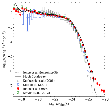
Figure 1: K-band luminosity function at $z=0$ for the idealised mock catalogue (solid black line). Also plotted for comparison are the 6dFGS K-band luminosity function estimate from Jones et al. (2006), as well as K-band luminosity function estimates from Kochanek et al. (2001), Cole et al. (2000) and Driver et al. (2012). The dotted line shows the Schechter (1976) functional fit to the 6dFGS luminosity function using the parameters from Jones et al. (2006).

2.2.1 Galaxy formation model

To construct a 6dFGS mock catalogue we follow a construction method similar to that of Merson et al. (2013), which involves first populating the dark matter halo merger trees of a cosmological N-body simulation with galaxies using a semi-analytical model.

The cosmological simulation that we use is the MS-W7 Simulation (Guo et al., 2013), which is a version of the Millennium Simulation (Springel et al., 2005) constructed using a cold dark matter (CDM) cosmology consistent with the 7-year results of the Wilkinson Microwave Anisotropy Probe (WMAP7, Komatsu et al., 2011). The cosmological parameters are: a baryon matter density $\Omega_{{\rm b}}=0.0455$, a total matter density $\Omega_{{\rm m}}=\Omega_{{\rm b}}+\Omega_{{\rm CDM}}=0.272$, a dark energy density $\Omega_{{\rm\Lambda}}=0.728$, a Hubble constant $H_{0}=100h\,{\rm km\,s}^{-1}{\,\rm Mpc}^{-1}$ where $h=0.704$, a primordial scalar spectral index $n_{\rm s}=0.967$ and a fluctuation amplitude $\sigma_{8}=0.810$.

The hierarchical growth of cold dark matter structure is followed at 62 fixed epoch snapshots, spaced approximately logarithmically in expansion factor between redshift $z=127$ and the present day, in a cubic volume of size $500\,h^{-1}{\,\rm Mpc}$ on a side. For each snapshot, groups of dark matter particles are first identified through the application of a friends-of-friends algorithm (Davis et al., 1985). The substructure-finder SUBFIND (Springel et al., 2001) is then applied to break these groups down into identifiable, self-bound sub-halos. Independent halos are determined by establishing a sub-halo hierarchy and identifying those sub-halos that are not bound by any more massive sub-halos. By tracking sub-halo descendants between the subsequent output snapshots a halo merger tree can be constructed. Further details regarding construction of the halo merger trees can be found in Merson et al. (2013) and Jiang et al. (2014). The MS-W7 simulation uses $2160^{3}$ particles to represent the matter distribution, with the requirement that a halo consists of at least 20 particles for it to be resolved. This corresponds to a halo mass resolution of $M_{{\rm halo,lim}}\simeq 1.87\times 10^{10}\,h^{-1}{\rm M_{\odot}}$, significantly smaller than expected for the Milky Way’s dark matter halo. (Within our chosen semi-analytical galaxy formation model, halos of this mass typically host galaxies with $M_{{\rm K}}-5\log_{10}(h)\sim-11.7$).

We model the star formation and merger history of galaxies using the GALFORM semi-analytical model of galaxy formation (Cole et al., 2000). Here we adopt the recent version presented by Gonzalez-Perez et al. (2014). The GALFORM model populates dark matter halos with galaxies using a set of coupled differential equations to determine how, over a given time-step, the “subgrid” physics regulates the size of the various baryonic components of galaxies. The physical processes modelled by GALFORM include: (i) the collapse and merging of dark matter (DM) halos, (ii) the shock-heating and radiative cooling of gas inside DM halos, leading to the formation of galactic discs (iii) quiescent star formation in galactic discs, (iv) feedback as a result of supernovae, active galactic nuclei and photo-ionisation of the inter-galactic medium, (v) chemical enrichment of stars and gas, (vi) dynamical friction driven mergers of galaxies within DM halos, capable of forming spheroids and triggering starburst events, and (vii) disk instabilities, which can also trigger starburst events. As detailed in Merson et al. (2013), how galaxies are placed into the dark matter halos depends on their status as central or satellite galaxies. Central galaxies are placed at the centre of the most massive sub-halo of their host halo. Following halo merger events, satellite galaxies are placed at the centre of mass of what was the most massive sub-halo of their original host halo when they were still a central galaxy. If this sub-halo can no longer be identified, the galaxy is placed on what was the most bound dark matter particle of that sub-halo. The GALFORM model is able to make predictions for numerous galaxy properties, including luminosities over a substantial wavelength range extending from the far-UV through to the sub-millimetre.

2.2.2 Catalogue construction

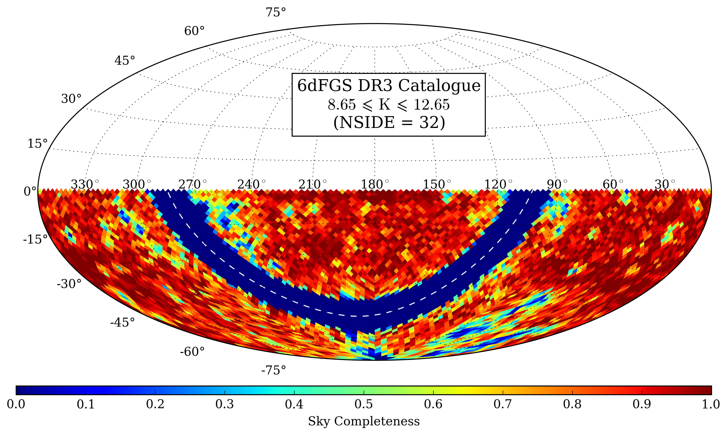
Figure 2: Redshift completeness as a function of sky position, $R(\mathbf{\theta})$, for the 6dFGS DR3 (in HEALPix format).

To construct the 6dFGS mock catalogue, we first run the GALFORM model on the $z=0$ snapshot of the MS-W7 simulation. An observer is then placed in the box at $(\mathrm{X_{o}},\mathrm{Y_{o}},\mathrm{Z_{o}})=(0,0,500)\,h^{-1}{\rm Mpc}$ and all galaxy positions are translated so that the observer is at the origin. To generate a cosmological volume comparable to that of the 6dFGS we stack a further three replications of the $z=0$ box such that we have a cuboid spanning, relative to the observer, $[-500,500]\,h^{-1}{\rm Mpc}$ in the X and Y directions and $[-500,0]\,h^{-1}{\rm Mpc}$ in the Z direction. Note that, given the cosmology of the simulation, a co-moving distance of $500\,h^{-1}{\rm Mpc}$ corresponds to a redshift $z\sim 0.17$.

We next apply the selections to mimic the 6dFGS. Firstly we use the Cartesian positions of each galaxy to compute a sky position and redshift for that galaxy. The cosmological redshift of the galaxy is calculated from the co-moving distance to the galaxy from the observer, $r_{\mathrm{com}}$, defined by,

$$r_{{\rm com}}(z)={\displaystyle\int^{z}_{0}\frac{c\,{\rm d}z^{\prime}}{H_{0}\sqrt{\Omega_{\rm m}\left(1+z^{\prime}\right)^{3}+\Omega_{{\rm\Lambda}}}}},$$ (1)

where $c$ is the speed of light. For the purposes of our HADES analysis we place an initial cut so that all galaxies with cosmological redshift $z>0.16$ are discarded. Note that this redshift is well beyond the median redshift of the 6dFGS, $z_{\mathrm{med}}\sim 0.05$. We calculate an observed redshift, $z_{\mathrm{obs}}$, of each galaxy using,

$$z_{{\rm obs}}=\left(1+z\right)\left(1+\frac{v_{{\rm r}}}{c}\right)-1,$$ (2)

where $v_{\mathrm{r}}$ is the radial component of the peculiar velocity vector, $\mathbf{\vec{v}}$, of the galaxy (i.e. $v_{{\rm r}}=\mathbf{\vec{v}}\cdot\mathbf{\hat{r}}$, where $\mathbf{\hat{r}}$ is the normalised line-of-sight position vector of the galaxy). Note that we do not incorporate any spectroscopic redshift uncertainties in the mock catalogue. To mimic the solid angle footprint of the 6dFGS we reject any galaxies with declination $\delta>0^{\circ}$ as well as those galaxies with a galactic latitude $|b|<10^{\circ}$.

The next step is to apply the K-band flux selection limit of the 6dFGS, ${\rm K}<12.65$, to reject those galaxies that are too faint to have been observed. The GALFORM model provides the absolute K-band magnitude, $\mathrm{M_{K}}-5\log_{10}(h)$, of each galaxy. We calculate the apparent K-band magnitude, $\mathrm{K}$, of each galaxy using,

$$\mathrm{K}=\mathrm{M_{K}}-5\log_{10}(h)+5\log_{10}\left(\frac{d_{L}\left(z\right)}{10{\rm pc}}\right)$$

$$-2.5\log_{10}\left(1+z\right)+k(z),$$ (3)

where $d_{L}$ is the luminosity distance to the galaxy and $k(z)$ is an applied K-band k-correction, which we obtain by interpolating the tabulated k-corrections from Poggianti (1997). In Fig. 1 we show the K-band luminosity function for the mock catalogue, which we compare with the 6dFGS K-band luminosity function estimated by Jones et al. (2006). Note that Jones et al. corrected their estimate of the 6dFGS luminosity function for incompleteness. Our mock catalogue gives a galaxy number density that is in excellent agreement with that of the 6dFGS, particularly around the characteristic magnitude, $\mathrm{M_{K}^{\ast}}-5\log_{10}(h)=-23.83$.

At this stage, the mock catalogue that we have represents an idealised copy of the 6dFGS, such that the catalogue is complete down to the flux limit and complete over the extent of the 6dFGS DR3 footprint on the sky. The final step is to degrade the completeness of our idealised mock catalogue such that we model the effect of systematics that are introduced into observational datasets as a result of survey strategy. For spectroscopic surveys such as the 6dFGS, incompleteness is introduced as a result of observational limitations, such as fibre collisions and effects of poor observing conditions, which prevent one from obtaining a redshift measurement for each target. Collisions of the 6dF fibres, for example, prevent simultaneous observation of galaxies with a proximity less than approximately $5.71$ arcminutes on the sky (Campbell et al., 2004), though this can be mitigated somewhat by repeat observations. Such systematics can therefore lead to the observed galaxy counts in any particular dark matter halo being incomplete, which reduces the signal-to-noise of that halo. Therefore it is important to ensure that we are applying our methodology to a mock dataset that is representative of observational datasets and their inherent systematics.

Jones et al. (2006) model the total completeness, $T(\boldsymbol{\theta},m)$, for each galaxy in the 6dFGS using the separable function $T(\boldsymbol{\theta},m)=S(\boldsymbol{\theta})C(m)$, where $C(m)$ is the completeness as a function of magnitude, $m$, and $S(\boldsymbol{\theta})$ is a constant scaling the completeness of the field in which a galaxy was observed to the completeness, $R(\boldsymbol{\theta})$, on that part of the sky. To remove incomplete regions from their final dataset, Jones et al. selected those galaxies for which $T(\boldsymbol{\theta},m)\geqslant 0.6$. In order to fully emulate the 6dFGS we would need to mimic the observational design of the survey, including optimally tiling the mock catalogue with a set of 6-degree fields and modelling effects such as fibre collision. However, given that the purpose of our mock catalogue is to help provide a simple demonstration of the ability of the our halo detection methodology and that to do this the mock catalogue does not need to be a perfect emulation, we choose to adopt a simpler, more straightforward implementation. We therefore degrade the mock catalogue using a HEALPix (Górski et al., 2005) realisation of the sky completeness mask of the DR3 dataset, as shown in Fig. 2, where the colour-bar indicates the value for the sky completeness $R(\boldsymbol{\theta})$, at the sky position, $\boldsymbol{\theta}$, of each HEALPix pixel. To degrade the mock catalogue we simply use random number generation to accept or reject galaxies based upon the value of $R(\boldsymbol{\theta})$ for the pixel to which the galaxy is assigned. By degrading the catalogue in this way, we ensure that the sky completeness mask in Fig. 2 is a good description for the completeness of the mock sky. Following this procedure, we are left with a mock catalogue that provides a reasonable approximation for a K-band selected 6dFGS-like galaxy survey. Note that our approach does not introduce any magnitude incompleteness, i.e. $C(m)=1$, and instead would lead to $T(\boldsymbol{\theta},m)=T(\boldsymbol{\theta})=R(\boldsymbol{\theta})$.

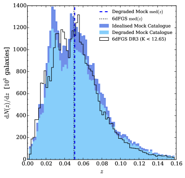
Figure 3: Redshift distributions for the idealised mock catalogue (dark blue shaded histogram) and the completeness degraded mock catalogue (light blue shaded histogram). Shown for comparison is the distribution for the 6dFGS DR3 K-band selected sample (black line). The dotted line indicates the median redshift for the 6dFGS DR3 galaxies, whilst the dashed line shows the median redshift for the degraded mock catalogue.

After degrading the mock catalogue, we are left with approximately 70,000 galaxies with a median redshift of approximately 0.05, which is consistent with the median redshift of the 6dFGS DR3. The redshift distributions of both the idealised and the degraded mock catalogue are shown in Fig. 3. For comparison the redshift distribution of the K-band selected 6dFGS DR3 dataset, which constitutes about 75,000 galaxies, is also shown.

3 Inference of the cosmic large-scale structure

In this section we describe the set-up and inference results of applying the HADES algorithm to our 6dFGS mock catalogue.

3.1 Application of the HADES algorithm

As stated previously, in this work we rely on the Bayesian inference algorithm HADES to recover the three dimensional large-scale structure from the mock observations. In particular we follow a procedure similar to that described in Jasche & Kitaura (2010) and Jasche & Wandelt (2013a).

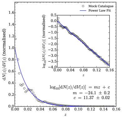
Figure 4: The volume-weighted redshift distribution the 6dFGS mock catalogue (open circles). The solid line shows the power fit to this distribution, which is provided to HADES as the estimate for the radial selection function of the mock catalogue. The inset panel shows the base-10 logarithm of the distribution. Stated in the plot are the values for the parameters, $m$ and $c$, for the power law fit.

As inputs, HADES requires only the galaxy positions, the sky completeness mask (in HEALPix format) and an estimate of the radial selection function of the mock catalogue. We calculate the radial selection function of the mock catalogue by computing the volume weighted redshift distribution, ${\rm d}N(z)/{\rm d}V(z)$, which we show in Fig. 4. Remarkably this function is very well described by a power-law, which is also shown. This power-law relation, re-normalised to the interval [0,1], is the selection function provided to HADES. HADES uses a convolution of the sky completeness mask and the radial selection function to construct a three-dimensional response operator, $R(\overrightarrow{x})$, which describes the completeness of the observations as a function of position, $\overrightarrow{x}$. For details on the data model and the implementation of the HADES algorithm we refer the interested reader to Jasche & Kitaura (2010); Jasche et al. (2010a) and Jasche & Wandelt (2012).

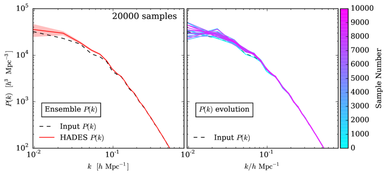
Figure 5: The matter power spectrum as recovered by HADES. The left-hand panel shows the ensemble mean power spectrum, obtained by averaging over 20,000 samples, with the shaded regions indicating the size of the standard deviation in each bin of wavenumber. The right-hand panel shows the evolution of the power spectrum with sample number for one HADES chain. The solid line for each estimate is coloured according to the number of the sample it was taken from. In each panel, the dashed line corresponds to the input power spectrum that HADES was provided with.

We infer the large-scale structure within a rectangular Cartesian domain of size length $981\,h^{-1}{\rm Mpc}\,\times\,955\,h^{-1}{\rm Mpc}\,\times\,511\,h^{-1}{\rm Mpc}$. This inference domain was chosen to optimally account for the geometry of the 6dFGS mock catalogue. The inference domain was subdivided into $256\,\times\,256\,\times\,128$ cells, allowing a grid resolution of $\sim 3.6\,h^{-1}{\rm Mpc}$. We note that the total number of inference parameters, which correspond to the density amplitudes in each of the grid cells, is $\sim 10^{6}$. This large number of parameters can be efficiently sampled by the HADES algorithm via a Hamiltonian Monte Carlo sampling framework. To explore the corresponding high dimensional parameter space we run four chains in parallel, each generating a total of $10,000$ data constrained realisations of the three-dimensional density field. Being a numerical representation of the full posterior distribution, this ensemble of density fields contains all of the information that could be extracted from observations and provides accurate quantification of uncertainties inherent to any cosmological observation.

3.2 Burn-in and statistical efficiency

As with any Markov Chain Monte-Carlo technique, there will be correlations between subsequent density field realisations generated by the Markov chain. For this reason the sampler requires a certain amount of sampling steps to decorrelate from the chosen initial conditions. This phase of a Markov sampler is referred to as the burn-in period. After this finite initial phase the Markov sampler generates density field realisations drawn from the correct target posterior distribution.

A simple monitor of burn-in is to follow the evolution of parameters with sample number (e.g. Eriksen et al., 2004; Jasche et al., 2010b). The right-hand panel of Fig. 5 shows the evolution of the recovered posterior matter power spectrum with sample number for the 10,000 samples in one of the four Markov chains. We can see that the chain has converged after approximately 2000 samples and starts exploring the parameters within the range of uncertainty. As a conservative measure, we discard the first 5000 samples in each chain to ensure that each chain has passed the initial burn-in phase. This leaves us with 5000 realisations of the density field for each chain, giving a total of 20,000 samples.

The left-hand panel of Fig. 5 shows the ensemble mean and variance on the power spectrum, obtained by averaging over the 20,000 converged samples. At small $k$ the power spectrum is biased high relative to the input power spectrum, likely due to the effect of galaxy bias. In its current form HADES assumes a constant linear bias. We assume an arbitrary bias value of 1.2, which, given the value of $\sigma_{8}$ used in the MS-W7 cosmology, is within $2\sigma$ of the bias estimates of Beutler et al. (2012). Another possible source of the excess power could be the appearance of repeated structures in the mock catalogue, arising due to our method of building the mock catalogue by replicating the simulation box.

3.3 Inferred density fields

We now examine the density field as inferred by HADES. In Fig. 6 we show slices, of approximately $4\,\,h^{-1}{\rm Mpc}$ thickness, through the HADES density field. The different columns correspond to a slice through each of the Cartesian axes. In the X and Y axes the slices are approximately at the origin, whilst the slice along the Z axis corresponds approximately to ${\rm Z}\sim-3\,\,h^{-1}{\rm Mpc}$. (This corresponds to the slice along the Z axis that is closest to the observer and whose volume is entirely spanned by the mock galaxy data). The top row shows slices through a single realisation of the recovered density field, whilst the middle row shows the same slices through the ensemble mean density field, $\langle\delta\rangle$, averaged over 20,000 samples. In the bottom row we show the ensemble variance of the recovered density field, $\sigma(\delta)$, again taken over 20,000 samples. From Fig. 6 we can see that for many regions in the inferred large-scale structure the ensemble variance is comparable to the ensemble mean, as expected for a Poisson process.

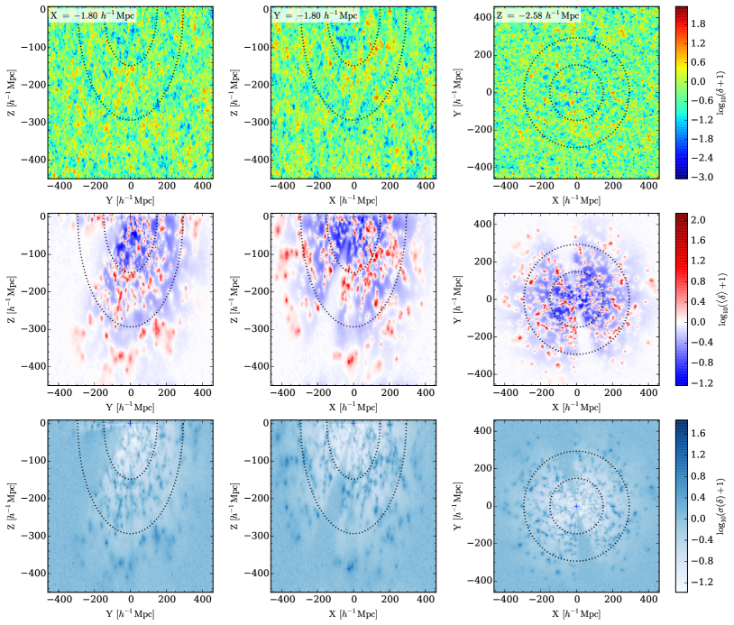
Figure 6: Slices showing the HADES density field in the three Cartesian axes. The resolution of the HADES reconstruction is approximately $4\,\,h^{-1}{\rm Mpc}$. The left-hand column shows a slice at $X\sim 0\,\,h^{-1}{\rm Mpc}$, the middle column shows a slice at $Y\sim 0\,\,h^{-1}{\rm Mpc}$ and the right-hand at $Z\sim-3\,\,h^{-1}{\rm Mpc}$. The top row shows a single realisation of the HADES density field. The middle row shows the ensemble average of the density field, obtained by averaging over 20,000 realisations. The bottom row shows the ensemble variance, again obtained by averaging over 20,000 realisations.

Comparing these results we can see that whilst the density field from individual samples appears very Gaussian, the ensemble mean density field is strikingly non-Gaussian, with the non-linear features of the cosmic web becoming clearly visible above the noise. High signal-to-noise structures, such as galaxy clusters and voids, are easily identifiable out to distances of approximately $200\,\,h^{-1}{\rm Mpc}$ from the observer, which for our cosmological model corresponds to a redshift of $z\sim 0.07$.

Note, however, that the masked regions, which are not constrained by observations and regions dominated by noise tend towards the mean density with $\langle\delta\rangle=0$. This behaviour is expected in regions without data constraints, where we expect to recover the cosmic mean density on average. One such example is the region of the mock survey masked by the galactic plane, which is not visible in individual realisations but becomes apparent in the ensemble properties. In each individual sample HADES is able to infer the large-scale structure in these regions, however the lack of constraints for these regions leads to a low signal-to-noise ratio for the inference in these regions so that over the ensemble 20,000 realisations the inferred density field averages out to the mean density.

3.4 Recovery of structures

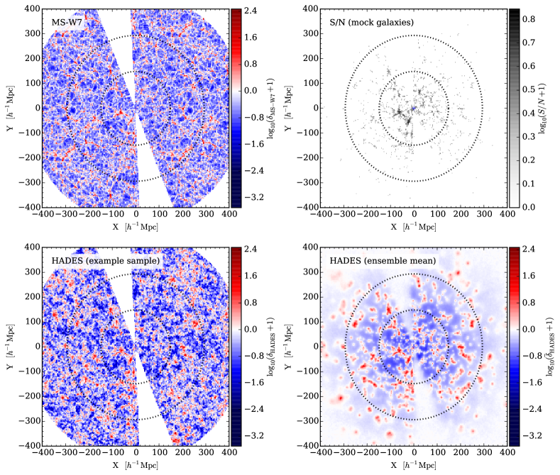
Figure 7: Zoomed slices through the HADES volume at ${\rm Z}\sim-3\,\,h^{-1}{\rm Mpc}$ showing the MS-W7 density field in the original mock catalogue (top left), the signal-to-noise (S/N) ratio of the mock observations (corresponding to the square root of the counts, top right), an example HADES realisation of the matter density field (bottom left) and the ensemble mean density field from HADES (bottom right). Note that in the left-hand panels, the density field is only shown for voxels where the response operator, $R$, is non-zero (i.e. where the completeness of the observations is non-zero). The dotted concentric circles correspond approximately to the median redshift and twice the median redshift of the mock galaxies.

Having seen that HADES is able to provide a realistic realisation for the cosmic web, we now consider the recovery of individual structures. We stress that the density field inferred by HADES corresponds to the continuous matter density field and that HADES does not provide any information for individual, discrete structures or for the halo density field. It does, however, provide insight into which individual structures, in particular clusters, could be identified as peaks in the inferred ensemble mean density field.

In Fig. 7 we compare an example density field realisation from HADES, as well as the ensemble density field, with the true density field for the mock catalogue, which corresponds to the density field from the $z=0$ snapshot of the MS-W7 simulation. We estimate the MS-W7 density field by replicating the MS-W7 box such that we can count the number of dark matter particles in each of the voxels in the HADES volume. Note that for the MS-W7 density field and the example HADES realisation, we only show the density field for voxels where the response operator, $R$, is non-zero (i.e. for voxels where the completeness of the observations is non-zero). Hence very distant regions, as well as regions behind the Galactic plane, are masked out. In addition, we also show in Fig. 7 the signal-to-noise ratio (S/N) for the observations, which we estimate as the square root of the galaxy counts in each HADES voxel.

A visual comparison of the MS-W7 density field with the HADES density fields, either the example realisation or the ensemble mean, shows that HADES is recovering the large-scale structure of the MS-W7 density field quite well, particularly for structures within twice the median redshift of the mock galaxies (as indicated by the outer of the two concentric circles). Individual structures in the MS-W7 density field can be identified in the HADES density fields. For example, the structure located near the observer at $(\mathrm{X},\mathrm{Y})\sim(-50,-20)\,h^{-1}{\rm Mpc}$, which is clearly visible in the galaxy counts, can be readily identified in both the HADES example realisation and the ensemble mean density field. Other structures further away from the observer, such as the filamentary structures at $(\mathrm{X},\mathrm{Y})\sim(-160,-140)\,h^{-1}{\rm Mpc}$ or $(\mathrm{X},\mathrm{Y})\sim(200,-40)\,h^{-1}{\rm Mpc}$, are not easily visible in the galaxy counts but are recovered by HADES, albeit at poorer resolution. At distances around twice the median redshift, or beyond, only a few individual clusters can be resolved, thanks to the counts of bright cluster galaxies. It is indeed noticeable that the fine filamentary structure in the MS-W7 density field is less well resolved by HADES compared to galaxy clusters, which constitute the nodes of the cosmic web. This, for example, could well be due to the fact that HADES is having to infer the density field using galaxies in redshift-space, which will lead to individual structures being smeared out by redshift-space distortion effects.

We note that for our analysis with HADES we have neglected the impact of uncertainties on the spectroscopic galaxy redshifts, which are not modelled in our mock catalogue. If we examine the redshift uncertainties, $\delta z$, of galaxies in the K-band selected sub-sample of the 6dFGS DR3, we find that the median fractional uncertainty is $\delta z/z=0.003^{+0.004}_{-0.001}$. (Uncertainties on the median value correspond to the difference between the median and the $\mathrm{10^{th}}$ and $\mathrm{90^{th}}$ percentiles). Assuming our given cosmology, we can convert this to a fractional uncertainty on the co-moving distance, $r$, of the galaxies, $\delta r/r$, where we take $\delta r=[r(z+\delta z)-r(z-\delta z)]/2$. This yields a typical fractional uncertainty of $\delta r/r=0.003^{+0.005}_{-0.001}$. For a galaxy at the median redshift of our mock survey, $z_{{\rm med}}\sim 0.05$, this corresponds to a typical uncertainty on the co-moving distance of approximately $\sim 0.45\,\,h^{-1}{\rm Mpc}$, which we note is much smaller than our grid resolution of $\sim 3.6\,\,h^{-1}{\rm Mpc}$ and so should have negligible impact on our results. If we apply our methodology to a catalogue of photometric redshifts, however, the impact from photometric redshift uncertainties would need to be considered.

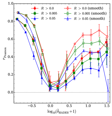
Figure 8: Pearson rank correlation coefficient indicating the mean strength of the correlation between the density field of the MS-W7 simulation and each of 20,000 HADES density field realisations. The correlation coefficient is shown as a function of density contrast from the ensemble mean of the HADES recovered density fields. The points show the mean coefficient for each density bin and the errorbars show one standard deviation. The filled symbols show the correlation obtained when considering only voxels for which the response operator, $R$, is greater than a threshold value: 0.0 (red circles), 0.005 (green squares) and 0.05 (blue triangles). The empty symbols show the correlation obtained when the density fields are first smoothed on scales of $\sim 18\,h^{-1}{\rm Mpc}$. (The resolution in the non-smoothed case is $\sim 3.6\,h^{-1}{\rm Mpc}$.)

To quantify our ability to recover of individual structures with HADES, we examine the correlation between the MS-W7 density field and the density field of the HADES realisations. To do this, we measure the Pearson correlation coefficient, which varies between $\pm 1$ and provides a measure of the linear correlation between two quantities, with $+1$ indicating a perfect positive correlation, $-1$ indicating a perfect negative correlation and $0$ indicating no correlation. We can therefore use the Pearson correlation coefficient to search for correlation between the true and inferred density fields. As such, we estimate the correlation between the MS-W7 density field and each of the individual 20,000 HADES realisations, i.e. giving us 20,000 estimates for the correlation. However, in each case instead of obtaining a single value for coefficient over the entire set of voxels, we split the voxels into density bins according to the density amplitude that that voxel has in the HADES ensemble mean density field. When measuring the coefficients we only consider voxels in the HADES volume where the response operator, $R$, is non-zero (as in the left-hand panels of Fig. 7).

In Fig. 8 we show the correlation coefficient as a function of the ensemble mean density from HADES. The filled circles show the mean correlation coefficient in each bin and the errorbars indicate one standard deviation. As can be seen, the correlation coefficient increases to larger positive values in the lowest and highest density bins, indicating that HADES is correctly identifying the most over-dense and under-dense voxels in the HADES grid, which correspond to the regions of highest signal-to-noise. The correlation is higher for the lowest density bins, which correspond to voids, than for the highest density bins, which correspond to clusters. This is likely due to voids having a larger volume filling factor than clusters and so being more easily identified in lower resolution reconstructions. In addition, due to their larger volume, the positions of the void centres will be less affected by redshift-space distortions than to the positions of clusters. As a consequence, large-scale structure inference algorithms have previously been used to identify and examine the properties of cosmic voids (e.g. Leclercq et al., 2015; Lavaux & Jasche, 2016). Towards the mean density, $\langle\delta\rangle\sim 0$, the correlation weakens significantly. This is understandable given that this density contrast will be associated with the regions of lowest signal-to-noise, such as the halos of small galaxy groups or even individual galaxies, where HADES is unable to make a decisive statement.

We show the correlation for two additional thresholds in the response operator: $R>0.005$ and $R>0.05$. These increasing limits of $R$ essentially limit us to smaller and smaller volumes about the observer: $R>0.005$ limits us to a spherical volume within approximately twice the median redshift and $R>0.05$ limits us to a spherical volume within approximately the median redshift (excluding, in all instances, the region behind the Galactic plane). Considering the highest density bins, the correlation decreases as the limit in $R$ is increased. Also, the uncertainty on the correlation also increases as we are restricted to a smaller volume. These results are consistent with the increasing impact of small-scale redshift-space distortions, which are more prominent closer to the observer and would shift the apparent positions of clusters in the HADES reconstructions, thus leading to a reduction in the correlation. Furthermore, we would expect the uncertainty to increase as we consider smaller volumes with a lower number statistics of clusters.

As a final demonstration, we also examine the impact on the correlation of smoothing the HADES and MS-W7 density fields. In Fig. 8 the empty points show the correlation coefficients obtained when the the HADES and MS-W7 density fields are first smoothed using a 3-dimensional Gaussian kernel, adopting a $5\times 5\times 5$ pixel window function. Given the pixel resolution, this window function has a scale of approximately $18\,h^{-1}{\rm Mpc}$. As such, this smoothing will remove all small-scale resolution but will allow us to consider whether the HADES and MS-W7 density fields correlate on large-scales. We see in Fig. 8 that smoothing the density fields in this way leads to an increase in the correlation in the majority of the highest density bins for each of the $R$ limits considered. Thus, we can conclude that the HADES density fields correlate well with density field from the MS-W7 on both small-scales ($\sim 4\,h^{-1}{\rm Mpc}$) and large-scales ($\sim 18\,h^{-1}{\rm Mpc}$). This result strongly supports the use of HADES density field realisations for identification of galaxy clusters (and voids) in galaxy survey datasets.

4 Bayesian Halo Detection

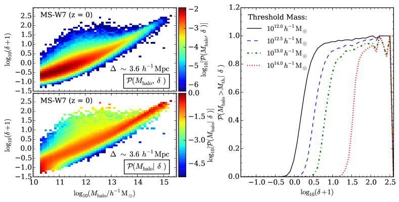
Figure 9: The upper left-hand panel shows the joint probability distribution $\mathcal{P}(M_{{\rm halo}},\delta)$ for the $z=0$ snapshot of the MS-W7 simulation, where $M_{{\rm halo}}$ is the mass of the most massive halo in any particular voxel. The lower left-hand panel shows the corresponding conditional probability distribution $\mathcal{P}(M_{{\rm halo}}|\delta)$, also for the $z=0$ snapshot of the MS-W7 simulation. This distribution shows the probability that, given the value for the density field, $\delta$, in a voxel, the most massive halo in that voxel has a mass $M_{\rm halo}$. The right-hand panel shows the probability $\mathcal{P}(M_{{\rm halo}}>M_{{\rm th.}}|\delta)$ that the most massive halo in a voxel has a mass greater than a threshold value, $M_{{\rm th}}$. Probability distributions are shown for four threshold masses: $10^{12.0}h^{-1}{\rm M_{\odot}}$ (black solid line), $10^{12.5}h^{-1}{\rm M_{\odot}}$ (blue dashed line), $10^{13.0}h^{-1}{\rm M_{\odot}}$ (green dot-dashed line) and $10^{14.0}h^{-1}{\rm M_{\odot}}$ (red dotted line).

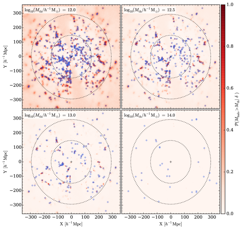
Figure 10: Slices through the HADES volume at ${\rm Z}\sim-3h^{-1}{\rm M_{\odot}}$ showing the detection probability for four different mass thresholds: $10^{12.0}h^{-1}{\rm M_{\odot}}$ (top left), $10^{12.5}h^{-1}{\rm M_{\odot}}$ (top right), $10^{13.0}h^{-1}{\rm M_{\odot}}$ (bottom left) and $10^{14.0}h^{-1}{\rm M_{\odot}}$ (bottom right). Open circles show the positions of the voxels for which the most massive halo has a mass above the corresponding threshold.

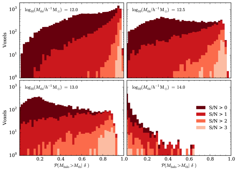
Figure 11: Distribution of detection probabilities for voxels whose most massive halo has a mass above $10^{12.0}h^{-1}{\rm M_{\odot}}$ (top left), $10^{12.5}h^{-1}{\rm M_{\odot}}$ (top right), $10^{13.0}h^{-1}{\rm M_{\odot}}$ (bottom left) and $10^{14.0}h^{-1}{\rm M_{\odot}}$ (bottom right). The different shaded histograms show the impact of placing an additional cut in S/N ratio and considering only those voxels above a specified threshold: $\mathrm{S/N}>\{0,1,2,3\}$.

Having determined that HADES is able to successfully identify the highest S/N peaks in the density field, we now present a Bayesian prescription that will allow us to extract information on the halo population from the inference results. In other words, given a set of observations, $d$, we wish to extract information on some specific quantity, $\alpha$.

4.1 Translating density to halo mass

In Bayesian parlance, we are interested in analysing the posterior distribution $\mathcal{P}(\alpha|d)$ and letting the data decide on the value of $\alpha$. In our approach we can formulate the posterior distribution $\mathcal{P}(\alpha|d)$ as a marginalisation over all density fields, at fixed redshift, as inferred within the HADES framework:

$$\qquad\qquad\quad\mathcal{P}(\alpha|d) = \int\mathrm{d}\delta\mathcal{P}(\delta,\alpha|d)$$ (4)

$$= \int\mathrm{d}\delta\mathcal{P}(\delta|d)\,\mathcal{P}(\alpha|\delta,d)$$

$$= \int\mathrm{d}\delta\mathcal{P}(\delta|d)\,\mathcal{P}(\alpha|\delta)$$

$$= \frac{1}{N_{\mathrm{samp}}}\sum_{i}\mathcal{P}(\alpha|\delta_{i}),$$

where we assume conditional independence $\mathcal{P}(\alpha|\delta,d)=\mathcal{P}(\alpha|\delta)$ once the true density field is given, and the posterior distribution $\mathcal{P}(\delta|d)=1/N_{\mathrm{samp}}\sum_{i}\delta^{D}(\delta-\delta_{i})$ is provided as an ensemble of data constrained density realisations via the HADES algorithm. The chain-rule approach described in Eq. (4) is frequently referred to as a Blackwell-Rao estimator. A similar approach has been implemented by Leclercq et al. (2015) to identify voids in the SDSS.

As demonstrated above, a full Bayesian quantification of unknown quantities $\alpha$ from the observations now reduces to providing the conditional probability distribution $\mathcal{P}(\alpha|\delta)$, which can be simply determined from numerical simulations of structure formation. Generally this approach can handle arbitrarily complex problems, requiring only a determination of the corresponding $\mathcal{P}(\alpha|\delta)$, which can be achieved via analytic or numerical means. For the sake of this work we will exemplify this approach to answer the question of how to find halos above a given mass in a galaxy survey such as the 6dFGS. Specifically, the question we wish to address is, for a voxel with a given density, $\delta$, what is the probability that the most massive dark matter halo found in that voxel has a mass, $M_{{\rm halo}}$, that is larger than a particular mass threshold, $M_{{\rm th.}}$. Given the approach of the Blackwell-Rao estimator, as described above, this task reduces to determining $\mathcal{P}(M_{{\rm halo}}>M_{{\rm th.}}|\delta)$, which describes the probability of finding the most massive halo of mass $M_{{\rm halo}}$ given a value of the density field $\delta$.

The first stage in determining $\mathcal{P}(M_{{\rm halo}}>M_{{\rm th.}}|\delta)$ is to consider a method for translating between density, $\delta$, and halo mass, $M_{{\rm halo}}$. This can be achieved by tabulating the conditional probability,

$$\mathcal{P}(M_{{\rm halo}}|\delta)=\frac{\mathcal{P}(M_{{\rm halo}},\delta)}{\mathcal{P}(\delta)},$$ (5)

from the snapshot of an N-body simulation. In practice, the joint probability, $\mathcal{P}(M_{{\rm halo}},\delta)$, can be calculated by simply building a two dimensional histogram between $\delta$ and $M_{{\rm halo}}$, where $M_{{\rm halo}}$ is the mass of the most massive halo in the voxel. The joint probability distribution is shown in the upper left-hand panel of Fig. 9. Here we estimate the conditional distribution $\mathcal{P}(M_{{\rm halo}}|\delta)$ using again the $z=0$ snapshot of the MS-W7. We estimate the density field for the simulation by binning the dark matter particles into a grid of $139^{3}$ voxels. Given the size of the simulation box, $500\,h^{-1}{\rm Mpc}$ on a side, this gives a resolution of $\sim 3.6\,h^{-1}{\rm Mpc}$, approximately identical to the resolution used in our HADES inference analysis. Note that we do not use the density field calculated according to the HADES volume as we do not want to bias the conditional probability by introducing repeated structures. The conditional probability distribution, shown in the lower left-hand panel of Fig. 9, is the conditional probability that the most massive halo in a $3.6\,\,h^{-1}{\rm Mpc}$ voxel with a given density, $\delta$, will have a mass of $M_{{\rm halo}}$. The distribution shows a clear, monotonic relation that we can use to translate between the density of a voxel and the mass of the most massive halo within that volume element. In reality the distribution $\mathcal{P}(M_{{\rm halo}}|\delta)$ will have an additional redshift dependence, which could be modelled by computing $\mathcal{P}(M_{{\rm halo}}|\delta)$ for each snapshot of the simulation and interpolating between the distributions. However, given that the 6dFGS is a very shallow survey, with median redshift $z_{\mathrm{med}}\sim 0.05$, for the purposes of demonstrating our methodology we can simply approximate the matter density field through the 6dFGS mock using the $z=0$ snapshot. We have examined the distribution $\mathcal{P}(M_{{\rm halo}}>M_{{\rm th.}}|\delta)$ from the MS-W7 snapshots for redshifts up to $z\sim 0.2$ (the approximate radial extent of the 6dFGS mock) and find negligible evolution of the distribution away from the $z=0$ distribution.

From $\mathcal{P}(M_{{\rm halo}}|\delta)$ we can make an estimate for $\mathcal{P}(M_{{\rm halo}}>M_{{\rm th}}|\delta)$ by marginalising over all halo masses above the threshold halo mass, $M_{{\rm th}}$. The right-hand panel of Fig. 9 shows estimates for $\mathcal{P}(M_{{\rm halo}}>M_{{\rm th.}}|\delta)$, at $z\sim 0$, for four different mass thresholds: $M_{{\rm th.}}=10^{12.0}h^{-1}{\rm M_{\odot}}$, $10^{12.5}h^{-1}{\rm M_{\odot}}$, $10^{13.0}h^{-1}{\rm M_{\odot}}$ and $10^{14.0}h^{-1}{\rm M_{\odot}}$. For each mass threshold, the detection probability for a halo undergoes quite a sharp transition as a function of density. Furthermore, the transition of the probability from zero to one occurs at higher densities for larger mass thresholds. We note that the detection probability drops back down to zero at $\log_{10}(\delta+1)\sim 2.5$ due to the limited volume of the MS-W7 simulation. However, for a larger volume simulation, above $\log_{10}(\delta+1)\sim 2.5$ the detection probability would remain constant at unity.

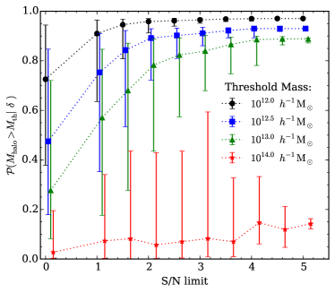
Figure 12: Change in detection probability as a function of signal-to-noise limit. The filled symbols show the median detection probability for those voxels that have a S/N above the corresponding limit and whose most massive halo has a mass above $10^{12.0}h^{-1}{\rm M_{\odot}}$ (circles), $10^{12.5}h^{-1}{\rm M_{\odot}}$ (squares), $10^{13.0}h^{-1}{\rm M_{\odot}}$ (triangles) and $10^{14.0}h^{-1}{\rm M_{\odot}}$ (stars). The error bars show the $\mathrm{10^{th}}$ and $\mathrm{90^{th}}$ percentiles.

4.2 Detection probability maps

Using this result we are therefore able to build maps of the detection probability for halos above specific threshold masses given some galaxy observation, $d$. These maps are built by using the Blackwell-Rao approach, as described in Eq. (4), and simply marginalising over all data constrained realisations of the density field obtained via the HADES, using the distributions in the right-hand panel of Fig. 9 to assign a weight to each voxel. In Fig. 10 we show maps for the halo detection probabilities for the four different mass thresholds: $\log_{10}(M_{{\rm th.}}/h^{-1}{\rm M_{\odot}})=\{12.0,12.5,13.0,14.0\}$. Given the mock catalogue and knowledge of the underlying halos, we can determine the mass of the most massive halo in each HADES voxel. (Note that this information is stored when we build the mock catalogue, before any geometrical, photometric or completeness limits are applied.) On top of the detection maps we indicate with blue circles those voxels whose most massive halo is above the specified threshold. We stress, however, that these detection maps are not only reconstructions of the halo distribution, but instead, for any position $\bar{x}$, quantify our belief that there exists a halo above a given mass threshold located at that point. This provides a natural quantification of detection uncertainties in the survey.

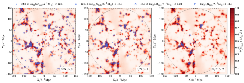
Figure 13: Three zoom in slices of the detection probability map for $M_{\mathrm{th}}=10^{12}h^{-1}{\rm M_{\odot}}$, showing the region within the median redshift of the mock catalogue (as indicated by the dotted circle). The blue circles show the positions of the voxels with a signal-to-noise ratio (S/N) above the specified threshold and whose most massive halo is within the particular mass bin. The S/N ratio thresholds are: $\mathrm{S/N}>0$ (left-hand panel), $\mathrm{S/N}>1$ (middle panel) and $\mathrm{S/N}>2$ (right-hand panel).

For the three lowest mass thresholds it can be seen that the detection probability for halos of respective masses is fairly high close to the observer where the survey generally exhibits high signal-to-noise ratios. As can be seen, many halos are correctly identified by the relative peaks in the detection probability. With increasing distance from the observer the detection of respective halo populations becomes increasingly uncertain. This is because, due to flux limitations of the survey, we only observe the brighter objects that are typically hosted by more massive halos at larger distances. Dim objects corresponding to less massive halos have a vanishing probability of being detected by the flux limited survey. As can be seen in Fig. 10, the respective panels correctly reflect this behaviour.

For the $M_{\mathrm{th.}}=10^{14}h^{-1}{\rm M_{\odot}}$ mass threshold, however, we see, on first inspection, very few detection peaks, with several halos appearing not to have a corresponding peak in the detection probability map. We see that, given our observational dataset, several of these mis-detections occur in noise-dominated regions, where we have only a handful of galaxies. If, however, we were to artificially boost the detection probabilities in the map, we would see that many of the halos do indeed correspond to relative peaks in the probability and that these peaks simply have a lower amplitude compared to the peaks in the detection maps for the other mass thresholds. This is due to our cosmological model and our prior belief of finding halos above a particular mass, which is encoded in the matter power spectrum. The $\mathrm{\Lambda}$CDM cosmological model predicts that in a given volume, such as that of the MS-W7 simulation, we should expect to find relatively few high density peaks compared to low density peaks and so would expect to find fewer high mass halos compared to lower mass halos. Suppose therefore we were to bet on finding a halo above $10^{14}h^{-1}{\rm M_{\odot}}$ at a particular position. Given our cosmological model, for noise-dominated regions we would be less confident and would not bet as highly on finding a halo above a higher mass threshold. As such, given the observational dataset, our halo detection methodology assigns a non-zero detection probability, but is conservative due to our physical expectation that we are generally less likely to find an extreme event. In a similar fashion, our methodology encodes the fact that we are more likely to detect a lower mass halo and so assigns a higher detection probability for lower mass thresholds.

There are several factors which could act to further smooth the amplitude of the detection probability peaks. Firstly the fact that we have fewer density high density peaks leads to the $\mathcal{P}(M_{{\rm halo}}|\delta)$ conditional probability, shown in the lower left-hand panel of Fig. 9, becoming noisier towards larger densities and halo masses. This increases the width of $\mathcal{P}(M_{{\rm halo}}|\delta)$, thus causing a particular density amplitude to correspond to a range of halo masses. As a result, more massive halos could potentially be mistaken for lower mass objects. Using a simulation with larger cosmological volume would help prevent this. Secondly, our modelling of phenomena such as galaxy bias could lead to a systematic offset between the density amplitudes in the simulation and the density amplitudes recovered by HADES. In this work we have assumed a fixed bias of $b=1.2$. The impact of galaxy bias could in future work be examined by reproducing the HADES inference analysis using a range of different bias values, though the ability of HADES to infer luminosity-dependent galaxy bias is also currently being tested. Finally, another important factor is redshift-space effects. The HADES reconstructions correspond to the redshift-space density field, whilst the calculated $\mathcal{P}(M_{{\rm halo}}|\delta)$ corresponds to the real-space density field of the N-body simulation. Redshift-space effects, such as fingers-of-god effects, act to smooth out real-space density peaks, especially density peaks. As such, this could again lead to a high mass halo being mistaken as a lower mass halo. The impact of redshift-space distortions in HADES is still being investigated (see Jasche & Wandelt, 2012) and will be considered in future work.

4.3 Recovery of individual clusters

To begin to quantify the success of the detection of halos we examine the distribution of probabilities for those voxels whose most massive halo is above the different mass thresholds. We plot these distributions, for each of the four mass thresholds, in Fig. 11. When considering all such voxels with a signal-to-noise ratio greater than zero, we see that, with the exception of the $10^{12}h^{-1}{\rm M_{\odot}}$ mass threshold, every distribution peaks at low probabilities. This is because, as discussed in the previous section, in noisier regions with lower signal-to-noise we have less confidence of detecting higher mass halos. We would therefore expect such voxels to be poorly constrained by HADES, leading to a reduced detection probability.

We show in Fig. 11, how the distribution of detection probabilities changes as we restrict ourselves to voxels with higher S/N ratios: $\mathrm{S/N}>1$, $\mathrm{S/N}>2$ and $\mathrm{S/N}>3$. As the S/N limit is increased the peak of the distribution shifts towards higher detection probabilities. In Fig. 12 we plot the change in the median detection probability as a function of S/N ratio. The increase in the median probability with increasing S/N ratio reflects our confidence in detecting a higher mass halo. For the highest mass threshold, $M_{\mathrm{th.}}=10^{14}h^{-1}{\rm M_{\odot}}$, we see a consistently low detection probability, as we have discussed previously. Note however that this mass threshold still displays a median probability that increases with increasing S/N, reflecting our increasing confidence of detecting a halo with mass above $10^{14}h^{-1}{\rm M_{\odot}}$ in highly constrained voxels.

As such, expressing the success of our detection methodology becomes a function of S/N. We demonstrate this visually in Fig. 13, where we zoom in on $M_{\mathrm{th.}}=10^{12}h^{-1}{\rm M_{\odot}}$ probability map for the region within the median redshift of the mock catalogue. In the three consecutive panels we overlay the positions of voxels with a S/N above a particular limiting value and where the most massive halo in that voxel is within a particular mass range. For the $\mathrm{S/N}>0$ panel we can see that there are several mis-detections, particularly for lower-mass halos. However, as we increase the S/N ratio we can see that the number of mis-detections decreases and the positions of the halos correlate well with large peaks in the detection probability.

Finally, we stress that this analysis serves as a proof of concept, where we have used a simple measurement task to demonstrate the feasibility of our Bayesian halo detection approach, as outlined above. However, the method only relies on the conditional distribution $\mathcal{P}(\alpha|\delta)$ of some quantity $\alpha$ given a density field $\delta$ (at a redshift $z$), which can either be generated via analytic calculations or extracted from simulations as described here. For this reason the proposed Bayesian detection methodology is a flexible and versatile approach that can be arbitrarily increased in complexity to test various quantities and features of the cosmic large-scale structure in cosmological datasets. The excellent agreement between the peaks in our detection probability maps and the positions of high S/N halos indicates that this methodology could be used in the construction of an accurate catalogue of probabilistic cluster candidates, though a resolution finer than $3.6\,h^{-1}{\rm Mpc}$ would likely be required.

5 Summary & Conclusions

We present a novel Bayesian methodology for inferring various properties of the cosmic large-scale structure. Specifically, we focus on determining the detection probability of halos with masses above different thresholds in cosmological observations, which may be subject to stochastic and systematic uncertainties. Our approach relies on the previously developed HADES algorithm, designed to infer the smooth matter density field of the cosmic large-scale structure in the non-linear regime, and the Blackwell-Rao Estimator, which we use to relate density field amplitudes to halo properties. In this work we present a proof-of-concept of our methodology by applying it to a realistic galaxy mock catalogue for which the halo positions and membership are already known.

We construct a realistic galaxy mock catalogue by populating the halos of a cosmological N-body simulation with galaxies from a semi-analytical galaxy formation model. The mock catalogue emulates the K-band selected catalogue of the 6dFGS final data release (DR3). We apply the HADES algorithm to the mock catalogue in four parallel Markov chains to generate a total of 20,000 realisations of the matter density field through approximately $0.5\,h^{-3}{\rm Gpc}^{3}$ of the volume of the mock catalogue, sampled at a resolution of approximately $3.6\,h^{-1}{\rm Mpc}$. Examination of recovery of the matter power spectrum suggests that the Markov chains converge within approximately 2000 samples. As a conservative measure, however, we remove the first 5000 samples from each chain to allow for burn-in, which leaves us with a total of 20,000 independent HADES realisations of the density field.

We present the ensemble mean and variance of the density field recovered by HADES. Despite the Gaussian nature of each individual sample, the ensemble mean density field is distinctly non-Gaussian, with large-scale structures such as galaxy clusters and voids, which constitute high signal-to-noise features, clearly identifiable out to twice the median redshift of the mock survey. To quantify the success of the recovery of structures by HADES we consider the correlation between the HADES density field and the MS-W7 density field, as estimated within the HADES volume. Examining the Pearson correlation as a function of HADES ensemble density we find a high correlation in the highest and lowest density bins. This result indicates that HADES is successfully recovering high signal-to-noise regions, such as clusters and voids.

Finally we present a Bayesian prescription to address the problem of extracting information for the halo population from a set of observations from a galaxy survey. Specifically, we use a Blackwell-Rao estimator to address the question, given a value for the density field, $\delta$, over a volume element at redshift, $z$, what is the probability, $\mathcal{P}(M_{{\rm halo}}>M_{{\rm th.}}|\delta)$, that the most massive halo within that volume has a mass, $M_{{\rm halo}}$, greater than some threshold value, $M_{{\rm th.}}$. A cosmological simulation can be used to construct the conditional probability $\mathcal{P}(M_{{\rm halo}}|\delta)$ for the mass of the most massive halo in a volume element. By marginalising over all HADES realisations and using the density amplitude to weight each voxel according to $\mathcal{P}(M_{{\rm halo}}>M_{{\rm th}}|\delta)$, we can construct maps of the detection probability for halos above selected threshold masses. For each mass threshold considered, the relative peaks in the detection probability correspond quite well to the positions of halos with masses above the threshold. However, for the highest mass threshold of $10^{14}h^{-1}{\rm M_{\odot}}$ the peaks in the detection probability have lower amplitude, which leads to an increasing number of apparent mis-detections. This is due to our cosmological model, which predicts that we should expect to find relatively few high mass halos compared to lower mass halos. As such, our methodology encodes this expectation and reflects our reduced confidence of detecting very massive halos, especially in regions of low signal-to-noise. This means, for example, that with increasing distance from the observer the probability of detection of more massive halo populations becomes increasingly uncertain. We find therefore that the success of the detection method is a function of the S/N ratio. For the three lowest mass thresholds, halos in voxels with $\mathrm{S/N}>1$ are typically detected with a probability greater than 0.5, whilst halos in voxels with $\mathrm{S/N}>2$ are typically detected with a probability in excess of 0.8.

Our Bayesian description provides a statistically thorough approach to quantify the detection probability and corresponding uncertainties for halos above a given mass threshold. Following this proof-of-concept we plan to, in future work, apply HADES and our halo detection prescription to the actual 6dFGS observational data. Beyond this our methodology can be applied to mock catalogues and actual observations of deeper spectroscopic surveys, in order to demonstrate the ability of our methodology to detect halos out at higher redshifts. We stress however that our methodology is versatile and can be applied to a wide variety of datasets, including deep catalogues of galaxies with photometric redshifts (thanks to the photometric redshift sampling that is possible with HADES). Therefore, we aim in future work to additionally apply the methodology to photometric datasets. As such, the Bayesian methodology that we have presented offers a promising approach for the analysis of ongoing and future large-scale structure surveys.

References

- Allen et al. (2011) Allen S. W., Evrard A. E., Mantz A. B., 2011, ARA&A, 49, 409
- Ascaso & Moles (2007) Ascaso B., Moles M., 2007, ApJ, 660, L89
- Ascaso et al. (2012) Ascaso B., Wittman D., Benítez N., 2012, MNRAS, 420, 1167
- Bartelmann & Schneider (2001) Bartelmann M., Schneider P., 2001, Phys. Rep., 340, 291
- Benitez et al. (2014) Benitez N., Dupke R., Moles M., Sodre L., Cenarro J., Marin-Franch A., Taylor K., Cristobal D. et al, 2014, arXiv:astro-ph/1403.5237
- Beutler et al. (2012) Beutler F., Blake C., Colless M., Jones D. H., Staveley-Smith L., Poole G. B., Campbell L., Parker Q. et al, 2012, MNRAS, 423, 3430
- Böhringer et al. (2004) Böhringer H., Schuecker P., Guzzo L., Collins C. A., Voges W., Cruddace R. G., Ortiz-Gil A., Chincarini G. et al, 2004, A&A, 425, 367
- Borgani & Guzzo (2001) Borgani S., Guzzo L., 2001, Nature, 409, 39
- Borgani et al. (2001) Borgani S., Rosati P., Tozzi P., Stanford S. A., Eisenhardt P. R., Lidman C., Holden B., Della Ceca R. et al, 2001, ApJ, 561, 13
- Botzler et al. (2004) Botzler C. S., Snigula J., Bender R., Hopp U., 2004, MNRAS, 349, 425
- Campbell et al. (2004) Campbell L., Saunders W., Colless M., 2004, MNRAS, 350, 1467
- Carlstrom et al. (2002) Carlstrom J. E., Holder G. P., Reese E. D., 2002, ARA&A, 40, 643
- Cole et al. (2000) Cole S., Lacey C. G., Baugh C. M., Frenk C. S., 2000, MNRAS, 319, 168
- Coles & Jones (1991) Coles P., Jones B., 1991, MNRAS, 248, 1
- Couch et al. (1991) Couch W. J., Ellis R. S., MacLaren I., Malin D. F., 1991, MNRAS, 249, 606
- Dalton et al. (1997) Dalton G. B., Maddox S. J., Sutherland W. J., Efstathiou G., 1997, MNRAS, 289, 263
- Davis et al. (1985) Davis M., Efstathiou G., Frenk C. S., White S. D. M., 1985, ApJ, 292, 371
- Driver et al. (2012) Driver S. P., Robotham A. S. G., Kelvin L., Alpaslan M., Baldry I. K., Bamford S. P., Brough S., Brown M. et al, 2012, MNRAS, 427, 3244
- Ebeling et al. (2000) Ebeling H., Edge A. C., Allen S. W., Crawford C. S., Fabian A. C., Huchra J. P., 2000, MNRAS, 318, 333
- Eke et al. (2004) Eke V. R., Baugh C. M., Cole S., Frenk C. S., Norberg P., Peacock J. A., Baldry I. K., Bland-Hawthorn J. et al, 2004, MNRAS, 348, 866
- Erdoǧdu et al. (2004) Erdoǧdu P., Lahav O., Zaroubi S., Efstathiou G., Moody S., Peacock J. A., Colless M., Baldry I. K. et al, 2004, MNRAS, 352, 939
- Eriksen et al. (2004) Eriksen H. K., O’Dwyer I. J., Jewell J. B., Wandelt B. D., Larson D. L., Górski K. M., Levin S., Banday A. J. et al, 2004, ApJS, 155, 227
- Farrens et al. (2011) Farrens S., Abdalla F. B., Cypriano E. S., Sabiu C., Blake C., 2011, MNRAS, 417, 1402
- Fisher et al. (1994) Fisher K. B., Scharf C. A., Lahav O., 1994, MNRAS, 266, 219
- Gladders & Yee (2000) Gladders M. D., Yee H. K. C., 2000, AJ, 120, 2148
- Gladders & Yee (2005) —, 2005, ApJS, 157, 1
- Gonzalez-Perez et al. (2014) Gonzalez-Perez V., Lacey C. G., Baugh C. M., Lagos C. D. P., Helly J., Campbell D. J. R., Mitchell P. D., 2014, MNRAS, 439, 264
- Górski et al. (2005) Górski K. M., Hivon E., Banday A. J., Wandelt B. D., Hansen F. K., Reinecke M., Bartelmann M., 2005, ApJ, 622, 759
- Goto et al. (2002) Goto T., Sekiguchi M., Nichol R. C., Bahcall N. A., Kim R. S. J., Annis J., Ivezić Ž., Brinkmann J. et al, 2002, AJ, 123, 1807
- Guo et al. (2013) Guo Q., White S., Angulo R. E., Henriques B., Lemson G., Boylan-Kolchin M., Thomas P., Short C., 2013, MNRAS, 428, 1351
- Hansen et al. (2005) Hansen S. M., McKay T. A., Wechsler R. H., Annis J., Sheldon E. S., Kimball A., 2005, ApJ, 633, 122
- Huchra & Geller (1982) Huchra J. P., Geller M. J., 1982, ApJ, 257, 423
- Ivezic et al. (2008) Ivezic Z., Axelrod T., Brandt W. N., Burke D. L., Claver C. F., Connolly A., Cook K. H., Gee P. et al, 2008, Serbian Astronomical Journal, 176, 1
- Jasche & Kitaura (2010) Jasche J., Kitaura F. S., 2010, MNRAS, 407, 29
- Jasche et al. (2010a) Jasche J., Kitaura F. S., Li C., Enßlin T. A., 2010a, MNRAS, 409, 355
- Jasche et al. (2010b) Jasche J., Kitaura F. S., Wandelt B. D., Enßlin T. A., 2010b, MNRAS, 406, 60
- Jasche & Lavaux (2015) Jasche J., Lavaux G., 2015, MNRAS, 447, 1204
- Jasche & Wandelt (2012) Jasche J., Wandelt B. D., 2012, MNRAS, 425, 1042
- Jasche & Wandelt (2013a) —, 2013a, MNRAS, 432, 894
- Jasche & Wandelt (2013b) —, 2013b, ApJ, 779, 15
- Jian et al. (2014) Jian H.-Y., Lin L., Chiueh T., Lin K.-Y., Liu H. B., Merson A., Baugh C., Huang J.-S. et al, 2014, ApJ, 788, 109
- Jiang et al. (2014) Jiang L., Helly J. C., Cole S., Frenk C. S., 2014, MNRAS, 440, 2115
- Jones et al. (2006) Jones D. H., Peterson B. A., Colless M., Saunders W., 2006, MNRAS, 369, 25
- Jones et al. (2009) Jones D. H., Read M. A., Saunders W., Colless M., Jarrett T., Parker Q. A., Fairall A. P., Mauch T. et al, 2009, MNRAS, 399, 683
- Jones et al. (2004) Jones D. H., Saunders W., Colless M., Read M. A., Parker Q. A., Watson F. G., Campbell L. A., Burkey D. et al, 2004, MNRAS, 355, 747
- Kayo et al. (2001) Kayo I., Taruya A., Suto Y., 2001, ApJ, 561, 22
- Kepner et al. (1999) Kepner J., Fan X., Bahcall N., Gunn J., Lupton R., Xu G., 1999, ApJ, 517, 78
- Kim et al. (2002) Kim R. S. J., Kepner J. V., Postman M., Strauss M. A., Bahcall N. A., Gunn J. E., Lupton R. H., Annis J. et al, 2002, AJ, 123, 20
- Kitaura et al. (2009) Kitaura F. S., Jasche J., Li C., Enßlin T. A., Metcalf R. B., Wandelt B. D., Lemson G., White S. D. M., 2009, MNRAS, 400, 183
- Kochanek et al. (2001) Kochanek C. S., Pahre M. A., Falco E. E., Huchra J. P., Mader J., Jarrett T. H., Chester T., Cutri R. et al, 2001, ApJ, 560, 566
- Koester et al. (2007) Koester B. P., McKay T. A., Annis J., Wechsler R. H., Evrard A. E., Rozo E., Bleem L., Sheldon E. S. et al, 2007, ApJ, 660, 221
- Komatsu et al. (2011) Komatsu E., Smith K. M., Dunkley J., Bennett C. L., Gold B., Hinshaw G., Jarosik N., Larson D. et al, 2011, ApJS, 192, 18
- Kravtsov & Borgani (2012) Kravtsov A. V., Borgani S., 2012, ARA&A, 50, 353
- Laureijs et al. (2011) Laureijs R., Amiaux J., Arduini S., Auguères J. ., Brinchmann J., Cole R., Cropper M., Dabin C. et al, 2011, arXiv:astro-ph/1110.3193
- Lavaux & Jasche (2016) Lavaux G., Jasche J., 2016, MNRAS, 455, 3169
- Layzer (1956) Layzer D., 1956, AJ, 61, 383
- Leclercq et al. (2015) Leclercq F., Jasche J., Sutter P. M., Hamaus N., Wandelt B., 2015, J. Cosmology Astropart. Phys, 3, 047
- Leonard et al. (2014) Leonard A., Lanusse F., Starck J.-L., 2014, MNRAS, 440, 1281
- Lidman & Peterson (1996) Lidman C. E., Peterson B. A., 1996, AJ, 112, 2454
- López-Cruz et al. (2004) López-Cruz O., Barkhouse W. A., Yee H. K. C., 2004, ApJ, 614, 679
- Marinoni et al. (2002) Marinoni C., Davis M., Newman J. A., Coil A. L., 2002, ApJ, 580, 122
- Martínez & Saar (2002) Martínez V. J., Saar E., 2002, Statistics of the Galaxy Distribution. Chapman &
- Merloni et al. (2012) Merloni A., Predehl P., Becker W., Böhringer H., Boller T., Brunner H., Brusa M., Dennerl K. et al, 2012, arXiv:astro-ph/1209.3114
- Merson et al. (2013) Merson A. I., Baugh C. M., Helly J. C., Gonzalez-Perez V., Cole S., Bielby R., Norberg P., Frenk C. S. et al, 2013, MNRAS, 429, 556
- Milkeraitis et al. (2010) Milkeraitis M., van Waerbeke L., Heymans C., Hildebrandt H., Dietrich J. P., Erben T., 2010, MNRAS, 406, 673
- Miller et al. (2005) Miller C. J., Nichol R. C., Reichart D., Wechsler R. H., Evrard A. E., Annis J., McKay T. A., Bahcall N. A. et al, 2005, AJ, 130, 968
- Murphy et al. (2012) Murphy D. N. A., Geach J. E., Bower R. G., 2012, MNRAS, 420, 1861
- Parker et al. (1998) Parker Q. A., Watson F. G., Miziarski S., 1998, in Astronomical Society of the Pacific Conference Series, Vol. 152, Fiber Optics in Astronomy III, Arribas S., Mediavilla E., Watson F., eds., p. 80
- Peebles (1980) Peebles P. J. E., 1980, The large-scale structure of the universe
- Poggianti (1997) Poggianti B. M., 1997, A&AS, 122
- Postman et al. (1996) Postman M., Lubin L. M., Gunn J. E., Oke J. B., Hoessel J. G., Schneider D. P., Christensen J. A., 1996, AJ, 111, 615
- Ramella et al. (2001) Ramella M., Boschin W., Fadda D., Nonino M., 2001, A&A, 368, 776
- Ramella et al. (2002) Ramella M., Geller M. J., Pisani A., da Costa L. N., 2002, AJ, 123, 2976
- Robotham et al. (2011) Robotham A. S. G., Norberg P., Driver S. P., Baldry I. K., Bamford S. P., Hopkins A. M., Liske J., Loveday J. et al, 2011, MNRAS, 416, 2640
- Rosati et al. (2002) Rosati P., Borgani S., Norman C., 2002, ARA&A, 40, 539
- Rykoff et al. (2014) Rykoff E. S., Rozo E., Busha M. T., Cunha C. E., Finoguenov A., Evrard A., Hao J., Koester B. P. et al, 2014, ApJ, 785, 104
- Schechter (1976) Schechter P., 1976, ApJ, 203, 297
- Springel et al. (2005) Springel V., White S. D. M., Jenkins A., Frenk C. S., Yoshida N., Gao L., Navarro J., Thacker R. et al, 2005, Nature, 435, 629
- Springel et al. (2001) Springel V., White S. D. M., Tormen G., Kauffmann G., 2001, MNRAS, 328, 726
- Stanford et al. (1998) Stanford S. A., Eisenhardt P. R., Dickinson M., 1998, ApJ, 492, 461
- Sunyaev & Zeldovich (1972) Sunyaev R. A., Zeldovich Y. B., 1972, Comments on Astrophysics and Space Physics, 4, 173
- The Dark Energy Survey Collaboration (2005) The Dark Energy Survey Collaboration, 2005, arXiv:astro-ph/0510346
- Tyson et al. (1990) Tyson J. A., Valdes F., Wenk R. A., 1990, ApJ, 349, L1
- Voit (2005) Voit G. M., 2005, Reviews of Modern Physics, 77, 207
- Watson et al. (2000) Watson F. G., Parker Q. A., Bogatu G., Farrell T. J., Hingley B. E., Miziarski S., 2000, in Society of Photo-Optical Instrumentation Engineers (SPIE) Conference Series, Vol. 4008, Optical and IR Telescope Instrumentation and Detectors, Iye M., Moorwood A. F., eds., pp. 123–128
- York et al. (2000) York D. G., Adelman J., Anderson Jr. J. E., Anderson S. F., Annis J., Bahcall N. A., Bakken J. A., Barkhouser R. et al, 2000, AJ, 120, 1579
- Zaroubi et al. (1995) Zaroubi S., Hoffman Y., Fisher K. B., Lahav O., 1995, ApJ, 449, 446