ALMA Census of Faint 1.2 mm Sources Down to 0.02 mJy:
Extragalactic Background Light and Dust-Poor High-$z$ Galaxies

Abstract

We present statistics of 133 faint 1.2-mm continuum sources detected in about 120 deep ALMA pointing data that include all the archival deep data available by 2015 June. We derive number counts of 1.2 mm continuum sources down to 0.02 mJy partly with the assistance of gravitational lensing, and find that the total integrated 1.2 mm flux of the securely identified sources is 22.9${}^{+6.7}_{-5.6}$ Jy deg^-2 that corresponds to 104${}^{+31}_{-25}$% of the extragalactic background light (EBL) measured by COBE observations. These results suggest that the major 1.2 mm EBL contributors are sources with 0.02 mJy, and that very faint 1.2 mm sources with $\lesssim$0.02 mJy contribute negligibly to the EBL with the possible flattening and/or truncation of number counts in this very faint flux regime. To understand the physical origin of our faint ALMA sources, we measure the galaxy bias $b_{g}$ by the counts-in-cells technique, and place a stringent upper limit of $b_{g}<3.5$ that is not similar to $b_{g}$ values of massive DRGs and SMGs but comparable to those of UV-bright sBzKs and LBGs. Moreover, in optical and near-infrared (NIR) deep fields, we identify optical-NIR counterparts for 59% of our faint ALMA sources, majority of which have luminosities, colors, and the IRX-$\beta$ relation same as sBzKs and LBGs. We thus conclude that about a half of our faint ALMA sources are dust-poor high-$z$ galaxies as known as sBzKs and LBGs in optical studies, and that these faint ALMA sources are not miniature (U)LIRGs simply scaled down with the infrared brightness.

1. Introduction

Since the infrared (IR) extragalactic background light (EBL) was first identified by the Cosmic Background Explorer (COBE) satellite, it has been known that the total energy of IR EBL is comparable to that of the optical EBL (puget1996; fixsen1998; hauser1998; hauser2001; dole2006). Because dusty star-forming galaxies at high redshift should significantly contribute to the IR EBL, the IR EBL is key to understanding the dusty-side of the cosmic star formation history and to constraining physical parameters of galaxy formation models (e.g., granato2004; baugh2005; fontanot2007; shimizu2012; hayward2013).

To reveal the origin of the IR EBL, we need reliable number counts from bright to faint flux limits. The IR EBL of the low-frequency end, at submillimeter (submm) and millimeter (mm) wavelengths, is one of the most advantageous wavelength regimes, due to the negative k-correction. Previous blank field observations with single dish telescopes have revealed that the bright dusty high-$z$ objects of submillimeter galaxies (SMGs; lagache2005) are not major contributors of the EBL. SCUBA and LABOCA observations have resolved $20-40\%$ of the EBL at submm wavelength (e.g., eales2000; smail2002; coppin2006; knudsen2008; weiss2009). Similar results have been obtained by AzTEC observations that they have resolved $10-20\%$ of the EBL at mm wavelength (e.g., perera2008; hatsukade2011; scott2012). These observations suggest that there should exist high-$z$ populations different from SMGs, and that such populations are major EBL contributors in submm and mm wavelengths.

There are two observational challenges for fully resolving the EBL. First is the spatial resolution. The poor spatial resolution of the single-dish observations causes the serious source confusion (condon1974) that skews the observed number counts. Second is the sensitivity. Most of the submm and mm telescopes reach the limiting fluxes of $\sim 1$ mJy that correspond to the flux range of the SMGs. To detect submm sources fainter than $\sim 1$ mJy, there are many efforts (e.g., smail2002; chapman2002; knudsen2008; johansson2011; chen2013). knudsen2008 and chen2013 observe massive galaxy clusters at $850\ \mu$m for gravitationally lensed sources, and resolved 50%$-$180% of the EBL down to the intrinsic flux of $S_{\rm 850\ \mu m}>0.1$ mJy. These results indicate that there exist faint ($<1$ mJy) populations significantly contributing to the EBL (e.g., smail2002; knudsen2008). However, large uncertainties of the measurements still remain, due to the source blending and cosmic variance. Moreover, the physical origin of these faint submm and mm sources is unknown.

The Atacama Large Millimeter $/$ submillimeter Array (ALMA) enables us to investigate the faint submm and mm sources with the negligibly small uncertainties of the source confusion and blending, having its capabilities of high angular resolution and sensitivity. The first ALMA mm search for faint sources below $S_{\rm 1mm}\sim 1.0$ mJy with no lensing effect has been conducted by hatsukade2013. The study reports that they resolve $\sim$80% of the EBL down to $S_{\rm 1mm}=0.1$ mJy in 20 targets residing in one blank field of the Subaru$/$XMM-Newton Deep Survey (SXDS; furusawa2008). Due to the single field observations, this result would include unknown effects of cosmic variance. Subsequently, using multi-field deep ALMA $1$mm maps of Bands 6 and 7 down to the flux limit of $S_{\rm 1mm}=0.1$ mJy, ono2014 and carniani2015 have claimed an EBL resolved fraction of $\sim$60% that is smaller than the one of hatsukade2013. The uncertainties from cosmic variance are probably reduced with the multi-field data. Including the effects of the cosmic variance, only about a half of the EBL has been resolved with the present ALMA flux limit of $S_{\rm 1mm}=0.1$ mJy.

There is another remaining issue about the IR EBL. Although these studies newly identify faint ALMA sources ($S_{\rm 1mm}<1.0$ mJy) contributing to the half of the IR EBL, these studies do not clearly answer to the question about the connection between the faint ALMA sources and optically selected high-$z$ galaxies. Recent observations with Herschel have revealed that typical UV-selected galaxies such as Lyman-break galaxies (LBGs) have a median total (8-1000 $\mu$m) luminosity of $L_{\rm IR}\simeq 2.2\times 10^{11}L_{\odot}$ (reddy2012; lee2012; davies2013). The stacking analysis of Herschel and ALMA data has also shown that $K$-selected galaxies, including star-forming BzK galaxies (sBzKs), have total IR luminosities of $L_{\rm IR}=(5-11)\times 10^{11}L_{\odot}$ (decarli2014). These ranges of the IR luminosities of LBGs and sBzKs correspond to the mm flux of $S_{\rm 1mm}\sim 0.1-1$ mJy if we assume a modified black body with $\beta_{\rm d}=1.8$, dust temperature $T_{\rm d}=35$K, and a source redshift $z=2.5$. This mm flux range is similar to the one of the faint ALMA sources, implying that these sources could be mm counterparts of the optically selected galaxies.

There is another approach for characterizing the faint ALMA sources. Because the spatial distribution of galaxies is related to the underlying distribution of dark haloes in the standard scenario of structure formation in $\Lambda$CDM universe, the clustering analysis is a powerful tool for understanding the connection between various galaxy populations. Clustering analyses have been carried out over the past decade for bright SMGs observed with single-dish telescopes, and concluded that the clustering amplitudes, or galaxy biases, are large, and that the hosting dark halo masses of the bright SMGs are estimated to be $\sim 10^{13}M_{\odot}$ (webb2003; blain2004; weiss2009; williams2011; hickox2012, cf. miller2015). On the other hand, however, the dark halo properties of the faint ALMA sources are poorly known, except for the result of ono2014 who have obtained, for the first time, a meaningful constraint on a galaxy bias, $b_{\rm g}\leq 4$, for faint ALMA sources. In this way, the faint ALMA sources are not well studied. To understand the physical origin of faint ALMA sources, one should study faint ALMA sources with a more complete data set on the basis of individual sources as well as statistics.

In this paper, we analyze the large dataset of multi-field deep ALMA data including the complete deep datasets archived by 2015 June. Sixty-six independent-field and one cluster maps are taken by $\sim 120$ ALMA pointings in Band 6$/$7 to reveal the origins of the EBL and faint ALMA sources in mm wavelength. Note that this is the first step for statistically investigating faint sources behind a lensing cluster with ALMA. The structure of this paper is as follows. In Section 2, we describe the observations and the data reduction. Section 3 outlines the method of the source extraction, our simulations for deriving the number counts, and the mass model development for the cluster. We compare the number counts from our and previous studies, and estimate the resolved fraction of the EBL at 1.2 mm in section 4. In Section 5, we report the results of the clustering analysis for our faint ALMA sources. We investigate optical-NIR counterparts of our faint ALMA sources in Section 6. The summary of this study is presented in Section LABEL:sec:summary.

Throughout this paper, we assume a flat universe with $\Omega_{\rm m}=0.3$, $\Omega_{\Lambda}=0.7$, $\sigma_{8}=0.8$, and $H_{0}=70$ km s^-1 Mpc^-1. We use magnitudes in the AB system (Oke & Gunn 1983).

2. Data and Reduction

We use 67 continuum maps obtained by $\sim 120$ pointing of the ALMA cycle 0-2 observations in Band 6$/$7 that accomplish high sensitivities and angular resolutions. Tables 1 and 2 present the summary and the detailed properties, respectively, for these 67 continuum maps. We define sub-datasets by the mapping modes and the depths because these two conditions would make different systematics. For the mapping mode definitions, there are maps targeting field regions by single pointing observations, referred to as ’field’ data, 4 and 62 out of which are taken from our programs and the ALMA archive, respectively. One map for a galaxy cluster taken by mapping observations, referred to as ’cluster’ data, is from the ALMA archive.

For the depth definitions, we divide these 66 maps of ’field’ data into two sub-datasets with low ($\leq 60\ \mu$Jy) and high ($>60\ \mu$Jy) noise levels, which we refer to as ’deep’ and ’medium-deep’ data, respectively. This is because the short-integration data would have more chances to contain systematic noise. As shown in Table 2, we use the sub-dataset names of A and B for the deep and medium-deep field data, respectively. The sub-dataset name of the deep cluster data is C.

In this section, we describe the details of these 67 continuum maps of ’deep’, ’medium-deep’, and ’cluster’ data, and present our reduction procedures.

Table 1Data Summary

Sub-Dataset	Number of Maps
(1)	(2)
Deep data (A)	41
Medium-deep data (B)	25
Cluster data (C)	1

Note. — The sub-dataset names of A, B, and C are written in parenthesis. (1): ALMA maps with low ($\leq 60\ \mu$Jy) and high ($>60\ \mu$Jy) noise levels are referred to as Deep and Medium-deep data, respectively. (2): Number of the ALMA maps in each sub-dataset.

Table 2 ALMA Maps of this Study

Map ID	Target	$\lambda_{\rm obs}$	$\nu_{\rm obs}$ (Band)	$\sigma_{\rm cont}$	beam size	$S_{1.2{\rm mm}}/S_{\rm obs}$	Ref.	Project ID
		(mm)	(GHz)	($\mu$Jy beam-1)	(${}^{\prime\prime}\times^{\prime\prime}$)
		(1)	(2)	(3)	(4)	(5)	(6)
	Deep Data (A)
1	BDF-3299	1.30	227 (6)	8.5	0.79$\times$0.58	1.28	(a),(b)	2012.A.00040.S
								2012.1.00719.S
2	GRB090423	1.35	222 (6)	10.3	0.98$\times$0.75	1.45	(c),(d)	2012.1.00953.S
3	NB101-S-2904	1.26	238 (6)	11.4	0.43$\times$0.33	1.16	(e)	2012.1.00088.S
4	NB816-S-61269	1.03	291 (7)	13.0	0.45$\times$0.42	0.63	(f)	2012.1.00602.S
5	rxj0806	1.31	229 (6)	16.6	0.78$\times$0.63	1.31	(g)	2012.1.00610.S
6	Himiko	1.16	259 (6)	17.0	0.81$\times$0.56	0.90	(h),(i)	2011.0.00115.S
7	BDF-521	1.30	230 (6)	17.7	0.68$\times$0.51	1.28	(a),(b)	2012.1.00719.S
8	IOK-1	1.29	232 (6)	18.8	1.08$\times$0.78	1.25	(j),(k)	2011.0.00767.S
9	rxj2143	1.26	238 (6)	20.8	0.60$\times$0.43	1.16	(l)	2012.1.00610.S
10	CFHQSJ2329-0301	1.20	250 (6)	21.0	0.73$\times$0.63	1.00	(m),(n)	2011.0.00243.S
11	SDF-46975	1.22	244 (6)	21.2	1.23$\times$0.98	1.05	(o),(b)	2012.1.00719.S
12	ID239	1.29	232 (6)	21.7	1.88$\times$0.90	1.25	$\cdots$	2012.1.00076.S
13	GRB020819B	1.18	254 (6)	22.6	0.91$\times$0.72	0.95	(p)	2011.0.00232.S
14	CFHQSJ0055+0146	1.09	273 (6)	23.3	0.69$\times$0.55	0.75	(m)	2012.1.00676.S
15	ID182	1.23	244 (6)	23.8	1.33$\times$0.89	1.08	$\cdots$	2012.1.00076.S
16	ID220	1.23	244 (6)	24.2	1.33$\times$0.88	1.08	$\cdots$	2012.1.00076.S
17	ID244	1.29	232 (6)	24.1	1.87$\times$0.90	1.25	$\cdots$	2012.1.00076.S
18	CFHQSJ2229+1457	1.12	266 (6)	24.9	0.79$\times$0.70	0.81	(m)	2012.1.00676.S
19	ID247	1.29	232 (6)	25.1	1.87$\times$0.90	1.25	$\cdots$	2012.1.00076.S
20	ID209	1.29	232 (6)	25.8	1.23$\times$1.01	1.25	$\cdots$	2012.1.00076.S
21	CFHQSJ0210-0456	1.20	249 (6)	27.2	0.92$\times$0.61	1.00	(m),(n)	2011.0.00243.S
22	MSDM80+3	1.06	283 (7)	28.4	0.84$\times$0.63	0.69	(q)	2012.1.00536.S
23	GRB051022	1.15	262 (6)	28.6	1.15$\times$0.77	0.88	(p)	2011.0.00232.S
24	ID217	1.23	244 (6)	30.3	1.33$\times$0.93	1.08	$\cdots$	2012.1.00076.S
25	ID225	1.23	244 (6)	31.6	1.34$\times$0.93	1.08	$\cdots$	2012.1.00076.S
26	SXDS19723	1.27	236 (6)	38.5	0.83$\times$0.68	1.19	(r),(s)	2011.0.00648.S
27	SXDS28019	1.27	236 (6)	38.9	0.84$\times$0.68	1.19	(r),(s)	2011.0.00648.S
28	SXDS22198	1.27	236 (6)	39.0	0.86$\times$0.68	1.19	(r),(s)	2011.0.00648.S
29	SXDS35572	1.27	236 (6)	39.3	0.84$\times$0.68	1.19	(r),(s)	2011.0.00648.S
30	SXDS103139	1.27	236 (6)	39.7	0.83$\times$0.68	1.19	(r),(s)	2011.0.00648.S
31	NB921-N-79144	1.22	245 (6)	50.1	0.76$\times$0.63	1.05	(h),(f)	2012.1.00602.S
32	SXDS42087	1.30	231 (6)	52.9	0.80$\times$0.66	1.28	(r),(s)	2011.0.00648.S
33	SXDS79307	1.30	231 (6)	53.7	0.80$\times$0.66	1.28	(r),(s)	2011.0.00648.S
34	SXDS31189	1.30	231 (6)	54.4	0.81$\times$0.66	1.28	(r),(s)	2011.0.00648.S
35	MSDM29.5-5	1.06	283 (7)	54.6	0.71$\times$0.53	0.69	(q)	2012.1.00536.S
36	HiZELS-UDS-NBK-8806	1.39	216 (6)	55.0	1.86$\times$0.89	1.58	$\cdots$	2012.1.00934.S
37	HiZELS-UDS-NBK-11473	1.39	216 (6)	55.3	1.86$\times$0.89	1.58	$\cdots$	2012.1.00934.S
38	MSDM71-5	1.06	283 (7)	56.1	0.72$\times$0.53	0.69	(q)	2012.1.00536.S
39	HiZELS-UDS-NBK-13486	1.39	216 (6)	56.4	1.86$\times$0.89	1.58	$\cdots$	2012.1.00934.S
40	HiZELS-UDS-NBK-11961	1.39	216 (6)	58.3	1.86$\times$0.89	1.58	$\cdots$	2012.1.00934.S
41	ID125	1.09	273 (6)	59.1	1.30$\times$0.73	0.75	$\cdots$	2012.1.00076.S
	Medium-Deep Data (B)
42	ID098	1.09	273 (6)	60.1	1.30$\times$0.72	0.75	$\cdots$	2012.1.00076.S
43	ID093	1.09	273 (6)	60.3	1.30$\times$0.72	0.75	$\cdots$	2012.1.00076.S
44	ID143	1.09	273 (6)	61.7	1.31$\times$0.72	0.75	$\cdots$	2012.1.00076.S
45	SXDS33244	1.25	240 (6)	67.5	1.04$\times$0.64	1.13	(r),(s)	2011.0.00648.S
46	ID163	1.19	252 (6)	68.2	1.36$\times$0.92	0.97	$\cdots$	2012.1.00076.S
47	ID204	1.19	252 (6)	69.2	1.24$\times$0.86	0.97	$\cdots$	2012.1.00076.S
48	SXDS13316	1.23	244 (6)	69.3	0.87$\times$0.64	1.08	(r),(s)	2011.0.00648.S
49	ID158	1.19	252 (6)	69.5	1.35$\times$0.92	0.97	$\cdots$	2012.1.00076.S
50	ID192	1.19	252 (6)	69.7	1.24$\times$0.86	0.97	$\cdots$	2012.1.00076.S
51	SXDS59863	1.23	244 (6)	71.6	0.85$\times$0.65	1.08	(r),(s)	2011.0.00648.S
52	ID177	1.13	264 (6)	73.0	1.24$\times$0.86	0.83	$\cdots$	2012.1.00076.S
53	ID107	1.13	264 (6)	73.8	1.24$\times$0.86	0.83	$\cdots$	2012.1.00076.S
54	SXDS67002	1.23	244 (6)	74.0	0.88$\times$0.64	1.08	(r),(s)	2011.0.00648.S
55	ID112	1.13	264 (6)	75.4	1.24$\times$0.86	0.83	$\cdots$	2012.1.00076.S
56	ID117	1.13	264 (6)	75.5	1.24$\times$0.86	0.83	$\cdots$	2012.1.00076.S
57	SXDS9364	1.23	244 (6)	76.7	0.87$\times$0.64	1.08	(r),(s)	2011.0.00648.S
58	SXDS13015	1.23	244 (6)	81.3	0.85$\times$0.65	1.08	(r),(s)	2011.0.00648.S
59	113083	1.32	226 (6)	82.1	1.18$\times$0.72	1.36	$\cdots$	2012.1.00323.S
60	SXDS68849	1.25	240 (6)	82.3	0.96$\times$0.65	1.13	(r),(s)	2011.0.00648.S
61	SXDS79518	1.25	240 (6)	83.0	1.02$\times$0.65	1.13	(r),(s)	2011.0.00648.S
62	1374240	1.32	226 (6)	84.6	1.20$\times$0.72	1.36	$\cdots$	2012.1.00323.S
63	SXDS101746	1.25	240 (6)	86.7	1.13$\times$0.65	1.13	(r),(s)	2011.0.00648.S
64	SXDS110465	1.25	240 (6)	87.6	1.13$\times$0.64	1.13	(r),(s)	2011.0.00648.S
65	SXDS1723	1.25	240 (6)	94.0	1.29$\times$0.64	1.13	(r),(s)	2011.0.00648.S
66	SXDS59914	1.25	240 (6)	95.2	1.20$\times$0.65	1.13	(r),(s)	2011.0.00648.S
	Cluster Data (C)
67	A1689	1.32	231 (6)	38.4-40.6†	0.96$\times$0.74	1.36	(t)	2011.0.00319.S
								2012.1.00261.S

Note. — (1): Wavelength in the observed frame. (2): Frequency in the observed frame. (3): One sigma noise measured in each map before primary beam correction. (4): Synthesized beam size of our ALMA maps (weighting $=$ ’natural’). (5): Ratio of the flux density at $1.2$ mm, $S_{1.2{\rm mm}}$, to the one at the observed wavelength, $S_{\rm obs}$, that is estimated with the modified blackbody spectrum of $\beta_{\rm d}=1.8$, a dust temperature of $T_{\rm d}=35$K, and a redshift of $z=2.5$. (6): Reference. (a) vanzella2011; (b) maiolino2015; (c) tanvir2012; (d) berger2014; (e) konno2014; (f) ouchi2010; (g)haberl1998; (h) ouchi2013; (i) ono2014; (j) iye2006; (k) ota2014; (l) zampieri2001; (m) willott2010; (n) willott2013; (o) ouchi2009; (p) hatsukade2014; (q) martin2006; (r) yabe2012; (s) hatsukade2013; (t) watson2015;

2.1. Our Data

The 4 maps of the field data were obtained by our ALMA single pointing observations. Two out of the four maps were taken in the ALMA cycle-0 Band 6 observations for the spectroscopically confirmed Ly$\alpha$ emitter (LAE) at $z=6.595$, Himiko (ouchi2013) and an LAE at $z=6.511$, NB921-N-79144 (ouchi2010, PI R. Momose). See ono2014 for the summary of these observations. We also utilize two maps of newly obtained (ALMA cycle 2) field data of Bands 6 and 7 taken for spectroscopically confirmed LAEs at $z=5.7$ (NB816-S-61269; ouchi2008) and at $z=7.3$ (NB101-S-2904; konno2014, Ouchi et al. in preparation). The NB816-S-61269 observations were carried out in the ALMA program of #2012.1.00602.S (PI: R. Momose) on 2014 May 20, Jun 19, and July 7 with 43 12-m antennae array in the range of $18-650$ m baseline. The full width at half maximum (FWHM) of the primary beam was $20\farcs 6$. The available 7.5 GHz bandwidth with four spectral windows was centered at an observed frequency of 290.8 GHz (i.e. $\sim 1.03$ mm). J0217+0144 and J2258-279 were observed as a flux calibrator, while J0006-0623 was used for bandpass calibrator. Phase calibration was generally performed by using observations of J0217+0144 and J0215-0222. The total on-source observed time was $\sim$ 2.3 hours. The NB101-S-2904 data were taken in the ALMA program of #2012.1.00088.S (PI: M. Ouchi) on 2014 July 22, August 6, 7, 14, and 18, with 55 12-m antennae array in the extended configuration of 18-1300 m baseline. The full width at half maximum (FWHM) of the primary beam was $25\farcs 3$. The center of the observed frequency is 237.9 GHz (i.e. $\sim 1.26$ mm). J0238+166, J2258-279, and J0334-401 were used for primary flux calibrators. Bandpass and phase calibrations were performed with J0241-0815/J0238+1636 and J0215-0222/J0217+0144, respectively. The total on-source integration time was $\sim$ 5.2 hours.

2.2. Archival Data

To increase the number of ALMA sources, we make full use of ALMA archival data of cycles 0 and 1 that became public by 2015 June. We select all of the available ALMA Band 6$/$7 data sets fulfilling the following three criteria: 1) The 1$\sigma$ noise level is $\lesssim 100$ $\mu$Jy/beam for the continuum maps, 2) No bright ($\geq 50\sigma$) sources like AGN, QSO and SMG are included in the maps, and 3) The galactic latitude is high enough to avoid Galactic objects. The second criterion is important to reduce the chance for selecting residual side lobes of the bright sources that might remain even after the CLEAN algorithm on Common Astronomy Software Applications (casa; mcmullin2007) package. Moreover, the second criterion significantly reduces the systematic uncertainties from galaxy clustering because it is reported that there is a clear excess of submm number counts around bright sources such as AGNs and SMGs (silva2015; simpson2015b)

2.2.1 Field Data

On the basis of our complete archival data search up to 2015 June with these three criteria, we collect the 62 maps of the field data taken by single-pointing observations: 2 from willott2013, 20 from hatsukade2013, 1 from ota2014, 2 from hatsukade2014, 1 from berger2014, 3 from carniani2015, 20 from ALMA #2012.1.00076, 2 from ALMA#2012.1.00676.S, 2 from ALMA #2012.1.00323, 3 from ALMA #2012.1.00536, 4 from ALMA #2012.1.00934, and 2 from ALMA #2012.1.00610. The ALMA #2012.1.00076 data were taken by PI K. Scott for 20 IR galaxies at $z=0.25-0.65$ in January 2014 with Band 6. The total on-source integration is $\sim 20-40$ min for each map. The ALMA #2012.1.00676.S observations were carried out by PI C. Willott for 2 quasars at $z\sim 6$ in the end of November 2013 with Band 6. The total on-source integration is $\sim 40$ min. The ALMA #2012.1.00323.S observations were performed by PI G. Popping for 2 star-forming galaxies in March 2014 with Band 6. The total on-source integration is $\sim$7 min for each source. The ALMA #2012.1.00536.S data were taken by PI C. Martin for 3 LAEs at $z=5.7$ with Band 7. The total on-source integration is $\sim 20-40$ min for each source. The ALMA #2012.1.00934.S observations were conducted by PI B. Phillip for 4 normal star-forming galaxies at $z=2.23$ in January 2014 with Band 6. The total on-source integration is $\sim 6$ min for each source. The ALMA #2012.1.00610.S observations were carried out by PI B. Posselt for 2 nearby neutron stars in April and Jun 2014 with Band 6. The total on-source integrations are $\sim 30$ and 60 mins for each source.

2.2.2 Cluster Data

One-cluster data were taken for Abell 1689 (A1689) in ALMA cycle 0 and 1 observations (PI: J. Richard) of ALMA #2011.0.00319.S and #2012.1.00261.S. These two programs of A1689 included two different frequency settings, high and low tuning modes. The central-observed frequencies were chosen at 231 and 222 GHz (i.e. $\sim$ 1.30 and 1.35 mm) for the high and the low tuning modes, respectively. Thus, a total of four observing sets were conducted for A1689 through ALMA cycle 0 and 1. Each observing set comprises $2-4$ sub-blocks of observations in which the source integration time is $\sim 10-30$ minutes to make a mosaic map covering the highly magnified area of A1689 by $\sim$50 pointings. The first observation set was obtained on 2012 June 17-18, and July 3-4 with 20 antennas in the high-tuning mode.

Mars and Titan were observed as flux calibrators. The bandpass and phase calibrations were performed using observations of 3C 279. The second observation set was taken on 2012 July 14,15, 28, August 9, and 2013 January 1 with 24 antennas in the low-tuning mode. The available 7.5 GHz bandwidth with four spectral windows was centered at an observed frequency of 222 GHz (i.e. $\sim$1.35 mm). Titan was observed as a flux calibrator. Bandpass and phase calibrations were performed with 3C 279. The third observation set was obtained on 2014 March 11 and April 4 with 34 antennas in the low-tuning mode. Titan was observed as a flux calibrator. Bandpass and phase calibrations were carried out with J1256-0547. The fourth observing set was performed on 2014 March 22 and April 4 with 37 antennas in the high-tuning mode. Ceres was observed as a flux calibrator. Bandpass and phase calibrations were done with J1256-0547. Throughout these four observing sets, the total on-source integration is $\sim 5.5$ hour.

2.3. Data Reduction

Basically, the data are reduced with CASA version 4.3.0 in a standard manner with the scripts used for the data reduction provided by the ALMA observatory. In this process, we also use previous CASA versions from 3.4 to 4.2.2, if we find problems in the final image that the noise level is significantly higher than the calibrated products provided by the ALMA observatory, or that there remain striped patterns. Exceptionally for the cycle 0 data with the high noise level or the patterned noise, we use the calibrated data produced by the ALMA observatory. Similarly for the data of ALMA #2011.0.00648.S (PI: Ohta), we use a re-calibrated data provided by Seko et al. because they find that the coordinate of a phase calibrator of #2011.0.00648.S is wrong ($\sim 0\farcs 3$), which causes positional offsets (Seko et al. in preparation; hatsukade2015b).

Our CASA reduction has three major steps: bad data flagging, bandpass calibration, and gain calibration with flux scaling. In the first step, we remove the data of the shadowed antennas and the edge channels of spectral windows. We also do not use the unreliable data such with jumps or a low phase/amplitude gain. We apply the flaggings that are shown in the scripts, but no additional flaggings. This is because we find that the flaggings in the scripts are good enough for our scientific goals. The second step is the bandpass calibration. After we calibrate the phase time variation on the bandpass calibrator scan, we obtain the bandpass calibration in the phase and amplitude. The final step is the gain calibration. We estimate the time variations of the phase and amplitude on the phase calibrators, and then transfer the calibration to the target source by applying the linear interpolation with the results of the phase calibrators. The water vapor radiometer is used for the correction of the short-time phase variations that cannot be traced by the phase calibrators. We estimate flux scaling factors, using solar-system objects and bright QSOs with the flux models of ’Bulter-JPL-Horizons 2012’ and ALMA Calibrator Source Catalog, respectively. The difference of the opacity between the flux calibrators and the target sources is corrected with the system noise temperature (T_sys) measurements. The systematic flux uncertainty is typically 10% in bands 6 and 7 (ALMA proposer’s guide ).

We perform Fourier transformation for the original uv-data to create ”dirty” maps. The continuum maps are made using all the line free channels of the four spectral windows. We process the maps with the auto CLEAN algorithm down to the depth of 3$\sigma$ noise levels of the dirty maps, using natural weighting. The final cleaned maps achieve angular resolutions of $0\farcs 45\times 0\farcs 33$ $-1\farcs 88\times 0\farcs 90$. The sensitivities of these ALMA maps range from 8.5 to 95.2 $\mu$Jy beam^-1 before the primary beam corrections.

Because the observations of the cluster data were taken place in 4 different epochs, we recalculate the data weights with the $statwt$ task in CASA based on its visibility scatters which include the effects of integration time, channel width, and systematic temperature. After applying the data weights to the datasets, we combine these two datasets with the $concat$ task in CASA. Since the mosaic mapping observations were conducted for the cluster, the noise levels vary by positions. To estimate the noise levels of the cluster data, we divide the cluster’s mosaic map in 9 regions as shown in Figure 1. The data of the 9 regions achieve the 1$\sigma$ noise levels in the range of 38.4-40.6 $\mu$Jy.

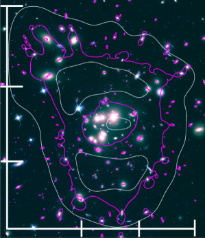
Figure 1.— False-color image of A1689 cluster (red: $i_{775}$, green: $V_{625}$, red: $B_{475}$). The critical lines for background sources at $z=2.5$ are shown with the magenta lines. The white curves are the contours indicating the $50$% sensitivity of the deepest part in the mosaic map. The white thick lines and ticks indicate the 9 regions of our noise estimates.

3. Data Analysis

We show our data analyses in the following subsections. The wavelengths of our mm maps fall in the range of $1.03-1.32$ mm. Our data set is composed of 63 Band 6 maps and 4 Band 7 maps (Table 2), and the majority of our data are taken with Band 6. Because our major data of the ALMA Band 6 maps have the average wavelength of 1.23 mm, we derive the number counts with a flux density at 1.2 mm, $S_{\rm 1.2mm}$. We scale the flux densities of our mm maps to $S_{\rm 1.2mm}$ with the flux density ratios summarized in Table 2. For the data of the previous studies defined with the wavelengths different from 1.2 mm, we estimate $S_{\rm 1.2mm}$ with the ratios of $S_{\rm 1.2mm}/S_{850\mu{\rm m}}=0.37$, $S_{\rm 1.2mm}/S_{870\mu{\rm m}}=0.39$, $S_{\rm 1.2mm}/S_{\rm 1.1mm}=0.77$, and $S_{\rm 1.2mm}/S_{\rm 1.3mm}=1.28$. All of these flux density ratios are calculated based on a modified blackbody whose spectral index $\beta_{\rm d}$ and dust temperature $T_{\rm d}$ are similar to those of typical SMGs; $\beta_{\rm d}=1.8$ (e.g., chapin2009, ; Planck Collaboration planck2011) and $T_{\rm d}=35$ K (e.g., kovacs2006; coppin2008). Here we assume a source redshift of $z=2.5$ that is a median redshift value of SMGs (e.g., chapman2005; yun2012; simpson2014).

3.1. Source Detection

We conduct source extraction for our ALMA maps before primary beam corrections with SExtractor version 2.5.0 (bertin1996). textcolorblue The source extraction is carried out in high sensitivity regions. For the single-pointing maps presented in Sections 2.1 and 2.2.1, we use the regions with the primary beam sensitivity greater than 50%. For the mosaic map shown in Section 2.2.2, we perform source extraction where the relative sensitivity to the deepest part of the mosaic map is greater than 50%.

We identify sources with a positive peak count above the 3.0$\sigma$ level, assuming the sources are not resolved out in our ALMA maps. The catalog of these sources is referred to as the 3.0$\sigma$-detection catalog. From our 3.0$\sigma$-detection catalog, we remove the objects located at the map centers that are main science targets of the archived-data ALMA observations.

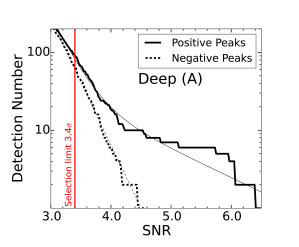
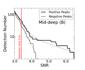
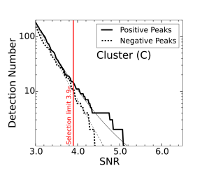
Figure 2.— Total numbers of positive and negative peaks in the deep (A), medium-deep (B), and cluster (C) sub-datasets as a function of SNR. The thick solid and dashed lines show the total numbers of the positive and negative peaks, respectively. The thin solid and dashed curves denote the best-fit model functions. The red lines are selection limits for our source catalog. See text for more details.

3.2. Spurious Sources and Source Catalog

The 3.0$\sigma$-detection catalog should include many spurious sources, because the detection is simply determined with a peak pixel count. To evaluate the number of the spurious sources, we conduct negative peak analysis (hatsukade2013; ono2014; carniani2015) for the deep (A), medium-deep (B), and cluster (C) datasets. We multiply $-1$ to each pixel value of our ALMA maps, and perform the source extraction for negative peaks in the same manner as those in Section 3.1. The numbers of negative and positive peaks in our ALMA maps are shown in Figure 2. The excess of the positive to negative peak numbers is regarded as the real source numbers. We model the negative and positive peak distributions of Figure 2 with the functions of signal-to-noise ratio SNR,

$${N_{\rm np}^{\rm c}} \ =\ a_{\rm n}\times 10^{-b_{\rm n}\times{\rm SNR}},$$ (1)

$${N_{\rm pp}^{\rm c}} \ =\ a_{\rm n}\times 10^{-b_{\rm n}\times{\rm SNR}}+a_{\rm p}\times 10^{-b_{\rm p}\times{\rm SNR}},$$ (2)

where $N_{\rm np}^{\rm c}$ and $N_{\rm pp}^{\rm c}$ are the cumulative numbers of negative and positive peaks, respectively, and $a_{\rm n}$, $b_{\rm n}$, $a_{\rm p}$, and $b_{\rm p}$ are free parameters.

We estimate spurious source rates $f_{\rm sp}$ defined by the ratio of negative to positive peak numbers,

$$f_{\rm sp}({\rm SNR}) \ =\ \frac{N_{\rm np}^{\rm c}({\rm SNR})}{N_{\rm pp}^{\rm c}({\rm SNR})}.$$ (3)

We evaluate $f_{\rm sp}$ with the best-fit functions of eqs. (1) and (2), and present $f_{\rm sp}$ in Figure 3.

Figures 3 indicates that the field data of deep (A) and medium-deep (B) have an almost identical distribution of the spurious source rates, while the cluster data (C) shows spurious source rates higher than (A) and (B) at a given SNR. This result would suggest that spurious source rates do not depend on the data depth, but the mapping modes. The complex distribution of the depths in the mapping data of (C) would have the relation of SNR and spurious source rate that is different from the smooth distribution of the depth in the single pointing data of (A) and (B). We use sources down to an SNR whose spurious source rate is $\lesssim 70$%, and adopt 3.4, 3.4, and $3.9\sigma$ levels for our selection limits of the data (A), (B), and (C), respectively. Applying these selection limits to our 3.0$\sigma$-detection catalog, we obtain a source catalog consisting of 133 sources: 122 from the field data (A and B) and 11 from the cluster data (C). The source catalog of our 133 faint ALMA sources is presented in Table LABEL:tab:our_catalog.

Note that A1689-zD1, an LBG at $z=7.5$ behind A1689 (watson2015), is not included in our source catalog because A1689-zD1 is located outside of the primary beam with a $>50\%$ sensitivity that is one of our selection criteria. Nevertheless, we have looked at the position of A1689-zD1 in our data, and found that there is a source with an SNR of 4 whose flux is the same as the one derived by watson2015 within the $\sim 1\sigma$ uncertainty. We confirm the ALMA source detection at the position of A1689-zD1.

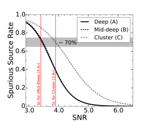
Figure 3.— Cumulative spurious source rates as a function of SNR. The solid, dashed, and dotted lines indicate the deep (A), medium-deep (B), and cluster (C) sub-datasets, respectively. The red lines at SNRs of 3.4 and 3.9 are the selection limits (SL) of our source catalog.

3.3. Completeness and Flux Boosting

We estimate the detection completeness by Monte-Carlo simulations. We put a flux-scaled synthesized beam into a map as an artificial source on a random position. These artificial sources have SNRs ranging from 3.0 to 7.0 with an SNR step of 0.2 dex. If an artificial source is extracted within a distance of the synthesized beam size from the input position, we regard that the source is recovered. These completeness estimations are conducted in the data before primary beam corrections, because we perform the source extractions in the real data (Section 3.1) uncorrected for primary beam attenuations. For all of our ALMA maps, we iterate this process 100 times at an SNR bin. Figure 4 displays our completeness estimates for three sub-datasets. We fit the function of $1-\exp(a{\rm SNR}-b)$ to our completeness estimates, where $a$ and $b$ are free parameters. The best-fit functions are also shown in Figure 4.

We examine the flux boosting that is caused by the confusions of the undetected faint sources (austermann2009; austermann2010). We use the detected objects of the Monte-Carlo simulations conducted for the completeness estimates, and measure the output flux densities at the input positions. We find that the ratios of the input to output flux densities are almost unity with a variance of only 5% over the wide SNR range of our ALMA maps. This small flux boosting is probably found, because the angular resolution of ALMA is high. We thus conclude that the effect of flux boosting is negligibly small.

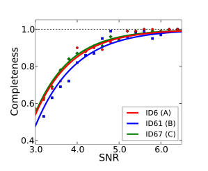
Figure 4.— Completeness as functions of SNR for three sub-datasets. The circles (red line), squares (blue line), and diamonds (green line) represent the completeness values (the best-fit functions) of the ID 6, 61 and 67 maps, respectively.

3.4. Flux Measurement

We estimate the source fluxes of our 133 objects from the integrated flux densities measured with the 2D Gaussian-fitting routine of $imfit$ in CASA. Because the integrated flux density values for low-SNR sources would include large systematic uncertainties originated from the spatially-correlated positive noise at around the source position, we use the integrated flux densities of $imfit$ only for the sources which are identified as ’resolved’ with an SNR of $\geq$ 5. For the rest of the sources, we use the peak fluxes of the $imfit$ best-fit Gaussian measurements. We confirm that the peak flux values of $imfit$, $S_{\rm imfit}$, agree with those of SExtractor, $S_{\rm SEx}$, within the 1$\sigma$ error, $S_{\rm imfit}/S_{\rm SEx}=0.93\pm 0.15$.

Because the sources in the cluster data of A1689 would be distorted by the gravitational lensing effects, we make a low-resolution map of A1689 produced with a $1^{\prime\prime}$ circular gaussian uv-taper that is the same as the one produced by watson2015. The taped beam size is $1\farcs 31\times 1\farcs 12$. In this map, we perform the $imfit$ flux measurements (as described above) at the source positions determined in the original map. Here we define flux measurements in the tapered and non-tapered maps as $S_{\rm taper}$ and $S_{\rm no\,taper}$, respectively. We then obtain $S_{\rm taper}/S_{\rm no\,taper}=1.01\pm 0.19$ on average, if we omit two sources showing signatures of source confusions by neighboring objects. However, the strongly-lensed source of A1 shows a systematically high fraction of $S_{\rm taper}$ / $S_{\rm no\,taper}=1.23$. Thus, we decide to use $S_{\rm taper}$ for the cluster data of A1689, except for those two confusion sources. We also make low-resolution maps for some of the field data, and perform the same test of tapering. Because we find that $S_{\rm taper}$ and $S_{\rm no\,taper}$ are almost identical in these data, we use $S_{\rm no\,taper}$ for the field data.

We test the reliability of our flux measurements, performing flux recovery simulations. First, we select the typical data sets of ID22 and ID55 that have beam sizes of $\sim 0\farcs 8$ and $\sim 1\farcs 2$ corresponding to the two peaks of bimodal size distribution for our data. We then create 200 input sources of elliptical Gaussian model profiles with the uniform distribution of SNRs in $3-7$ and major-axis sizes of $0\farcs 2$ and $0\farcs$5. Here, the input source sizes are chosen from recent ALMA high-resolution studies. ikarashi2014 and simpson2015a claim that the median sizes of individual submm sources are $\sim 0\farcs 2-0\farcs 3$ in FWHM. simpson2015a also find that the stacked image of submm sources with a low SNR of $4-5$ has the size of FWHM $0\farcs 35^{+0.17}_{-0.10}$. Thus, we investigate the model sources of $0\farcs 2$ and $0\farcs 5$ that are taken from the median individual source size and the 1$\sigma$ upper limit stacked source size. We add these model sources to ID22 and ID55 maps at random positions. Finally, we obtain flux densities of the model sources in the same manner as our flux measurements for the real sources, and compare these flux measurements with the input source fluxes. In the case of the $0\farcs 2$ input source size, we find that the flux recovery ratio (defined by the ratio of the output to input fluxes) is $1.0\pm 0.1$ ($1.0\pm 0.2$) for ID22 (ID55) data. Similarly, in the case of the $0\farcs 5$ input source size, we obtain $0.8\pm 0.1$ ($0.9\pm 0.2$) for ID22 (ID55) data. These results suggest that the flux recovery ratios are nearly unity within the $1-2\sigma$ uncertainties, and that our flux measurements are reliable.

Note that missing fluxes of interferometric observations are negligible. ALMA proposer’s guide shows that there exist missing flux effects for sources with $\simeq 2\farcs 0-3\farcs 0$ at Band 6/7 for the shortest-baseline configuration that we use. The source sizes of $\simeq 2\farcs 0-3\farcs 0$ are significantly larger than our ALMA sources whose angular sizes are $\lesssim 0\farcs 5$, and the missing fluxes should be negligible.

Source Catalog 1	1	337.049805	-35.169643	0.06 $\pm$ 0.02	0.07 $\pm$ 0.02	3.6	0.57
2	1	337.050232	-35.164864	0.41 $\pm$ 0.01	0.68 $\pm$ 0.07	39.3	0.00
3	1	337.050293	-35.170044	0.07 $\pm$ 0.02	0.09 $\pm$ 0.02	4.0	0.34
4	1	337.053314	-35.165119	0.06 $\pm$ 0.01	0.12 $\pm$ 0.02	5.7	0.00
5	1	337.054413	-35.167576	0.05 $\pm$ 0.01	0.07 $\pm$ 0.02	4.1	0.27
6	1	337.054718	-35.166332	0.05 $\pm$ 0.01	0.06 $\pm$ 0.02	3.5	0.66
7	2	148.887314	18.150942	0.05 $\pm$ 0.01	0.04 $\pm$ 0.02	3.6	0.63
8	2	148.891403	18.151211	0.06 $\pm$ 0.02	0.06 $\pm$ 0.02	3.4	0.71
9	3	34.446007	-5.008159	0.05 $\pm$ 0.01	0.05 $\pm$ 0.02	3.5	0.70
10	3	34.446648	-5.007715	0.05 $\pm$ 0.01	0.04 $\pm$ 0.02	3.4	0.70
11	4	34.437332	-5.492185	0.06 $\pm$ 0.02	0.04 $\pm$ 0.01	3.7	0.53
12	4	34.437649	-5.494778	0.06 $\pm$ 0.02	0.03 $\pm$ 0.01	3.5	0.67
13	4	34.437805	-5.494339	0.06 $\pm$ 0.01	0.03 $\pm$ 0.01	3.8	0.48
14	4	34.439056	-5.494986	0.06 $\pm$ 0.02	0.03 $\pm$ 0.01	3.6	0.60
15	4	34.440075	-5.494945	0.07 $\pm$ 0.02	0.04 $\pm$ 0.01	3.6	0.63
16	5	121.593948	-41.376675	0.10 $\pm$ 0.03	0.08 $\pm$ 0.04	3.6	0.60
17	5	121.596870	-41.375671	0.06 $\pm$ 0.02	0.08 $\pm$ 0.02	3.6	0.63
18	5	121.599480	-41.373417	0.08 $\pm$ 0.02	0.10 $\pm$ 0.03	3.7	0.55
19	5	121.599564	-41.375568	0.07 $\pm$ 0.02	0.08 $\pm$ 0.03	3.6	0.61
20	5	121.600471	-41.375629	0.08 $\pm$ 0.02	0.09 $\pm$ 0.03	3.6	0.60
21	7	336.940674	-35.119549	0.11 $\pm$ 0.03	0.13 $\pm$ 0.04	3.8	0.48
22	8	201.001526	27.413574	0.10 $\pm$ 0.03	0.11 $\pm$ 0.04	3.5	0.70
23	8	201.001526	27.413574	0.10 $\pm$ 0.03	0.11 $\pm$ 0.04	3.5	0.70
24	8	201.001526	27.413574	0.10 $\pm$ 0.03	0.11 $\pm$ 0.04	3.5	0.70
25	9	325.760986	6.904217	0.13 $\pm$ 0.04	0.17 $\pm$ 0.05	3.5	0.68
26	9	325.762177	6.902022	0.14 $\pm$ 0.04	0.17 $\pm$ 0.05	3.6	0.62
27	9	325.763336	6.905892	0.08 $\pm$ 0.02	0.10 $\pm$ 0.03	3.4	0.72
28	9	325.767029	6.902850	0.15 $\pm$ 0.04	0.16 $\pm$ 0.05	3.6	0.60
29	10	352.281616	-3.033988	0.13 $\pm$ 0.04	0.12 $\pm$ 0.04	3.4	0.71
30	10	352.284851	-3.031080	0.16 $\pm$ 0.03	0.16 $\pm$ 0.03	5.9	0.00
31	10	352.285248	-3.030138	0.17 $\pm$ 0.04	0.17 $\pm$ 0.04	4.6	0.08
32	10	352.285309	-3.035150	0.11 $\pm$ 0.03	0.10 $\pm$ 0.03	3.8	0.47
33	11	200.929321	27.340736	0.15 $\pm$ 0.04	0.13 $\pm$ 0.04	3.9	0.40
34	12	150.547440	1.910628	0.13 $\pm$ 0.04	0.13 $\pm$ 0.05	3.7	0.55
35	13	351.831116	6.267834	0.13 $\pm$ 0.03	0.12 $\pm$ 0.03	4.2	0.22
36	13	351.833496	6.267574	0.16 $\pm$ 0.04	0.15 $\pm$ 0.04	3.7	0.53
37	14	13.760888	1.771644	0.10 $\pm$ 0.03	0.08 $\pm$ 0.02	4.0	0.35
38	14	13.761566	1.768838	0.16 $\pm$ 0.04	0.12 $\pm$ 0.04	3.7	0.52
39	14	13.763390	1.770106	0.11 $\pm$ 0.03	0.08 $\pm$ 0.03	3.7	0.52
40	14	13.764014	1.770272	0.13 $\pm$ 0.03	0.09 $\pm$ 0.03	3.7	0.50
41	15	149.775772	1.736944	0.16 $\pm$ 0.03	0.18 $\pm$ 0.04	5.1	0.02
42	15	149.775955	1.738510	0.15 $\pm$ 0.04	0.17 $\pm$ 0.05	3.9	0.41
43	15	149.776794	1.736661	0.09 $\pm$ 0.03	0.07 $\pm$ 0.03	3.6	0.63
44	18	337.254547	14.950516	0.17 $\pm$ 0.05	0.14 $\pm$ 0.04	3.8	0.48
45	18	337.256073	14.954236	0.19 $\pm$ 0.03	0.21 $\pm$ 0.03	6.1	0.00
46	19	149.722565	2.606706	0.11 $\pm$ 0.03	0.10 $\pm$ 0.04	3.4	0.70
47	19	149.724045	2.602218	0.21 $\pm$ 0.05	0.28 $\pm$ 0.07	4.1	0.26
48	20	149.792572	2.103762	0.12 $\pm$ 0.03	0.10 $\pm$ 0.04	4.0	0.30
49	21	32.553406	-4.939113	0.12 $\pm$ 0.03	0.11 $\pm$ 0.03	3.9	0.37
50	21	32.553787	-4.939454	0.11 $\pm$ 0.03	0.15 $\pm$ 0.03	3.7	0.56
51	21	32.555397	-4.937203	0.13 $\pm$ 0.03	0.13 $\pm$ 0.04	3.7	0.54
52	22	150.127991	2.288839	0.13 $\pm$ 0.04	0.08 $\pm$ 0.03	3.4	0.72
53	23	359.017120	19.607481	0.10 $\pm$ 0.03	0.08 $\pm$ 0.03	3.4	0.71
54	24	150.406784	2.034714	0.14 $\pm$ 0.04	0.12 $\pm$ 0.04	3.5	0.64
55	25	150.393936	1.998264	0.15 $\pm$ 0.04	0.16 $\pm$ 0.05	3.7	0.56
56	26	34.100346	-5.154171	0.15 $\pm$ 0.04	0.14 $\pm$ 0.05	3.5	0.64
57	26	34.100658	-5.156616	0.16 $\pm$ 0.05	0.17 $\pm$ 0.06	3.5	0.66
58	26	34.102978	-5.155593	0.15 $\pm$ 0.04	0.15 $\pm$ 0.05	3.4	0.70
59	27	34.034069	-5.104988	0.17 $\pm$ 0.04	0.18 $\pm$ 0.06	3.8	0.45
60	28	34.472076	-4.711596	0.26 $\pm$ 0.07	0.27 $\pm$ 0.09	3.5	0.65
61	28	34.473747	-4.713997	0.16 $\pm$ 0.04	0.20 $\pm$ 0.06	3.6	0.62
62	29	34.392979	-5.043759	0.17 $\pm$ 0.04	0.19 $\pm$ 0.06	3.7	0.51
63	29	34.396526	-5.042582	0.21 $\pm$ 0.06	0.23 $\pm$ 0.07	3.6	0.59
64	29	34.396526	-5.046781	0.25 $\pm$ 0.07	0.26 $\pm$ 0.09	3.4	0.72
65	31	34.612003	-4.588018	0.25 $\pm$ 0.07	0.28 $\pm$ 0.08	3.5	0.69
66	31	34.612686	-4.583063	0.36 $\pm$ 0.07	0.43 $\pm$ 0.09	4.9	0.04
67	31	34.613739	-4.588505	0.31 $\pm$ 0.09	0.31 $\pm$ 0.10	3.5	0.68
68	31	34.613930	-4.585264	0.19 $\pm$ 0.06	0.18 $\pm$ 0.06	3.5	0.70
69	33	34.272991	-4.859830	0.29 $\pm$ 0.08	0.34 $\pm$ 0.11	3.5	0.68
70	33	34.274231	-4.860201	0.32 $\pm$ 0.09	0.43 $\pm$ 0.12	3.6	0.59
71	33	34.274761	-4.859237	0.26 $\pm$ 0.07	0.32 $\pm$ 0.09	3.8	0.46
72	34	34.305080	-5.067344	0.29 $\pm$ 0.07	0.39 $\pm$ 0.10	3.9	0.41
73	34	34.305538	-5.069685	0.23 $\pm$ 0.06	0.33 $\pm$ 0.09	3.6	0.61
74	34	34.305553	-5.067293	0.29 $\pm$ 0.07	0.22 $\pm$ 0.09	4.2	0.19
75	34	34.307556	-5.071889	0.33 $\pm$ 0.09	0.48 $\pm$ 0.12	3.6	0.61
76	34	34.309822	-5.069085	0.29 $\pm$ 0.08	0.23 $\pm$ 0.11	3.5	0.65
77	35	230.738800	-0.125928	0.35 $\pm$ 0.10	0.23 $\pm$ 0.07	3.5	0.69
78	35	230.739777	-0.125576	0.28 $\pm$ 0.08	0.20 $\pm$ 0.06	3.6	0.59
79	35	230.743118	-0.127994	0.28 $\pm$ 0.08	0.18 $\pm$ 0.06	3.5	0.66
80	36	34.327038	-5.131583	0.21 $\pm$ 0.06	0.27 $\pm$ 0.09	3.8	0.48
81	37	34.401154	-5.152167	0.33 $\pm$ 0.10	0.37 $\pm$ 0.15	3.4	0.72
82	37	34.401531	-5.154098	0.30 $\pm$ 0.08	0.34 $\pm$ 0.13	3.7	0.55
83	37	34.403275	-5.149917	0.36 $\pm$ 0.11	0.61 $\pm$ 0.18	3.4	0.71
84	38	231.036255	-0.176025	0.39 $\pm$ 0.11	0.22 $\pm$ 0.08	3.5	0.67
85	38	231.037949	-0.178142	0.22 $\pm$ 0.06	0.15 $\pm$ 0.04	3.7	0.54
86	40	34.414261	-5.201880	0.34 $\pm$ 0.10	0.56 $\pm$ 0.16	3.5	0.65
87	40	34.419544	-5.199385	0.31 $\pm$ 0.08	0.52 $\pm$ 0.14	3.8	0.46
88	41	149.590530	2.807018	0.28 $\pm$ 0.07	0.23 $\pm$ 0.05	4.2	0.21
89	41	149.591949	2.805352	0.26 $\pm$ 0.07	0.21 $\pm$ 0.05	4.0	0.31
90	42	150.688171	2.681118	0.37 $\pm$ 0.07	0.26 $\pm$ 0.06	5.4	0.01
91	45	34.194702	-5.056259	0.43 $\pm$ 0.12	0.39 $\pm$ 0.15	3.5	0.71
92	45	34.197121	-5.059778	0.31 $\pm$ 0.08	0.37 $\pm$ 0.10	3.7	0.55
93	46	150.409714	2.358208	0.30 $\pm$ 0.09	0.32 $\pm$ 0.09	3.5	0.71
94	47	149.770050	1.804996	0.32 $\pm$ 0.09	0.31 $\pm$ 0.10	3.4	0.72
95	48	34.411190	-4.745051	0.30 $\pm$ 0.08	0.14 $\pm$ 0.09	3.8	0.44
96	48	34.411701	-4.745893	0.31 $\pm$ 0.08	0.34 $\pm$ 0.09	4.0	0.31
97	49	150.600494	2.444365	0.47 $\pm$ 0.13	0.53 $\pm$ 0.14	3.6	0.59
98	51	34.440269	-4.912953	0.39 $\pm$ 0.11	0.40 $\pm$ 0.12	3.6	0.60
99	51	34.441357	-4.912045	0.32 $\pm$ 0.08	0.29 $\pm$ 0.09	3.9	0.43
100	51	34.441635	-4.913539	0.46 $\pm$ 0.13	0.45 $\pm$ 0.14	3.6	0.62
101	51	34.442795	-4.911066	0.53 $\pm$ 0.08	0.56 $\pm$ 0.11	6.2	0.00
102	51	34.443920	-4.909602	0.41 $\pm$ 0.12	0.35 $\pm$ 0.13	3.5	0.65
103	52	150.151459	1.751314	0.49 $\pm$ 0.14	0.50 $\pm$ 0.13	3.6	0.64
104	54	34.759140	-4.832398	0.32 $\pm$ 0.09	0.37 $\pm$ 0.11	3.5	0.71
105	55	150.022736	2.027032	0.53 $\pm$ 0.08	0.46 $\pm$ 0.08	6.8	0.00
106	57	34.141144	-5.232085	0.47 $\pm$ 0.13	0.42 $\pm$ 0.15	3.6	0.60
107	58	34.303791	-5.161064	0.47 $\pm$ 0.14	0.58 $\pm$ 0.16	3.4	0.73
108	59	150.201645	2.021740	0.57 $\pm$ 0.15	0.72 $\pm$ 0.22	3.7	0.53
109	60	34.250214	-4.804325	0.34 $\pm$ 0.09	0.34 $\pm$ 0.10	3.9	0.39
110	60	34.250927	-4.802006	0.37 $\pm$ 0.11	0.39 $\pm$ 0.13	3.5	0.68
111	61	34.744495	-4.855921	0.35 $\pm$ 0.10	0.27 $\pm$ 0.12	3.5	0.70
112	61	34.747295	-4.858103	0.37 $\pm$ 0.10	0.26 $\pm$ 0.11	3.8	0.45
113	62	150.757401	1.700786	0.50 $\pm$ 0.14	0.57 $\pm$ 0.21	3.5	0.70
114	62	150.758331	1.703298	0.42 $\pm$ 0.12	0.52 $\pm$ 0.17	3.6	0.60
115	62	150.760971	1.703856	1.01 $\pm$ 0.10	1.17 $\pm$ 0.18	9.7	0.00
116	62	150.762024	1.698676	0.57 $\pm$ 0.16	0.85 $\pm$ 0.24	3.5	0.69
117	62	150.762161	1.701653	0.34 $\pm$ 0.10	0.37 $\pm$ 0.14	3.5	0.68
118	62	150.762741	1.700690	0.43 $\pm$ 0.12	0.61 $\pm$ 0.17	3.6	0.62
119	62	150.763138	1.702965	0.47 $\pm$ 0.13	0.70 $\pm$ 0.19	3.6	0.62
120	64	34.587593	-5.318766	0.32 $\pm$ 0.09	0.21 $\pm$ 0.10	3.6	0.59
121	64	34.589180	-5.315989	0.61 $\pm$ 0.17	0.69 $\pm$ 0.21	3.5	0.65
122	65	34.387825	-5.220457	0.41 $\pm$ 0.11	0.42 $\pm$ 0.13	3.7	0.51
123	67	197.860764	-1.337225	0.25 $\pm$ 0.06	0.03 $\pm$ 0.01	4.3	0.53
124	67	197.862061	-1.342226	0.24 $\pm$ 0.06	0.00 $\pm$ 0.00	4.3	0.54
125	67	197.864731	-1.343368	0.27 $\pm$ 0.06	0.03 $\pm$ 0.01	4.7	0.32
126	67	197.869086	-1.337143	0.31 $\pm$ 0.08	0.08 $\pm$ 0.03	4.1	0.60
127	67	197.871590	-1.345783	0.30 $\pm$ 0.06	0.02 $\pm$ 0.01	5.1	0.20
128	67	197.874725	-1.326138	0.22 $\pm$ 0.05	0.02 $\pm$ 0.01	4.3	0.51
129	67	197.881638	-1.323127	0.26 $\pm$ 0.05	0.05 $\pm$ 0.02	4.8	0.29
130	67	197.882812	-1.356609	0.28 $\pm$ 0.07	0.05 $\pm$ 0.02	4.1	0.64
131	67	197.883881	-1.355241	0.30 $\pm$ 0.08	0.06 $\pm$ 0.03	4.0	0.65
132	67	197.884125	-1.334885	0.30 $\pm$ 0.07	0.13 $\pm$ 0.05	4.2	0.58
133	67	197.886185	-1.328756	0.24 $\pm$ 0.05	0.04 $\pm$ 0.01	5.1	0.19

3.5. Mass Model

We construct a mass model for the cluster data (C) of A1689 at $z=0.183$. We make the mass model with the parametric gravitational lensing package GLAFIC (oguri2010) in the same manner as ishigaki2015. Our mass model consists of three types of mass distributions: cluster-scale halos, cluster member galaxy halos, and external perturbation. For evaluating the mass distributions, we make a galaxy catalog of A1689, conducting source extractions in the optical images of $g_{475},\ r_{625},$ and $i_{775}$ bands taken with $Hubble\ Space\ Telescope$ (HST). The cluster-scale halos are estimated with three brightest member galaxies in the core of the cluster. The cluster member galaxies are selected by the color criteria of

$$r_{625} \ <\ 24,$$ (4)

$$g_{475}-r_{625} \ <\ -\frac{1}{18}(r_{625}-24)+1.3,$$

$$g_{475}-r_{625} \ >\ -\frac{1}{18}(r_{625}-24)+0.7,$$

where the source extraction and photometry are carried out with SExtractor. The external perturbation is calculated with the theoretical model under the assumption that the perturbation is weak (e.g., kochanek1991).

Using the positions of the multiple images presented in the literature (coe2010; diego2015), we optimize free parameters of the mass profiles based on the standard $\chi^{2}$ minimization to determine the best-fit mass model. Figure 1 presents the best-fit mass model. The best-fit mass model achieves that all of the offsets between the model and observed positions of multiple images are within $1\farcs 0$ in the image plane. We then calculate magnification factors $\mu$ at the positions of our sources. For the $\mu$ estimates, we assume our source redshift of $z=2.5$ that is the same as the one used in the flux scaling shown in Section 3. This assumption does not change our statistical results, because most of mm sources in the target fields at the high-galactic latitude should reside at $z>1$ where the $\mu$ values do not depend much on a redshift. Here we calculate the magnification factors for sources at $z=7.5$ that correspond to the redshift of A1689-zD1, and evaluate the differences between the magnification factors for sources at $z=2.5$ ($\mu_{2.5}$) and $z=7.5$ ($\mu_{7.5}$). We find that the average difference, $\Delta\mu\equiv(\mu_{7.5}-\mu_{2.5})/\mu_{2.5}$, is $0.36\pm 0.25$ for our 11 sources in A1689. Although the difference is not large, we include the lensing magnification difference of $0.36$ into the errors of the intrinsic flux estimates for our 11 sources in A1689. Accordingly, we propagate these uncertainties to our major results such as number counts shown in Section 4.

3.6. Survey Area

We estimate survey areas of our data of A, B, and C, and present these estimates in Figure 5. The survey areas are defined by the high sensitivity regions that are detailed in Section 3.1. Because the sensitivities of our ALMA maps are not spatially uniform, the survey areas depend on the flux densities.

In the field data of A and B, the sensitivity of the primary beam decreases with increasing radius from a map center. In other words, the detectable intrinsic flux densities (corrected for the primary beam attenuation) increase from the center to the edge of the data. First, we find the radius where sources with the intrinsic flux densities can be detected at our selection limit SNR. Then, we calculate areas with the radius given in each map, and sum up these areas to obtain the total survey areas.

In the cluster data of C, the spatial distribution of the sensitivity is not expressed by a simple function of radius, because the cluster data are taken by mosaic mapping. Moreover, there are cluster-lensing magnification effects that allow us to detect intrinsically faint sources. We make an effective magnification map, multiplying, at each position, the sensitivity and the magnification factor estimated with the mass model of Section 3.5. We then calculate the survey area of the C data where a source with an intrinsic flux density can be observed above the selection limit.

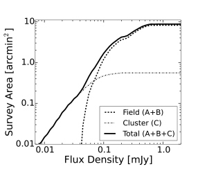
Figure 5.— Survey areas as a function of intrinsic flux densities. The dashed, dotted, and solid lines represent the survey areas of the field (A and B), cluster (C), and total (A, B, and C) datasets, respectively.

4. Number Counts and EBL

4.1. Number Counts at 1.2 mm

We derive differential number counts at 1.2 mm. For the number counts, we use the 122 sources identified in the ALMA Band 6 maps covering the 1.2 mm band, because there is a possibility that the 11 sources in the Band 7 would include unknown systematics in the flux scaling to 1.2 mm fluxes (Section 3). To derive the number counts, we basically follow the methods used in the previous ALMA studies (hatsukade2013; ono2014; carniani2015). A contribution from an identified source with an intrinsic flux density of $S$ to the number counts, $\xi$, is determined by

$$\xi(S)=\frac{1-f_{\rm sp}(S)}{C(S)A_{\rm eff}(S)},$$ (5)

where $C$ is the completeness, and $A_{\rm eff}$ is the survey area. For C, $A_{\rm eff}$, and $f_{\rm sp}$ (eq.3), we use the values derived in Section 3. Then, we calculate a sum of the contributions for each flux bin,

$$n(S)=\frac{\Sigma\xi(S)}{\Delta\log S},$$ (6)

where $\Delta\log S$ is the scaling factor of $0.25$ for the 1-dex width logarithmic differential number counts. We estimate the errors that include both Poisson statistical errors of the source numbers and flux uncertainties of the identified sources. Because the numbers of our sources are small, we use the Poisson uncertainty values presented in gehrels1986 that are applicable for the small number statistics. The flux uncertainties are composed of the random noise and the ALMA system’s flux measurement uncertainty whose typical value is $\sim$10% (Section 2.3). Moreover, for our 11 sources in the A1689 data, the intrinsic flux estimates include the lensing magnification uncertainties (see Section 3.5). To evaluate these flux uncertainties, we perform Monte-Carlo simulations. We make a mock catalog of the faint ALMA sources whose flux densities follow the Gaussian probability distributions whose standard deviations are given by the combination of the random noise and the system (+ the lensing magnification) uncertainties. We obtain the number counts for each mock catalog in the same manner as those for our real sources. We repeat this processes 1000 times, and calculate the standard deviation of the number counts per flux bin caused by the flux uncertainties. Combining the standard deviation of the flux uncertainties with the Poisson errors, we finally obtain the $1\sigma$ uncertainties of the number counts.

The differential number counts and the associated $1\sigma$ uncertainties are shown in Figure 6 and Table 4. With the technique same as those deriving the differential number counts, we estimate the cumulative number counts that are summarized in Table 4.

In Figure 6, we find that the faintest data point at $\sim 0.002$ mJy (red open circle) is composed of a source with a very high magnification factor of $\mu>100$. The highly magnified sources would potentially include large systematic uncertainties originated from the mass modeling. Moreover, the faintest data point has the large error bar that does not provide important constraints on the number count measurements. Thus, we do not use the faintest data point in the following discussion. Except for this very high magnification factor object, the faintest and brightest sources in our sample have intrinsic fluxes of 0.018 and 1.2 mJy, respectively. Thus, our study covers the flux density range of $\sim 0.02-1$ mJy.

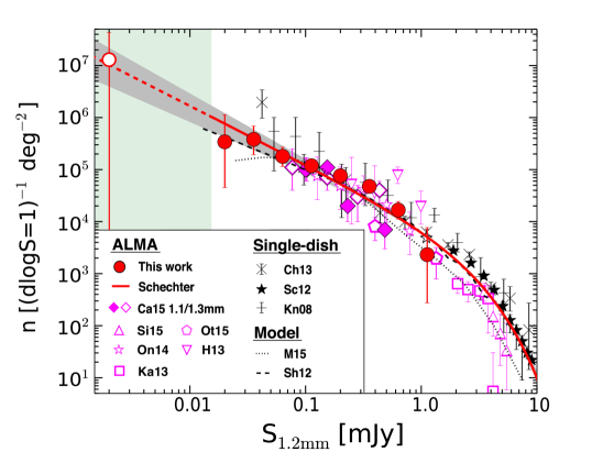
Figure 6.— Differential number counts at 1.2 mm. The red filled circles are our number counts derived from our faint ALMA sources. The red curve and the gray region denote the best-fit Schechter function and the associated $1\sigma$ error. In the Schechter function fitting, we use our number counts and the previous measurements shown with the black filled stars (Sc12; scott2012) and the magenta filled diamonds (Ca15 1.1 mm; carniani2015). Note that the 1.1 mm results of Ca15 are obtained from ALMA sources, none of which are used in our number count measurements. Because the rest of the existing ALMA studies include some ALMA data covered by our study, for our Schechter function fitting we do not include the previous ALMA measurements shown with the magenta open squares (Ka13; karim2013), open inverse triangles (H13; hatsukade2013), open stars (O14; ono2014), open diamonds (Ca15 1.3 mm; carniani2015), open triangles (Si15; simpson2015b), and open pentagons (Ot15; oteo2015). Note that the faintest data point of our study (red open circle) is also removed from the sample of our Schether function fitting, due to the possible large systematic uncertainties. The pale-green region presents a flux range where no reliable number-count data bin exists (see text). We do not use the faintest data point of Sc12 (black open star) for our fitting, because this data point has unrealisticly small errors. The dashed and dotted curves show the model predictions for number counts based on cosmological hydrodynamic simulations with GADGET-3 (Sh12; shimizu2012) and semi-analytic models (M15; makiya2015), respectively. These model predictions are roughly consistent with our results. For the previous measurements of the number counts at 1.1 mm and 1.3 mm different from our 1.2 mm band, we scale the flux densities with the methods shown in Section 3. Since the flux scaling factors for $<1$ mm wavelengths would contain relatively large systematic uncertainties, we do not use the $<1$ mm band data, for our Schechter function fitting, that are presented with the open triangles (Kn08; knudsen2008) and open hexagons (Ch13; chen2013).

Table 4Differential and Cumulative Number Counts at $1.2$ mm

$S$	$\log(n)$	$N_{\rm diff}$
(mJy)	([$\Delta\log S=1$]-1deg-2 )
(0.002)	$7.1_{-7.1}^{+0.5}$	1
0.020	$5.5_{-0.5}^{+0.3}$	2
0.036	$5.6_{-0.4}^{+0.3}$	6
0.063	$5.3_{-0.4}^{+0.2}$	15
0.112	$5.1_{-0.2}^{+0.2}$	25
0.200	$4.9_{-0.2}^{+0.1}$	27
0.356	$4.7_{-0.2}^{+0.1}$	29
0.633	$4.2_{-0.2}^{+0.2}$	15
1.124	$3.4_{-1.3}^{+0.5}$	2
$S$	$\log(n(>S))$	$N_{\rm cum}$
(mJy)	(deg-2)
(0.002)	$6.6_{-1.1}^{+0.5}$	122
0.015	$5.5_{-0.4}^{+0.3}$	121
0.027	$5.3_{-0.3}^{+0.2}$	119
0.047	$5.0_{-0.2}^{+0.2}$	113
0.084	$4.8_{-0.2}^{+0.1}$	98
0.150	$4.6_{-0.1}^{+0.1}$	73
0.267	$4.2_{-0.2}^{+0.2}$	46
0.474	$3.7_{-0.3}^{+0.2}$	17
0.843	$2.8_{-0.5}^{+0.6}$	2

Note. — (1): Source ID. (2): Map ID that corresponds to the one in Table 2. (3): Peak flux density of the SExtractor measurement (Section 3.1) with the primary beam correction at the observed wavelength. (4): The best-estimate source flux density at 1.2 mm. The source flux is estimated with the 2D Gaussian-fitting routine of imfit in CASA (Section 3.4) with the primary beam correction and the flux scaling to 1.2 mm (Section 3). For the sources found in the cluster data, the lensing magnification corrections are also applied (Section 3.5). The lensing magnification factors are estimated at the ALMA flux peak positions. The error bar includes the random noise, 10% of ALMA system’s flux measurement uncertainty, and the lensing magnification uncertainty (Section 4.1). (5): Signal-to-noise ratio of the peak flux density. (6): Spurious source rate that is defined by eq. 3. ^† Source identified in the Band 7 map. Unless otherwise specified, the source is found in the Band 6 map. ^‡ The lensing magnification is corrected. The ID 124 source has $0.0020\pm 0.0010$ mJy for the best-estimate source flux density at 1.2 mm with the primary-beam and lensing-magnification corrections.

Note. — The $1\sigma$ uncertainties are estimated from the combination of the number-count Poisson statistical errors and the flux uncertainties (see text). The column of $N_{\rm diff}$ presents the numbers of our 1.2 mm sources in each flux bin, while the one of $N_{\rm cum}$ denotes the cumulative source numbers down to the flux densities. For our analysis, we do not use the faintest bin data indicated with the parentheses (see text).

4.2. Comparison with Previous Number Count Measurements

We compare our number counts to previous measurements at the $\sim 1.2$ mm band. In the flux range close to our study, there are two types of previous studies, blank-field observations with ALMA and cluster observations for lensed sources with single-dish telescopes. For the measurements of 1.1 and 1.3 mm bands that are different from 1.2 mm band, we scale the flux densities with the methods described in Section 3.

4.2.1 Blank-Field Observations

To derive number counts, hatsukade2013 and ono2014 use 20 ALMA maps in one blank field of SXDS and 10 ALMA maps in 10 independent fields, respectively. carniani2015 obtain number counts with the 18 ALMA maps composed of 9 independent fields at 1.1 mm band and the 9 ALMA maps in one blank field of Cosmic Evolution Survey (COSMOS; scoville2007) at 1.2 mm band. After the flux density scaling, all of these previous number counts agree with our measurements within the $1\sigma$ uncertainties. Because the amount of our ALMA data is much larger than the previous studies, the statistical and systematic uncertainties of the number counts measurements are significantly smaller than those of previous studies.

4.2.2 Cluster Observations for Lensed Sources

Single-dish observations of SCUBA and SCUBA-2 for lensed sources behind galaxy clusters successfully reach the intrinsic flux limits comparable to the previous ALMA blank field observations. knudsen2008 conduct SCUBA observations for 12 clusters, and derive the number counts at 850 $\mu$m with the sample of 15 gravitationally lensed faint sources with flux densities below the SCUBA’s blank-field confusion limit ($\sim 2$ mJy at 850 $\mu$m). chen2013 observe 2 clusters as well as 3 blank fields with SCUBA-2, and obtain the number counts similar to those of knudsen2008. The number counts from these previous studies are also shown in Figure 6. These previous results generally agree with our results within the $1\sigma$ errors. Although the number counts of the previous studies are slightly higher than ours systematically at $\lesssim 0.1$ mJy, these small systematic differences would be explained by the uncertainties of the flux scaling from $850\mu$m to 1.2 mm.

4.3. Contributions to the EBL

In Section 4.1, we obtain the 1.2-mm number counts with our faint ALMA source. Because our sample lacks sources brighter than 1.2 mJy, we use previous studies of bright sources in the literature to investigate the source contributions to the IR EBL. There are a number of studies that investigate the bright sources (Figure 6), but we use the number counts at $2-10$ mJy obtained from a survey for six blank fields with a single-dish telescope instrument of AzTEC (scott2012), which shows reliable number counts at 1.1 mm that is close to 1.2 mm band . Although there is another systematic survey for bright sources from the single-dish observations with LABOCA (weiss2009), we do not use their data for our analysis, due to their observation wavelength of $870\ \mu$m far from our 1.2 mm band. It should be noted that the number counts of bright sources are still under debate (e.g., karim2013; chen2013; simpson2015b), because the recent high-resolution ALMA observations reveal multiple sources in a beam of single-dish observations (hodge2013). Nevertheless, our results below do not depend on the bright-source number counts, because the contribution from the bright sources is not large (Section 1).

The source contributions to the IR EBL can be calculated by integrating the number counts down to a flux density limit. To characterize the shape of the number counts, we use the Schechter function form (schechter1976) in the same manner as the previous studies,

$$\phi(S)dS=\phi_{*}\left(\frac{S}{S_{*}}\right)^{\alpha}\rm exp\it\left(-\frac{S}{S_{*}}\right)d\left(\frac{S}{S_{*}}\right),$$ (7)

where $\phi_{*}\rm$, $S_{*}$, and $\alpha$ are the normalization, characteristic flux density, and faint-end slope power-law index, respectively. The logarithmic form of $n(S)d(\rm log\it S)=\phi(S)dS$ is given by

$$n(S)=(\rm ln\ 10)\it\phi_{*}\left(\frac{S}{S_{*}}\right)^{(\alpha+1)}\rm\exp\it\left(-\frac{S}{S_{*}}\right).$$ (8)

Using eq. (8), we conduct $\chi^{2}$-fitting to the differential number counts derived from our and the previous observations shown with the filled symbols in Figure 6 that are our measurements and the AzTEC (scott2012) and ALMA 1.1 mm (carniani2015) results. Here we do not use the measurements of hatsukade2013, ono2014, oteo2015, and the 1.3 mm results of carniani2015 that are presented with the open symbols of Figure 6, because these studies use ALMA data covered by our study or the sample that does not meet our selection criteria (Section 2.2). We confirm that the entire ALMA 1.1 mm data of carniani2015 are different from ours. Including the bright number counts at $2-10$ mJy (see above), we perform Schechter function fitting with our number counts and those from the 1.1-mm observations with AzTEC (scott2012) and ALMA (carniani2015). We vary three Schechter parameters, and search for the best-fit parameter set of ($\phi_{*}$,$S_{*}$,$\alpha$) that minimizes $\chi^{2}$. The best-fit function and parameter set are presented in Figure 6 and Table 5, respectively. Figure 6 and the $\chi^{2}/dof$ of 16.9/19 (Table 5) indicate that the number counts are well represented by the Schechter function down to $\sim 0.02$ mJy.

We also carry out fitting of the double-power law (DPL) function in the same manner as the Schechter function fitting. The DPL function has four free parameters of $\phi_{*}^{\rm DPL}$, $S_{*}^{\rm DPL}$, $\alpha^{\rm DPL}$, and $\beta^{\rm DPL}$ (see, e.g., ono2014). The best-fit parameters are presented in Table 5. The $\chi^{2}/dof$ value for the DPL fitting is nearly unity (12.8/18), and the DPL also well represents the number counts. Because the Schechter and DPL functions show similarly good fitting results, we use the Schechter function fitting results for simplicity in the following discussion.

Table 5Best-fit Parameters

Schechter
$S_{*}$	$\phi_{*}$	$\alpha$		$\chi^{2}/dof$
(mJy)	($10^{3}$ deg-2)
(1)	(2)	(3)		(4)
$2.35^{+0.16}_{-0.16}$	1.54${}^{+0.29}_{-0.26}$	$-2.12^{+0.07}_{-0.06}$		16.6/19
DPL
$S_{\ast}^{\rm DPL}$	$\phi_{\ast}^{\rm DPL}$	$\alpha^{\rm DPL}$	$\beta^{\rm DPL}$	$\chi^{2}/dof$
(mJy)	($10^{3}$ deg-2)
(5)	(6)	(7)	(8)
$4.43^{+0.34}_{-0.49}$	0.26${}^{+0.05}_{-0.07}$	$2.39^{+0.05}_{-0.06}$	$6.20^{+0.48}_{-1.11}$	12.8/18

Note. — (1)-(3): Best-fit parameter set for the Schechter function. (4): $\chi^{2}$ over the degree of freedom. (5)-(8): Best-fit parameter set for the DPL function.

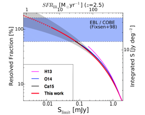
Figure 7.— Fraction of resolved EBL at 1.2 mm as a function of the detection limit, $S_{\rm limit}$. The red line and the gray shade indicate the best estimate from our study and the associated errors, respectively. The magenta, blue, and black lines present the estimates from the previous ALMA studies (hatsukade2013; ono2014; carniani2015). Here we re-calculate the resolved fractions of the previous studies with the bright source counts of scott2012. The blue shade denotes the IR EBL measurements from COBE (fixsen1998). The right axis represents the absolute values of the integrated flux densities, $\int^{\infty}_{S_{\rm limit}}S\phi(S)dS$, that correspond to the resolved EBL fraction. The top axis ticks IR star-formation rates $SFR_{\rm IR}$ corresponding to the 1.2 mm flux (kennicutt1998) for the case that a source resides at $z=2.5$.

With the best-fit Schechter parameter set, we calculate the integrated flux densities, $\int^{\infty}_{S_{\rm limit}}\it S\phi(S)dS$, down to the flux limit of $S_{\rm limit}$. Because the faintest bin of our number count data covers down to 0.015 mJy (Figure 6), we choose $S_{\rm limit}=0.015$ mJy. We calculate the integrated flux density to be $22.9^{+6.7}_{-5.6}$ Jy deg^-2 at 1.2 mm. Figure 7 shows the integrated flux density. We evaluate the fraction contributed to the total IR EBL measurement at 1.2 mm ($22^{+14}_{-8}$ Jy deg^-2; fixsen1998) that is obtained by the observations of the COBE Far Infrared Absolute Spectrophotometer (FIRAS), and find that the resolved fraction in our study is $104^{+31}_{-25}\%$. This result suggests that our study fully resolves the 1.2 mm EBL into the individual sources within the uncertainties.

Our result also indicates that the EBL contribution of sources with $\lesssim 0.02$ mJy are negligibly small. It would suggest that there is 1) a flattening of number counts slope $\alpha$, or 2) a truncation of the number counts at a flux $S_{\rm trunc}$ below $\simeq 0.02$ mJy. Using our resolved fraction of $f_{\rm res}=104^{+31}_{-25}\%$, we constrain $\alpha$ and $S_{\rm trunc}$ in the scenarios of 1) and 2). For the scenario of 1), we extrapolate the Schechter function from $S_{\rm limit}$ to 0 mJy with a power law of $n(S)\propto{S^{(\alpha_{\rm 0-S_{\rm limit}}}+1)}$, where $\alpha_{\rm 0-S_{\rm limit}}$ is a power law slope at $0$ mJy to $S_{\rm limit}$, and integrate the Schechter function with the power law extrapolation. We constrain the $\alpha_{0-S_{\rm limit}}$ value for the condition that the integrated flux density does not exceed the $1\sigma$ upper limit of the EBL measurement. We thus determine that the lower limit of $\alpha_{\rm 0-S_{\rm limit}}\gtrsim-1.0$. For the scenario of 2), we extrapolate our best-fit Schechter function below $S_{\rm limit}$. We find $S_{\rm trunc}\simeq 0.004$ mJy (corresponding to $SFR_{\rm IR}\sim 1.6$ $M_{\odot}{\rm yr^{-1}}$; kennicutt1998) where the $1\sigma$ lower error of $f_{\rm res}$ reaches 100% of the EBL contribution fraction. Because these 1) and 2) scenarios are two extreme cases, our results would suggest that the faint-end slope at $\lesssim 0.02$ mJy is flatter than the best-fit Schechter function slope of $\alpha=-2.12^{+0.07}_{-0.06}$ (Table 5), and that there is a number-counts truncation, if any, at $\lesssim 0.02$ mJy.

5. Clustering Analysis

5.1. Galaxy Bias of our Faint ALMA Sources

We estimate a galaxy bias of our faint ALMA sources by the counts-in-cells technique (e.g. adelberger1998; robertson2010)

$$b_{g}^{2}\approx\frac{\sigma_{N}^{2}-\bar{N}}{\bar{N}^{2}\sigma_{V}^{2}(z)},$$ (9)

where $\sigma_{N}^{2}$ is the standard deviation of the detected source counts per field, $\sigma_{V}^{2}$ is the matter variance averaged over the survey volumes $V$, and $\bar{N}$ is the average source counts per field.

In this counts-in-cells analysis, we use 66 maps of the field data (A) and (B). Because the cluster data (C) includes lensing effects of magnification and survey volume distortion as well as the different spurious source rate (Section 3.2), we do not include the cluster data (C) in the sample of our counts-in-cells analysis. The survey volume is calculated by using the average effective area per field (Section 3.6). For the redshift distribution to calculate the volume, we again assume a median redshift of $z=2.5$ (Section 3) and the top hat function covering $z=1-4$. For $\sigma_{N}^{2}$ and $\bar{N}$, we do not use the simple detection numbers, but the corrected detection numbers obtained with equation (5), which allows us to remove the effects of spurious sources. We calculate $\sigma_{V}^{2}$ with the analytic structure formation model (e.g., mo2002). To estimate the $1\sigma$ uncertainty of $b_{g}$, we carry out Monte-Carlo simulations. We first make 1000 mock catalogs of faint ALMA sources consisting of source counts that follow the Poission probability distribution function whose average values agree with our observed source counts. Then, we calculate galaxy bias values with each mock catalog, and repeat this process for the 1000 mock catalogs. We define a $1\sigma$ error of our observational $b_{g}$ estimate by the 68 percentile of the $b_{g}$ distribution obtained from the 1000 mock catalog results. Because the $1\sigma$ error is large, we cannot obtain the measurement of $b_{g}$ but place a $1\sigma$ upper limit of $b_{g}<3.5$ for our faint ALMA sources. This $1\sigma$ upper limit agrees with the previous $b_{g}$ estimate for faint ALMA sources, $b_{g}<4$, given by ono2014.

We estimate the dark halo masses of our faint ALMA sources with our result of $b_{g}<3.5$ with the analytics structure formation model of sheth1999, assuming the one-to-one correspondence between galaxies and dark halos. We obtain the $1\sigma$ upper limit dark halo mass of $\lesssim 5\times 10^{12}\ M_{\odot}$.

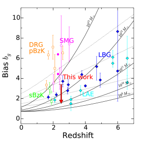
Figure 8.— Galaxy bias of our faint ALMA sources and the other high-$z$ galaxies. The red arrow shows the $1\sigma$ upper limit of our faint ALMA sources. The magenta arrows are the measurements and the upper limit for bright SMGs, which are calculated from the clustering results of webb2003; blain2004; weiss2009; williams2011; hickox2012. The orange and green squares denote the $K$-selected galaxies of DRGs/pBzK and sBzK, respectively (grazian2006; hayashi2007; quadri2007; blanc2008; furusawa2011; lin2012). The blue and cyan diamonds represent the UV-selected galaxies of LBGs (including BX/BM) and LAEs, respectively (ouchi2004; adelberger2005; overzier2006; lee2006; gawiser2007; ouchi2010). The solid curves indicate the galaxy biases of the dark halos with masses of $10^{9}$, $10^{10}$, $10^{11}$, $10^{12}$, and $10^{13}$ $M_{\odot}$ from bottom to top, which are predicted by the model of sheth1999 under the assumption of the one-to-one relation between galaxies and dark halos. The dotted curves present evolutionary tracks of dark halos for the galaxy conserving case, which assume that the motion of galaxy is purely caused by gravity with no galaxy merges (fry1996).

5.2. Comparison with Other Populations

Figure 8 shows the galaxy biases of our faint ALMA sources and a variety of high-$z$ galaxy populations; bright SMGs, $K$-selected galaxies including passively evolving BzK galaxies (pBzKs) and star-forming BzK galaxies (sBzKs), distant red galaxies (DRGs), and UV-selected galaxies composed of BX$/$BM galaxies, LBGs, and LAEs. Some of these high-$z$ galaxy studies shows no galaxy bias estimates, but only the galaxy correlation lengths $r_{0}$, and the power-law indices of the two point spatial correlation function $\gamma$. For these results, we calculate the galaxy biases in the same manner as ono2014 from $b_{g}=\sigma_{\rm 8,gal}/\sigma_{8}(z)$, where $\sigma_{8}(z)$ is a matter fluctuation in spheres of comoving radius of 8 $h^{-1}$Mpc, and $\sigma_{\rm 8,gal}$ is a galaxy fluctuation. The value of $\sigma_{\rm 8,gal}$ is derived with (see eq. 7.72 in peebles1993)

$$\sigma_{8,\rm gal}^{2}=\frac{72}{(3-\gamma)(4-\gamma)(6-\gamma)2^{\gamma}}\left(\frac{r_{0}}{8\ h^{-1}\rm{Mpc}}\right)^{\gamma}.$$ (10)

In Figure 8, the galaxy bias estimates for the most of SMGs, DRGs, and pBzKs are higher than the upper limit of our faint ALMA sources. On the other hand, $K$-selected star-forming galaxies of sBzKs have the halo masses comparable with those of our faint ALMA sources. The UV-selected LBGs and LAEs also have the galaxy bias values similar to our faint ALMA sources. Thus, we find that our faint ALMA sources are not similar to SMGs, DRGs, and pBzK with masses of $\gtrsim 10^{13}M_{\odot}$ but sBzKs, LBGs, and LAEs with masses $\lesssim 10^{13}M_{\odot}$ (Figure 8). These clustering results suggest a possibility in a statistical sense that a large fraction of our faint ALMA sources could be mm counterparts of sBzKs, LBGs, and LAEs.

6. Multi-Wavelength Properties of the Faint ALMA Sources

6.1. Optical-NIR Counterparts

We investigate optical-NIR counterparts of our faint ALMA sources, and characterize the sources with the multi-wavelength properties, especially the optical-NIR colors. We search for the optical-NIR counterparts in the regions of SXDS and A1689 that have rich multi-wavelength data. In these two regions, there are a total of 65 faint ALMA sources; 54 and 11 sources in SXDS and A1689 regions, respectively. For the optical-NIR counterpart studies so far conducted, this is the largest sample of faint mm sources down to $\sim 0.02$ mJy, while there exist studies, such as ALESS and COSMOS, that use a comparably large but relatively bright sample (hodge2013; scoville2015).

Table 6 summarizes the multi-wavelength data of SXDS and A1689 used in this study. The multi-wavelength data cover from X-ray to far-infrared (FIR) radiation. In the SXDS region, we use published photometry catalogs in 0.5-10 keV (ueda2008), $u^{*}$ (Foucaud et al. in preparation), $B$, $V$, $R$, $i^{\prime}$, $z^{\prime}$ (furusawa2008), $J$, $H$, $K$ (UKIDSS DR10; Almaini et al. in preparation), $3.6-24\ \mu$m (Spitzer UKIDSS Ultra Deep Survey; SpUDS), $250-500\ \mu$m (Herschel Multi-tiered Extragalactic Survey; HerMES, oliver2012), and 1.4 GHz (simpson2006) as well as the photometric redshift ($z_{\rm phot}$) catalog (williams2009). In the A1689 region, we investigate published photometry catalogs of $g_{475}$, $r_{625}$, $i_{775}$, $z_{850}$, $J_{110}$, $H_{160}$ (Hubble Source Catalog; HSC), $3.6-24\ \mu$m (Spitzer Enhanced Imaging Products; SEIP), $250-500\ \mu$m (HerMES), and the photometric redshift $z_{\rm photo}$ and spectroscopic redshift $z_{\rm spec}$ catalogs (limousin2007; coe2010; diego2015).

We use the $u^{*}$ to $K$ ($g^{\prime}$ to $H$) band images in the SXDS (A1689) region for the optical-NIR ($0.4-2\ \mu$m) counterpart identification, because these data have a good spatial resolution. The optical-NIR counterparts are defined by the criterion that the distance between optical-NIR and ALMA source centers is within a $1\farcs 0$. If an ALMA source meets this criterion in any of optical-NIR bands, we regard that the ALMA source has an optical-NIR counterpart. The $1\farcs 0$ radius is chosen, because the absolute positional accuracy (APA) of $\simeq 1\farcs 0$ is guaranteed in our ALMA data (cf. optical-NIR data for $\lesssim 0\farcs 3$; see, e.g., furusawa2008). Regarding the ALMA’s APA, the knowledge base page of ALMA Science portal presents that the APA is smaller than the synthesized beam width. Because the synthesized beam widths of our data are $\lesssim 1\farcs 0$, the $1\farcs 0$ radius is applied.

Using the SXDS+A1689 source catalog of the 65 faint ALMA sources, we identify a total of 17 optical-NIR counterparts. Fifteen and two sources are identified in SXDS and A1689 and referred to as S1-15 and A1-2, respectively. Figure LABEL:fig:postage_stamps shows the postage stamps of these identified sources, and Table 7 summarizes their photometric properties. The photometry values in Table 7 are total magnitudes. The $u^{*}$ magnitudes are MAG_AUTO values given by our SExtractor photometry. Similarly, $BVR_{c}i^{\prime}z^{\prime}$ magnitudes are MAG_AUTO values listed in the furusawa2008’s catalogs. The Spitzer photometry values are estimated from the SEIP aperture flux densities with the aperture correction , while the HST photometry values (for A1 and A2) are the total magnitudes calculated from MAG_APER values of our SExtractor measurements and the aperture correction . Note that there is an offset of $1\farcs 2$ ($1\farcs 06$) between the flux peaks of the optical-NIR counterpart and S9 (S15) ALMA source. Because S9 and S15 have an extended optical-NIR profile whose major component falls in the ALMA emitting region, the optical-NIR source is selected as a counterpart of the ALMA source.

Because spurious sources are included in the 65 faint ALMA sources, we calculate the real ALMA source number in the SXDS (A1689) region. In the SXDS (A1689) region, we subtract the expected spurious-source number of 31 (5) from the SXDS (A1689) source number of 54 (11), and estimate the real ALMA source number to be 23 (6). The total real ALMA source number in these two regions is 29 $(=23+6)$. Thus, the counterpart-identification fraction that is the ratio of the total optical-NIR counterpart ALMA sources to the real ALMA sources is estimated to be 59% (=17/29). We estimate the probability of the chance projection that a foreground or background object is located by chance in the $1\farcs 0$-radius circle of an ALMA source, and obtain $\sim 10\%$ in the $P$-value (downes1986). Multiplying this probability with the number of optical-NIR counterparts, 17, we expect that $\sim 2$ objects would be the foreground/background contamination. Even if we include this contamination effect, a half of our faint ALMA sources, 52% ($=[17-2]/29$), have an optical-NIR counterpart.

Interestingly, there is a difference of the counterpart-identification fractions between SXDS and A1689 regions, although the depths of the optical-NIR data are comparable in these two regions ($27-28$ mag in optical and $25-26$ mag in NIR; see Table 6). The counterpart-identification fraction in the SXDS region is 65% $(=15/23)$, while the one in the A1689 region is only 33% $(=2/6)$. Including the $1\sigma$ statistical uncertainties, these fractions are $65\pm 22$% and $33\pm 30$% for the SXDS and A1689 regions, respectively. We carefully examine whether this difference is just an artifact originated from, for examples, a systematically high spurious rate and cluster member galaxy obscurations in the cluster region. However, there are no hints of notable artificial effects in the data. chen2014 also report a similarly low-identification rate of MIR/radio counterparts in A1689 based on their observations with SMA. It should be noted that the intrinsic mm flux densities of our sources in the A1689 region are $\simeq 0.01-0.1$ mJy (magnification corrected) that is about an order of magnitude fainter than those of our sources in the SXDS region, $\simeq 0.1-1$ mJy.

There are two possible explanations for the difference between SXDS and A1689. The first explanation is made by the negative k-correction. Due to the faint flux densities, the mm sources of the A1689 would reside at a redshift higher than the SXDS sources on average, since the abundance of the dusty population decreases towards the epoch of the first-generation galaxies. Because the effect of the negative k-correction is significant, the ratio of mm to optical-NIR fluxes is higher for high-$z$ sources than low-$z$ sources. In this case, the counterpart-identification fraction would be small in the A1689 region. The second explanation is the A1689’s lensing distortion effects in conjunction with the intrinsic offsets between mm and optical-NIR emitting regions within a galaxy. chen2015 report that there is an offset between submm and optical-NIR emitting regions typically by $\sim 0\farcs 4$. If there is an intrinsic $\sim 0\farcs 4$ offset in the source plane of A1689, the image distortion effects of lensing would magnify the offset to $>1\farcs 0$. We thus estimate the probability that the offsets between mm and optical-NIR sources in the source plane is magnified to $>1\farcs 0$ in the image plane by Monte-Carlo simulations. We place 100 artificial sources in the source plane of A1689 at around an ALMA source in A1689. The positions of these artificial sources follow the Gaussian distributions whose standard deviation is $0\farcs 4$. Using our mass model, we calculate the offsets between the ALMA source and the artificial sources in the image plane. We repeat this process for 11 ALMA sources in A1689. We find that $\sim 50$% of the artificial sources show $>1\farcs 0$ offsets from the ALMA source in the image plane. Because the number of optical counterparts in A1689 is 2, our simulation results suggest that a total of 4 ($=2/[50\%]$) optical counterparts should exist in the case of no lensing distortion effects (+the intrinsic offsets). Thus, the true counterpart-identification fraction of A1689 is 67%($=4/6$) that is very similar to the counterpart-identification fraction of SXDS ($65\pm 22$%). If the lensing distortion effects (+the intrinsic offsets) would provide 2 ($=4-2$) sources whose optical counterparts have an offset from the ALMA sources by $>1\farcs 0$ in the image plane, we would find such ALMA sources whose optical counterparts are located at the position just beyond $1\farcs 0$ in our data. We refer the distribution of the artificial optical counterparts from our simulations, and search for potential optical-NIR counterparts whose distances from the ALMA sources are $>1\farcs 0$. We find such potential optical counterparts in 4 sources of A1689, some of which may be real optical counterparts, and confirm the hypothesis that the combination of the lensing distortion effects and the intrinsic offsets can be the major reason for the difference of the counterpart-identification fractions between the cluster of A1689 and the blank field of SXDS.

Table 7 lists the photometry of the Spitzer ($3.6-24\ \mu$m) and Herschel ($250-500\ \mu$m) data. Because the spatial resolutions of the Spitzer and Herschel data are poor, we determine the Spitzer and Herschel counterparts by visual inspection that allows sources residing at a position slightly beyond the $1^{\prime\prime}$ search radius. Although no sources are identified in the Herschel bands, about a half of our faint ALMA sources are detected in the Spitzer data. These results would indicate that our faint ALMA sources are very high redshift sources ($z>4$). However, it should be noted that the Herschel data can detect dusty starbursts whose SFRs are very high, $>$ a few $100M_{\odot}{\rm yr}^{-1}$ even at $z\sim 2-3$.

Here we examine whether we simply miss red spectral energy distribution (SED) objects that are not detected in optical-NIR ($0.4-2\ \mu$m) bands but only in Spitzer and Herschel bands. We search for Spitzer and Herschel counterparts of our faint ALMA sources with no optical-NIR counterparts, adopting the visual inspection technique described above. We find no Spitzer and Herschel counterparts that have undetectable optical-NIR fluxes. Again, these results do not suggest that our faint ALMA sources are dusty starbursts.

We cross-match the catalogs of our faint ALMA sources and the radio 1.4 GHz and X-ray 0.5-10 keV sources. We find no counterparts within a $1\farcs 0-3\farcs 0$ radius around our faint ALMA sources. Thus, our faint ALMA sources have no signatures of AGN.

To summarize these counterpart identification results with the Spitzer and Herschel as well as radio and X-ray data, there are signs of neither dusty starbursts nor AGNs in our faint ALMA sources. Note that these cross-match analysis is completed only in SXDS because there are no radio and X-ray data available in A1689.

Table 6Multi-wavelength Data

Region ($N_{counter}$)	Telescope/Instrument	Band (5$\sigma$ limit in mag)	Reference
(1)		(2)	(3)
SXDS (15)	XMM-Newton/EPICs, pn, MOS	0.5-10 keV ($6-50\times 10^{-16}$ erg cm-2 s-1)	(a)
	CFHT/MegaCam	$u^{*}(27.7)$	(b)
	Subaru/Suprime-Cam	$B$ (28.4)	(c)
	Subaru/Suprime-Cam	$V$ (28.0)	(c)
	Subaru/Suprime-Cam	$R_{c}$ (27.8)	(c)
	Subaru/Suprime-Cam	$i^{\prime}$ (27.7)	(c)
	Subaru/Suprime-Cam	$z^{\prime}$ (26.7)	(c)
	UKIRT/WFCAM	$J$ (25.6)	(d)
	UKIRT/WFCAM	$H$ (24.8)	(d)
	UKIRT/WFCAM	$K$ (25.4)	(d)
	Spitzer/IRAC	3.6$\mu$m (24.7)	(e)
	Spitzer/IRAC	4.5$\mu$m (24.6)	(e)
	Spitzer/IRAC	5.8$\mu$m (22.3)	(f)
	Spitzer/IRAC	8.0$\mu$m (22.3)	(f)
	Spitzer/MIPS	24$\mu$m (18.0)	(f)
	Herschel/SPIRE	250$\mu$m (13.8)	(g)
	Herschel/SPIRE	350$\mu$m (14.0)	(g)
	Herschel/SPIRE	500$\mu$m (13.6)	(g)
	VLA	1.4 GHz (20.0)	(h)
A1689 (2)	HST/ACS	$g_{475}$ (28.6)	(i)
	HST/ACS	$r_{625}$ (28.3)	(i)
	HST/ACS	$i_{775}$ (28.2)	(i)
	HST/ACS	$z_{850}$ (27.8)	(i)
	HST/NICMOS	$J_{110}$ (26.2)	(j)
	HST/WFC3	$H_{160}$ ($26.3-28.1$)	(k)
	Spitzer/IRAC	3.6$\mu$m (24.8)	(l)
	Spitzer/IRAC	4.5$\mu$m (24.3)	(l)
	Spitzer/IRAC	5.8$\mu$m (23.4)	(l)
	Spitzer/IRAC	8.0$\mu$m (22.9)	(l)
	Spitzer/MIPS	24$\mu$m (19.5)	(l)
	Herschel/SPIRE	250$\mu$m (14.0)	(g)
	Herschel/SPIRE	350$\mu$m (14.2)	(g)
	Herschel/SPIRE	500$\mu$m (13.8)	(g)

Note. — Columns: (1) Name of the region. The number, $N_{\rm counter}$, in the parenseses indicates the number of the optical-NIR counterparts. (2) Limiting magnitude defined by 5$\sigma$ sky noise in a circular aperture with a radius of PSF FWHM. (3) Reference or source catalogue: (a) ueda2008; (b) Foucaud et al. (in preparation); (c) furusawa2008; (d) UKIDSS (O. Almaini et al. in preparation); (e) SEDS (ashby2013); (f) SpUDS; (g) HerMES (oliver2012); (h) simpson2006; (i) Alavi et al. (2014); (j) bouwens2009; (k) bouwens2015; (l) SEIP.

Table 7Photometry of the Optical-NIR Counterparts

SXDS
ID	$u^{*}$	$B$	$V$	$R_{c}$	$i^{\prime}$	$z^{\prime}$	$J$	$H$	$K$	3.6$\mu$m	4.5$\mu$m	5.8$\mu$m	8.0$\mu$m	24$\mu$m	250$\mu$m	350$\mu$m	500$\mu$m
S1	$\cdots$	24.46	24.24	23.85	23.52	22.88	$\cdots$	$\cdots$	$\cdots$	20.02	19.94	20.11	20.12	$>18.56$	$>14.35$	$>14.55$	$>14.15$
S2	$\cdots$	25.91	26.18	26.59	26.71	25.01	$\cdots$	$\cdots$	$\cdots$	$>25.27$	$>25.16$	$>22.85$	$>22.81$	$>18.56$	$>14.35$	$>14.55$	$>14.15$
S3	27.24	26.69	26.35	25.63	25.29	25.25	24.80	24.43	24.41	$>25.27$	$>25.16$	$>22.85$	$>22.81$	$>18.56$	$>14.35$	$>14.55$	$>14.15$
S4	25.76	25.61	25.30	25.00	24.47	24.05	23.21	22.92	22.66	21.68	21.84	$>22.85$	$>22.81$	$>18.56$	$>14.35$	$>14.55$	$>14.15$
S5	26.31	25.11	24.70	24.76	24.58	24.75	24.53	24.05	24.22	$>25.27$	$>25.16$	$>22.85$	$>22.81$	$>18.56$	$>14.35$	$>14.55$	$>14.15$
S6	25.69	24.84	23.76	22.79	21.96	21.55	20.81	20.42	20.08	19.61	20.06	19.95	20.24	$>18.56$	$>14.35$	$>14.55$	$>14.15$
S7	$>28.23$	27.14	27.42	27.30	27.32	26.62	$>26.18$	$>25.31$	$>25.94$	$>25.27$	$>25.16$	$>22.85$	$>22.81$	$>18.56$	$>14.35$	$>14.55$	$>14.15$
S8	24.57	$>28.93$	$>28.56$	$>28.33$	$>28.24$	$>27.22$	$>26.18$	$>25.31$	$>25.94$	$>25.27$	$>25.16$	$>22.85$	$>22.81$	$>18.56$	$>14.35$	$>14.55$	$>14.15$
S9	$>28.23$	25.30	23.86	22.96	21.63	20.93	20.24	20.22	20.45	20.40	20.78	20.46	$>22.81$	$>18.56$	$>14.35$	$>14.55$	$>14.15$
S10	$>28.23$	26.68	26.25	26.25	25.65	25.07	25.90	24.60	25.67	$>25.27$	$>25.16$	$>22.85$	$>22.81$	$>18.56$	$>14.35$	$>14.55$	$>14.15$
S11	26.00	25.14	24.66	24.53	24.02	23.62	22.36	21.76	21.26	19.91	19.69	19.31	19.51	15.95	$>14.35$	$>14.55$	$>14.15$
S12	23.45	23.22	22.96	22.94	22.65	22.45	21.55	21.18	20.88	19.89	19.66	19.35	19.62	16.66	$>14.35$	$>14.55$	$>14.15$
S13	$>28.23$	$>28.93$	28.50	$>28.33$	$>28.24$	$>27.22$	$>26.18$	$>25.31$	25.22	22.55	22.73	22.33	$>22.81$	$>18.56$	$>14.35$	$>14.55$	$>14.15$
S14	$>28.23$	25.96	26.09	25.68	$>28.24$	$>27.22$	$>26.18$	$>25.31$	$>25.94$	$>25.27$	$>25.16$	$>22.85$	$>22.81$	$>18.56$	$>14.35$	$>14.55$	$>14.15$
S15	23.87	23.49	23.40	23.08	22.84	22.42	21.72	21.25	21.16	20.27	20.12	20.32	19.89	$>18.56$	$>14.35$	$>14.55$	$>14.15$
Abell 1689
ID	$\cdots$	$\cdots$	$g_{475}$	$r_{625}$	$i_{775}$	$z_{850}$	$J_{110}$	$H_{160}$	$\cdots$	3.6$\mu$m	4.5$\mu$m	5.8$\mu$m	8.0$\mu$m	24$\mu$m	250$\mu$m	350$\mu$m	500$\mu$m
A1	$\cdots$	$\cdots$	26.61	25.78	24.79	25.36	24.29	23.55	$\cdots$	18.25	18.45	18.72	19.10	16.94	$>14.55$	$>14.75$	$>14.35$
A2	$\cdots$	$\cdots$	27.35	26.28	25.84	25.59	$>26.75$	24.36	$\cdots$	$>25.35$	$>24.85$	$>23.95$	$>23.45$	$>20.05$	$>14.55$	$>14.75$	$>14.35$

Note. — The $u^{*}$ magnitudes are MAG_AUTO values given by our SExtractor photometry. Similarly, $BVR_{c}i^{\prime}z^{\prime}$ magnitudes are MAG_AUTO values listed in the furusawa2008’s catalogs. The Spitzer photometry values are total magnitudes estimated from the SEIP aperture flux densities with the aperture correction, while the HST photometry values (for A1 and A2) are the total magnitudes calculated from MAG_APER values of our SExtractor measurements. The aperture corrections for the Spitzer and HST photometry are provided by the Spitzer and HST websites, respectively (see text). The lower limits correspond to the $3\sigma$ levels. The S1 and S2 objects are not observed in $u^{*}$ band and $JHK$ bands.

6.2. Lensed ALMA Sources in A1689

We identify two optical counterparts of A1 and A2 that are lensed by the A1689 cluster. The optical image at the position of A1 is presented in Figure 9. There is a small positional offset of $\sim 0\farcs 8$ between the optical and mm emission, but this small difference can be explained by the positional uncertainty of the ALMA image (Section 6.1) .

This optical counterpart of A1 is one of three known multiple images that is dubbed 5.2, while the rest of two multiple images are called 5.1 and 5.3 (limousin2007). We investigate our ALMA image at the optical positions of 5.1 and 5.3 sources. In the ALMA image, the 5.1 source is marginally detected at the $3\sigma$ level, while the 5.3 source has no signals above the $3\sigma$ level. Table 8 summarizes the physical properties of these three multiple images. The difference of mm emissivities between these multiple images is discussed in Section 6.1.

Although the 5.2 source, i.e. A1, does not have a spectroscopic redshift, the redshift of the 5.1 and 5.3 sources is $z=2.60$ determined by spectroscopy (Richard et al. in preparation, see limousin2007). We thus regard that the redshift of A1 is $z=2.60$. We calculate the intrinsic 1.2 mm flux of A1 from our 1.3 mm data with the flux scaling factor from 1.3 mm to 1.2 mm (Section 3), and obtain $0.020\pm 0.008$ mJy that is corrected for the gravitational lensing magnification of $\mu=22.8$ and the primary beam sensitivity. chen2014 report that the 5.1 and 5.3 sources are not detected above the $3\sigma$ level by their Submillimeter Array (SMA) $870\ \mu$m observations, but only the 5.2 source. chen2014 measure the flux of the 5.2 source, and find the intrinsic flux of 5.2 source is 0.085 $\pm 0.035$ mJy at $870\ \mu$m, which corresponds to $0.033\pm 0.014$ mJy at 1.2 mm with the $k$-correction from $870\ \mu$m to 1.2 mm (Section 3). This 1.2 mm flux of $0.033\pm 0.014$ mJy is consistent with our measurement of $0.020\pm 0.008$ mJy within the 1$\sigma$ uncertainties.

The optical-NIR counterpart of A2 is identified in the optical bands with a lensing magnification factor of $\mu=4.9$. The intrinsic 1.2 mm flux of A2 is estimated to be $0.077\pm 0.035$ mJy that are corrected for the gravitational lensing magnification and the primary beam attenuation. Neither $z_{\rm spec}$ nor $z_{\rm photo}$ of A2 are available in the literature.

We compare these A1689 sources with optical-NIR counterparts (Table 8) and the previously-known lensed sources, Cosmic Eylash (e.g., swinbank2010) and SMMJ16358 (e.g., kneib2004), identified by single-dish observations. Cosmic Eyelash and SMMJ16358 have intrinsic SFRs of $\sim 210$ and $500M_{\odot}{\rm yr}^{-1}$, respectively. These SFRs correspond to $0.5$ and $1.3$ mJy at 1.2 mm under the assumption of the $SFR-L_{\rm IR}$ relation (kennicutt1998). On the other hand, our optical-NIR counterparts have intrinsic fluxes of $\sim 0.02-0.08$ mJy at 1.2 mm. Thus, our ALMA study has identified sources with intrinsic fluxes $\gtrsim 10$ times fainter than these lensed sources.

Although there are no optical-NIR counterparts, we find a very strongly lensed source candidate, A3, that shows ALMA flux double peaks dubbed A3a and A3b. The upper panel of Figure 10 shows the ALMA image of A3. The A3 source is very close to the critical line for a $z=3$ source (Figure 10), and the critical line is located between the double peaks of A3. More quantitatively, we investigate whether these double peaks can be explained by multiple images of a single lensed source behind A1689. Using our mass model, we calculate positions of multiple images made by a lensed source at $z=2-6$ (cyan lines in the upper panel of Figure 10). We find that multiple images at $z\sim 3$ reproduce the positions of the double peaks very well. The best-fit redshift is $z=3.07$, and the magnification factor is very high, $159$. The bottom panel of Figure 10 is the HST optical images. No optical counterparts of A3 are found. We summarize the properties of A3 in Table 9.

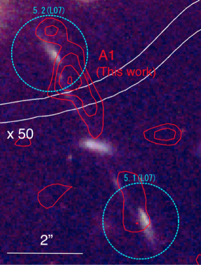
Figure 9.— False-color image of A1. The used images and color assignment are the same as Figure 1. The center of the cyan circles pinpoint the positions of the 5.1 and 5.2 sources, which are two of the multiple images of the galaxy at $z_{\rm spec}=2.60$ (limousin2007; coe2010). The radius of the cyan circle is $1\farcs 0$ that corresponds to the search radius for the counterpart identifications. The red contours show the ALMA 1.3 mm emission at the 2, 3, 4, and 5 $\sigma$ levels. The white curves represent the lines for the lensing magnification of $\mu=50$.

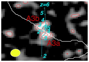
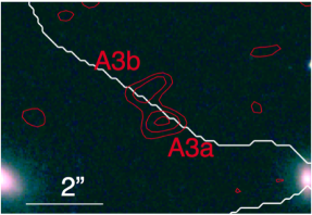
Figure 10.— Very strongly lensed source candidate, A3, found in A1689. The red contours show the ALMA 1.3 mm emission at the 2, 3, 4 $\sigma$ levels. The white curves denote the critical lines for a $z=3$ source that are estimated with our mass model. Top: ALMA continuum image of A3. The cyan tracks show the positions of multiple images for lensed sources at $z=2,3,4,5,$ and 6 that are predicted with our mass model. The ALMA multiple image positions (red contours; A3a and A3b) are well reproduced by a lensed source at $z\sim 3$. Bottom: False-color image of HST optical data showing the same region as the top panel. The used images and color assignment are the same as Figure 1. No optical counterparts of A3 are identified.

Table 8Multiple Images at $z=2.60$ with the ALMA Counterpart

ID	ID	R.A.	Decl.	$S_{\rm 1.3mm}^{\rm obs}$	$S_{\rm 1.3mm}^{\rm corr}$	$S_{\rm 1.2mm}^{\rm corr}$	$g_{475}$	$r_{625}$	$i_{775}$	$z_{850}$	$\mu$
(L07)	(This work)	(J2000)	(J2000)	(mJy)	(mJy)	(mJy)	(magAB)
(1)	(2)	(3)		(4)	(5)	(6)	(7)				(8)
5.1	$\cdots$	13:11:29.064	$-$1:20:48.64	0.18 $\pm$ 0.06	0.049 $\pm$ 0.021	0.067 $\pm$ 0.029	26.29	25.53	25.37	25.17	5.7
5.2	A1	13:11:29.224	$-$1:20:44.24	0.30 $\pm$ 0.06	0.015 $\pm$ 0.006	0.020 $\pm$ 0.008	26.61	25.78	25.58	25.36	22.8
5.3	$\cdots$	13:11:34.120	$-$1:20:20.96	$<$ 0.28	$<$ 0.093	$<$ 0.13	26.61	25.85	25.85	25.60	3.0

Note. — (1) and (2) ID names given in limousin2007 (L07) and this work, respectively. (3) R.A. and Decl. in the optical data. (4) Peak flux density SExtractor measurement (Section 3.1) with the primary beam correction. If no significant $1.32$ mm fluxes are detected at the optical source positions, three sigma upper limits are presented. (5) Observed flux density at 1.32 mm on the uv-taper image that are measured by 2D Gaussian-fitting routine of $imfit$ in CASA with the primary beam correction. The magnification uncertainty (Section 3.5) is included in the error. (6) Source flux density at 1.2 mm with the flux scaling from 1.32 mm to 1.2 mm (Section 3). (7) Total magnitudes in the HST/ACS bands. (8) Magnification factor at the peak of the optical flux.

Table 9Very Strongly Lensed Source Candidate

ID	R.A	Decl.	$S_{\rm 1.3mm}^{\rm obs}$	$S_{\rm 1.3mm}^{corr}$	$S_{\rm 1.2mm}^{corr}$	$g_{475}$	$r_{625}$	$i_{775}$	$z_{850}$	$\mu$
	(J2000)	(J2000)	(mJy)	(mJy)	(mJy)	(magAB)
(1)	(2)		(3)	(4)	(5)	(6)				(7)
A3	13:11:26.897	$-$1:20:32.02	0.24$\pm$0.06	$0.0015\pm 0.0007$	$0.0020\pm 0.0010$	$>28.56$	$>28.33$	$>28.24$	$>27.22$	159.5

Note. — (1) $-$ (7) correspond to (2) $-$ (8) in Table 8. These values are for the A3a component (Figure 10). Because A3a and A3b are confused in the uv-taper image, these fluxes are obtained on the image without uv-taper.

6.3. Color and Luminosity Properties of the Optical-NIR Counterparts

We investigate color (i.e. SED) and luminosity properties of the optical-NIR counterparts, S1-15 and A1-2, to understand the population of the faint ALMA sources with the detectable optical-NIR continuum emission. First of all, we refer the catalog of photo-$z$ estimated from the optical-NIR SEDs (williams2009), and find that S11, S12, S15 have photo-$z$ values of $1.54^{+0.08}_{-0.02}$, $1.57^{+0.07}_{-0.02}$, and $1.45^{+0.03}_{-0.02}$, respectively. However, the photo-$z$ values of the S4 and S6 sources are $0.77^{+0.23}_{-0.03}$ and $0.67^{+0.01}_{-0.02}$, respectively. We thus regard that the S4 and S6 sources reside at low redshift ($z<1$), and find that $\sim 10$% $(=2/17)$ optical-NIR counterparts are low-$z$ objects. Because the majority of mm sources are thought to be high-$z$ galaxies and AGNs (casey2014), the rest of 15 ($=17-2$) optical-NIR counterparts are candidates of high-$z$ galaxies. We thus compare colors and luminosities of these high-$z$ galaxy candidates with those of high-$z$ sources. The major high-$z$ populations are SMGs, LBGs (including BX/BM), DRGs, BzKs, LAEs, and AGNs. Since the SMGs, DRGs, and LAEs generally have weak optical continua that cannot be reliably compared with our optical-NIR counterparts, we focus on the comparisons with LBGs (BX/BM) and BzKs.

6.3.1 Comparison with the LBG BX/BM Populations

The BX and BM galaxies, generally included in the LBG population, reside in the redshift ranges of $2.0\lesssim z\lesssim 2.5$ and $1.5\lesssim z\lesssim 2.0$, respectively (steidel2004). Similarly, there are LBGs at $z\sim 3$. These galaxies are defined by the selection criteria of $U_{n}-G$ and $G-R$ colors. We apply these color selection criteria to our optical-NIR counterparts, but the photometry bands of our data are different from the $U_{n}$, $G$ and $R$ bands. Following the procedures of ly2011, we alternatively use a color set of $U-BV$ and $BV-R_{c}i^{\prime}$. The $BV$ and $R_{c}i^{\prime}$ photometry are defined by

$$BV=-2.5{\rm log}\left[\frac{x_{1}f_{B}+(1-x_{1}f_{V})}{3630\ \mu Jy}\right],$$

$$R_{c}i^{\prime}=-2.5{\rm log}\left[\frac{x_{2}f_{R}+(1-x_{2}f_{i^{\prime}})}{3630\ \mu Jy}\right],$$ (11)

where $f_{X}$ is the flux density per unit frequency (erg s^-1 cm^-2 Hz^-1) in a band ’X’ corresponding to $B$, $V$, $R_{c}$, and $i^{\prime}$. The coefficients of $x_{1}$ and $x_{2}$ are $0.314$ and $0.207$, respectively. With these photometric relations and the selection colors (steidel2004), the color criteria of BX objects are re-written as

$$BV -R_{c}i^{\prime}\ \geq\ -0.2,$$ (12)

$$U -BV\ \geq\ BV-R_{c}i^{\prime}+0.23,$$

$$BV -R_{c}i^{\prime}\ \leq\ 0.2(u-BV)+0.4,$$

$$U -BV\ \leq\ BV-R_{c}i^{\prime}+1.0.$$

Similarly, the criteria of BM objects are

$$BV -R_{c}i^{\prime}\ \geq\ -0.2,$$ (13)

$$U -BV\ \geq\ -0.1,$$

$$BV -R_{c}i^{\prime}\ \leq\ -0.382(U-BV)+0.853,$$

$$BV -R_{c}i^{\prime}\ \leq\ 0.70(U-BV)+0.280,\$$

$$U -BV\ \geq\ BV-R_{c}i^{\prime}+0.23.$$

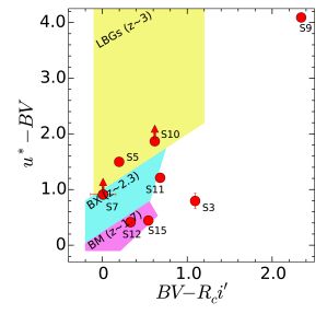
Figure 11.— Two-color diagram for our optical-NIR counterparts. The cyan and magenta-shaded regions are the BX and BM selection windows that are defined in the $BV-R_{c}i^{\prime}$ and $u^{*}-BV$ color plane (ly2011). The BX and BM galaxies reside at $z\simeq 2-2.5$ and $z\simeq 1.5-2.0$, respectively. The yellow shades indicate the approximate region of the selection window for $z\sim 3$ LBGs (steidel2003), where we assume that the original photometry of $U_{n}$, $G$ and $R$ bands are roughly the same as those of our $u^{*}$, $B$, and $R_{c}$ bands, respectively.

We compare these color criteria with our optical-NIR counterparts. Among the 17 optical-NIR counterparts, 10 are observed with the photometric system of $u^{*}BVR_{c}i^{\prime}$ necessary for the comparison. Removing the 2 obvious low-$z$ objects of S4 and S6, we use 8 optical-NIR counterparts. Figure 11 displays the two color diagram of these 8 sources with the color selection criteria. Six sources fall in or near the selection windows of $z\sim 2$ BX/BM or $z\sim 3$ LBGs, where we include S11 source at the border of the selection window. The S9 source is placed at the upper right corner of Figure 11. These colors of the S9 source are similar to $z\gtrsim 4$ LBGs (see, e.g., steidel2003). It is likely that S9 source is a LBG at $z\gtrsim 4$. On the other hand, S3 clearly escapes from the selection windows. We thus find that 7 out of 8 optical-NIR counterparts are have colors consistent with either $z\sim 2$ BX/BM or $z\gtrsim 3$ LBGs. Including the two low-$z$ objects of S4 and S6 sources, 70% $(=7/[8+2])$ of the optical-NIR counterparts meet the LBG (BX/BM) color criteria. We then compare magnitudes of the 10 optical-NIR counterparts with the known $z\sim 2$ BX/BM and $z\gtrsim 3$ LBGs, omitting $u^{*}$ magnitudes that would include a Lyman break whose central wavelength is very sensitive to a source redshift. We find that all of the 10 optical-NIR sources have $R_{c}$ magnitudes in the range of $23-27$ mag (Table 7) that is typical brightness of $z\sim 2$ BX/BM and $z\gtrsim 3$ LBGs (steidel2003; steidel2004). We thus conclude that a majority ($\sim 70$%) of the 10 optical-NIR counterparts belong to LBG (BX/BM) population.

6.3.2 Comparison with the BzK Populations

In contrast with BX/BM galaxies and LBGs, the BzK galaxy population includes not only blue star-forming galaxies, but also moderately reddened dust-poor star-forming galaxies (a.k.a sBzK) and passive galaxies (a.k.a pBzK) at $1.4\lesssim z\lesssim 2.5$ (daddi2004). We compare the color criteria of the BzK population with our optical-NIR counterparts. There are 10 out of the 17 optical-NIR counterparts that are located in the SXDS region with the photometric measurements of $B$, $z^{\prime}$, and $K$ bands (Table 7). Removing the 2 obvious low-$z$ objects of S4 and S6, we use 8 optical-NIR counterparts for the comparison.

Because the photometry system of ours (SXDS) is different from that of the BzK studies (daddi2004), we again apply corrections to the color selection criteria for BzK galaxies, which are suggested by yuma2012,

$$(B-z)_{\rm Daddi+04}=(B-z)_{\rm SXDS}+0.3,$$

$$(z-K)_{\rm Daddi+04}=(z-K)_{\rm SXDS}+0.1.$$ (14)

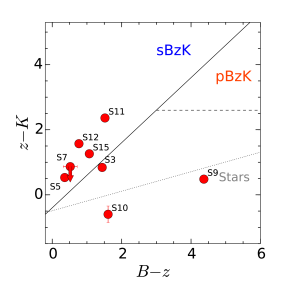
Figure 12.— Two-color diagram of the BzK galaxy selection in the SXDS photometry system The red circles denote the 7 optical-NIR counterparts. Star-forming galaxies at $z\simeq 1.4-2.5$, called sBzK galaxies, are selected in the region beyond the solid line defined by $(z-K)-(B-z)\ \geq\ -0.2$. The pBzK galaxies, passively evolving galaxies at $z\simeq 1.4-2.5$, are selected in the triangular region defined with the sold and dashed ($z-K>2.5$) lines at the upper right corner. Galactic stars fall in the region below the dotted line (See also daddi2004; yuma2012).

Figure 12 presents the $B-z$ and $z-K$ colors of the 8 optical-NIR counterparts. We find that 5 out of the 8 optical-NIR counterparts meet the color criteria of sBzK, while the rest of the three sources, S3, S9 and S10, have colors different from sBzK or pBzK galaxies whose redshift range is $z\simeq 1.4-2.5$. Because S3 also shows the colors different from those of BX/BM galaxies and LBGs (Section 6.3.1), S3 would reside at $z\lesssim 1.4$ that is out of the BzK redshift window. Although the colors of S9 and S10 are similar to those of stars, in Section 6.3.1, the BX/BM galaxy and LBG selections suggest these two sources have colors consistent with $z\gtrsim 3$ galaxies. Thus, S9 and S10 would be galaxies at $z\gtrsim 3$ that escape from the BzK redshift window. In this way, we confirm that the results of the BzK selection are consistent with those of BX/BM galaxies and LBGs. In summary, including the two low-$z$ objects of S4 and S6 sources, we find that $50\%$(=5/[8+2]) of the optical-NIR counterparts are sBzK galaxies at $z\simeq 1.4-2.5$. We then compare magnitudes of these optical-NIR counterparts (Table 7), and find that the optical and NIR magnitudes are comparable with the sBzK galaxies (daddi2004).

6.3.3 Comparison with the AGN Population

Six counterparts of S1, S6, S11, S12, S15, and A1 are detected in the mid IR of $8$ and $24\ \mu$m bands. Because mid-IR bright objects are prominent candidates of AGN that have strong hot-dust emission, we compare colors of the six mid-IR bright counterparts and a typical AGN (Mrk 231) as well as a starburst (Arp 220). Figure 13 shows the colors of the five mid-IR bright counterparts, Mrk 231, and Arp 220 in the diagnostic color diagram of $S_{8.0\mu\rm m}$/$S_{4.5\mu\rm m}$ vs. $S_{24\mu\rm m}$/$S_{8.0\mu\rm m}$ that separates AGN and starburst (SB) populations (ivison2004). In Figure 13, the dashed and dotted lines indicate the color tracks of Mrk 231 and Arp 220 in the redshift range of $0.5-3.0$ that is taken from Figure 4 of ivison2004. All of our five mid-IR bright counterparts are placed near the color track of Arp 220, and far from the one of Mrk 231, which suggest that these six counterparts are not AGN but starbursts.

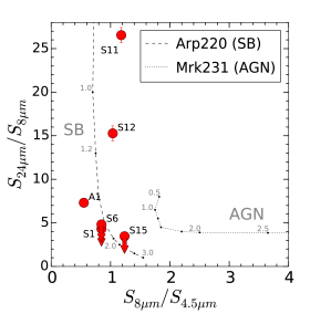
Figure 13.— Color-color diagram for the AGN diagnostics. The red circles and upper limits are our five mid-IR bright counterparts. The dotted and dashed lines present the color tracks of Mrk 231 (AGN) and Arp 220 (SB), respectively, that are redshifted from $z\simeq 0.5$ to $3.0$. The numbers labeled to the lines represent the redshifts.

Table 10Properties of our Optical-NIR Counterparts

ID	R.A.	Decl.	$\lambda_{\rm obs}$	$S^{\rm obs}_{\lambda_{\rm obs}}$	$S^{\rm corr}_{\rm 1.2mm}$	$z_{\rm photo}$	$z_{\rm spec}$	sBzK	pBzK	BX$/$BM$+$LBG	AGN
	(J2000)	(J2000)	(mm)	(mJy)	(mJy)
			(1)	(2)	(3)	(4)	(5)	(6)	(7)	(8)	(9)
S1	34.612686	$-$4.583063	1.22	0.36 $\pm$ 0.07	0.43 $\pm$ 0.09	$\cdots$	$\cdots$	$\cdots$	$\cdots$	$\cdots$	N
S2	34.613739	$-$4.588505	1.22	0.31 $\pm$ 0.09	0.31 $\pm$ 0.10	$\cdots$	$\cdots$	$\cdots$	$\cdots$	$\cdots$	$\cdots$
S3	34.437805	$-$5.494339	1.03	0.056 $\pm$ 0.015	0.032 $\pm$ 0.010	$\cdots$	$\cdots$	N	N	N	$\cdots$
S4	34.446648	$-$5.007715	1.26	0.047 $\pm$ 0.014	0.044 $\pm$ 0.016	0.77${}^{+0.23}_{-0.03}$	$\cdots$	$\cdots$	$\cdots$	$\cdots$	$\cdots$
S5	34.446007	$-$5.008159	1.26	0.049 $\pm$ 0.014	0.050 $\pm$ 0.017	$\cdots$	$\cdots$	Y	N	Y	$\cdots$
S6	34.387825	$-$5.220457	1.25	0.41 $\pm$ 0.11	0.42 $\pm$ 0.13	$0.67^{+0.01}_{-0.02}$	$\cdots$	$\cdots$	$\cdots$	$\cdots$	N
S7	34.411190	$-$4.745051	1.23	0.30 $\pm$ 0.08