A DETAILED STUDY OF GIANTS AND HORIZONTAL BRANCH STARS IN M68: ATMOSPHERIC PARAMETERS AND CHEMICAL ABUNDANCES

Abstract

In this paper, we present a detailed high-resolution spectroscopic study of post main sequence stars in the Globular Cluster M68. Our sample, which covers a range of 4000 K in $T_{\rm eff}$, and 3.5 dex in log(g), is comprised of members from the red giant, red horizontal, and blue horizontal branch, making this the first high-resolution globular cluster study covering such a large evolutionary and parameter space. Initially, atmospheric parameters were determined using photometric as well as spectroscopic methods, both of which resulted in unphysical and unexpected $T_{\rm eff}$, log(g), $\xi_{\rm t}$, and [Fe/H] combinations. We therefore developed a hybrid approach that addresses most of these problems, and yields atmospheric parameters that agree well with other measurements in the literature. Furthermore, our derived stellar metallicities are consistent across all evolutionary stages, with $\langle$[Fe/H]$\rangle$ = $-$2.42 ($\sigma$ = 0.14) from 25 stars. Chemical abundances obtained using our methodology also agree with previous studies and bear all the hallmarks of globular clusters, such as a Na-O anti-correlation, constant Ca abundances, and mild $r$-process enrichment.

1 INTRODUCTION

Along with M15 and M92, M68 is one of the lowest metallicity Galactic globular clusters (GC), [Fe/H] $\sim~{}$-2.3 Harris (1996). It has therefore been included in many large-sample light-element abundance studies (e.g., Bellazzini et al. 2012), but has thus far been subjected to very few detailed chemical composition investigations. In an analysis of red horizontal branch (RHB) stars in the metal-poor GC M15, Preston et al. (2006) found a declining difference between surface gravities determined from photometry and LTE spectrum analysis with increasing effective temperature in the range 5300 K < $T_{\rm eff}$ < 6300 K, a temperature range which embraces almost the entire RHB of that cluster. Contemporaneously, Lee et al. (2005, hereafter Lee05) found larger differences in surface gravities among the cooler ($T_{\rm eff}$$\ \sim$ 4200 K) red giant branch (RGB) stars of M68. In combination, these results suggest that non-LTE (NLTE) over-ionization of neutral metals produces systematic errors in abundance analyses of cool, metal-poor red giants in globular clusters, and that abundances derived from RHB stars may provide a more accurate abundance scale for metal-poor stars of globular clusters and the Galactic halo.

We decided to pursue this possibility by conducting an expanded investigation of post main sequence stars in M68, similar to that for M15 reported by Sobeck et al. (2011, hereafter Sob11). From a purely observational point of view, M68 has many advantages over M15. First, the RR Lyrae stars in M68 are $\ \sim$0.2 mag. brighter than those in M15 (Walker (1994, hereafter Wal94)). Second, all of our observations were done at the Las Campanas Observatory (LCO), and since M68 has $\delta$ = $-$27°, it transits the meridian near the zenith, whereas M15, with $\delta$ = +12°, lies low in LCO’s northern sky. See Table 1 for more fundamental parameters of M68.

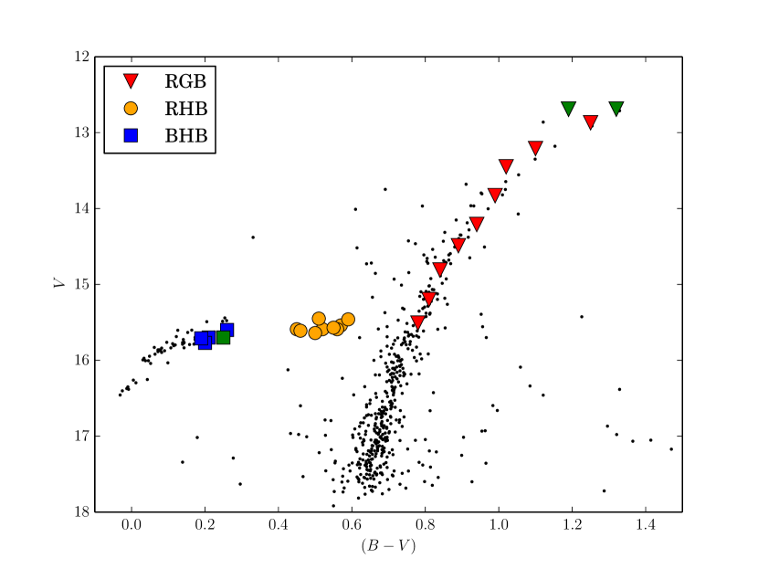
Figure 2: CMD of M68 using Walker (1994) data. The markers and colors defined here for the RGB, RHB, and BHB will be used throughout the remaining plots in this paper. The green points represent non-standard stars. Please see §4.5 for more details.

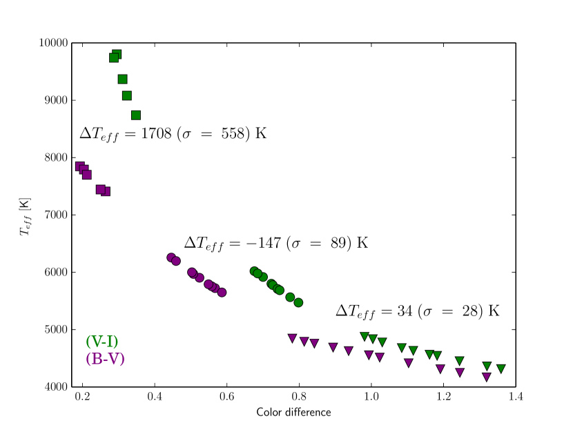
Figure 3: Here we show the implied $T_{\rm eff}$ values for each of the color indices. For the purposes of this figure, $\Delta\mbox{$T_{\rm eff}$}\equiv\mbox{$T_{\rm eff}$}_{(V-I)}-\mbox{$T_{\rm eff}$}_{(B-V)}$. As before, RGBs are represented as triangles, RHBs as circles, and BHBs as squares.

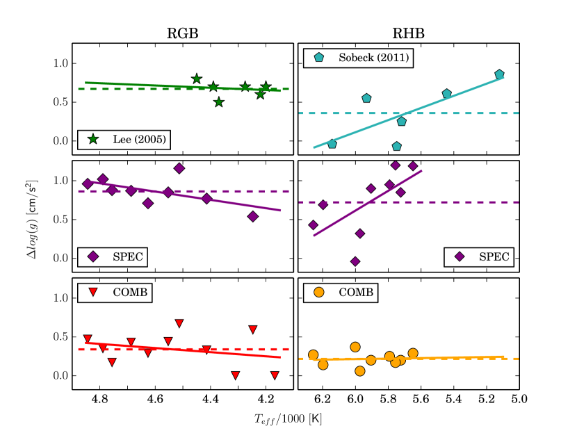
Figure 5: Comparisons of $\Delta\mbox{log({\it g})}\ (\equiv\mbox{log({\it g})}_{PHOT}-\mbox{log({\it g})}_{comparison\ value})$ values as a function of temperature for different studies and methodologies. The solid lines represent a linear fit to the data, while dashed lines give the average $\Delta\mbox{log({\it g})}$ offset.

In addition to being more accessible observationally, M68 differs from M15 in several other important respects. M68 has a relatively sparsely populated RHB compared to M15, which possesses an extended blue horizontal branch (EHB) (Durrell & Harris 1993). This is also reflected in the horizontal branch ratio, defined to be the ratio of horizontal branch stars to red giant stars, for both clusters. For M15, this ratio is 0.67, while for M68 it’s only 0.17 (Zinn 1986, Harris 1996). Such differences in HB morphology have been studied extensively (e.g. Lee et al. 1994 and Caputo et al. 1980) and attributed to variations in cluster age and metallicity, as well as stellar helium abundances and rotation (see Figs. 2-5 in Lee et al. 1994). Since M15 and M68 have very similar ages and metallicities, the differences in HB morphology could be attributed to disparate He contents.

M68 and M15 also seem to exhibit systematically different abundance patterns. Lee05 found $\langle\mathrm{[Si/Fe]\rangle_{M68}}\sim 0.6$, while $\langle\mathrm{[Si/Fe]}\rangle_{\mathrm{M15}}\sim$ 0.2 (Sob11). Si abundances in ‘normal’ Pop II stars are equivalent to those of M68 RGBs (Lee05, Cayrel et al. 2004). Furthermore, M68 seems underabundant in Ti (Lee05), whereas overabundances of neutron capture elements, which vary from star to star, are found in the RHB and RGB stars of M15. Finally, M15 contains dusty red giants (Boyer et al. (2006)), surprising in view of the low metallicity, and interesting as unusually large mass loss during post main sequence evolution has been advanced as an explanation for the EHB (D’Cruz et al. 1996).

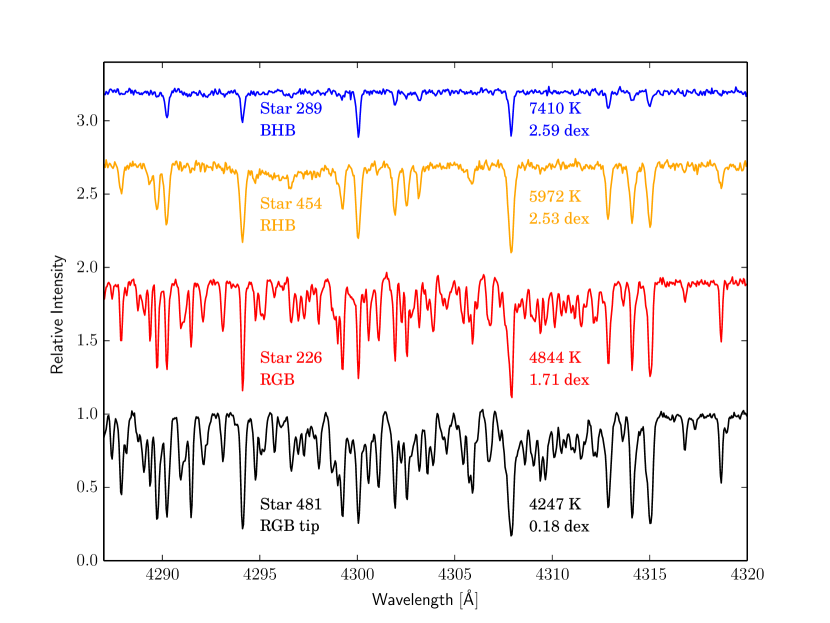
Figure 1: Sample spectra for all evolutionary stages in our sample. In addition to the name and evolutionary state of the star, we also list $T_{\rm eff}$ and log(g). This specific wavelength region covers the CH G-band. Measuring this band in the RHB and BHB is nearly impossible due to their higher $T_{\rm eff}$ and log(g) values.

In this paper, we derive atmospheric parameters in a self-consistent fashion for RGB, RHB, and blue horizontal branch (BHB) stars in M68, which span about 4000 K in $T_{\rm eff}$ and 3.5 dex in log(g). Figure 1, which shows a small spectral region for all evolutionary stages in our sample, highlights the difficulties of a self-consistent analysis over such a large parameter space. Several challenges, such as the breakdown of photometric temperature calibrations, as well as the unphysicality of certain spectroscopic methodology assumptions, have to be overcome. After exploring photometric and spectroscopic methods to determine the values of $T_{\rm eff}$, log(g), $\xi_{\rm t}$, and [Fe/H], we develop a hybrid atmospheric analysis strategy that appears to yield reasonable parameters for the RGB, RHB, and BHB stars. Using these parameters, we present a detailed abundance analysis, which will allow us to gain insight about the chemical evolution of M68.

2 OBSERVATIONS AND REDUCTIONS

We obtained high resolution spectra of 11 red giant branch, 9 red horizontal branch, and 5 blue horizontal branch members of M68. All of our program stars were selected from the photometric survey of Wal94, whose $V$ and $B-V$ values are listed in in Table 2. Figure 2 shows the Walker color-magnitude diagram for M68, using symbol shapes and colors to distinguish the RGB, RHB, and BHB stars observed in this study. The observed RGB members were selected to represent stars from the giant branch tip down to the luminosity of the horizontal branch, while RHB candidates were chosen to cover most of their evolutionary stage up to the red edge of the RR Lyr gap ($B-V$ $\simeq$ 0.45). BHB candidates were chosen to be between the blue RR Lyr edge ($B-V$ $\simeq$ 0.25) and the $T_{\rm eff}$ domain ($B-V$ $\gtrsim$ 0.2) in which stellar atmospheric effects begin to distort the observed chemical compositions of stars (eg., Khalack et al. 2010, Behr 2003 and references therein). Although M68 has more than 40 known RR Lyr stars (e.g., Castellani et al. 2003 and references therein), none of these were included in our study since spectrograph integration times would have been too long to acquire adequate data for these rapidly changing stars.

Our spectra were gathered with the Magellan Inamori Kyocera Echelle (MIKE) spectrograph (Bernstein et al., 2003) of the LCO Magellan Clay 6.5 m telescope. The spectrograph was configured with a 0.7$\arcsec$ entrance aperture that yielded an ultimate resolving power of $R\equiv\lambda/\Delta\lambda$ $\sim$ 40,000 for both the blue and red arms of instrument. The useful spectral coverage of the blue arm was 3500$-$5000 Å, and that of the red arm was 5000$-$9000 Å. Scattered light and sky subtraction, as well as cosmic-ray filtering and flat field division were performed with software developed by S.A. Shectman (2004, unpublished). Wavelength calibrations were based on co-added hollow cathode Th-Ar spectra, obtained before and after each observation. Other one-dimensional extractions were completed using the apall package of IRAF.

3 LINE LISTS AND EQUIVALENT WIDTHS

3.1 Atomic Line List

Table 3 lists the lines of atomic species and their associated log(gf) values employed in this work. Measured equivalent width ($EW$) values, as well as the sources of our $gf$-values can be found in last column of this table. We call attention to Fe II, for which Meléndez & Barbuy (2009) have proposed a renormalization of its transition probabilities based on some laboratory $gf$’s and an inverted solar spectrum analysis. These renormalized $gf$ values are in general about 0.1 dex lower than those in the NIST Atomic Spectra Database, which were employed by us. If we had adopted the Meléndez & Barbuy results here, our Fe II-based abundances would be larger by about 0.1 dex, which, in turn, would have decreased derived gravities by about 0.2 dex. We will return to this point later.

3.2 Equivalent Width Measurements

The equivalent width (EW) measurements were done in a semi-automated manner using an IDL code (EW.pro) initially described in Roederer et al. (2010) and further developed by Brugamyer et al. (2011). This code allows the user to visually inspect either a Gaussian or Voigt $\chi^{2}$ minimization fit for each line, ensuring that any obviously blended or any otherwise undesirable line will not be measured. Additionally, the user can adjust the continuum which reduces any error possibly introduced by faulty normalization of the spectra. Several lines were picked out at random from all stars and re-measured using the SPECTRE code (Fitzpatrick & Sneden, 1987). Four members of our sample (RGB stars 256, 472 and RHB stars 403, 458) were analyzed entirely using SPECTRE. The EWs obtained in this fashion were then compared to those derived using the IDL code. On average, the difference between the EW values derived using EW.pro and those derived using SPECTRE are $\Delta_{EW}=-1.18\ (\sigma$ = 3.18) mÅ. We therefore regard the differences in measured EW as negligible.

The S/N, which is a function of wavelength and $T_{\rm eff}$ of our programs stars, directly influenced the EW limitations for lines used in our analysis. A set of final S/N estimates for all of our stars can be found in Table 4. All S/N values given in this Table were estimated using the no routine of SPECTRE at around 6600 Å in each star. For most stars, the lower EW cutoff was $\sim$ 10 mÅ, while the upper limit was set at $\sim$ 150 mÅ, depending on evolutionary state and line species. These limits, especially the lower cutoff, were not applied to star 334, as its S/N is about 70% lower than the average of our sample. For this star, any line that could be measured with a healthy degree of certainty, except the obviously saturated ones, was used.

4 MODEL ATMOSPHERIC PARAMETERS

4.1 Initial Parameters

General information about M68, relevant to determining atmospheric parameters of our stars, can be found in Table 1. Special attention is called to the assumed distance modulus, $(m-M)_{V}$, and the reddening, $E(B-V)$, as they are of importance in determining photometric $T_{\rm eff}$ and log(g) values.

Initial atmospheric parameters were determined from BVI photometry obtained by Wal94 (see Table 2). To convert the given fluxes to $T_{\rm eff}$ values, the (B-V) and (V-$I_{C}$) IRFM (infrared flux method) calibrations of Ramírez & Meléndez (2005) were used. Although there is a more recent calibration available (Casagrande et al. 2010), only Ramírez & Meléndez (2005) include a calibration for giant stars. Figure 3 compares the $T_{\rm eff}$ values obtained from (B-V) and (V-$I_{C}$) colors. In the RGB, these two indices give approximately the same answer, while they start to diverge in the RHB and BHB. This behavior can be explained by the lack of calibration stars at (V-$I_{C}$) $<$ 0.6. Additionally, the difference between the V and $I_{C}$ fluxes becomes insensitive to changes in temperature at (V-$I_{C}$) $<$ 0.65, since the bandpasses of the respective filters are now in the temperature insensitive tail of the blackbody distribution. For these reasons, we chose (B-V) to be the sole color index in determining photometric temperatures.

Initial surface gravity values were derived using the standard formula:

$$\mbox{log({\it g})}_{\star}=0.4(M_{\rm V\star}+BC-M_{\rm Bol\sun})+\mbox{log({\it g})}_{\sun}+4{\rm log}\left(\frac{\mbox{$T_{\rm eff}$}_{\star}}{\mbox{$T_{\rm eff}$}_{\sun}}\right)+{\rm log}\left(\frac{{\it M}_{\star}}{{\it M}_{\sun}}\right).$$

For the solar values, $\ M_{\rm Bol\sun}$ = 4.75, $T_{\rm eff}$_☉ = 5777 K, and log(g)_☉ = 4.44 km s^-1 were assumed. The assumed stellar mass in the above equation was estimated to be $M_{\star}\approx$ 0.7$\ M_{\sun}$, a result obtained from a isochrone calculation with M68 metallicity and age values (see §4.5 for more details). Since $\mbox{log({\it g})}_{\star}$ varies linearly with log($M_{\star}$), an accurate value of stellar mass was not needed in this calculation. The bolometric correction (BC) for each star was calculated from the calibration given in Alonso et al. (1999). This calibration, however, does not hold for stars with $T_{\rm eff}$$\ \geq$ 6300 K. For stars exceeding this temperature, Figure 3 of Flower (1996) was used to obtain an estimate of the stellar BC. $T_{\rm eff}$ and log(g) values obtained in this fashion will be referred to as PHOT in texts and figures throughout the rest of this paper.

Initial microturbulent velocities ($\xi_{\rm t}$) were estimated to be 1.2 km s^-1 for all RGB stars in our sample. For RHB stars, calibrations provided in Gratton et al. (1996) were used. Initial BHB $\xi_{\rm t}$ estimates were obtained by calculating a temperature dependent linear fit of a previous BHB study (For & Sneden 2010), and applying the resulting calibration to our stars. Lastly, an initial atmospheric metallicity of [Fe/H] = $-$2.23 (from the 2010 edition of Harris 1996) was assumed.

4.2 Final Parameters

We employed three different methodologies to converge on our final set of parameters. In addition of the purely photometric PHOT parameter set defined above, we also derived purely spectroscopic parameters. These will be referred to as SPEC. Our final adopted set of parameters, which are a combination of photometry and spectroscopy, are called COMB. These designations will be used throughout the rest of this paper, including all plots. Abundances for the various approaches were calculated using the latest version of MOOG (Sneden 1973), except in the case of the RGB stars. In their temperature/gravity/metallicity regime, the major electron donors for the $H^{-}$ continuous opacity are $Fe$ and $\alpha$ elements. Since these elements are very deficient in metal poor stars such as M68 RGB members, the $H^{-}$ opacity decreases significantly, and scattering processes become important in the blue-UV spectral regions. Therefore, we employed a MOOG version incorporating Thompson scattering (see Sob11 for more details) for this subgroup of our sample. [X/H] abundances were calculated using the solar abundance recommendations of Asplund et al. (2009). Our model atmospheres were interpolated from ATLAS9 $\alpha$-enhanced opacity distribution function model grids (Castelli & Kurucz 2003) using software developed by Andy McWilliams and Inese Ivans.

To obtain the final atmospheric parameters for our stars, we decided to employ the analytical tools of the ‘classical’ spectroscopic approach, but deviated somewhat from its exact prescriptions. Specifically, we adopted photometric temperatures and then used the well known plots of individual Fe I line abundances as a function of excitation potential (EP) and as a function of reduced equivalent width, log(RW) $\equiv$ log(EW/$\lambda$) to estimate microturbulent velocities. These photometric $T_{\rm eff}$ values were generally higher than the spectroscopic ones (see §4.3 for more details), and an undesirable positive trend in the EP plot described above was obtained. This trend was mitigated by adjusting $\xi_{\rm t}$ until acceptable correlations for both the EP and log(RW) plots were reached. Positive/negative changes in $\xi_{\rm t}$ generally decrease/increase the abundances derived from strong lines; weak lines are generally not affected by changes in $\xi_{\rm t}$.

The log(g) values of our final approach were obtained by requiring equality between the abundances of [Fe I/H] and [Fe II/H]. This parameter determination process invariably changed the stellar metallicity, and therefore also implied photometric temperatures of the individual stars, forcing us to repeat the above process with these altered photometric $T_{\rm eff}$ values. Metallicities resulting from this second iteration differed very little from those of the first iteration, eliminating the need for a third iteration. Lastly, the metallicity of our atmosphere was equalled to $\langle$[Fe/H]$\rangle$ of each star. Atmospheric parameters obtained from the above methodology can be found in Table 4 under the COMB heading. Unless indicated otherwise, any further mention of atmospheric parameters will refer to these COMB values.

Before highlighting two main successes of this approach, we review the methodology of the ‘classical’ spectroscopic approach since we compare results of our final approach to those of the spectroscopic method below. Spectroscopic parameters (designated SPEC) were derived by: (1) requiring no trend with solar normalized abundances of Fe I and Fe II with excitation potentials (EPs) of different lines (giving $T_{\rm eff}$); (2) forcing ionization balance between Fe I and Fe II (giving log(g)); (3) demanding a correlation coefficient smaller than 0.01 between solar normalized line abundances and the logarithm of the reduced equivalent widths (log(RW)) (giving $\xi_{\rm t}$): and (4) setting the atmospheric [Fe/H] equal to the resulting average normalized stellar iron abundance.

The first motivation for our COMB approach is revealed in Figure 4, where we show trends of Fe and Ti abundances with $T_{\rm eff}$. By design, the abundances of the neutral and ionized lines Fe lines agree, leading us to only show one Fe point per star. Ti I and Ti II abundances are shown with separate symbols. For the purposes of this discussion, we will ignore the BHB stars, as they present special challenges. See §4.4 for more details. Since our targets are all confirmed members of M68, the $T_{\rm eff}$-[Fe/H] trends displayed in the upper panel of Figure 4 (SPEC parameters) are unphysical and unexpected. Metallicities obtained from the adopted COMB (photometric, bottom panel) $T_{\rm eff}$ still show a positive trend with increasing temperatures, but it is much less pronounced. Additionally, the COMB [Fe/H] values agree better with current metallicity estimates of M68. We attempted to eliminate the $T_{\rm eff}$-[Fe/H] trend in the RHB by using microturbulent velocities to correct for any differences between our stars. This approach, however, led to $\xi_{\rm t}$ values ranging from 3.0 km s^-1 to 16.0 km s^-1, far too high for RHB stars.

Perhaps the more important reason for adopting our final approach can be seen in Figure 5, where we plot $\Delta$log(g) ($\equiv\mbox{log({\it g})}_{PHOT}-\mbox{log({\it g})}_{comparison\ value}$) versus $T_{\rm eff}$ for the RGB and RHB evolutionary stages. The top panels of each column compare spectroscopic and photometric log(g) values from previous studies, while the middle and bottom panels compare our SPEC and COMB log(g) values to the PHOT ones (see §4.1 for more details about photometric log(g) values). Clearly, the differences between the purely photometric and our COMB log(g) values, which are displayed on the y-axis in Figure 5, are smaller than those of any other approach and exhibit little to no trend with increasing $T_{\rm eff}$. These results will be discussed in more detail in §4.3.

As a final note, we call attention to stars 117, 160 (RGBs) and 324 (BHB), for which we were unable to derive atmospheric parameters using either the SPEC or COMB approaches outlined above. Lee05, who also analyzed stars 117 and 160, believe that star 117 is an AGB rather than a RGB star. However, we suggest that both 117 and 160 might be extreme examples of RGB tip stars, which are inherently difficult to analyze using standard spectroscopic methods. For these two stars, the adopted $T_{\rm eff}$ and log(g) were obtained using the the purely photometric approach described in §4.1. For $\xi_{\rm t}$ and [Fe/H], the average of all other RGB stars was chosen. Despite these differences in assigning atmospheric parameters, the resulting abundance patterns of these stars are in good agreement with other stars in our sample. If these stars are, in fact, AGB stars, our assumptions about the their atmospheric structures could be false, explaining our analytical difficulties. Star 324 (BHB) exhibited an unusually low S/N, which, in combination with it being a BHB star, resulted in less than 20 measurable Fe lines, making a spectroscopic analysis very difficult. For this star, we performed 4 iterations of the COMB approach and then adopted the resulting parameters.

4.3 Further Motivations for Our Atmospheric Parameter Derivation Approach

In the previous section, we highlighted two reasons for adopting our atmospheric parameter derivation methodology. In addition to quantifying these advantages in this section, we will also contrast our COMB parameters to literature values in the following order: $T_{\rm eff}$, log(g), $\xi_{\rm t}$, and finally [Fe/H].

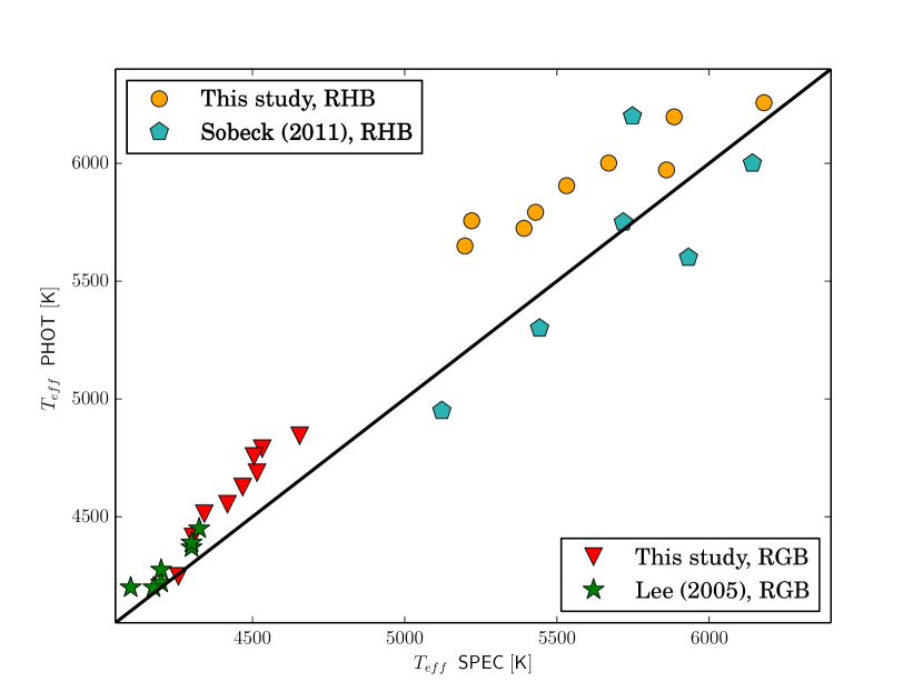
Figure 6: Comparison of photometric and spectroscopic temperatures. Our data agrees well with Lee05, but differs quite significantly from Sob11.

Figure 6 compares the COMB and SPEC $T_{\rm eff}$ values listed in Table 4 for the RGBs and RHBs. $T_{\rm eff}$ values we derived from photometry are systematically higher than spectroscopic ones: $\langle\Delta\mbox{$T_{\rm eff}$}\rangle$ = $\langle\mbox{$T_{\rm eff}$}_{PHOT}-\mbox{$T_{\rm eff}$}_{SPEC}\rangle$ = 159 ($\sigma$ = 80) K for our study. Lee05 found a similar systematic upward shift of photometric temperatures, with their data giving $\langle\Delta\mbox{$T_{\rm eff}$}\rangle$ = 100 ($\sigma$ = 61) K. For the two stars shared by the two studies (117 and 160), differences between their photometric and our COMB $T_{\rm eff}$value are 60 K (star 117) and 32 K (star 160). These small differences are most likely caused by Lee05’s usage of slightly different IRFM calibrations (Alonso et al. 1999), as well as different $(m-M)_{V}$ and $E(B-V)$ values. Overall, the results of the two studies are comparable.

For RHB stars in M68, there exists no previous high-resolution spectroscopic literature reference. We will therefore compare our results to the M15 RHB results of Sob11. The average offset between the photometric and spectroscopic $T_{\rm eff}$ values of our study is $\langle\Delta\mbox{$T_{\rm eff}$}\rangle=321\ (\sigma~{}=~{}146$) K. Sob11 found a much smaller average difference of $\langle\Delta\mbox{$T_{\rm eff}$}\rangle=51\ (\sigma~{}=~{}272$) K. The constant offset between the photometric and spectroscopic $T_{\rm eff}$ values of our study (see Figure 6) suggests that perhaps our adopted reddening value was a bit too high, causing hotter photometric temperatures. Unfortunately, there are no recent M68 RHB studies available that allow us to further explore this difference.

A far greater discrepancy between photometric and spectroscopic parameters is present in derived log(g) values. The RGB side of Figure 5 clearly shows a trend between adopted final $T_{\rm eff}$ and $\Delta$log(g) values (definition given above). In the upper panel of this figure, we have included the Lee05 $\Delta$log(g) values, which exhibit a slight upward trend of $\Delta\mbox{log({\it g})}$ with increasing $(B-V)$ temperature. Our data (middle and bottom panel) shows a similar trend. In the specific case of star 160, Lee05 derive a spectroscopic log(g) of 0.0 dex, whereas we were unable to derive a spectroscopic log(g) value. For the photometric log(g), Lee05 derive a value of 0.7 dex, close to our value of 0.65 dex. Given difference in adopted distance modulus and reddening value, this discrepancy is not serious. For star 117, Lee05 derive a spectroscopic log(g) of 0.3 dex. We were again unable to derive a spectroscopic log(g). The photometric log(g) values are very close, with ours being 0.75 and Lee05 giving a value of 0.8. The average difference between the photometric and spectroscopic log(g) obtained by Lee05 is $\Delta\mbox{log({\it g})}$ = $0.67\ (\sigma=0.10)$, while the difference between our photometric and COMB log(g) values is only $\Delta\mbox{log({\it g})}$ = $0.47\ (\sigma~{}=~{}0.18)$.

The purely photometric study of Carretta et al. (2009, hereafter Car09) also has two RGBs in common with our study, 57 and 79. Since Car09 employed nearly identical $(m-M)_{V}$ and $E(B-V)$ values, differences between our COMB and their final parameters are: -43 K in $T_{\rm eff}$ and -0.31 in log(g) for star 57, while star 79 exhibits differences of -29 K in $T_{\rm eff}$ and -0.44 in log(g). Given the difficulties of analyzing extreme RGB tip stars such as 160 and 117, we lend more weight to the differences between our study and Car09, which, as just demonstrated, are not severe.

The $\Delta$log(g) comparisons for our RHB stars are shown on the right hand side of Figure 5. The top panel shows the Sob11 M15 data, which seems to exhibit a fairly strong $\Delta$log(g)-$T_{\rm eff}$ trend if compared to our data (middle and bottom panel). Our COMB $\Delta$log(g) values give $\langle\Delta\mbox{log({\it g})}\rangle$ = $0.22\ (\sigma~{}=~{}0.09)$, while $\langle\Delta\mbox{log({\it g})}\rangle$ = $0.72\ (\sigma~{}=~{}0.41)$ for our SPEC parameters. The Sob11 data exhibit $\langle\Delta\mbox{log({\it g})}\rangle$ = $0.36\ (\sigma~{}=~{}0.38)$. Clearly, the average differences (dashed lines) as well as $\Delta$log(g)-$T_{\rm eff}$ trends are minimized for our COMB parameters in both the RGB and RHB stars.

As alluded to in §3.1, all of our derived log(g) values would be $\sim$ 0.2 dex lower if we had adopted the Meléndez & Barbuy (2009) based Fe II log($gf$) values, instead of the NIST values. Hence, the $\Delta\mbox{log({\it g})}$ values in Figure 5 would be enhanced by about 0.2 dex. However, even with such an enhanced difference, the current $T_{\rm eff}$ trends would still exist. An additional effect that we have neglected so far is the temperature dependence of the physical log(g) equation given in §4.1. To quantify this effect, we adopted our SPEC temperatures to determine photometric log(g) values, which lowered all of our physical log(g) values by $\sim$ 0.1 dex. Since this value is much lower than our typical log(g) uncertainties (see Table 5), we can safely disregard the $T_{\rm eff}$ dependence of the photometric log(g). In fact, $T_{\rm eff}$ changes of 600 K or more are needed to reproduce log(g) shifts equivalent to our derived log(g) uncertainties. Please see §4.6 for more details.

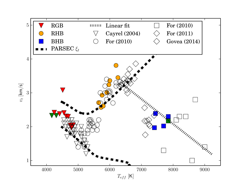
Figure 7: Microturbulent velocities as a function of evolutionary stage. Our results agree well with previous studies and the $\xi_{\rm t}$ calibrations of Gratton et al. (1996). In this Figure, we have used a diamond to represent the RR-Lyrae evolutionary stage. Solid symbols represent this study, while unfilled symbols represent comparison values from previous studies. See §4.3 for more details.

Figure 7 shows a comparison of our derived $\xi_{\rm t}$ to those of previous studies and the calibrations of Gratton et al. (1996). In particular, we used the theoretical PARSEC $T_{\rm eff}$ and log(g) values, applied these to the RGB and RHB $\xi_{\rm t}$ calibrations of Gratton et al. (1996), and plotted the results as thick dashed lines in Figure 7 with the label ‘PARSEC $\xi_{\rm t}$’. Our RGB results agree well with those of previous studies (Cayrel et al. 2004) and the RGB $\xi_{\rm t}$ calibrations in the high temperature end. At low temperatures ($T_{\rm eff}$ $\approx$ 4200 K), our microturbulent velocities seem to deviate from the empirical fits of Gratton et al. (1996). However, since stars in this temperature regime are difficult to analyze, we do not lend much weight to this difference. Individual comparisons with previous studies of Lee05 and Car09 are not possible since Car09, being a purely photometric study, do not give $\xi_{\rm t}$ values and for the two stars shared with Lee05 (116 and 170), we adopted average $\xi_{\rm t}$ values. See §4.2 for more details. Our RHB stars agree well with those of For & Sneden (2010). The PARSEC trend of decreasing $\xi_{\rm t}$ with decreasing $T_{\rm eff}$ is also followed by both our sample and that of For & Sneden (2010). Given this good agreement, we regard our RHB $\xi_{\rm t}$ values as satisfactory. We defer discussion of BHB $\xi_{\rm t}$ values to the next section.

Lastly, we compare the resulting [Fe/H] values of our COMB approach to those of previous studies, which include Car09, Lee05, Behr (2003), and Harris (1996). The difference between our study, which resulted in $\mathrm{[Fe/H]_{M68}}$ = -2.41, and that of Car09 is $\Delta\mathrm{[Fe/H]}$ = 0.15, while for Harris (1996), $\Delta\mathrm{[Fe/H]}$ = 0.18. Lee05 doesn’t give a definite [Fe/H] value, but upon averaging their [Fe I/H] and [Fe II/H] values, we obtain $\Delta\mathrm{[Fe/H]}$ = 0.07. Differences between our study and that of Behr (2003) yield $\Delta\mathrm{[Fe/H]}$ = 0.13. We conclude that there are no significant metallicity differences between our and previous studies.

All of the atmospheric parameters described above were derived without considering Fe NLTE effects. Our assumption of ionization balance, which we used to obtain log(g) values, has been identified as potentially leading to incorrect atmospheric parameters (i.e. Fabrizio et al. 2012 and Bergemann et al. 2012). To quantify the severity of these effects in our sample stars, we used Figure 4 of Bergemann et al. (2012) to estimate NLTE corrections for our derived log(g) values. Unfortunately, we were only able to do this for some of our RGBs (all except 117, 160, 450, 472, and 481). We are currently unaware of any published NLTE calculations for RHB and BHB stars. After applying the NLTE corrections to our RGBs, we found that our log(g) values were raised by approximately 0.3 dex, which, in turn, would essentially eradicate the difference between our PHOT and COMB log(g) values shown in Figure 5. However, it would also lead to greater differences between our atmospheric parameters and PARSEC isochrones. This will be discussed in further detail in §4.5. Since NLTE Fe calculations are only available for a small selection of RGBs in our sample, we decided to ignore these effects for our analysis (see §5 for a discussion of the effects of this choice on derived abundances). A future effort that considers NLTE effects over the whole parameter range of evolved stars in this cluster is welcome.

4.4 Challenges of the BHB stars

The BHB stars in our sample suffer from photometric and spectroscopic deficiencies, which need to be discussed before proceeding to analyze their abundances. Photometric difficulties include the following:

(I) the Ramírez & Meléndez (2005) calibrations for our metallicities become unreliable at approximately 7000K due to a lack of reliable calibration stars

(II) at $T_{\rm eff}$$\ \geq$ 7000K, the peak of the stellar blackbody curve lies at shorter wavelengths than the centers of the B ($\sim$4400 Å) and V ($\sim$5500 Å) bandpasses. Therefore, fluxes are now being measured in the temperature-insensitive Rayleigh-Jeans tail of the Planck distribution, resulting in $T_{\rm eff}$ values that are extremely insensitive to changes in either the B or V flux. Other photometric fluxes (mainly K) are available for some of our stars, but only (B-V) is available for the entire sample. Moreover, the offset between the flux peaks of the BHB stars and V-K bandpasses is worse than for B-V. We therefore did not consider any photometric $T_{\rm eff}$ or log(g) values derived from (V-K).

The spectroscopic temperatures are also afflicted by certain weaknesses. Due to the higher temperatures of the BHB stars, many lines, especially those with high excitation potentials, are not present in their stellar spectra. The reason for this behavior is that the strength of absorption lines is dependent on both the line and continuous absorption. The continuous absorption, mainly due to $H^{-}$ (and neutral $H$ in the violet and near-UV spectral regions), increases sharply with temperature and is much larger in BHB stars than in RHB and RGB stars. In our BHB stars, we therefore see a severe drop-off in the availability of weak high EP lines. The absence of these lines introduces a bias when determining the atmospheric parameters purely from spectroscopic line analysis. Furthermore, the increased temperatures also eliminated one of our atmospheric parameter diagnostic elements, Ti I. The absorption lines of this species are not strong even in RHB stars, and become undetectable in the BHB stars. Given the difficulties in both photometric and spectroscopic approaches, we advise the reader to treat all of the atmospheric parameters of the BHBs with caution. A more involved treatment of M68 BHB stars can be found in Behr (2003).

Our simple analysis of the BHBs, however, seems to produce $\xi_{\rm t}$ values that are somewhat comparable to those of previous studies. Figure 7 shows a comparison of our data to a linear fit (thin dotted line) of the RR-Lyrae of For et al. (2011) and Govea et al. (2014) and the BHB of For & Sneden (2010). For this fit, we have excluded BHB stars with $v\ sin\ i>$ 15 km/s. It has been suggested by Govea et al. (2014) that BHB stars with larger rotational velocities suffer from abnormally large $\xi_{\rm t}$ values; see that study for more details on this point. Our values fit very well with all of the previous data and we therefore regard our microturbulent velocities as satisfactory.

4.5 Comparison of Final Atmospheric Parameters with Isochrones

PARSEC isochrones (Bressan et al. 2012) exhibit several attributes which ultimately led us to choose them as the master isochrones for this project. Most importantly, PARSEC isochrones allow for the computation of isochrones for arbitrary input metallicities and ages. This is due to the usage of two different types of opacities during the calculations. For the low temperature regime, opacities are obtained from the ÆSOPUS code (Marigo 2001), while high temperature opacities are calculated using OPAL 1996 (Iglesias & Rogers 1996) data. Additionally, the latest version of the freely available FREEEOS is used to derive the equations of state. Another very important aspect of the PARSEC isochrones show the $T_{\rm eff}$ - log(g) relationship beyond the tip of the RGB, a usual stopping point for other sets of calculations. All of these improvements over older sets of isochrones should provide a good estimate of the relationship between surface gravities and effective temperatures for different evolutionary states in M68.

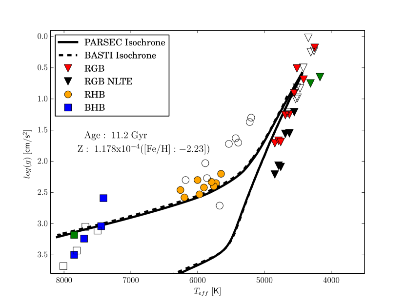
Figure 8: Comparison of isochrone tracks with derived atmospheric parameters. Green markers indicate derivation of atmospheric parameters by photometric data only. Markers without fill indicate purely spectroscopic parameters. See §4.2 for more information.

Figure 8 compares a PARSEC isochrone calculated assuming an age of 11.2 Gyr and a metallicity of Z = 1.178$\times 10^{-4}$ (both consistent with current M68 estimates) with our COMB (filled symbols, usual colors) and SPEC (unfilled symbols) parameters. Overall, our final data matches the PARSEC isochrone much better, providing additional motivation for our COMB approach. We also included NLTE corrected parameters in Figure 8 (black triangles). As mentioned in §4.3, these values show greater discrepancies with the isochrones. To close this now bigger gap between the NLTE parameters and PARSEC isochrones, the metallicity of our evolutionary calculations would have to be increased by $\sim$ 0.4 dex, leading to an inferred $\mathrm{[Fe/H]_{M68}}\sim$ -1.80 dex, a value completely at odds with previous literature studies of this cluster. We also note that isochrone calculations are nearly age independent at M68 metallicities, and thus this difference cannot be accounted for by an adjustment of this input parameter.

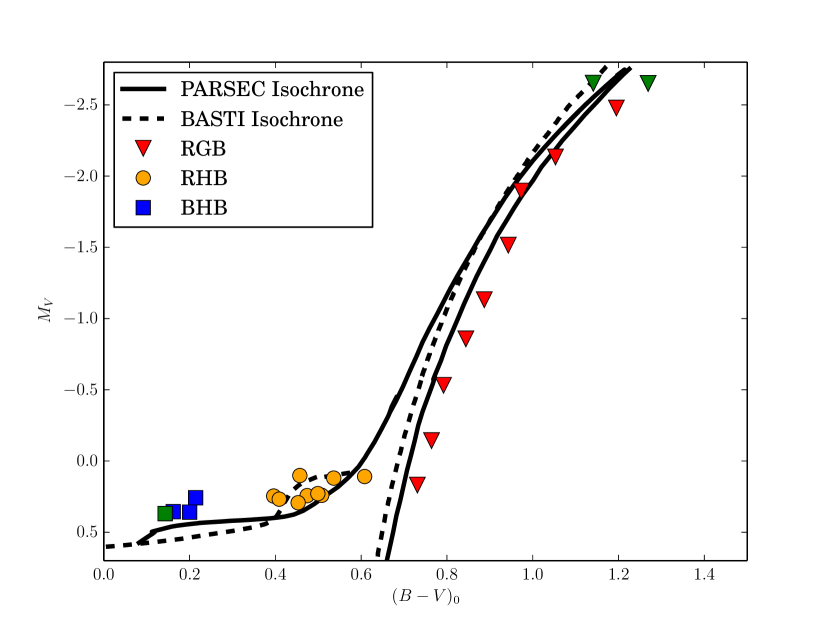
Figure 9: Reproduction of Figure 8, but in color space. The fit of the PARSEC isochrones is somewhat better than that of the BaSTI tracks.

A comparison of the Wal94 photometry data to this isochrone in color space is shown in Figure 9. In both of these figures, we have also included the latest version of BaSTI isochrones (Pietrinferni et al. 2004) with the age and metallicity of M68. In the $T_{\rm eff}$ -  log(g) plane, the difference between the two isochrones is negligible, while in the color plane, the two isochrones give very different answers. The better fit of our data to the PARSEC isochrone tracks in the color plane provides further motivations for using these calculations.

4.6 Uncertainties

Instead of deriving uncertainties for all stars in our sample, we chose representative members of four different evolutionary stages in our sample: lower RGB (172), RGB tip (472), RHB (36) and BHB (337). To obtain the $T_{\rm eff}$ uncertainty, we first calculated the errors in the photometric temperature by considering the color uncertainties given in Wal94. For all of the evolutionary stages, this amounts to $\sigma_{PHOT}\simeq$ 20K for the RGB stars and $\sigma_{PHOT}\simeq$ 70K for RHB stars. Since errors stemming from the scarcity of available measured lines dominate in the BHBs, this part of the error analysis was not performed for this evolutionary stage. In addition to photometric errors, we also considered errors in the reddening, which amounted to $\sigma_{E(B-V)}\simeq$ 10K for the RGBs and $\sigma_{E(B-V)}\simeq$ 45K for RHBs. The measurement uncertainty contribution to our total $\sigma_{\mathrm{\mbox{$T_{\rm eff}$}}}$ was simulated by adjusting the temperature of stars until we achieved a shift in Fe I abundances equal to the standard deviation of the abundances implied by the stellar Fe I lines. The errors from the photometry and measurements were added in quadrature to give the final $T_{\rm eff}$ uncertainty. Uncertainty in log(g) was then determined by applying the upper and lower values of $T_{\rm eff}$ to our stars and then again requiring ionization balance. For $\xi_{\rm t}$ uncertainties, we repeated the process that we used to determine final atmospheric parameters (see Sec. 4.2), but this time applying the upper and lower temperature limits. The final uncertainties determined in this manner can be found in Table 5. We did not consider atmospheric metallicities in our error analysis, as they have a negligible effect on total parameter errors.

The differences in uncertainties between the evolutionary stages is easily explained. Atmospheres of RGB stars are much more sensitive to $T_{\rm eff}$ and log(g) changes than the more evolved stars due to the greater number of observed lines and greater range of excitation potentials, ionization state and log(gf) values. As $T_{\rm eff}$ and log(g) increase, we see a drop off in the number of observed lines and therefore less sensitivity to changes in atmospheric parameters. Hence, our RHB have larger uncertainties than our RGBs, but smaller uncertainties than the BHBs, just as expected.

5 ABUNDANCE ANALYSIS

In this section we present the results of our abundance analysis. Unlike the discussion of the atmospheric parameters, we will discuss these not individually by evolutionary stage, but rather attempt to give an overview of post main sequence stars in M68. All of the following abundances are derived using the COMB parameters given in Table 4. Table 8 gives average abundances in standard [X/Fe] fashion for each star in our sample, while Table 9 summarizes the average abundances for each evolutionary stage and M68 as a whole. The first two lines in these tables give [Fe/H] for the corresponding star/evolutionary stage. We note here that the Fe I and Fe II of stars 117 and 160 do not agree. The reason for this non-agreement is explained in §4.2.

For completeness, we will now briefly discuss the sensitivites of our abundances to the adopted atmospheric parameters, which we determined by deriving abundances using the SPEC and PHOT parameters given in Table 4 for stars 472, 172, 36, and 337 (stars used to derive atmospheric parameter uncertainties). Since we did not derive PHOT $\xi_{\rm t}$ and [Fe/H] values, we adopted those of the COMB approach for the stars listed above. This is justified by repeating the analysis described in §4.2, but this time fixing log(g) to the photometric value, which showed that the resulting PHOT $\xi_{\rm t}$ and [Fe/H] values differ very little from those of the COMB approach. The derived absolute abundances shifted as a result of the adoption of the PHOT and SPEC parameters, but the metallicity, which we use to normalize our abundances, changed by approximately the same amount (see Table 4). Therefore, the resulting normalized abundances differed from the COMB abundances by less than the abundance uncertainties discussed in §5.3 and listed in Table 5. We thus anticipate no serious changes to our derived abundances due to the adoption of either the PHOT or SPEC parameters.

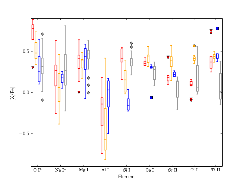
Figure 10: Comparisons of derived abundances for 8 $\leq Z\leq 22$. Any abundance differences between the evolutionary stages are explained in §5.1. Solid markers outside the boxes represent outlier abundances. Grey boxes represent data from previous studies. Elements marked with ‘*’ have NLTE corrections applied to them.

A summary of the element ratios ([X/Fe]) for $8\leq Z\leq 70$ in box-plot form can be found in Figures 10, 11, and 17. Unfortunately, the quality of our spectra did not allow us to make any inferences about differences in He abundances between M15 and M68 (see §1 for more details). As before, red data represents the RGB, yellow data represents the RHB, and the blue data shows the BHBs. We have also added data from previous studies, which is shown as grey boxes. In these box plots, the mean elemental abundance is represented by the central bar, while the upper and lower edges of each box give the first (lower edge) and third (upper edge) quartile of the plotted data. The whiskers constitute a $\sim 3\sigma$ boundary. Outlier data beyond the whiskers is depicted as solid symbols with corresponding colors. Table 7 gives a summary of previous studies used for comparison in Figures 10, 11, and  17. A list of lines, as well as the method used to derive the abundances (EW or synthesis) are given in Table 3.

5.1 Light and Fe-Group Elements

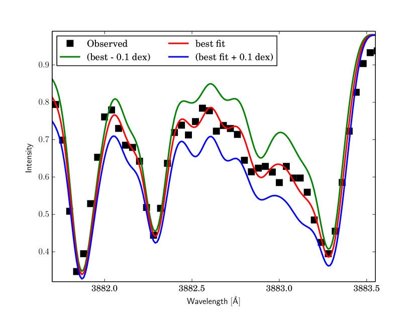
Figure 12: Synthesis of the CN region around 3880 Å. Noise limitations are evident from this plot. The spectrum shown here is a co-addition of stars 117, 160, 472, and 481, all of which are RGB tip members.

Carbon and Nitrogen: Due to the low metallicity of M68 and the S/N limitations of our spectra, determining C I and N I abundances for our sample stars was very difficult. After co-adding the spectra of our four coolest RGB stars, we were able to estimate $\langle$¹²C/¹³C$\rangle$ $\simeq$ 5$-$7 for the coolest giants in M68. The quality of our stellar spectra precluded determination of values for individual stars. Better quality data are needed to make a more accurate carbon isotopic assessments. However, these results are in line with the low ¹²C/¹³C values obtained for other globular clusters such as M3 (¹²C/¹³C $\approx$ 6, Pilachowski et al. 2003), M4 (¹²C/¹³C $\approx$ 5, Brown & Wallerstein 1989), and M22 (¹²C/¹³C $\approx$ 6, Smith & Suntzeff 1989). Assuming a ¹²C/¹³C value of 6, we then were able to estimate [C/Fe] $\sim$ -0.5, and [N/Fe] $\sim$ 1. Figure 12 shows the co-added RGB tip spectra and a corresponding synthesis for the CN region around 3880 Å. Noise limitations are evident, even in these co-added spectra. C I and N I abundances will not be further considered in this paper given the difficulties in trying to determine these abundances.

Oxygen and Sodium: The O I abundances for the RGB stars in our sample were determined by synthesis of the [O I] 6300.3 Å line, while for three of our RHB and all of the BHB stars, oxygen abundances were determined from the O I triplet at 7771.94 Å, 7774.17 Å, and 7775.39 Å. NLTE corrections are negligible for any forbidden transitions, but such effects can be quite large for abundances derived from the O I triplet (eg., Sitnova et al. 2013 and references therein). We used the estimates given in their Table 11 to extrapolate NLTE corrections for our final temperatures by deriving a logarithmic relation between these corrections and temperature, which is given by:

$$\mathrm{[O/Fe]_{NLTE}-[O/Fe]_{LTE}}=-1.43\ \mathrm{log_{e}}(\mbox{$T_{\rm eff}$})+12.066.$$

NLTE corrections for our stars range from $-$0.35 dex to $-$0.76 dex.

Na I abundances in our stars were derived using EW measurements from four Na I lines: 5889.95 Å, 5895.92 Å (the D lines), 8183.26 Å, and 8194.82 Å. The EWs for these lines can be found in Table 3. We derived NLTE corrections using the INSPECT web interface, which is based on Lind et al. (2011). Unfortunately, the parameters of some of our stars exceed the $T_{\rm eff}$- log(g) limits. For such parameters, we extrapolated the NLTE corrections given by the websites to our specific log(g) and $T_{\rm eff}$ combinations. In the case of RGB stars, the limit was set by log(g) as the website did not accept values lower than 1.00. For the BHB stars, the limit was set by $T_{\rm eff}$. NLTE corrections obtained is this manner should not be viewed as definite, but rather as zeroth order estimates.

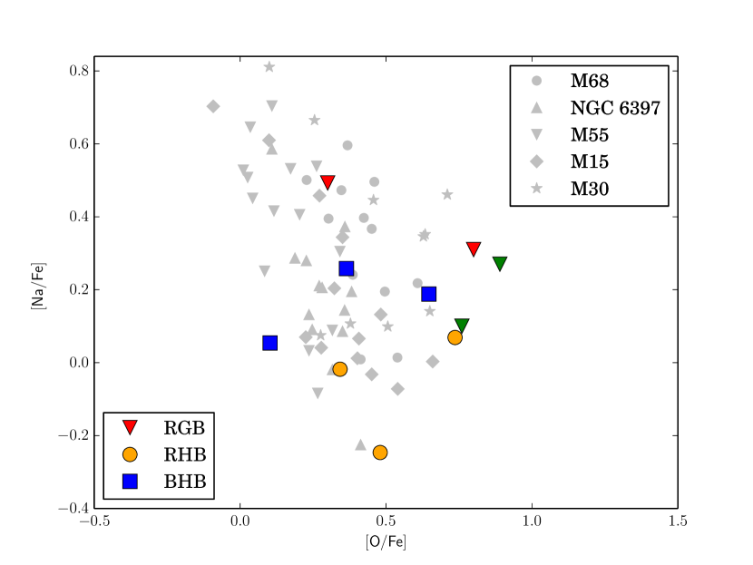
Figure 13: Correlation between [Na/Fe] and [O/Fe]. Our data is compared to that of Car09, who derived these abundances for RGBs in M68, NGC 6397, M55, M15, and M30. NLTE corrections have been applied to for both O and Na abundances.

From Figure 10, it seems that O I abundances are enhanced in our RGB stars as compared to other evolutionary stages and previous studies. However, since we are using different features to determine the O I abundances in different evolutionary groups, caution is warranted when interpreting this abundance trend. In Figure 13, we compare Na I and O I abundances. The anti-correlation of these two elements, which seems to be exclusive to GCs, has been confirmed by many studies (Car09, Gratton et al. 2004 and references therein). It is currently believed that this trend results from pollution of the cluster medium by an earlier generation of stars (Gratton et al. 2004). Unfortunately, we cannot confidently say that we observe such an anti-correlation in our sample, since we were only able to derive both Na I and O I abundances for 11 out of our 25 stars. However, the abundances derived for these stars fall within the same general ranges, perhaps slightly elevated, as those of Car09 (grey symbols), which consist of some of the most metal-poor GCs known: NGC 6397 ([Fe/H] $\approx$ -2.02), M55 ([Fe/H] $\approx$ -1.94), M15 ([Fe/H] $\approx$ -2.37), and M30 ([Fe/H] $\approx$ -2.27). All quoted metallicities were obtained from Harris (1996). Data for stars 117 and 160 (see §4.2 for more details) are shown in green again. These two stars seem to have particularly high [O/Fe] values, which, in light of the problems associated with deriving their atmospheric parameters, are no cause for serious concern. We conclude that, on average, M68 is not overabundant in sodium, but our data does suggest an oxygen overabundance. Additionally, if our data is combined with the Car09, we clearly see an anti-correlation of our derived oxygen and sodium abundances. A closer look at Figure 13 also appears to reveal a systematic difference of O I abundances between the RGB, RHB, and BHB. Such differences have been observed and analyzed by several other authors (see Marino et al. 2011 and references therein). Given that we employed different lines to obtain our abundances of each of the evolutionary stages and relied on crude corrections to account for NLTE effects, we will not attempt to dissect the details of these differences here.

We now compare our oxygen abundance results with those of Lee05 and Car09. Car09 derived similar oxygen abundances also using the 6300.3 Å [O I] transition for several different GCs. The average metallicity for the Car09 M68 stars is slightly higher than ours, and since they adopted purely photometric log(g) and $T_{\rm eff}$ values, their slightly lower O I abundances are expected. In the specific case of the two overlapping RGBs, the differences are $\Delta$[O/Fe]₅₇ = $-$0.35 for star 57, while for star 79 we could not derive an O I abundance. The discrepancy between our results and those of Lee05 are more difficult to understand. For star 160, $\Delta$[O/Fe]₁₆₀ = $-$0.43 and for star 117 $\Delta$[O/Fe₁₁₇] = $-$0.53. However, Lee05 employed a very different atmospheric parameter derivation methodology. Furthermore, they did not force ionization balance between neutral and ionized Fe lines, resulting in Fe II abundances that are on average, 0.37 dex higher than the corresponding Fe I abundances. They chose to normalize their oxygen abundances using these elevated Fe II values, naturally leading to higher [O/Fe] ratios.

The differences between our sodium abundances and those of Car09 are $\Delta$[Na/Fe]₅₇ = $+$0.17, and $\Delta$[Na/Fe]₇₉ = $+$0.14 . These differences can mostly be attributed to the slightly different parameter derivation methodology and NLTE correction algorithm employed by Car09. The discrepancies between our work and that of Lee05 are a bit greater: $\Delta$[Na/Fe]₁₁₇ = $-$0.27 and $\Delta$[Na/Fe]₁₆₀ = $+$0.36. Again, these differences, considering the disparate approaches, are negligible. We note here that Na I NLTE corrections could not be derived for star 160 using the methods described above.

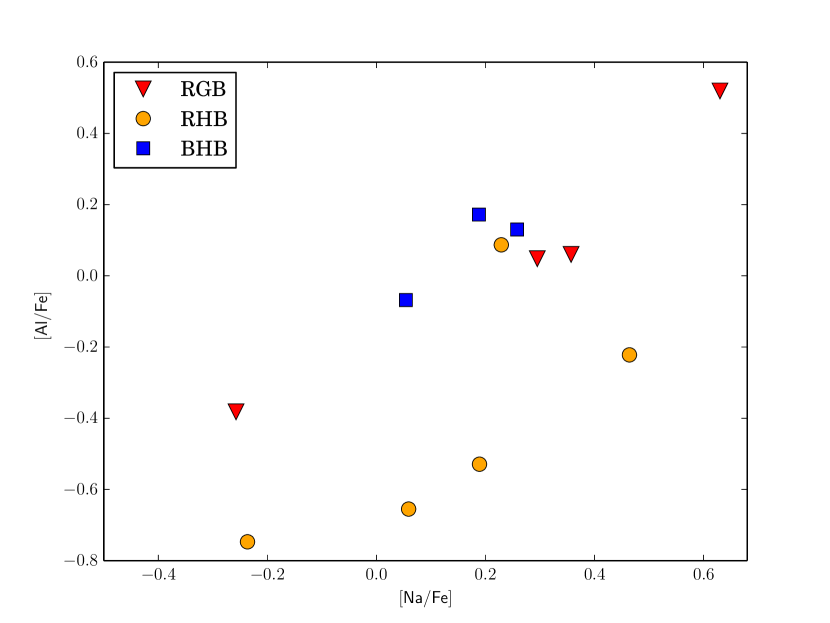
Figure 14: The classical comparison of [Na/Fe] to [Al/Fe], which produces the standard result for globular cluster studies. In this plot, NLTE corrections were applied only to Na.

Aluminum: All of our aluminum abundances were derived from the Al I resonance lines at 3944.01 Å and 3961.53 Å. Due to severe NLTE effects, these lines are known to give abundances which are, on average, a factor of 6 lower than those derived from other Al I lines (e.g., Baumüller & Gehren 1997, Andrievsky et al. 2008). Unfortunately, these are the only measurable Al I lines in our spectra. In their Figure 2, Andrievsky et al. 2008 give NLTE corrections applicable to some of our giants. We estimate corrections of 0.4 dex for stars 79 and 172, a correction of 0.55 dex for stars 226 and 256, and a correction of 0.5 for star 440. Atmospheric parameters for all other stars in our sample are outside the recommended limits of Andrievsky et al. (2008) and therefore are not considered for NLTE corrections. Table 6 gives the NLTE Al I abundances, as well as NLTE corrected Na I abundances. Clearly, there is a spread amongst Al I abundances in M68. However, all low/high [Al/Fe] ratios correspond to low/high [Na/Fe] ratios. Figure 14 shows this well-known correlation between [Al/Fe] and [Na/Fe] for globular clusters (e.g Car09, Ivans et al. 2001, and Shetrone 1996). In the interest of having the maximum number of data points available, we decided to use the Al I LTE abundances. Since the NLTE corrections are almost constant for our stars (see discussion above and Table 6), there is no danger in destroying any abundance correlations by using the LTE abundances. The clearly positive correlation between these two elements provides evidence for primordial abundance enhancements by earlier generations of stars. We will not attempt to explore these primordial abundance enhancements using our data, but refer the reader to Gratton et al. (2004) for more information.

Lee05, who derive $\langle\mathrm{[Al/Fe]}\rangle$ = 1.08, and Car09, who derive $\langle\mathrm{[Al/Fe]}\rangle<$ 0.74, measured their abundances using the subordinate Al I lines at 6696.03 Å and 6698.67 Å. We note that Car09 explicitly state that all their Al I abundances are upper limits, which, in combination with the statement by Andrievsky et al. (2008) that these subordinate lines should not be visible at [Fe/H] $\lesssim$ $-$2.5, leads us to lend less significance to the differences between our study and Lee05. We derive $\langle\mathrm{[Al/Fe]_{NLTE}}\rangle$ = 0.31, which given the difficulties explained above, seems in concord with Car09. To ensure that our lack of detection of these subordinate lines is not caused by noise limitations, we co-added RGB spectra of the stars with the highest Al I abundances implied by the resonance lines. Despite these efforts, we were not able to measure the subordinate lines, or Al I line at 7836.14 Å, which suggests that [Al/Fe] $<$ 0.78.

$\alpha$ Elements: The $\alpha$ and $\alpha$-like elements considered in this study are Mg I, Si I, Ca I, and Ti I/Ti II. Their abundances, which were obtained from $EW$ measurements, are compared in Figure 10. We will discuss them in order of increasing $Z$.

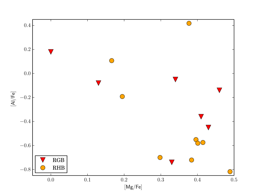
Figure 15: Anti-correlation of [Al/Fe] and [Mg/Fe] for stars in our sample.

Mg I abundances for all evolutionary stages show good agreement, which, in combination with Figure 15, where we see the expected [Mg/Fe]$-$[Al/Fe] anti-correlation, supplies further evidence for primordial abundance variations in GC stars. Dissecting the details of these abundance behaviors is beyond the scope of this paper. Here, we mainly demonstrate that our atmospheric parameter derivation approach reproduces all the classical abundance hallmarks of any GC study. Star 202, with [Al I/Fe] $\sim$ 0.4 in Figure 15 is the hottest RHB in our sample, and with $T_{\rm eff}$ = 6257, very close to the RR-Lyrae gap. Therefore, the Al I abundances for this star could be compromised. We have also chosen not to include BHB Mg abundances in Figure 15 due to reasons listed in §4.4.

Car09, Lee05 and Behr (2003) also derived Mg I abundances for their stars. They differ from our measurements as follows: $\Delta_{Mg/Fe,57}$ = -0.044, $\Delta_{Mg/Fe,79}$ = -0.083, $\Delta_{Mg/Fe,117}$ = -0.25, and $\Delta_{Mg/Fe,160}$ = -0.01. All of these ratios show excellent agreement, except those of star 117. The large discrepancy for this star, however, is no real surprise given the hugely different approaches for determining atmospheric parameters and the fact that this particular star might be an example of an extreme RGB tip star, making its analysis very difficult. We will not compare the individual stellar abundances for star 324 with those of Behr (2003), since we were unable to derive proper atmospheric abundances for this particular star. Behr (2003) derive a $\langle$[Mg/Fe]$\rangle$ = 0.18, while we obtain $\langle$[Mg/Fe]$\rangle$ = 0.35 for our BHBs. This difference can be explained by the different approach taken by Behr (2003) to derive their atmospheric parameters.

Unlike the [Mg/Fe] ratios, our derived [Si/Fe] abundances show large discrepancies between the evolutionary stages. This is because, as several studies have shown, Si I abundances drop with increasing $T_{\rm eff}$ (e.g. Figure 10 of Preston et al. 2006 and references therein). In the interest of consistency, we derived all of our Si I abundances from the 3905.53 Å line, which is saturated in the RGB, leading to possibly unreliable abundances. If we had used the 4102.94 Å Si I line for this evolutionary stage, our RGB abundances would be elevated by about 0.4 dex. Unfortunately, the 4102.94 Å line is not measurable in the RHBs or BHBs.

For the RGB branch, our study yields $\langle$[Si I/Fe]${}_{\mathrm{RGB}}\rangle$ = 0.40 (see Table 9), which, if compared to $\langle$[Si I/Fe]${}_{\mathrm{RGB}}\rangle$ values from other metal poor clusters: $\langle$[Si I/Fe]${}_{\mathrm{RGB,M15}}\rangle$ = 0.55, and $\langle$[Si I/Fe]${}_{\mathrm{RGB,M92}}\rangle$ = 0.59 (both from Sneden et al. 2000), seems slightly too low. However, Sneden et al. 2000 use only the 5948.55 Å Si I line, and a different set of $gf$ values. Similar to Sneden et al. (2000), Lee05 also derive an analogously high Si I abundance, $\langle$[Si I/Fe]${}_{\mathrm{RGB,M68}}\rangle$= 0.71, which they base on EW measurements of 6-7 mÅ for all their stars. Given that their S/N is comparable to ours, noise limitations could contribute to their derived Si overabundances. To ensure that our EW measurements are not at fault, we calculated the EW values needed to reproduce the Lee05 abundance for several different high excitation Si I lines, including those used by Lee05. Subsequently, we inspected the spectra of our stars for these lines and tried to measure the EW needed to reproduce the Lee05 abundances. We were unable to measure or visually locate any of these lines in our spectra, confirming that M68 most likely does not exhibit an Si overabundance. In their study, Car09 derive $\langle$[Si/Fe]$\rangle$ = 0.40, in good agreement with our derived value.

Our RHB Si measurements yield $\langle$[Si/Fe]$\rangle$ = 0.16, which is in accord with Preston et al. (2006), who derive $\langle$[Si I/Fe]${}_{\mathrm{RHB,M15}}\rangle$ = 0.32. While we expect lower abundances with increasing $T_{\rm eff}$ (see above), a drop of 0.5 dex in [Si/Fe] between our average RHB abundances and those of Lee05 would be outside of the usual range found by previous studies.

As a final remark on Si I abundances, we perform a star-by-star comparison with Car09, which yields these differences: $\Delta_{Si/Fe,57}$ = $-$0.23, $\Delta_{Si/Fe,79}$ = $-$0.051, The reasons for the large differences are explained above and can also be attributed to the different methodologies employed for deriving these abundances and associated atmospheric parameters. We were unable to derive Si abundances for either stars 117 or 160, precluding us from a comparison with Lee05.

Perhaps a more important and reliable diagnostic than Si is Ca, which exhibits more measurable transitions and has been shown to give constant abundances for GCs with [Fe/H] $<$ -1.00. Our analysis yields $\langle$[Ca/Fe]${}_{\mathrm{M68}}\rangle$ = 0.36, very much in line with previous studies shown in Figure 4 of Gratton et al. (2004). They derive $\langle$[Ca/Fe]$\rangle$ =+0.25 ($\sigma$ = 0.02) for 28 clusters with [Fe/H] $<$ -1.00. A comparison with Lee05, who also derive Ca I abundances yields the following: $\Delta_{Ca/Fe,117}$ = -0.16, and $\Delta_{Ca/Fe,160}$ = -0.04. For a thorough review on Ca abundances in GCs, please see Gratton et al. (2004).

As a final $\alpha$ element, we measured the abundances of Ti I and Ti II, whose abundances provide a good diagnostic of possible over-ionization in stellar atmospheres. We will not compare our Ti abundances to those of Lee05, since the methodology of the two studies are too disparate. A quick look at Figure 10 reveals over-ionization in RGB stars (Ti II abundances are, on average, 0.34 dex higher), while the agreement between Ti I and Ti II is excellent for RHB stars. For reasons explained above, there are no measurable Ti I lines in our BHB stars. Overall, our data shows an $\alpha$ element enhancement, as expected from globular clusters. A similar enhancement in M68 was found by Behr (2003).

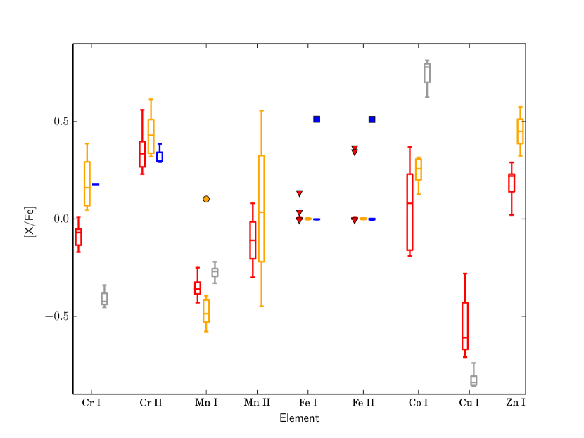
Figure 11: Continuation of Figure 10, but with 24 $\leq\ Z\ \leq 30$. Abundance differences are discussed in §5.1.

Fe-peak Elements: Sc II, Cr I, Cr II, Mn I, Mn II, and Co I make up the $Fe$-peak elements measured in this study. Their combined mean abundances are $\langle$[X/Fe]${}_{Fe\ \mathrm{peak}}\rangle$ = 0.11 ($\sigma$ = 0.30). Figures 10 and 11 show the behavior for these elements amongst different evolutionary stages. Sc II abundances agree for all our evolutionary states and the Lee05 data. The large difference between Cr I and Cr II abundances could be a cause for concern, since we required ionization equilibrium for our abundances. However, such behavior has been observed in other cluster as well as field stars and is currently unexplained (see Preston et al. 2006 and references therein). In Figure 11, we show a comparison with the M92 data of Langer et al. (1998). Clearly, their average abundance is much lower than ours. Due to the known problems with this element, however, we will not lend too much weight to this difference.

Mn I and Mn II abundances also seem to show over-ionization and large variations amongst individual stars. However, nearly all of these abundances are based on a single stellar line measurement. We therefore urge the reader to treat these abundances with caution. Co I abundances show agreement between the RGB and RHB branches, but are again much lower than those of Langer et al. (1998). The reasons for this behavior are unknown.

Lee05 measured Mn I and Sc II, and for these species our differences are: $\Delta_{Sc/Fe,117}$ = -0.24, $\Delta_{Sc/Fe,160}$ = -0.26, $\Delta_{Mn/Fe,117}$ = 0.03, and $\Delta_{Mn/Fe,160}$ = -0.04. Unfortunately, no other abundance comparisons are possible.

Copper and Zinc: The last two elements in Figure 11 are Cu I and Zn I. Lee05 also derived Cu I abundances and the difference between the overlapping star 160 is $\Delta_{Cu/Fe,160}$ = -0.55. These differences can be attributed to the disparate approaches in deriving atmospheric parameters. For Zn I, no previous references exist.

5.2 Heavy Elements

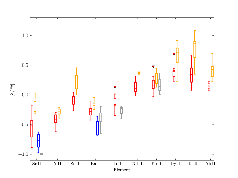
Figure 17: Abundances of n-capture elements amongst the different evolutionary stages. A slight r-process enrichment can be observed. Further details are given in §5.2

n-capture Elements: Figure 17 shows box plots of the distribution of n-capture elements in our stars. Unlike many previous studies, the violet extent of our spectral coverage allows us to include rare-earth-element species such as Dy II and Yb II. The distribution of n-capture elements can be used to infer $r$- or $s$-process enrichment (see Figures 1, 2, and 10 in Sneden et al. 2008). As part of $r$-process enrichment, we should observe low [Ba/Eu] and [La/Eu] ratios, both of which are clearly present in our sample. We therefore conclude that M68, much like other metal poor GCs (e.g. Sobeck et al. 2011), exhibits $r$-process enrichment. The constant offset of $\sim$ 0.26 dex between the RGB and RHB evolutionary stages can be attributed to the usage of different MOOG versions (see §4.2 for more details), as well as general difficulties associated with the size of the parameter space covered by this study.

Figure 17 also demonstrates discrepancies between Sr II and Ba II abundances amongst the evolutionary stages. These are easily explained. For Sr II, the employed lines at 4077.71 Å and 4215.52 Å are saturated in almost all RGB and RHB stars, resulting in unreliable abundances. In the hottest RHB and all BHB stars, these Sr II lines are unsaturated and yield consistent abundances. The Ba II discrepancies can be traced back to the usage of different sets of lines for obtaining abundances. The well known 4554.03 Å Ba II line is saturated in our RGB and RHB stars, and we used the 5853.69 Å, 6141.73 Å, 6496.91 Å in these stars. In our BHB stars, these Ba II lines were not available, so we reverted to the 4554.03 Å line.

Car09 did not derive any n-capture process abundances, and therefore we will compare all of our abundances to those of Lee05. The differences for star 117 are $\Delta_{Ba\ II/Fe,117}$ = -0.28 (only element available for comparison), while those for star 160 are $\Delta_{Ba\ II/Fe,160}$ = -0.29, $\Delta_{La\ II/Fe,160}$ = -0.25, and $\Delta_{Eu\ II/Fe,160}$ = -0.14. Like before, $\Delta_{X/Fe}$ is defined to be [X/Fe]${}_{previous\ study}$ $-$ [X/Fe]${}_{this\ study}$. Possible reasons for the differences between our abundances and those derived by Lee05 have been discussed in §5.1.

5.3 Abundance Uncertainties

Much like atmospheric parameter uncertainties, we derived representative abundance $\sigma$ values for each evolutionary state in our sample. The representative stars remain the same: 472 (RGB tip), 172 (lower RGB), 36 (RHB), and 337 (BHB). We note that we derived Cr I abundance uncertainties for the BHBs using star 289, since we could not measure any Cr I lines in star 337.

To obtain uncertainties for elements whose abundances are based on EW measurements, we took the following approach: Uncertainties for any element for which more than 3 lines were measured, the standard deviation of the abundances implied by the measured lines was used. For any element with less than 3 lines, we re-measured the EW now considering factors such as continuum placement and smoothing. Using these re-measured EW values, we derived new abundances, which allowed us to calculate uncertainties for the corresponding species. This method led to uncertainties of $\simeq$ 0.13 dex for most elements.

For uncertainties for elements where spectral synthesis was used to obtain abundances, we re-synthesized the spectra and again considered factors such as continuum placement, smoothing and assumed abundance. Just like with our EW uncertainties, this method leads to final $\sigma$ values of $\simeq$ 0.13 dex. The final uncertainties obtained in the above described fashions can be found in Table 10. It is also mentioned here that our uncertainties in $T_{\rm eff}$, log(g), and $\xi_{\rm t}$ lead to additional uncertainties of 0.2 - 0.3 dex, which are not included in the results of Table 10.

6 CONCLUSIONS

In this paper, we have explored the atmospheric parameters and detailed chemical compositions of 25 evolved members of M68. Particular attention has been paid to comparisons of the assets and liabilities of photometrically based and spectroscopically based parameters. From the discussion in §4.2, and the evidence presented in §4.3, it is now clear that difficulties in deriving atmospheric parameters in an internally consistent manner over a parameter space that covers $\sim$ 4000 K in $T_{\rm eff}$, and $\sim$ 3.00 dex in log(g) exist and need to be accounted for. Luckily, for M68, as for almost any cluster, we have reliable reddening and distance moduli that allowed us to treat these problems by creating a hybrid spectroscopy-photometry approach.

Some of the discovered weaknesses of the two standard approaches include photometric derivation of log(g) values. As mentioned in Sec. 4.1, the physical log(g) depends on the mass of the star in consideration. Unfortunately, precise mass loss between the turn-off, RGB and later evolutionary stages is still uncertain. Our method of applying a single mass to all stars in our sample provides a good zeroth order approximation of the physical log(g), but for increasingly detailed studies, more accurate stellar masses should be adopted. Spectroscopic weaknesses include scarcity of lines in hotter RHB and BHB stars, as well as serious metallicity trends (see Figure 4). A combination of both the photometric and spectroscopic methods allowed us to address most of these problems. One of the main highlights of our final adopted approach is the lack of any obvious metallicity difference between evolutionary stages (see Figure 4 or $\langle$[Fe/H]$\rangle$ values for RGBs and RHBs in Table 9). Our analysis results in $\sigma_{\mathrm{\langle[Fe/H]\rangle}}$ = 0.14, for all stars, including the BHBs. We remind the reader that this lack of metallicity difference is not inherent to our analysis or our atmospheric parameter derivation method. Instead, it naturally grows out of our adoption of photometric temperatures, making this result even more remarkable.

In addition to the metallicities being in good agreement, Table 9 shows that the abundances for all other elements agree across the different evolutionary stages. For the elements that seem to exhibit any discrepancies, a valid and detailed explanation is given in §5. We can therefore conclude that even though we adopted a non-standard, hybrid approach to deriving our atmospheric parameters, the resulting abundances are what one would expect from a classical purely spectroscopic analysis. Moreover, we were also able to reproduce all classical hallmarks of GC populations, such as the [Na/Fe]$-$[O/Fe] and [Mg/Fe]$-$[Al/Fe] anti-correlations, Ca and Si abundances that agree with previous studies, as well as slight $r$-process enrichment. In the absence of very detailed NLTE calculations and/or 3D model atmospheres, such a hybrid approach may be necessary for us to further develop our understanding of cluster stars, at least from a stellar atmospheric perspective.

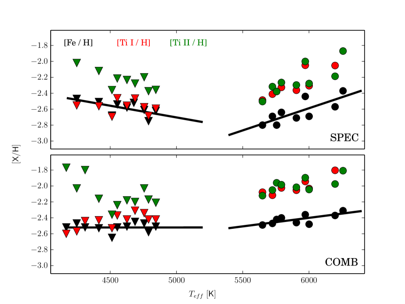
Figure 4: Comparison of ionization and metallicity effects using different atmospheric parameters. The solid black line represents a linear fit to [Fe/H] of RGB and RHB stars as a function of temperature.

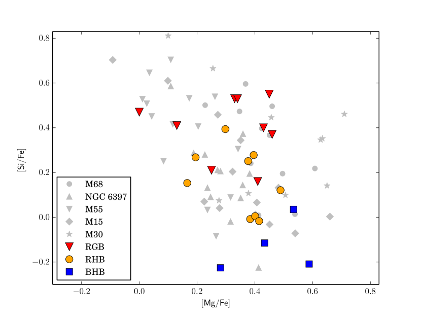
Figure 16: Correlation between Si and Mg abundances. The drop-off in the Si abundances with increasing temperatures is well known.

Table 1: Fundamental parameters of NGC 4590

Right ascension1	12 36 27.98
Declination1	-22 44 38.6
Distance4	10.3 kpc
Age3	11.2 Gyr
Metallicity4	-2.23
$E(B-V)$4	0.05
$(m-M)_{V}$4	15.210

Table 2: Photometric parameters

Star	V	(B-V)	(V-I)
RGB photometry
57	14.213	0.937	1.116
79	13.830	0.993	1.161
117	12.693	1.191	1.320
160	12.694	1.319	1.418
172	14.488	0.894	1.084
226	15.514	0.781	0.981
256	15.202	0.814	1.004
440	14.814	0.842	1.030
450	13.450	1.023	1.182
472	13.211	1.103	1.244
481	12.867	1.245	1.359
RHB photometry
36	15.588	0.524	0.723
47	15.545	0.567	0.775
202	15.591	0.446	0.676
334	15.586	0.558	0.727
403	15.465	0.586	0.798
454	15.447	0.507	0.740
458	15.638	0.503	0.700
533	15.574	0.549	0.746
547	15.613	0.459	0.685
BHB photometry
170	15.714	0.193	0.323
289	15.603	0.264	0.295
324	15.772	0.204	0.287
377	15.701	0.212	0.348
391	15.704	0.250	0.311

Table 3: EW lists

				57		79		117
Ion	$\lambda$ (Å)	E.P. (eV)	log(gf)	EW	log $\epsilon$	EW	log $\epsilon$	EW	log $\epsilon$	Method	Ref.
O I	6300.30	0.000	-9.820	$\cdots$	7.07	$\cdots$	7.04	$\cdots$	7.15	synth	1
	7771.94	9.150	0.370	$\cdots$	$\cdots$	$\cdots$	$\cdots$	$\cdots$	$\cdots$	EW	2
	7774.17	9.150	0.220	$\cdots$	$\cdots$	$\cdots$	$\cdots$	$\cdots$	$\cdots$	EW	2
	7775.39	9.150	0.000	$\cdots$	$\cdots$	$\cdots$	$\cdots$	$\cdots$	$\cdots$	EW	2
Na I	5889.95	0.000	-0.190	$\cdots$	$\cdots$	221.6	3.97	$\cdots$	$\cdots$	EW	3
	5895.92	0.000	0.110	205.5	4.19	194.2	3.94	$\cdots$	$\cdots$	EW	3
	8183.26	2.100	0.240	67.1	4.21	55.5	4.01	75.1	4.06	EW	3
	8194.82	2.100	0.490	111.9	4.53	82.5	4.10	112.6	4.27	EW	3
Mg I	3829.36	2.710	-0.227	$\cdots$	$\cdots$	232.6	5.47	$\cdots$	$\cdots$	EW	4
	3832.31	2.710	0.125	$\cdots$	$\cdots$	$\cdots$	$\cdots$	$\cdots$	$\cdots$	EW	4
	4571.10	0.000	-5.623	105.9	5.54	106.3	5.41	158.9	5.59	EW	4
	5172.70	2.710	-0.393	$\cdots$	$\cdots$	$\cdots$	$\cdots$	135.6	5.86	EW	4
	5183.62	2.720	-0.167	$\cdots$	$\cdots$	$\cdots$	$\cdots$	$\cdots$	$\cdots$	EW	4
	5528.42	4.350	-0.498	100.3	5.54	117.1	5.74	$\cdots$	$\cdots$	EW	4
Al I	3944.01	0.010	-0.638	$\cdots$	$\cdots$	215.2	4.16	$\cdots$	$\cdots$	EW	3
	3961.53	0.010	-0.336	$\cdots$	$\cdots$	177.2	3.43	$\cdots$	$\cdots$	EW	3
Si I	3905.53	1.910	-1.041	293.6	5.55	255.2	5.36	$\cdots$	$\cdots$	EW	5
Ca I	4226.74	0.000	0.244	$\cdots$	$\cdots$	$\cdots$	$\cdots$	$\cdots$	$\cdots$	EW	6
	5588.76	2.530	0.210	69.1	4.12	73.7	4.13	95.1	4.26	EW	6
	5857.46	2.930	0.230	51.1	4.30	43.0	4.14	66.6	4.31	EW	6

Note. — The machine-readable version of the entire table is available in the online journal. A portion of the table is shown here for guidance concerning form and content. The abundances listed in this table are given for corresponding individual transitions.

Table 4: Atmospheric parameters

		PHOT		SPEC		COMB
Star	S/N	$T_{\rm eff}$	log(g)	$T_{\rm eff}$	log(g)	$T_{\rm eff}$	log(g)	[Fe/H]	$\xi_{\rm t}$
RGB parameters
57	140	4626	1.54	4468	0.83	4626	1.25	-2.51	2.31
79	130	4553	1.35	4418	0.50	4553	0.91	-2.52	2.41
117†	200	4310	0.75	$\cdots$	$\cdots$	4310	0.75	-2.52	2.33
160†	230	4168	0.65	$\cdots$	$\cdots$	4168	0.65	-2.52	2.33
172	100	4687	1.69	4515	0.82	4687	1.26	-2.45	2.30
226	90	4844	2.18	4655	1.22	4844	1.71	-2.51	2.05
256	90	4789	2.02	4532	1.00	4789	1.67	-2.58	1.97
440	100	4756	1.86	4505	0.98	4756	1.69	-2.47	2.04
450	150	4513	1.18	4342	0.02	4513	0.51	-2.65	3.08
472	150	4414	1.02	4305	0.25	4414	0.69	-2.53	2.38
481	180	4247	0.77	4257	0.23	4247	0.18	-2.47	2.42
RHB parameters
36	90	5905	2.62	5532	1.72	5905	2.42	-2.46	3.01
47	100	5724	2.55	5392	1.70	5724	2.35	-2.47	2.57
202	90	6257	2.73	6180	2.30	6257	2.46	-2.31	3.45
334	30	5756	2.57	5220	1.37	5756	2.40	-2.42	2.93
403	100	5649	2.49	5198	1.30	5649	2.20	-2.49	2.71
454	70	5972	2.59	5860	2.27	5972	2.53	-2.36	3.24
458	80	6001	2.67	5670	2.71	6001	2.30	-2.48	3.36
533	60	5792	2.58	5430	1.63	5792	2.33	-2.40	2.61
547	100	6197	2.72	5885	2.03	6197	2.58	-2.37	3.81
BHB parameters
170	80	7848	3.24	7810	3.43	7848	3.50	-2.06	2.30
289	80	7410	3.10	7680	3.05	7410	2.59	-2.58	1.97
324†	50	7792	3.25	$\cdots$	$\cdots$	7792	3.18	-2.25	2.17
337	80	7700	3.20	8010	3.68	7700	3.24	-2.08	2.02
391	100	7444	3.15	7497	3.11	7444	3.04	-2.29	2.39

Table 5: Parameter uncertainties

Evolutionary stage	$\sigma_{\mbox{$T_{\rm eff}$}}$[K]	$\sigma_{\mbox{log({\it g})}}\mathrm{[cm/s^{2}]}$	$\sigma_{\mbox{$\xi_{\rm t}$}}$[km/s]
early RGB	100	0.30	0.20
late RGB	75	0.34	0.25
RHB	150	0.30	0.40
BHB	200	0.35	0.20

Table 6: [Al/Fe] and [Na/Fe] NLTE abundances

Star	$\mathrm{[Al/Fe]_{NLTE}}$	$\mathrm{[Na/Fe]_{NLTE}}$
79	0.26	0.08
172	-0.34	-0.26
226	0.73	0.63
256	0.50	0.30
440	0.42	-0.14

Table 7: Comparison study references

Element	Reference
O I	Carretta et al. (2009)
Na I	Carretta et al. (2009)
Mg I	Carretta et al. (2009)
Al I	$\cdots$
Si I	Carretta et al. (2009)
Ca I	Lee et al. (2005) & Langer et al. (1998)
Sc II	Lee et al. (2005) & Langer et al. (1998)
Ti I	Lee et al. (2005) & Langer et al. (1998)
Ti II	Lee et al. (2005) & Langer et al. (1998)
Cr I	Langer et al. (1998)
Cr II	$\cdots$
Mn I	Lee et al. (2005)
Mn II	$\cdots$
Fe I	$\cdots$
Fe II	$\cdots$
Co I	Langer et al. (1998)
Cu I	Lee et al. (2005)
Zn I	$\cdots$
Sr II	Langer et al. (1998)
Y II	$\cdots$
Zr II	$\cdots$
Ba II	Lee et al. (2005) & Langer et al. (1998)
La II	Lee et al. (2005)
Nd II	$\cdots$
Eu II	Lee et al. (2005)
Dy II	$\cdots$
Er II	$\cdots$
Yb II	$\cdots$

Table 8: Average abundances for individual stars

	57	79	117	160	172	226	256
Ion	$\langle$[X/Fe]$\rangle$	$\langle$[X/Fe]$\rangle$	$\langle$[X/Fe]$\rangle$	$\langle$[X/Fe]$\rangle$	$\langle$[X/Fe]$\rangle$	$\langle$[X/Fe]$\rangle$	$\langle$[X/Fe]$\rangle$
Fe I†	-2.51	-2.52	-2.39	-2.49	-2.45	-2.51	-2.58
Fe II†	-2.51	-2.52	-2.16	-2.18	-2.45	-2.51	-2.58
O I	0.80	$\cdots$	0.89	0.76	$\cdots$	$\cdots$	$\cdots$
Na I	0.31	0.08	0.27	0.10	-0.26	0.63	0.30
Mg I	0.45	0.46	0.64	0.51	0.33	0.00	0.34
Al I	$\cdots$	-0.14	$\cdots$	$\cdots$	-0.74	0.18	-0.05
Si I	0.55	0.37	$\cdots$	$\cdots$	0.53	0.47	0.53
Ca I	0.34	0.33	0.43	0.33	0.41	0.36	0.39
Ti I	0.09	0.15	0.08	-0.08	0.14	0.09	0.16
Ti II	0.33	0.28	0.72	0.75	0.25	0.30	0.41
Sc II	0.16	0.12	0.43	0.42	0.18	0.10	0.20
Cr I	-0.15	-0.08	$\cdots$	-0.06	-0.02	-0.17	0.01
Cr II	0.36	0.26	0.56	0.54	0.29	0.41	0.34
Mn I	-0.39	-0.37	-0.25	-0.26	-0.36	-0.36	-0.38
Mn II	$\cdots$	$\cdots$	$\cdots$	$\cdots$	0.08	$\cdots$	$\cdots$
Co I	$\cdots$	-0.19	-0.04	$\cdots$	0.28	0.22	0.37
Cu I	$\cdots$	$\cdots$	-0.61	-0.28	$\cdots$	$\cdots$	$\cdots$
Zn I	0.23	0.12	0.21	0.29	0.09	0.25	0.22
Sr II	-0.45	-0.78	-0.35	-0.19	-0.85	-0.57	-0.41
Y II	-0.30	-0.45	-0.36	-0.32	-0.48	-0.41	-0.30
Zr II	-0.11	-0.13	-0.04	0.04	-0.26	-0.15	0.01
Ba II	-0.26	-0.31	-0.18	-0.10	-0.44	-0.38	-0.22
La II	-0.06	-0.18	-0.16	-0.15	-0.29	0.13	-0.05
Nd II	0.20	0.07	0.07	0.31	0.05	0.11	0.23
Eu II	0.26	0.13	$\cdots$	0.32	0.07	0.15	0.47
Dy II	0.45	0.40	0.43	0.69	0.31	0.40	0.33
Er II	0.22	0.08	$\cdots$	0.46	0.31	0.22	0.43
Yb II	0.22	0.12	$\cdots$	0.11	0.07	$\cdots$	0.15

Note. — The machine-readable version of the entire table is available in the online journal. A portion of the table is shown here for guidance concerning form and content.

Table 9: Average abundances for the individual evolutionary stages and the complete cluster M68

	RGB	RHB	BHB	M68
Ion	$\langle$[X/Fe]$\rangle$	$\langle$[X/Fe]$\rangle$	$\langle$[X/Fe]$\rangle$	$\langle$[X/Fe]$\rangle$	$\sigma_{\langle\mathrm{[X/Fe]}\rangle}$
Fe I†	-2.51	-2.42	-2.25	-2.423	0.141
Fe II†	-2.45	-2.42	-2.25	-2.402	0.156
O I	0.69	0.52	0.31	0.506	0.275
Na I	0.20	0.06	0.35	0.165	0.264
Mg I	0.36	0.35	0.35	0.353	0.170
Al I	-0.23	-0.40	-0.07	-0.276	0.369
Si I	0.40	0.16	-0.13	0.207	0.238
Ca I	0.36	0.43	0.24	0.360	0.111
Ti I	0.08	0.43	$\cdots$	0.215	0.191
Ti II	0.42	0.43	0.49	0.438	0.134
Sc II	0.21	0.37	0.22	0.270	0.134
Cr I	-0.08	0.19	0.18	0.028	0.165
Cr II	0.36	0.44	0.33	0.384	0.111
Mn I	-0.35	-0.40	$\cdots$	-0.366	0.150
Mn II	-0.11	0.05	$\cdots$	0.015	0.340
Fe I	0.01	0.00	0.10	0.027	0.105
Fe II	0.06	0.00	0.10	0.049	0.137
Co I	0.07	0.25	$\cdots$	0.146	0.188
Cu I	-0.54	$\cdots$	$\cdots$	-0.540	0.181
Zn I	0.19	0.45	$\cdots$	0.226	0.133
Sr II	-0.56	-0.16	-0.78	-0.444	0.296
Y II	-0.42	-0.29	$\cdots$	-0.363	0.110
Zr II	-0.10	0.19	$\cdots$	0.032	0.198
Ba II	-0.28	-0.17	-0.55	-0.287	0.163
La II	-0.13	0.23	$\cdots$	-0.098	0.164
Nd II	0.13	0.37	$\cdots$	0.166	0.132
Eu II	0.19	0.29	$\cdots$	0.227	0.141
Dy II	0.38	0.65	$\cdots$	0.485	0.215
Er II	0.35	0.77	$\cdots$	0.523	0.297
Yb II	0.15	0.41	$\cdots$	0.296	0.173

Table 10: Abundance uncertainties

	472 (RGB tip)	172 (RGB)	36 (RHB)	337 (BHB)
Species	$\sigma$	$\sigma$	$\sigma$	$\sigma$
EW species
O I	$\pm$ 0.08	$\pm$ 0.08	$\pm$ 0.14	$\pm$ 0.19
Na I	$\pm$ 0.18	$\pm$ 0.13	$\pm$ 0.20	$\pm$ 0.11
Mg I	$\pm$ 0.27	$\pm$ 0.17	$\pm$ 0.09	$\pm$ 0.29
Al I	$\pm$ 0.11	$\pm$ 0.18	$\pm$ 0.09	$\pm$ 0.13
Si I	$\pm$ 0.15	$\pm$ 0.21	$\pm$ 0.15	$\pm$ 0.09
Ca I	$\pm$ 0.12	$\pm$ 0.10	$\pm$ 0.11	$\pm$ 0.12
Sc II	$\pm$ 0.09	$\pm$ 0.18	$\pm$ 0.13	$\pm$ 0.07
Ti I	$\pm$ 0.16	$\pm$ 0.15	$\pm$ 0.10	$\cdots$
Ti II	$\pm$ 0.08	$\pm$ 0.08	$\pm$ 0.11	$\pm$ 0.11
Cr I	$\pm$ 0.10	$\pm$ 0.08	$\pm$ 0.20	$\pm$ 0.15
Cr II	$\pm$ 0.05	$\pm$ 0.08	$\pm$ 0.11	$\pm$ 0.09
Mn I	$\pm$ 0.10	$\pm$ 0.23	$\pm$ 0.08	$\cdots$
Mn II	$\cdots$	$\pm$ 0.24	$\pm$ 0.25	$\cdots$
Fe I	$\pm$ 0.12	$\pm$ 0.13	$\pm$ 0.13	$\pm$ 0.18
Fe II	$\pm$ 0.16	$\pm$ 0.14	$\pm$ 0.10	$\pm$ 0.13
Co I	$\pm$ 0.18	$\pm$ 0.26	$\pm$ 0.13	$\cdots$
Cu I	$\pm$ 0.08	$\cdots$	$\cdots$	$\cdots$
Zn I	$\pm$ 0.07	$\pm$ 0.09	$\pm$ 0.13	$\cdots$
Synth species
Sr II	$\pm$ 0.15	$\pm$ 0.14	$\pm$ 0.13	$\pm$ 0.13
Y II	$\pm$ 0.11	$\pm$ 0.16	$\pm$ 0.17	$\cdots$
Zr II	$\pm$ 0.09	$\pm$ 0.12	$\pm$ 0.09	$\cdots$
Ba II	$\pm$ 0.10	$\pm$ 0.08	$\pm$ 0.13	$\pm$ 0.13
La II	$\pm$ 0.10	$\pm$ 0.09	$\pm$ 0.18	$\cdots$
Nd II	$\pm$ 0.16	$\pm$ 0.12	$\pm$ 0.17	$\pm$ 0.16
Eu II	$\pm$ 0.09	$\pm$ 0.09	$\pm$ 0.20	$\cdots$
Dy II	$\pm$ 0.14	$\pm$ 0.12	$\pm$ 0.17	$\cdots$
Er II	$\pm$ 0.16	$\pm$ 0.09	$\pm$ 0.14	$\cdots$
Yb II	$\pm$ 0.14	$\pm$ 0.10	$\pm$ 0.10	$\pm$ 0.17

References

- Alonso et al. (1999) Alonso, A., Arribas, S., & Martínez-Roger, C. 1999, A&AS, 140, 261
- Andrievsky et al. (2008) Andrievsky, S. M., Spite, M., Korotin, S. A., et al. 2008, A&A, 481, 481
- Asplund et al. (2009) Asplund, M., Grevesse, N., Sauval, A. J., & Scott, P. 2009, ARA&A, 47, 481
- Baumüller & Gehren (1997) Baumüller, D. & Gehren, T. 1997, A&A, 325, 1088
- Behr (2003) Behr, B. B. 2003, A&AS, 149, 67
- Bellazzini et al. (2012) Bellazzini, M., Bragaglia, A., Carretta, E., et al. 2012, A&A, 538, A18
- Bergemann et al. (2012) Bergemann, M., Lind, K., Collet, R., Magic, Z., & Asplund, M. 2012, MNRAS, 427, 27
- Bernstein et al. (2003) Bernstein, R., Shectman, S. A., Gunnels, S. M., Mochnacki, S., & Athey, A. E. 2003, in Instrument Design and Performance for Optical/Infrared Ground-based Telescopes, Vol. 4841, 1694–1704
- Biémont et al. (2011) Biémont, E., Blagoev, K., Engström, L., et al. 2011, MNRAS, 414, 3350
- Boyer et al. (2006) Boyer, M. L., Woodward, C. E., van Loon, J. T., et al. 2006, AJ, 132, 1415
- Bressan et al. (2012) Bressan, A., Marigo, P., Girardi, L., et al. 2012, MNRAS, 427, 127
- Brown & Wallerstein (1989) Brown, J. A. & Wallerstein, G. 1989, AJ, 98, 1643
- Brugamyer et al. (2011) Brugamyer, E., Dodson-Robinson, S. E., Cochran, W. D., & Sneden, C. 2011, ApJ, 738, 97
- Caffau et al. (2008) Caffau, E., Ludwig, H.-G., Steffen, M., et al. 2008, A&A, 488, 1031
- Caputo et al. (1980) Caputo, F., Martini, A., & Castellani, V. 1980, A&A, 82, 305
- Carretta et al. (2009) Carretta, E., Bragaglia, A., Gratton, R., & Lucatello, S. 2009, A&A, 505, 139
- Casagrande et al. (2010) Casagrande, L., Ramírez, I., Meléndez, J., Bessell, M., & M. Asplund. 2010, A&A, 512, 54
- Castellani et al. (2003) Castellani, M., Caputo, F., & Castellani, V. 2003, A&A, 410, 871
- Castelli & Kurucz (2003) Castelli, F. & Kurucz, R. L. 2003, in Proceedings of the 210th Symposium of the International Astronomical Union, Vol. 210, A20
- Cayrel et al. (2004) Cayrel, R., Depagne, E., Spite, M., et al. 2004, A&A, 416, 1117
- D’Cruz et al. (1996) D’Cruz, N. L., Dorman, B., Rood, R. T., & O’Connell, R. W. 1996, ApJ, 466, 359
- Den Hartog et al. (2003) Den Hartog, E. A., Lawler, J. E., Sneden, C., & Cowan, J. J. 2003, ApJS, 148, 543
- Durrell & Harris (1993) Durrell, P. R. & Harris, W. E. 1993, AJ, 105, 1420
- Fabrizio et al. (2012) Fabrizio, M., Merle, T., Thévenin, F., et al. 2012, PASP, 124, 519
- Fitzpatrick & Sneden (1987) Fitzpatrick, M. J. & Sneden, C. 1987, in Bulletin of the American Astronomical Society, Vol. 19, 1129
- Flower (1996) Flower, P. J. 1996, ApJ, 469, 355
- For & Sneden (2010) For, B.-Q. & Sneden, C. 2010, AJ, 140, 1694
- For et al. (2011) For, B.-Q., Sneden, C., & Preston, G. W. 2011, ApJS, 197, 29
- Gallagher (1967) Gallagher, A. 1967, Phys. Rev., 157, 24
- Goldsbury et al. (2010) Goldsbury, R., Richer, H. B., Anderson, J., et al. 2010, AJ, 140, 1830
- Govea et al. (2014) Govea, J., Gomez, T., Preston, G. W., & Sneden, C. 2014, AJ, 782, 59
- Gratton et al. (2004) Gratton, R., Sneden, C., & Carretta, E. 2004, ARA&A, 42, 385
- Gratton et al. (1996) Gratton, R. G., Carretta, E., & Castelli, F. 1996, A&A, 314, 191
- Harris (1996) Harris, W. E. 1996, AJ, 112, 1487
- Iglesias & Rogers (1996) Iglesias, C. A. & Rogers, F. J. 1996, ApJ, 464, 943
- Ivans et al. (2001) Ivans, I. I., Kraft, R. P., Sneden, C., et al. 2001, AJ, 122, 1438
- Kelleher & Podobedova (2008) Kelleher, D. E. & Podobedova, L. I. 2008, J. Phys. Chem. Ref. Data, 37, 267
- Khalack et al. (2010) Khalack, V., LeBlanc, F., & Behr, B. B. 2010, MNRAS, 407, 1767
- Langer et al. (1998) Langer, G. E., Fischer, D., Sneden, C., & Bolte, M. 1998, AJ, 115, 685
- Lawler et al. (2001a) Lawler, J. E., Bonvallet, G., & Sneden, C. 2001a, ApJ, 556, 452
- Lawler et al. (2008) Lawler, J. E., Sneden, C., Cowan, J. J., et al. 2008, ApJS, 178, 71
- Lawler et al. (2001b) Lawler, J. E., Wickliffe, M. E., den Hartog, E. A., & Sneden, C. 2001b, ApJ, 563, 1075
- Lee et al. (2005) Lee, J.-W., Carney, B. W., & Habgood, M. J. 2005, AJ, 129, 251
- Lee et al. (1994) Lee, Y.-W., Demarque, P., & Zinn, R. 1994, AJ, 423, 248
- Lind et al. (2011) Lind, K., Asplund, M., Barklem, P. S., & Belyaev, A. K. 2011, A&A, 528, 103
- Malcheva et al. (2006) Malcheva, G., Blagoev, K., Mayo, R., et al. 2006, MNRAS, 367, 754
- Marigo (2001) Marigo, P. 2001, A&A, 370, 194
- Marino et al. (2011) Marino, A. F., Villanova, S., Milone, A. P., et al. 2011, ApJL, 730, L16
- Meléndez & Barbuy (2009) Meléndez, J. & Barbuy, B. 2009, A&A, 497, 611
- Pietrinferni et al. (2004) Pietrinferni, A., Cassisi, S., Salaris, M., & Castelli, F. 2004, AJ, 612, 168
- Pilachowski et al. (2003) Pilachowski, C., Sneden, C., Freeland, E., & Casperson, J. 2003, AJ, 125, 794
- Preston et al. (2006) Preston, G. W., Sneden, C., Thompson, I. B., Shectman, S. A., & Burley, G. S. 2006, AJ, 132, 85
- Ramírez & Meléndez (2005) Ramírez, I. & Meléndez, J. 2005, ApJ, 626, 465
- Roederer et al. (2010) Roederer, I. U., Sneden, C., Thompson, I. B., Preston, G. W., & Shectman, S. A. 2010, ApJ, 711, 573
- Shetrone (1996) Shetrone, M. D. 1996, AJ, 112, 1517
- Sitnova et al. (2013) Sitnova, T. M., Mashonkina, L. I., & Ryabchikova, T. A. 2013, AL, 39, 126
- Smith & Suntzeff (1989) Smith, V. V. & Suntzeff, N. B. 1989, AJ, 97, 1699
- Sneden (1973) Sneden, C. 1973, ApJ, 184, 839
- Sneden et al. (2008) Sneden, C., Cowan, J. J., & Gallino, R. 2008, ARA&A, 46, 241
- Sneden et al. (2000) Sneden, C., Pilachowski, C. A., & Kraft, R. P. 2000, AJ, 120, 1351
- Sobeck et al. (2011) Sobeck, J. S., Kraft, R. P., Sneden, C., et al. 2011, AJ, 141, 175
- Sollima et al. (2008) Sollima, A., Lanzoni, B., Beccari, G., Ferraro, F. R., & Fusi Pecci, F. 2008, A&A, 481, 701
- Walker (1994) Walker, A. R. 1994, AJ, 108, 555
- Wickliffe et al. (2000) Wickliffe, M. E., Lawler, J. E., & Nave, G. 2000, JQSRT, 66, 363
- Wiese & Fuhr (2006) Wiese, W. L. & Fuhr, J. R. 2006, in Proceedings of the NASA LAW 2006, 278
- Wiese et al. (1996) Wiese, W. L., Fuhr, J. R., & Deters, T. M. 1996, Atomic transition probabilities of carbon, nitrogen, and oxygen : a critical data compilation
- Wiese et al. (1969) Wiese, W. L., Smith, M. W., & Miles, B. M. 1969, Atomic transition probabilities. Vol. 2: Sodium through Calcium. A critical data compilation
- Wujec & Weniger (1981) Wujec, T. & Weniger, S. 1981, JQSRT, 25, 167
- Zinn (1986) Zinn, R. 1986, in Stellar Populations: Proceedings of the Stellar Populations Meeting, Baltimore, 1986, ed. C. A. Norman, A. Renzini, & M. Tosi, Space Telescope Science Institute Symposium Series (Cambridge University Press), 73