FIRST DETECTION OF $>100$ MeV GAMMA RAYS ASSOCIATED WITH A BEHIND-THE-LIMB SOLAR FLARE

Abstract

We report the first detection of $>$100 MeV gamma rays associated with a behind-the-limb solar flare, which presents a unique opportunity to probe the underlying physics of high-energy flare emission and particle acceleration. On 2013 October 11 a GOES M1.5 class solar flare occurred $\sim$ 9^∘.9 behind the solar limb as observed by STEREO-B. RHESSI observed hard X-ray emission above the limb, most likely from the flare loop-top, as the footpoints were occulted. Surprisingly, the Fermi Large Area Telescope (LAT) detected $>$100 MeV gamma-rays for $\sim$30 minutes with energies up to 3 GeV. The LAT emission centroid is consistent with the RHESSI hard X-ray source, but its uncertainty does not constrain the source to be located there. The gamma-ray spectra can be adequately described by bremsstrahlung radiation from relativistic electrons having a relatively hard power-law spectrum with a high-energy exponential cutoff, or by the decay of pions produced by accelerated protons and ions with an isotropic pitch-angle distribution and a power-law spectrum with a number index of $\sim$3.8. We show that high optical depths rule out the gamma rays originating from the flare site and a high-corona trap model requires very unusual conditions, so a scenario in which some of the particles accelerated by the CME shock travel to the visible side of the Sun to produce the observed gamma rays may be at work.

1. Introduction

During its first six years in orbit, the Fermi Large Area Telescope (LAT; Atwood et al., 2009) has detected $>$30 MeV gamma-ray emission from more than 40 solar flares, nearly 10 times more than EGRET (Thompson et al., 1993) onboard the Compton Gamma-Ray Observatory, GRS (Forrest et al., 1985) onboard the Solar Maximum Mission (SMM) and CORONAS-F (Kuznetsov et al., 2011). The Fermi detections sample both the impulsive (Ackermann et al., 2012a) and the long-duration phases (Ackermann et al., 2014) including the longest extended emission ever detected ($\sim$20 hours) from the SOL2012-03-07 GOES X-class flares (Ajello et al., 2014).

Our understanding of solar flares has also been shaped by decades of hard X-ray (HXR) observations, notably by the detection of conjugate footpoint sources by SMM (Hoyng et al., 1981), coronal sources above soft X-ray loops by Yohkoh (e.g., Masuda et al., 1994; Petrosian et al., 2002), and double coronal sources suggestive of magnetic reconnection in between by RHESSI (e.g., Sui & Holman, 2003; Liu et al., 2008, 2013). These and many other observations support the standard flare model involving magnetic reconnection and associated particle acceleration in the corona (for reviews, see, e.g., Holman et al., 2011). There are alternatively proposed scenarios, including (re-)accleration of particles in the chromosphere (e.g., Fletcher & Hudson, 2008; Haerendel, 2012), supported by (e.g., Martínez Oliveros et al., 2012).

Of particular interest are those flares whose footpoints are occulted by the solar limb, allowing coronal emission to be imaged in greater detail than in normal situations dominated by bright footpoints (e.g., Krucker et al., 2007; Krucker & Lin, 2008).

In this Letter, we present Fermi and RHESSI observations of such a flare whose position was confirmed to be behind the limb by STEREO-B. While gamma-ray emission up to tens of MeV resulting from proton interactions has been detected before from occulted solar flares (e.g., Vestrand & Forrest, 1993; Barat et al., 1994; Vilmer et al., 1999), the significance of this particular event lies in the fact that this is the first detection of $>$100 MeV gamma-ray emission from a footpoint-occulted flare and presents a unique opportunity to diagnose the mechanisms of high-energy emission and particle acceleration in solar flares.

2. Observations and data analysis

2.1. Observational Overview

On 2013 October 11 at 07:01 UT a GOES M1.5 class flare occurred with soft X-ray emission lasting 44 min and peaking at 07:25:00 UT. Figure 1 shows the GOES, STEREO-B, RHESSI, Fermi Gamma-ray Burst Monitor (GBM; Meegan et al., 2009) and LAT lightcurves of this flare. The LAT detected $>$100 MeV emission for $\sim$30 min with the maximum of the flux occurring between 07:20:00–07:25:00 UT. RHESSI coverage was from 07:08:00–07:16:40 UT, overlapping with Fermi for 9 min.

Images in Figure 2 from the STEREO-B Extreme-Ultra Violet Imager (EUVI; Wuelser et al., 2004) and the SDO Atmospheric Imaging Assembly (AIA; Lemen et al., 2012) of the photosphere indicate that the active region (AR) was $\sim$9^∘.9 behind the limb at the time of the flare. LASCO onboard the Solar and Heliospheric Observatory (SOHO) observed a backside asymmetric-halo CME associated with this flare beginning at 07:24:10 UT with a linear speed of 1200 km s^-1 (SOHO LASCO CME CATALOG, 2013) and a bright front over the Northeast. Both STEREO spacecrafts detected energetic electrons, protons, and heavier ions including helium, as well as type-II radio bursts indicating the presence of a coronal–heliospheric shock. STEREO-B had an unblocked view of the entire flare and detected a maximum rate of 3.5$\times$10⁶ photons s^-1 in its 195 $\buildrel{}_{\circ}\over{\mathrm{A}}$ channel, corresponding to a GOES M4.9 class (Nitta et al., 2013) if it had not been occulted.

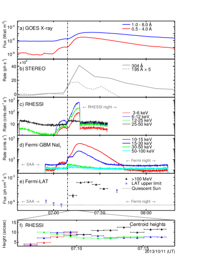
Figure 1.— Light curves of the 2013 October 11 flare as detected by a) GOES, b) STEREO, c) RHESSI, d) GBM, e) LAT, and heights of the RHESSI emission centroid (f) with the same color coding as in c). Fermi exited the South Atlantic Anomaly (SAA) at 06:57:00 UT. The vertical dashed line represents flare start time (7:01 UT).

2.2. Data analysis

We performed an unbinned likelihood analysis of the LAT data with the gtlike program distributed with the Fermi ScienceTools For RHESSI data, we applied the CLEAN imaging algorithm (Hurford et al., 2002) using the detectors 3$-$9 to reconstruct the X-ray images. We used the FITS World Coordinate System software package (Thompson & Wei, 2010) to co-register the flare location between STEREO and SDO images. The STEREO light curves are pre-flare background subtracted, full-Sun integrated photon rates.

2.3. Localization of the Emission

We measure the location of the LAT $>$100 MeV gamma-ray emission (as described in Ajello et al., 2014) and find a best fit position for the emission centroid at heliocentric coordinates of ($-850\arcsec$,$70\arcsec$) with a 68% error radius of 250$\arcsec$, as shown in Figure 2(b). RHESSI X-ray sources integrated over 07:11:04$-$07:16:44 UT are shown as 80%-level, off-limb contours in Figure 2(d).

The temporal evolution of the projected RHESSI source heights above the solar limb are shown in Figure 1(f). The higher-energy emission generally comes from greater heights, consistent with expectations for a loop-top source (e.g., Sui & Holman, 2003; Liu et al., 2004). Moreover, from SDO/AIA movies we find no signature of EUV ribbons, even in the late phase during the RHESSI night. Together, these observations provide convincing evidence that the footpoints were indeed occulted.

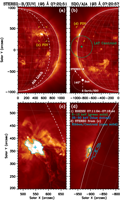
Figure 2.— STEREO-B (left) and SDO (right) images near the flare peak. The white-dashed line in (a) and (c) represents the solar limb as seen by SDO. The green line in (b) shows the 68% error circle for the LAT source centroid. The cyan contour and plus sign in (c) mark the STEREO flare ribbon and its centroid, respectively. Their projected view as seen from the AIA perspective is shown in (d), in which the centroid is located at 9^∘.9 behind the limb. The green and blue-dotted contours in (d) show RHESSI sources. The rectangular brackets in (a) and (b) mark the field of view (FOV) for (c) and (d), respectively.

The LAT measured 4 photons with energies $>$1 GeV and reconstructed direction less than 1^∘ from the center of the solar disk. All, including a 3 GeV photon, arrived after 7:19:00 UT (outside of the RHESSI coverage).

2.4. Spectral analysis

We fit the LAT gamma-ray spectral data with three models. The first two, a pure power-law (PL) and a power-law with an exponential cut-off (PLEXP) are phenomenological functions that may describe bremsstrahlung emission from accelerated electrons. The third model uses templates based on a detailed study of the gamma rays produced from pion decay (updated from Murphy et al., 1987).

We rely on the likelihood ratio test (TS; Mattox et al., 1996) to estimate the significance of the source (TS_PL) as well as to estimate whether the addition of the exponential cut-off is statistically significant. To this end we define $\Delta$TS=TS_PLEXP-TS_PL which is equivalent to the corresponding difference of maximum likelihoods computed between the two models. The significance in $\sigma$ can be roughly approximated as $\sqrt{\rm TS}$.

For each interval where PLEXP provides a significantly better fit than PL ($\Delta{\rm TS}>$20) we also fit the data with a series of pion-decay models to determine the best proton spectral index following the same procedure described in Ajello et al. (2014). The TS values for PLEXP and pion-decay fits cannot be directly compared (Wilks, 1938) however the PLEXP approximates the shape of the pion-decay spectrum (see Figure 3) thus we expect the pion-decay models to provide a similarly acceptable fit. We studied the effect of the LAT systematic uncertainties (mainly from the effective area, as considered here) via the bracketing technique described in Ackermann et al. (2012b).

The RHESSI and GBM NaI₁ spectral data are independently fitted with one or two thermal components plus a broken power-law with index fixed to 2 (to avoid energy divergence) below the break. Table 1 summarizes the spectral analysis results. Data from BGO₀ are analyzed using the procedure described in Fitzpatrick et al. (2012) with an additional 5% systematic error on the background estimation. Figure 3 shows the combined spectra from RHESSI, GBM and LAT in four integration intervals. The discrepancy (up to a factor of 2.5) between the RHESSI and GBM flux values is likely due to pile-up in the RHESSI detector, and cannot be easily corrected. As is evident from Figure 3, more energy is radiated in HXRs than gamma rays.

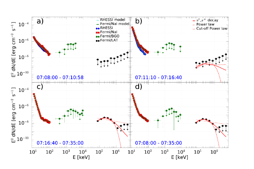
Figure 3.— Spectral energy distributions for RHESSI (blue), GBM NaI₁ (red), BGO₀ (green) and LAT (black) for four time intervals. Best fit models are shown in cyan (RHESSI), yellow (GBM) and red (LAT).

Table 1Spectral analysis of LAT, GBM and RHESSI data

LAT time intervals
Time Interval	TSPL	$\Delta$TSa	Photon index	Cutoff energyb	Proton index	Fluxc
(2013/10/11 UT)				(MeV)		($10^{-5}$ ph cm-2  s-1)
07:10:00–07:15:00	16	5	1.80$\pm$0.35${}^{+0.02}_{-0.02}$d	–	–	0.60$\pm$0.26${}^{+0.05}_{-0.04}$
07:15:00–07:20:00	987	22	0.21$\pm$0.34${}^{+0.16}_{-0.14}$	145$\pm$27${}^{+9}_{-8}$	3.7$\pm$0.2$\pm$0.1	24.1$\pm$1.5${}^{+1.6}_{-1.4}$
07:20:00–07:25:00	1146	92	0.23$\pm$0.27${}^{+0.11}_{-0.11}$	162$\pm$26${}^{+7}_{-7}$	3.5$\pm$0.2$\pm$0.1	28.2$\pm$1.7${}^{+1.7}_{-1.5}$
07:25:00–07:30:00	435	45	-0.42$\pm$0.58${}^{+0.14}_{-0.15}$	95$\pm$21${}^{+4}_{-4}$	4.3$\pm$0.4$\pm$0.1	13.7$\pm$1.33${}^{+0.8}_{-0.7}$
07:30:00–07:35:00	55	4	2.36$\pm$0.24${}^{+0.03}_{-0.02}$d	–	–	4.1$\pm$1.1${}^{+0.4}_{-0.3}$
07:08:00– 07:35:00	2885	233	0.2$\pm$0.2${}^{+0.135}_{-0.132}$	147$\pm$15${}^{+1}_{-3}$	3.7$\pm$0.2${}^{+0.1}_{-0.1}$	14.2$\pm$0.5${}^{+0.9}_{-1.2}$
07:16:40– 07:35:00	2855	204	0.4$\pm$0.2${}^{+0.134}_{-0.128}$	155$\pm$16${}^{+1}_{-2}$	3.8$\pm$0.2${}^{+0.1}_{-0.1}$	22.1$\pm$0.8${}^{+1.5}_{-1.8}$
RHESSI and GBM time intervals
		Broken power law		1st thermal component	2nd thermal component
		Ebreak	Index	Plasma temperature	Plasma temperature	Fluxe
		(keV)		(keV)	(keV)	(ph cm-2 s-1)
07:08:00–07:10:58⋆		17.9$\pm$0.5	3.76$\pm$0.04	2.23$\pm$0.06	–	52$\pm$1
07:08:00–07:10:58		17.9$\pm$0.9	3.88$\pm$0.03	1.9$\pm$0.1	–	55$\pm$1
07:11:10–07:16:40⋆		16$\pm$2	4.24$\pm$0.07	1.92$\pm$0.02	0.62$\pm$0.03	253$\pm$5
07:11:10–07:16:40		21$\pm$5	3.52$\pm$0.05	2.9$\pm$0.4	1.54$\pm$0.16	630$\pm$10
07:16:40–07:35:00		20 (fixed)	2.56$\pm$0.06	2.71$\pm$0.07	1.27$\pm$0.04	399$\pm$8
07:08:00–07:35:00		20$\pm$8	3.22$\pm$0.05	2.8$\pm$0.2	1.34$\pm$0.08	388$\pm$8

3. Discussion

We have analyzed the data of the 2013 October 11 solar flare from Fermi, RHESSI, SDO and STEREO. STEREO-B images indicate that the flare occurred in an AR 9^∘.9 behind the limb. RHESSI and GBM NaI₁ detected HXRs up to 50 keV from the flaring loop-top. The most unusual aspect of this flare is the LAT detection of photons of energies $\epsilon>$100 MeV for about 30 minutes with some photons having energies up to 3 GeV. Electrons or protons with energies $E>\epsilon$ can produce these photons after traversing a column depth of matter $N(E)>10^{25}$ and $10^{26}$ cm^-2, respectively, which is much larger than the depth $\sim 10^{20}$ cm^-2 penetrated by HXR-producing electrons. For occulted flares the emitted photons must traverse even larger depths where they may be scattered and absorbed. We consider three scenarios for the emission site of the gamma rays; (i) deep below the photosphere of the flare site (ii) in the corona above the limb, suggestive of trapping of particles, e.g., by strongly converging magnetic fields and (iii) CME-shock accelerated particles traveling back to the Sun.

3.1. Emission below the photosphere

For the first scenario we need continuous acceleration of particles because they penetrate deep into the solar atmosphere and lose energy in a fraction of a second. Most of the radiation they produce also comes from deep within the photosphere so we need to calculate the optical depth, $\tau(\epsilon)=\sigma\times N_{\gamma}(\epsilon)$ from the emission site to the Earth. For $>$100 MeV photons the main absorption is via pair production with a cross section $\sigma_{\rm PP}\sim 0.035\times\sigma_{0}$, where $\sigma_{0}$ is the Thomson scattering cross section relevant for $<$100 keV HXRs. The column depth along the line of sight to the observer, $N_{\gamma}(\epsilon)$, depends on both the position of the flare and the column depth $N(E)$ penetrated by the emitting particles of energy $E=\eta\epsilon$. This depth is determined by the energy loss rates.

High-energy electrons spiraling down a magnetic field line with a pitch angle cosine $\mu$ lose and radiate most of their energy deep in the photosphere. For $E\lesssim$ 250 MeV (Lorentz factor $\gamma\lesssim 500$), the dominant energy losses are due to Coulomb-ionization, whereas for $E\gtrsim$ 250 MeV, the radiative losses are dominated by bremsstrahlung (over synchrotron and inverse Compton). The total loss rate can be approximated as

$$dE/dr=(1/\mu)m_{e}c^{2}(n/N_{0})[1+(\gamma/\gamma_{0})^{\delta}]$$ (1)

with $N_{0}=(4\pi r_{0}^{2}\ln\Lambda)^{-1}=5\times 10^{22}\,{\rm cm}^{-2}$ (for Coulomb logarithm $\ln\Lambda=20$) and $n$ the total density. For extreme relativistic electrons $\delta\sim 1.1$ and $\gamma_{0}$ is the Lorentz factor where the two losses are equal. From these, and ignoring the small deviation of $\delta$ from unity, the column depth penetrated by an electron of initial Lorentz factor $\gamma$ is then

$$N(E)=\int_{R}^{\infty}n(r)dr=\mu N_{0}\gamma_{0}\ln(1+\gamma/\gamma_{0}).$$ (2)

For non-relativistic electrons and protons the Coulomb collision dominates and for both particles we have

$$N(E)=\mu N_{0}(m/m_{e})(E/mc^{2})^{2}/\gamma.$$ (3)

The energy dependence of the proton loss rate is similar to that of electrons. The Coulomb losses dominate at low energies but for proton energies $E>0.3$ GeV pion production becomes significant and at $E>4.5$ GeV ($\gamma\gtrsim 4$) it becomes the dominant loss mechanism, and like electron bremsstrahlung, it gives $dE/ds\propto\gamma\ln\gamma$. Making the same approximation as above we get the same equations, (1) and (2), but now with $N_{0}=6\times 10^{25}$cm^-2 and $\gamma_{0}=4.0$ (for $\ln\Lambda=30$).

An electron of energy $E$ radiates photons of energy ${\bar{\epsilon}}=E/\eta<E$ with $\eta\sim 2$. Similarly, assuming that protons of energy $E$ produce a $\pi^{0}$ with similar energy that decays into two photons of equal energies we can again set $\eta\sim 2$ (the exact value of $\eta$ will not change our conclusions drastically). For relativistic electrons the radiated photons will be beamed along the pitch angle of the electrons. As shown by McTiernan & Petrosian (1990) there will be strong center-to-limb variation of gamma-ray flux, but for flares at a few degrees behind the limb this effect can be ignored.

For a flare at the center of the solar disk (helio-longitude $\phi=0$, or angle to the limb $\theta\equiv\pi/2-\phi=\pi/2$), the optical depth is $\tau(\epsilon)=N(E=\eta\epsilon)\sigma$ and increases toward the limb at a rate that depends on the ambient density profile; $N_{\gamma}(\epsilon,\theta)=\int_{0}^{\infty}n(r)dl$, where $r=\sqrt{R^{2}+2Rl\sin\theta+l^{2}}$, and $R$ is the distance from the center of the Sun at the depth of emission $N(E)$. The photons of interest here are produced below the photosphere at column depths $N>10^{25}$ cm^-2 and densities $n>10^{17}$ cm^-3, where both quantities increase exponentially with a scale height $H\ll$ $R_{\odot}$. Consequently, most of the contribution comes from within a scale height at a radius $R\sim$ $R_{\odot}$ corresponding to the column depth $N(\eta\epsilon)$ described above. If we define $A=R/H$ and $d\lambda=dl/R$ we get

$$N_{\gamma}(\epsilon,\theta)=N(E=\eta\epsilon)Ae^{A}\int_{0}^{\infty}e^{-A\sqrt{1+2\lambda\sin\theta+\lambda^{2}}}d\lambda.$$ (4)

For occulted flares $\theta<0$. Since $A\gg 1$ most of the contribution to this integral comes from very small $\lambda$ so we can use the approximation $\sqrt{1+2\lambda\sin\theta+\lambda^{2}}\sim(1+\lambda\sin\theta+\lambda^{2}\cos^{2}(\theta)/2)$. This gives

$$N_{\gamma}(\epsilon,\pm\theta)=N(\eta\epsilon)\sqrt{\pi A/(2\cos^{2}\theta)}\,e^{\xi}\,[1\mp{\rm erf}(\sqrt{\xi})],$$ (5)

where $\xi\equiv A\tan^{2}(\theta)/2$. Thus, we get $N_{\gamma}(\epsilon,\pi/2)=N(\eta\epsilon)$ and $N_{\gamma}(\epsilon,0)=N(\eta\epsilon)\sqrt{\pi A/2}$ for flares at the center and limb of the Sun. However, we are interested in behind-the-limb flares with $|\theta|\ll 1$ so that $\xi\equiv\theta^{2}A/2=0.1(\theta^{\circ})^{2}(10^{3}\,{\rm km/H})$. For angles $|\theta|>3^{\circ}$ the error functions ${\rm erf}(\sqrt{\xi})\rightarrow 1$ and $N_{\gamma}(\epsilon,-\theta)=2N(\eta\epsilon)\sqrt{\pi A/2}e^{\xi}$.

We can use these expressions to calculate the optical depth. Let us consider HXRs emitted by nonrelativistic electrons. For a 50 keV photon emitted by a $\mu=0.5$ and $E=100$ keV electron (and using the Thomson cross section) we find $\tau(50\,{\rm keV},\theta=\pi/2)<10^{-3}$ at the center of the disk, $\tau(50\,{\rm keV},\theta=0)\sim 0.02$ at the limb, and a rapid increase as $e^{0.1\theta^{2}}$ for a behind-the-limb flare. At $\theta=-10$^∘ and $H=1000$ km, the optical depth is $\gtrsim 10^{3}$.

For gamma rays the optical depth is considerably larger because they are emitted deeper in the photosphere. For a flare near the center of the solar disk the optical depth for a 100 MeV photon, emitted either by a $\sim 200$ MeV electron or $>350$ MeV proton, is about 0.2 and 0.1, respectively. But for a flare at the limb these values increase by $\sqrt{\pi A/2}=33\times(10^{3}\,{\rm km/H})^{1/2}$. For reasonable average pitch angles ${\bar{\mu}}>0.1$ and even if we include the effects of non-radial field lines this could give $\tau>1$.

Once the flare source region moves behind the limb, the optical depth increases exponentially as $e^{\xi}\propto e^{\theta^{2}A/2}$ making the detection of any flare for $|\theta|>2$^∘ impossible. This is also true for the 1 to 10 MeV BGO photons even though the protons producing them do not penetrate as deeply. Considering that the flare occurred at $\sim$10^∘ behind the limb, we conclude that this scenario is untenable.

3.2. Emission in the corona

The key feature of this behind-the-limb flare is the detection of $>$100 MeV emission for $\sim$30 minutes. To explain this observation, we also consider the scenario where the photons are produced in the corona by high-energy particles injected promptly into a magnetic trap (e.g., Aschwanden et al., 1997) at $>10^{9}$ cm ( minimum height needed for a source $\sim$10^∘ behind the limb to be visible above the limb) above the transition region. For particles to be trapped efficiently we need sufficiently strong field convergence to trap most particles and a low level of turbulence so that the scattering time would be much longer than the energy loss time. Otherwise most of the particles will be scattered into the loss cone and radiate deep in the solar atmosphere as in scenario 3.1.

Let us first consider protons with an energy loss rate given by Eq. (1) with $\delta=1,N_{0}=6\times 10^{25}$ cm^-2 and $\gamma_{0}=4.0$. This gives an energy loss time for a 1 GeV proton of $\tau_{0}\sim 2\times 10^{15}\,{\rm s\cdot cm}^{-3}/n$ so for the observed duration of $<2000$ s we need a density $n>10^{12}\,{\rm cm}^{-3}$ which is what one encounters below the occulted transition region and not at $>10^{9}$ cm above it. The energy loss rate for electrons in the coronal region is dominated by Coulomb collisions at low energies and synchrotron losses for magnetic fields $B>10$ G or inverse Compton losses at lower fields. This rate is again described by Eq. (1) but with $\delta=2,N_{0}=5\times 10^{22}$ cm^-2 and $\gamma_{0}=21.5\times(n/10^{10}~{}{\rm cm}^{-3})^{1/2}\times(B/100~{}{\rm G})^{-1}$. As shown in Petrosian (2001), this gives rise to flat spectra at low energies and a sharp cutoff at $\gamma\sim\gamma_{0}$ with these electrons carrying most of the energy with the longest lifetime of $\tau_{0}\sim\gamma_{0}N_{0}/(2nc)$. For the production of $>100$ MeV photons we need electrons with $\gamma_{0}\sim 300$ so that for a lifetime of 30 minutes we need $n\sim 10^{11}\,{\rm cm}^{-3}$ and $B\sim$ 25 G. While these values for the density (magnetic field) are somewhat higher (lower) than the ones found at 10⁹ cm above the transition region, they cannot be fully ruled out. Also, a photon index $\Gamma\sim 0$ requires injected electrons with spectral index -1 (for a thin target case), which is much harder than those encountered at lower energies. Thus, this model requires strong convergence, low turbulence and hard spectra. In view of the LAT detection of SOL2014-09-01 flare with $\theta\sim 36^{\circ}$ (paper in preparation) that requires a trap at a height $>$10¹⁰ cm, this model becomes less plausible.

3.3. Acceleration in CME Shocks

A third possibility is that particles accelerated by a shock associated with this flare originating behind the limb find their way to the photosphere visible to Fermi where they produce gamma-rays. This requires a magnetic connection between the acceleration site and the visible photosphere, e.g., large overlying loops. Such a connection must have been absent during the impulsive phase and for HXR-producing electrons which are most likely accelerated in smaller loops with both footpoints occulted. Otherwise we would expect a detection of HXRs from the footpoints on the visible side. Furthermore, the LAT emission error circle allows for the gamma-ray emission to occur on the visible side of the disk. This also means that the extended-phase gamma-ray producing particles were not accelerated in small loops and, like longer lasting SEPs, most likely were accelerated in the shock of the CME. Since the magnetic lines draping the CME are most likely connected to the occulted AR, this requires cross-field diffusion that allows migration of particles from the field lines connected to the AR to those connected to the visible disk. The presence of a strong and short scale turbulence capable of scattering the accelerated particles with a mean free path comparable to their gyro radii will facilitate this migration (Zhang et al., 2003). A longer trapping time of accelerated particles in the downstream region, say e.g., by converging field lines rooted at the Sun, can also help this migration. This model requires further study.

In conclusion, the multiwavelength observations of this behind-the-limb flare have provided some interesting theoretical puzzles which can be resolved by more detailed investigation of the scenarios discussed above.

References

- Ackermann et al. (2012a) Ackermann, M., Ajello, M., Allafort, A., et al. 2012a, ApJ, 745, 144
- Ackermann et al. (2012b) Ackermann, M., Ajello, M., Albert, A., et al. 2012b, ApJS, 203, 4
- Ackermann et al. (2014) Ackermann, M., Ajello, M., Albert, A., et al. 2014, The Astrophysical Journal, 787, 15
- Ajello et al. (2014) Ajello, M. A. A., Allafort, A., Baldini, L., et al. 2014, The Astrophysical Journal, 789, 20
- Aschwanden et al. (1997) Aschwanden, M. J., Bynum, R. M., Kosugi, T., Hudson, H. S., & Schwartz, R. A. 1997, ApJ, 487, 936
- Atwood et al. (2009) Atwood, W. B.Abdo, A. A., Ackermann, M., Ajello, M., et al. 2009, ApJ, 697, 1071
- Barat et al. (1994) Barat, C., Trottet, G., Vilmer, N., et al. 1994, ApJ, 425, L109
- Fitzpatrick et al. (2012) Fitzpatrick, G., McBreen, S., Connaughton, V., & Briggs, M. 2012, in Society of Photo-Optical Instrumentation Engineers (SPIE) Conference Series, Vol. 8443, Society of Photo-Optical Instrumentation Engineers (SPIE) Conference Series, 3
- Fletcher & Hudson (2008) Fletcher, L., & Hudson, H. S. 2008, ApJ, 675, 1645
- Forrest et al. (1985) Forrest, D. J., Vestrand, W. T., Chupp, E. L., et al. 1985, International Cosmic Ray Conference, 4, 146
- Haerendel (2012) Haerendel, G. 2012, ApJ, 749, 166
- Holman et al. (2011) Holman, G. D., Aschwanden, M. J., Aurass, H., et al. 2011, Space Sci. Rev., 159, 107
- Hoyng et al. (1981) Hoyng, P., Duijveman, A., Machado, M. E., et al. 1981, ApJ, 246, L155
- Hurford et al. (2002) Hurford, G. J., Schmahl, E. J., Schwartz, R. A., et al. 2002, Solar Physics, 210, 61
- Krucker & Lin (2008) Krucker, S., & Lin, R. P. 2008, ApJ, 673, 1181
- Krucker et al. (2007) Krucker, S., White, S. M., & Lin, R. P. 2007, ApJ, 669, L49
- Kuznetsov et al. (2011) Kuznetsov, S., Kurt, V., Yushkov, B., Kudela, K., & Galkin, V. 2011, Solar Physics, 268, 175
- Lemen et al. (2012) Lemen, J., Title, A., Akin, D., et al. 2012, Solar Physics, 275, 17
- Liu et al. (2013) Liu, W., Chen, Q., & Petrosian, V. 2013, ApJ, 767, 168
- Liu et al. (2004) Liu, W., Jiang, Y. W., Liu, S., & Petrosian, V. 2004, ApJ, 611, L53
- Liu et al. (2008) Liu, W., Petrosian, V., Dennis, B. R., & Jiang, Y. W. 2008, ApJ, 676, 704
- Martínez Oliveros et al. (2012) Martínez Oliveros, J.-C., Hudson, H. S., Hurford, G. J., et al. 2012, ApJ, 753, L26
- Masuda et al. (1994) Masuda, S., Kosugi, T., Hara, H., Tsuneta, S., & Ogawara, Y. 1994, Nature, 371, 495
- Mattox et al. (1996) Mattox, J. R., Bertsch, D. L., Chiang, J., et al. 1996, ApJv.461, 461, 396
- McTiernan & Petrosian (1990) McTiernan, J. M., & Petrosian, V. 1990, ApJ, 359, 541
- Meegan et al. (2009) Meegan, C., Lichti, G., Bhat, P. N., et al. 2009, ApJ, 702, 791
- Murphy et al. (1987) Murphy, R. J., Dermer, C. D., & Ramaty, R. 1987, ApJS, 63, 721
- Nitta et al. (2013) Nitta, N. V., Aschwanden, M. J., Boerner, P. F., et al. 2013, Sol. Phys., 288, 241
- Petrosian (2001) Petrosian, V. 2001, ApJ, 557, 560
- Petrosian et al. (2002) Petrosian, V., Donaghy, T. Q., & McTiernan, J. M. 2002, ApJ, 569, 459
- Petrosian et al. (1994) Petrosian, V., McTiernan, J. M., & Marschhauser, H. 1994, ApJ, 434, 747
- SOHO LASCO CME CATALOG (2013) SOHO LASCO CME CATALOG. 2013, http://cdaw.gsfc.nasa.gov/CME_list/
- Sui & Holman (2003) Sui, L., & Holman, G. D. 2003, ApJ, 596, L251
- Thompson et al. (1993) Thompson, D. J., Bertsch, D. L., Fichtel, C. E., et al. 1993, ApJS, 86, 629
- Thompson & Wei (2010) Thompson, W. T., & Wei, K. 2010, Sol. Phys., 261, 215
- Vestrand & Forrest (1993) Vestrand, W. T., & Forrest, D. J. 1993, ApJ, 409, L69
- Vilmer et al. (1999) Vilmer, N., Trottet, G., Barat, C., et al. 1999, A&A, 342, 575
- Wilks (1938) Wilks, S. S. 1938, Ann. Math. Stat., 9, 60
- Wuelser et al. (2004) Wuelser, J., Lemen, J. R., Tarbell, T. D., et al. 2004, Society of Photo-Optical Instrumentation Engineers (SPIE) Conference Series 5171 (2004)
- Zhang et al. (2003) Zhang, M., Jokipii, J. R., & McKibben, R. B. 2003, ApJ, 595, 493