Sub-Nanosecond Time of Flight on Commercial Wi-Fi Cards

Abstract

Time-of-flight, i.e., the time incurred by a signal to travel from transmitter to receiver, is perhaps the most intuitive way to measure distances using wireless signals. It is used in major positioning systems such as GPS, RADAR, and SONAR. However, attempts at using time-of-flight for indoor localization have failed to deliver acceptable accuracy due to fundamental limitations in measuring time on Wi-Fi and other RF consumer technologies. While the research community has developed alternatives for RF-based indoor localization that do not require time-of-flight, those approaches have their own limitations that hamper their use in practice. In particular, many existing approaches need receivers with large antenna arrays while commercial Wi-Fi nodes have two or three antennas. Other systems require fingerprinting the environment to create signal maps. More fundamentally, none of these methods support indoor positioning between a pair of Wi-Fi devices without third party support.

In this paper, we present a set of algorithms that measure the time-of-flight to sub-nanosecond accuracy on commercial Wi-Fi cards. We implement these algorithms and demonstrate a system that achieves accurate device-to-device localization, i.e. enables a pair of Wi-Fi devices to locate each other without any support from the infrastructure, not even the location of the access points.

1 Introduction

The time-of-flight of a signal captures the time it takes to propagate from a transmitter to a receiver. Time-of-flight is perhaps the most intuitive method for localization using wireless signals. If one can accurately measure the time-of-flight from a transmitter, one can compute the transmitter’s distance simply by multiplying the time-of-flight by the speed of light. As early as World War I, SONAR systems used the time-of-flight of acoustic signals to localize submarines. Today, GPS, the most widely used outdoor localization system, localizes a device using the time-of-flight of radio signals from satellites. However, applying the same concept to indoor localization has proven difficult. Systems for localization in indoor spaces are expected to deliver high accuracy (e.g., a meter or less) using consumer-oriented technologies (e.g., Wi-Fi on one’s cellphone). Unfortunately, past work could not measure time-of-flight at such an accuracy on Wi-Fi devices [55, 10]. As a result, over the years, research on accurate indoor positioning has moved towards more complex alternatives such as employing large multi-antenna arrays to compute the angle-of-arrival of the signal [56, 30]. These new techniques have delivered highly accurate indoor localization systems.

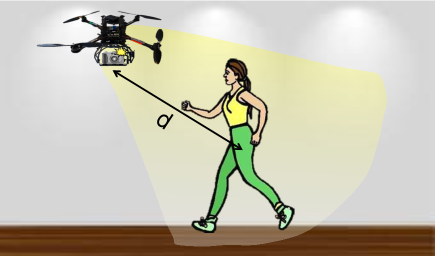
Figure 1: Chronos on a personal drone: Chronos enables a drone to maintain a safe distance $d$ from a user by tracking a device in her pocket, while capturing a video in uncalibrated indoor environments.

Despite these advances, time-of-flight based localization has some of the basic desirable features that state-of-the-art indoor localization systems lack. In particular, measuring time-of-flight does not require more than a single antenna on the receiver. In fact, by measuring time-of-flight of a signal to just two antennas, a receiver can intersect the corresponding distances to locate its source. In other words, a receiver can locate a wireless transmitter with no support from surrounding infrastructure whatsoever. This is quite unlike current indoor localization systems, which require the help of multiple access points to find the distance between a pair of mobile devices. Furthermore, each of these access points need to have many antennas – far beyond what is supported in commercial Wi-Fi devices. In addition, the location of these access points has to be calibrated and known a priori.

But, why is it that one cannot accurately measure time-of-flight on commercial Wi-Fi devices in the first place? In particular, to achieve state-of-the-art positioning accuracy, one must measure time-of-flight at sub-nanosecond granularity. However, doing so on commercial Wi-Fi cards is fundamentally challenging for the following three reasons.

Limited Time Granularity: First, the straightforward approach to measure time-of-flight is to read off the clock of the Wi-Fi radio when the signal arrives [55]. Unfortunately, the clocks on today’s Wi-Fi cards operate at tens of Megahertz, limiting their resolution in measuring time to tens of nanoseconds [10, 49, 40]. To put this in perspective, a clock running at 20 MHz (the bandwidth of typical Wi-Fi systems), can only tell apart distances separated by 15 m, making it impractical for accurate indoor positioning. Even recent state-of-the-art systems that measure time-of-flight using high-resolution 88 MHz Wi-Fi clocks [39] and super-resolution channel processing techniques [57] suffer a mean localization error of about 2.3 m.

Packet Detection Delay: Second, any measurement of time-of-flight of a packet necessarily includes the delay in detecting its presence. To make matters worse, this packet detection delay is typically orders-of-magnitude higher than time-of-flight. For indoor Wi-Fi environments, time-of-flight is just a few nanoseconds, while packet detection delay spans hundreds of nanoseconds [45]. Today, there is no way to tease apart the time-of-flight from this detection delay.

Multipath: Finally, in indoor environments, signals do not experience a single time-of-flight, but a time-of-flight spread. To see why, observe that wireless signals in indoor environments travel along multiple paths, and bounce off walls and furniture. As a result, the receiver obtains several copies of the signal, each having experienced a different time-of-flight. To perform accurate localization, one must therefore be able to disentangle the time-of-flight of the most direct path from all the remaining paths.

In this paper, we show that it is possible to design algorithms that overcome the above limitations and measure the time-of-flight at sub-nanosecond accuracy using off-the-shelf Wi-Fi cards. At a high level, our approach is based on the following observation: If one had a very wideband radio (e.g., a few GHz), one could measure time of flight at sub-nanosecond accuracy. While each Wi-Fi frequency band is only tens of Megahertz wide, there are many such bands that together span a very wide bandwidth. Our solution therefore collects measurements on multiple Wi-Fi frequency bands and stitches them together to give the illusion of a wide-band radio. Our key contribution is an algorithm that achieves this, despite the fact that Wi-Fi frequency bands are non-contiguous, and in some cases, a few Gigahertz apart. We further develop a set of algorithms that build on this idea to overcome each of the aforementioned challenges. We also detail the benefits and limitations of such a design.

To demonstrate the performance and practicality of our design, we built Chronos, a software-only solution that harnesses our algorithms to enable a pair of commercial Wi-Fi devices to locate each other without any support from the infrastructure. To illustrate its capabilities, we apply Chronos to personal drones [43] that follow a user around and capture videos of their everyday indoors activities. Such drones can help monitor fitness, activities and exercise of users at home, work or the gym (see Fig. 1). Chronos allows a personal drone to maintain the best possible distance relative to its user to take optimal videos at the right focus. It achieves this by using the Wi-Fi card on the drone to locate the user’s device, without any help from the infrastructure. The application also illustrates Chronos’s ability to run on standard 3-antenna Wi-Fi cards, as opposed to large antenna arrays, which would be too heavy and difficult to mount on lightweight indoor drones.

We evaluated Chronos’s performance on pairs of devices equipped with Intel 5300 Wi-Fi cards, including Thinkpad W530 laptops, as well as an AscTec Atom board (a small computing board) mounted on an AscTec Hummingbird Quadrotor drone platform. Our results reveal the following:

• Chronos achieves a median error in time-of-flight of 0.47 ns in line-of-sight and 0.69 ns in non-line-of-sight settings, corresponding to a physical distance accuracy of 14.1  cm and 20.7  cm respectively.

• Chronos uses time-of-flight to triangulate the location of the device with a median error of 58 cm in line-of-sight and 118 cm in non-line-of-sight settings.

• When mounted on a drone, Chronos integrates with robotic control algorithms to further improve its accuracy. It maintains the required distance relative to a user’s device with a root mean-squared error of 4.2 cm.

Contributions: To our knowledge, Chronos is the first RF-based positioning system that can measure sub-nanosecond time of flight on commercial Wi-Fi cards. Chronos leverages the time-of-flight measurements to estimate device-to-device distance measurements without any infrastructure support. Finally, Chronos operates on typical 2/3-antenna Wi-Fi receivers, yet delivers state-of-the-art localization accuracy.

2 Related Work

This paper is closely related to past work that measures the time-of-flight of Wi-Fi signals. There have been several studies that resolve time-of-flight to around ten nanoseconds using the clocks of Wi-Fi cards [55, 35, 19, 38]. Many conclude that the clocks on current Wi-Fi hardware alone cannot permit higher resolutions of time-of-flight [10, 49, 40]. Some systems have attempted to compensate for the lack of accurate time-of-flight measurements on Wi-Fi radios by augmenting their designs with other sensors and hardware. In particular, SAIL [39] couples time-of-arrival measurements on the 88 MHz clock of an Atheros Wi-Fi card with inertial motion sensors on a mobile device. It asks the user to physically walk to different locations and couples Wi-Fi channel measurements at a single access point with readings of motion sensors on their mobile device. SAIL processes this information to measure time-of-flight at a granularity of several nanoseconds, achieving localization accuracy of a few meters. However, unlike Chronos, SAIL requires users to physically move to different locations, along restricted classes of trajectories, due to its reliance on motion sensors. Synchronicity [57] uses three WARP access points to compute the location of a Wi-Fi transmitter using their time-difference of arrival. Synchronicity requires the different access points to be synchronized in time. The authors achieve this in their current implementation by connecting the access points to the same reference clock, and leave distributed time-synchronization for future work. We believe Chronos coupled with SourceSync [45] can complement Synchronicity by maintaining accurate time-synchronization between access points, while accounting for their relative time-of-flight. Finally recent theoretical work [54, 48] has proposed using a single large 8-antenna array to measure time-of-flight for indoor positioning. Unlike Chronos, these papers assume time and frequency synchronization of the access point and client, which is hard to ensure in practice [46].

Our work is also related to other RF-based indoor localization solutions. Such systems measure metrics other than time-of-flight, like angle-of-arrival and received signal power, across many RF receivers in the environment. Some achieve this using advanced infrastructure such as antenna arrays [30, 56, 53]. Others rely on a combination of fingerprinting of the environment and modeling received signal power at multiple client locations using multiple access points in the environment [47, 12, 8, 58]. Recent work requires neither [34, 20], but assumes the presence of multiple Wi-Fi access points in the environment. Unlike these systems, Chronos infers location between a single pair of commodity Wi-Fi devices, without requiring prior fingerprinting of the environment or support of the infrastructure.

This paper is related to past systems on time-synchronization. For example, SourceSync [45] and FICA [15] measure time-of-arrival to synchronize the transmissions of distributed access points. However, these systems mainly focus on estimating time-of-arrival as opposed to time-of-flight, which is dominated by packet detection delay, as we show in §5. In contrast, Chronos directly measures time-of-flight at a sub-nanosecond granularity, bereft of packet detection delay, and can therefore complement these systems to further improve their accuracy.

Finally, our work relates to past non-Wi-Fi localization systems, some measuring time-of-flight, e.g. ultra-wideband [32], pulse radar [18], acoustic systems [51, 37], device-free localization systems [4, 44, 42], vision-based systems [33, 5, 16] and inertial-measurement based systems [36, 50]. These systems either deploy custom infrastructure [51, 18], assume special markers in the environment [41], or suffer from poor accuracy [50]. In contrast, Chronos can leverage existing Wi-Fi radios that are ubiquitous in today’s mobile devices, laptops and access points.

3 Overview of Chronos

This section briefly outlines Chronos’s key challenges. Chronos’s core contribution is a new method that computes time of flight of a Wi-Fi signal. However, as mentioned in the introduction, obtaining highly accurate time-of-flight on Wi-Fi devices requires addressing three main challenges:

• Limited Time Granularity: First, Chronos needs to compute accurate time-of-flight despite the limited clock resolution of commercial Wi-Fi cards (See §4).

• Eliminating Packet Detection Delay: Second, it must disentangle time-of-flight from packet detection delay, which is often orders-of-magnitude larger (See §5).

• Combating Multipath: Third, Chronos should separate the time-of-flight of direct path of the wireless signal from that of all the remaining paths (See §6).

In the following sections, we describe how Chronos overcomes each of the above challenges as well as other practical issues to enable a robust system design.

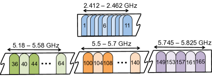
Figure 2: Wi-Fi Bands: Depicts Wi-Fi bands at 2.4 GHz and 5 GHz. Note that some of these frequencies (e.g. 5.5-5.7 GHz) are DFS bands in the U.S. that many 802.11h compatible 802.11n radios like Intel 5300 support.

4 Measuring Time of Flight

In this section, we describe how Chronos measures accurate time-of-flight of received signals, despite the limited time resolution of commodity Wi-Fi devices. For clarity, the rest of this section assumes signals propagate from the transmitter to a receiver along a single path with no detection delay. We address challenges stemming from packet detection delay and multipath in §5 and §6 respectively.

Chronos’s approach is based on the following observation: Conceptually, if our receiver had a very wide bandwidth, it could readily measure time-of-flight at a fine-grained resolution. Unfortunately, today’s Wi-Fi devices do not have such wide bandwidth. But there is another opportunity: Wi-Fi devices are known to span multiple frequency bands scattered around 2.4 GHz and 5 GHz. Combined, these bands span almost one GHz of bandwidth. By making a transmitter and receiver hop between these different frequency bands, we can gather many different measurements of the wireless channel. We can then “stitch together” these measurements to compute the time-of-flight, as if we had a very wideband radio.

While channel hopping provides the intuition on how to compute accurate time-of-flight, transforming this idea into practice is not simple. Our method must account for the fact that many Wi-Fi bands are non-contiguous, unequally spaced, and even multiple GHz apart (see Fig. 2).

Chronos’s solution to overcome these challenges exploits the phase of wireless channels. Specifically, we know from basic electromagnetics that as a signal propagates in time, it accumulates a corresponding phase depending on its frequency. The higher the frequency of the signal, the faster the phase accumulates. To illustrate, let us consider a transmitter sending a signal to its receiver. Then we can write the wireless channel $h$ as [52]:

$$h=ae^{-j2\pi f\tau}$$ (1)

Where $a$ is the signal magnitude that captures its attenuation over the air, $f$ is the frequency and $\tau$ is the time-of-flight. The phase of this channel depends on time-of-flight as:

$$\angle h=-2\pi f\tau\mod 2\pi$$ (2)

Notice that the above equation depends directly on the signal’s time-of-flight. In other words, it does not depend on the signal’s precise time-of-departure at the transmitter. Hence, we can use Eqn. 2 above to measure the time-of-flight $\tau$ as:

$$\tau=-\frac{\angle h}{2\pi f}\mod\frac{1}{f}$$ (3)

The above equation gives us the time-of-flight modulo ${1}/{f}$. Hence, for a Wi-Fi frequency of $2.4$ GHz, we can only obtain the time-of-flight modulo $0.4$ nanoseconds. Said differently, transmitters with times-of-flight $0.1$ ns, $0.5$ ns, $0.9$ ns, $1.3$ ns, etc. all produce identical phase in the wireless channel. In terms of physical distances, this means transmitters at distances separated by multiples of $12$ cm (e.g., $3$ cm, $15$ cm, $27$ cm, $39$ cm, etc.) all result in the same channel phase. Consequently, there is no way to distinguish between these transmitters using their phase on a single channel.

Indeed, this is precisely why Chronos needs to hop between multiple frequency bands $\{f_{1},\dots,f_{n}\}$ and measure the corresponding wireless channels $\{h_{1},\dots,h_{n}\}$. The result is a system of equations, one per frequency, that measure the time-of-flight modulo different values:

$$\tau= -\frac{\angle h_{1}}{2\pi f_{1}}\mod\frac{1}{f_{1}}$$

$$\tau= -\frac{\angle h_{2}}{2\pi f_{2}}\mod\frac{1}{f_{2}}$$

$$\vdots$$

$$\tau= -\frac{\angle h_{n}}{2\pi f_{n}}\mod\frac{1}{f_{n}}$$ (4)

Notice that the above set of equations has the form of the well-known Chinese remainder theorem [24]. Such equations can be readily solved using standard modular arithmetic algorithms, even amidst noise [13]. The theorem states that solutions to these equations are unique modulo a much larger quantity – the Least Common Multiple (LCM) of $\{{1}/{f_{1}},\dots,{1}/{f_{n}}\}$. For instance, Chronos can resolve time-of-flight uniquely modulo 200 ns using Wi-Fi frequency bands around 2.4 GHz. That is, it can resolve transmitters closer than $60~{}\text{m}$ in distance without ambiguity, which is sufficient for most indoor environments.

To illustrate how the above system of equations works, consider a source at 0.6 m whose time-of-flight is 2 ns. Say the receiver measures the channel phases from this source on five candidate Wi-Fi channels as shown in Fig. 3. We note that a measurement on each of these channels produces a unique equation for $\tau$, like in Eqn. 4. Each equation has multiple solutions, depicted as colored vertical lines in Fig. 3. However, only the correct solution of $\tau$ will satisfy all equations. Hence, by picking the solution satisfying the most number of equations (i.e., the $\tau$ with most number of aligned lines in Fig. 3), we can recover the true time-of-flight of 2 ns.

Note that our solution based on the Chinese remainder theorem makes no assumptions on whether the set of frequencies $\{f_{1},\dots,f_{n}\}$ are equally separated or otherwise. In fact, having unequally separated frequencies makes them less likely to share common factors, boosting the LCM. This means that counter-intuitively, the scattered and unequally-separated bands of Wi-Fi (see Fig. 2) are not a challenge, but an opportunity to resolve larger values of $\tau$.

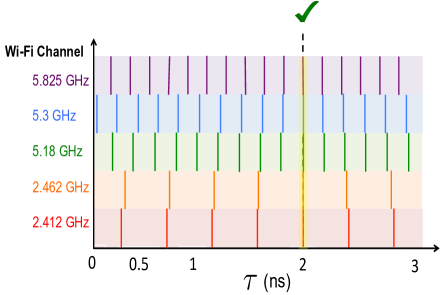
Figure 3: Measuring Time-of-Flight: Consider a wireless transmitter at a distance of $0.6$ m, i.e. a time-of-flight of $2$ ns. The phase of each Wi-Fi channel results in multiple solutions, depicted as colored lines, including $2$ ns. However, the solution that satisfies most equations, i.e. has the most number of aligned colored lines is the true time-of-flight ($2$ ns).

While the above provides a mathematical formulation of our algorithm, we describe below important systems considerations in applying Chronos to commercial Wi-Fi cards:

• Chronos must ensure both the Wi-Fi transmitter and receiver hop synchronously between multiple Wi-Fi channels. Chronos achieves this using a channel hopping protocol driven by the transmitter. Before switching frequency bands (every 2-3 ms in our implementation), the transmitter issues a control packet that advertises the frequency of the next band to hop to. The receiver responds with an acknowledgment and switches to the advertised channel. Once the acknowledgment is received, the transmitter switches frequency bands as well. As a fail-safe, transmitters and receivers revert to a default frequency band if they do not receive packets or acknowledgments from each other for a given time-out duration on any band.

• Our implementation of Chronos sweeps all Wi-Fi bands in 84 ms (12 times per second). This is within the channel coherence time of indoor environments [46] and can empirically localize users at walking speeds (see §12.4).

• Chronos primarily targets device-to-device localization between two users where data is typically not exchanged. However, we discuss and evaluate the implications of Chronos’s protocol on data traffic in §10 and §12.3.

• Finally, wireless transmitters and receivers experience carrier frequency offsets (CFO). These offsets cause phase errors in measured wireless channels. §7 describes how Chronos corrects frequency offsets, and additional phase offsets from differences in transmit and receive hardware.

5 Eliminating Packet Detection Delay

Our discussion so far has computed time-of-flight based on the wireless channels $h_{i}$ that signals experience when transmitted over the air on different frequencies $f_{i}$. The phase of such channels depends exclusively on the time-of-flight of the signal, and its frequency. In practice however, the measured wireless channels at the receiver, $\tilde{h}_{i}$, experience a delay in addition to time-of-flight: the delay in detecting the presence of a packet. This delay occurs because Wi-Fi receivers detect the presence of a packet based on the energy of its first few time samples. The number of samples that the Wi-Fi receiver needs to cross its energy detection threshold varies based on the power of the received signal, as well as noise. While this variation may seem small, packet detection delays are often an order-of-magnitude larger than time-of-flight, particularly in indoor environments, where time-of-flight is just a few tens of nanoseconds (See §12.1).

Hence, our main goal here is to derive the true channel $h_{i}$ (which incorporates the time-of-flight alone) from the measured channel $\tilde{h}_{i}$ (which incorporates both time-of-flight and packet detection delay). To do this, we exploit the fact that Wi-Fi uses OFDM. Specifically, the bits of Wi-Fi packets are transmitted in the frequency domain on several small frequency bins called OFDM subcarriers. This means that the wireless channels $\tilde{h}_{i}$ can be measured on each subcarrier. We then make the following main claim: The measured channel at subcarrier-$\mathrm{\Gamma }$ does not experience packet detection delay, i.e. it is identical in phase to the true channel at subcarrier $\mathrm{\Gamma }$.

To see why this claim holds, note that while time-of-flight and packet detection delay appear very similar, they occur at different stages of a signal’s lifetime. Specifically, time-of-flight occurs while the wireless signal is transmitted over the air (i.e., in passband). In contrast, packet detection delay stems from energy detection that occurs in digital processing once the carrier frequency has been removed (in baseband). Thus, time-of-flight and packet detection delay affect the wireless OFDM channels in slightly different ways.

To understand this difference, consider a particular Wi-Fi frequency band $i$. Let $\tilde{h}_{i,k}$ be the measured channel of OFDM subcarrier $k$, at frequency $f_{i,k}$. $\tilde{h}_{i,k}$ experiences two phase rotations in different stages of the signal’s lifetime:

• A phase rotation in the air proportional to the over-the-air frequency $f_{i,k}$, just like the true wireless channel $h_{i,k}$. From Eqn. 2 in §4, this phase value for a frequency $f_{i,k}$ is:

  $$\angle h_{i,k}=-2\pi f_{i,k}\tau,$$

  where $\tau$ is the time-of-flight.

• An additional phase rotation due to packet detection after the removal of the carrier frequency. This additional phase rotation can be expressed in a similar form as:

  $$\Delta_{i,k}=-2\pi(f_{i,k}-f_{i,0})\delta_{i},$$

  where $\delta_{i}$ is the packet detection delay.

Thus, the total measured channel phase at subcarrier $k$ is:

$$\angle\tilde{h}_{i,k}= \angle h_{i,k}+\Delta_{i,k}$$ (5)

$$= {-2\pi}f_{i,k}\tau-2\pi(f_{i,k}-f_{i,0})\delta_{i}$$ (6)

Notice from the above equation that the second term $\Delta_{i,k}=-2\pi(f_{i,k}-f_{i,0})\delta_{i}=0$ at precisely $k=0$. In other words, at the zero-subcarrier of OFDM, the measured channel $\tilde{h}_{i,k}$ is identical in phase to the true channel $h_{i,k}$ over-the-air which validates our claim.

In practice, this means that we can apply the Chinese Remainder theorem as described in Eqn. 4 of §4 at the zero-subcarriers (i.e. center frequencies) of each Wi-Fi frequency band. In the U.S., Wi-Fi at 2.4 GHz and 5 GHz has a total of 35 Wi-Fi bands with independent center frequencies. Therefore, a sweep of all Wi-Fi frequency bands results in 35 independent equations like in Eqn. 4, which we can solve to recover time-of-flight.

However, one problem still needs to be addressed. So far we have used the measured channel at the zero-subcarrier of Wi-Fi bands. However, Wi-Fi transmitters do not send data on the zero-subcarrier, meaning that this channel simply cannot be measured. This is because the zero-subcarrier overlaps with DC offsets in hardware that are extremely difficult to remove [25, 2]. So how can one measure channels on zero-subcarriers if they do not even contain data?

Fortunately, Chronos can tackle this challenge by using the remaining Wi-Fi OFDM subcarriers, where signals are transmitted. Specifically, it leverages the fact that indoor wireless channels are based on physical phenomena. Hence, they are continuous over a small number of OFDM subcarriers [29]. This means that Chronos can interpolate the measured channel phase across all subcarriers to estimate the missing phase at the zero-subcarrier. Indeed, the 802.11n standard [2] measures wireless channels on as many as 30 subcarriers in each Wi-Fi band. Hence, interpolating between the channels not only helps Chronos retrieve the measured channel on the zero-subcarrier, but also provides additional resilience to noise.

To summarize, Chronos applies the following steps to account for packet detection delay: (1) It obtains the measured wireless channels on the 30 subcarriers on the 35 available Wi-Fi bands; (2) It interpolates between these subcarriers to obtain the measured channel phase on the zero-subcarriers on each of these bands, which is unaffected by packet detection delay. (3) It retrieves the time-of-flight using the resulting 35 channels.

6 Combating Multipath

So far, our discussion has assumed that a wireless signal propagates along a single direct path between its transmitter and receiver. However, indoor environments are rich in multipath, causing wireless signals to bounce off objects in the environment like walls and furniture. Fig. 4(a) illustrates an example where the signal travels along three paths from its sender to receiver. The signals on each of these paths propagate over the air incurring different time delays as well as different attenuations. The ultimate received signal is therefore the sum of these multiple signal copies, each having experienced a different propagation delay. Fig. 4(b) represents this using a multipath profile. This profile has peaks at the propagation delays of signal paths, scaled by their respective attenuations. Hence, Chronos needs a mechanism to find such a multipath profile, so as to separate the propagation delays of different signal paths. This allows it to then identify the time-of-flight as the least of these propagation delays, i.e. the delay of the most direct (shortest) path.

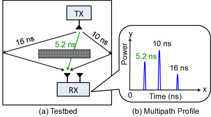
Figure 4: Combating Multipath: Consider a signal propagating from a transmitter to a receiver along three paths as shown in (a): an attenuated direct path and two reflected paths of lengths 5.2 ns, 10 ns and 16 ns respectively. These paths can be separated by using the inverse discrete Fourier transform as shown in (b). The plot has three peaks corresponding to the propagation delays of the three paths, with peak magnitudes scaled by their relative attenuations.

6.1 Computing Multipath Profiles

Let us assume that wireless signals from a transmitter reach a receiver along $p$ different paths. The received signal from each path corresponds to amplitudes $\{a_{1},\dots,a_{p}\}$ and propagation delays $\{\tau_{1},\dots,\tau_{p}\}$. Observe that our earlier Eqn. 1, considers only a single path experiencing propagation delay and attenuation. In the presence of multipath, we can extend this equation to write the measured channel $\tilde{h}_{i,0}$ on center-frequency $f_{i,0}$ as the sum of the channels on each of these paths, i.e.:

$$\tilde{h}_{i,0}=\sum_{k=1}^{p}a_{k}e^{-j2\pi f_{i,0}\tau_{k}}\text{~{}~{}~{}~{}~{}, for $i=1,\dots,n$}$$ (7)

At this point, we need to disentangle these different paths and recover their propagation delays. To do this, notice that the above equation has a familiar form – it is the well-known Discrete Fourier Transform. Thus, if one could obtain the channel measurements at many uniformly-spaced frequencies, a simple inverse-Fourier transform would separate individual paths. Such an inverse Fourier transform has a closed-form expression that can be used to obtain the propagation delay of all paths and compute the multipath profile (up to a resolution defined by the bandwidth).

Wi-Fi frequency bands, however, are not equally spaced – they are scattered around 2.4 GHz and multiple non-contiguous chunks at 5 GHz, as shown in Fig. 2. While we can measure $\tilde{h}_{i,0}$ at each Wi-Fi band, these measurements will not be at equally spaced frequencies and hence cannot be simply used to compute the inverse Fourier transform. In fact, since our measurements of the channels are not uniformly spaced, we are dealing with the Non-uniform Discrete Fourier Transform or NDFT [7]. To recover the multipath profile, we need to invert the NDFT.

6.2 Inverting the NDFT

To find the multipath profile, we must invert a Non Uniform Discrete Fourier Transform (NDFT). Computing the inverse of the NDFT is a known problem that has been studied extensively in different contexts [21, 14]. Specifically, the NDFT is an under-determined system, where the responses of multiple frequency elements are unavailable. Therefore, the inverse of such a Fourier transform no longer has a single closed-form solution, but several possible solutions. So how can Chronos pick the best among those solutions to find the true times-of-flight of the signal?

Chronos solves for the inverse-NDFT by adding a constraint to the inverse-NDFT optimization. Specifically, this constraint favors solutions that are sparse, i.e., have few dominant paths. Intuitively, this stems from the fact that while signals in indoor environments traverse several paths, a few paths tend to dominate as they suffer minimal attenuation [9]. Indeed other localization systems make this assumption as well, albeit less explicitly. For instance, antenna-array systems can resolve a limited number of dominant paths based on the number of antennas they use.

We can formulate the sparsity constraint mathematically as follows. Let the vector ${\bf p}$ sample inverse-NDFT at $m$ discrete values $\tau\in\{\tau_{1},\dots,\tau_{m}\}$. Then, we can introduce sparsity as a simple constraint in the NDFT inversion problem that minimizes the L-1 norm of ${\bf p}$. Indeed, it has been well-studied in optimization theory that minimizing the L-1 norm of a vector favors sparse solutions for that vector [6]. Thus, we can write the optimization problem to solve for the inverse-NDFT as:

$$\min \|{\bf p}\|_{1}$$ (8)

$$\text{s.t.~{}~{}~{}}\|{\bf\tilde{h}}- {\bf\mathcal{F}p}\|_{2}^{2}=0$$ (9)

where, ${\bf\mathcal{F}}$ is the $n\times m$ Fourier matrix, i.e. ${\bf\mathcal{F}}_{i,k}=e^{-j2\pi f_{i,0}\tau_{k}}$, ${\bf\tilde{h}}=[\tilde{h}_{1,0},\dots,\tilde{h}_{n,0}]^{T}$ is the $n\times 1$ vector of wireless channels at the $n$ different center-frequencies $\{f_{1,0},\dots,f_{n,0}\}$, $\|\cdot\|_{1}$ is the L-1 norm, and $\|\cdot\|_{2}$ is the L-2 norm. Here, the constraint makes sure that the Discrete Fourier Transform of ${\bf p}$ is ${\bf\tilde{h}}$, as desired. In other words, it ensures ${\bf p}$ is a candidate inverse-NDFT solution of ${\bf\tilde{h}}$. The objective function favors sparse solutions by minimizing the L-1 norm of ${\bf p}$.

We can re-formulate the above optimization problem using the method of Lagrange multipliers as:

$$\min_{{\bf p}}\|{\bf\tilde{h}}-{\bf\mathcal{F}p}\|_{2}^{2}+\alpha\|{\bf p}\|_{1}$$ (10)

Notice that the factor $\alpha$ is a sparsity parameter that enforces the level of sparsity. A bigger choice of $\alpha$ leads to fewer non-zero values in ${\bf p}$.

The above objective function is convex but not differentiable. Our approach to optimize for it borrows from proximal gradient methods, a special class of optimization algorithms that have provable convergence guarantees [26]. Specifically, our algorithm takes as inputs the measured wireless channels ${\bf\tilde{h}}$ at the frequencies $\{f_{1,0},\dots,f_{n,0}\}$ and the sparsity parameter $\alpha$. It then applies a gradient-descent style algorithm by computing the gradient of differentiable terms in the objective function (i.e. the L-2 norm), picking sparse solutions along the way (i.e. enforcing the L-1 norm). Algorithm 1 summarizes these steps. Chronos runs this algorithm to invert the NDFT and find the multipath profile.

$\triangleright$ Given: Measured Channels, ${\bf\tilde{h}}$

$\triangleright$ ${\bf\mathcal{F}}$: Non-uniform DFT matrix, such that ${\bf\mathcal{F}}_{i,k}=e^{-j2\pi f_{i,0}\tau_{k}}$

$\triangleright$ $\alpha$: Sparsity parameter; $\epsilon$: Convergence Parameter

$\triangleright$ Output: Inverse-NDFT, ${\bf p}$

$\triangleright$ Initialize ${\bf p}_{0}$ to a random value, $t=0$, $\gamma=\frac{1}{||{\bf\mathcal{F}}||_{2}}$.

while $converged=false$ do

${\bf p}_{t+1}=$sparsify(${\bf p}_{t}-\gamma{\bf\mathcal{F}}^{*}({\bf E}{\bf p}_{t}-{\bf\tilde{h}}),\gamma\alpha$)

if $||{\bf p}_{t+1}-{\bf p}_{t}||_{2}<\epsilon$ then

$converged=true$

${\bf p}={\bf p}_{t+1}$

else

$t=t+1$

end if

end while

function sparsify(${\bf p}$,$t$)

for $i=1,2,...length({\bf p})$ do

if $|{\bf p}_{i}|<t$ then

${\bf p}_{i}=0$

else

${\bf p}_{i}={\bf p}_{i}\frac{|{\bf p}_{i}|-t}{|{\bf p}_{i}|}$

end if

end for

end function

1 Algorithm to Compute Inverse NDFT

Finally, Chronos needs to resolve the time-of-flight of the wireless device based on its multipath profile. To do this, Chronos leverages a simple observation: Of all the different paths of the wireless signal, the direct path is the shortest. Hence, the time-of-flight of the direct path is the propagation delay corresponding to the first peak in the multipath profile.

We make the following observations: (1) By making the sparsity assumption, we lose the propagation delays of extremely weak paths in the multipath profile. However, Chronos only needs the propagation delay of the direct path. As long as this path is among the dominant signal paths, Chronos can retrieve it accurately. Of course, in some unlikely scenarios, the direct path may be too attenuated in the multipath profile. Like most localization systems, including angle-of-arrival based approaches, this results in outliers with poorer localization accuracy. (2) Leveraging sparse recovery of time-of-flight is key to Chronos’s high resolution. Specifically, sparse recovery algorithms are well-known to recover sparse useful information at high resolution, as opposed to all information at low resolution [17]. Our results in §12.1 depict the sparsity of representative multipath profiles in line-of-sight and non-line-of-sight, and show its impact on overall accuracy in time-of-flight.

7 Correcting for Frequency Offsets

As mentioned in §4, Wi-Fi radios in practice experience Carrier Frequency Offsets (CFO) that need to be corrected, to apply Chronos’s algorithms. These offsets occur due to small differences in the carrier frequency of the transmitting and receiving radio. Such differences accumulate quickly over time and result in large phase errors in wireless channel measurements, that must be corrected to retrieve time-of-flight. We refer to these measured channels from Wi-Fi radios as channel state information (CSI).

To remove frequency offsets from CSI at the receiver, Chronos exploits the ACKs that receivers send for every packet from the transmitter during Chronos’s channel hopping protocol. This means that Chronos can access another CSI – this time measured at the transmitter for the receiver’s ACK. This additional CSI is valuable to help mitigate the frequency offset. To see why, let $f_{i,0}^{tx}$ and $f_{i,0}^{rx}$ denote the center-frequencies of the $i^{\text{th}}$ frequency band of Wi-Fi at the frequency offset. The frequency offset measured at the receiver for the transmitter’s packet is therefore $f_{i,0}^{rx}-f_{i,0}^{tx}$. As a result, any phase error in the CSI is proportional to this offset. In contrast, the frequency offset measured at the transmitter for the receiver’s ACK is $f_{i,0}^{tx}-f_{i,0}^{rx}$, since the transmitter and receiver flip roles. In other words, its frequency offset is negative of that of the receiver. As a result, its measured phase error is also the negative of the phase error at the receiver. This means that by adding the phases at the receiver and transmitter (or equivalently, multiplying the CSIs), we can eliminate any phase error due to frequency offset.

Mathematically, we can observe this property by writing the channel state information $\text{CSI}_{i,0}^{rx}(t)$ and $\text{CSI}_{i,0}^{tx}(t)$ corrupted by frequency offsets, measured at the receiver and transmitter respectively, at center-frequencies $f_{i,0}^{rx}$, $f_{i,0}^{tx}$ of Wi-Fi frequency band $i$ at time $t$, as follows:

$${\text{CSI}}_{i,0}^{rx}(t)=\tilde{h}_{i,0}e^{j(f_{i,0}^{tx}-f_{i,0}^{rx})t}$$ (11)

$${\text{CSI}}_{i,0}^{tx}(t)=\tilde{h}_{i,0}\kappa e^{j(f_{i,0}^{rx}-f_{i,0}^{tx})t}$$ (12)

Notice that without frequency offsets, the transmitter’s channel equals the receiver’s, barring a constant factor $\kappa$ that can be pre-calibrated. Here, $\kappa$ depends only on the transmit and receive chains of the device, and is independent of device location. This is a well-known property of wireless channels called reciprocity [22]. We can therefore multiply the above equations to recover the wireless channel as follows:

$$\tilde{h}_{i,0}^{2}=\frac{1}{\kappa}{\text{CSI}}_{i,0}^{rx}(t){\text{CSI}}_{i,0}^{tx}(t)$$ (13)

Of course, the above formulation helps us only retrieve the square of the wireless channels $\tilde{h}_{i,0}^{2}$. However, this is not an issue: Chronos can directly feed $\tilde{h}_{i,0}^{2}$ into its algorithm (Alg. 1 in §6) instead of $\tilde{h}_{i,0}$. Then the first peak of the resulting multipath profile will simply be at twice the time-of-flight.

To see why, let us look at a simple example. Consider a transmitter and receiver obtaining their signals along two paths, with propagation delays 2 ns and 4 ns. We can write the square of the resulting wireless channels from Eqn. 7 for frequency band $i$ in a simple form:

$$\tilde{h}_{i,0}^{2} =(a_{1}e^{-j2\pi f_{i,0}\times 2}+a_{2}e^{-j2\pi f_{i,0}\times 4})^{2}$$

$$=a_{1}^{2}e^{-j2\pi f_{i,0}\times 2\times 2}+2a_{1}a_{2}e^{-j2\pi f_{i,0}\times(2+4)}+a_{2}^{2}e^{-j2\pi f_{i,0}\times 4\times 2}$$

$$=b_{1}e^{-j2\pi f_{i,0}\times 4}+b_{2}e^{-j2\pi f_{i,0}\times 6}+b_{3}e^{-j2\pi f_{i,0}\times 8}$$

Where $b_{1}=a_{1}^{2}$, $b_{2}=2a_{1}a_{2}$, $b_{3}=a_{2}^{2}$. Clearly, the above equation has a form similar to a wireless channel with propagation delays 4 ns, 6 ns and 8 ns respectively. This means that applying Chronos’s algorithm will result in peaks precisely at 4 ns, 6 ns and 8 ns. Notice that in addition to 4 ns and 8 ns that are simply twice the propagation delays of genuine paths, there is an extra peak at 6 ns. This peak stems from the square operation in $\tilde{h}_{i,0}^{2}$ and is a sum of two delays. However, the sum of any two delays will always be higher than twice the lowest delay. Consequently, the smallest of these propagation delays is still at 4 ns — i.e., at twice the time-of-flight. A similar argument holds for larger number of signal paths, and can be used to recover time-of-flight.

We make a few important observations: (1) In practice, the forward and reverse channels cannot be measured at exactly the same $t$ but within short time separations (tens of microseconds), resulting in a small phase error. However, this error is significantly smaller than the error from not compensating for frequency offsets altogether (for tens of milliseconds). The error can be resolved by averaging over several packets. (2) Constants such as $\kappa$ and other delays in transmit/receive hardware result in a constant error in time-of-flight. These can be pre-calibrated a priori and only once by measuring time-of-flight to a device at a known distance.

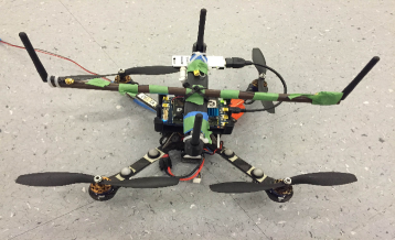
Figure 5: Chronos Personal Drone: We implement Chronos on an AscTec Hummingbird quadrotor with an AscTec Atomboard.

8 Computing Distances and Location

So far, we have explained how Chronos measures the time-of-flight between two antennas on a pair of Wi-Fi cards. One can then compute the distance between the two antennas (i.e., the two devices) by multiplying the time-of-flight by the speed of light. One can also compute the location by intersecting multiple such distances.

For example, consider a two-antenna receiver that aims to compute its location relative to a single-antenna transmitter. The receiver first applies Chronos’s algorithm to measure the time-of-flight of the transmitter’s signal to its two receive antennas. When multiplied by the speed of light this provides two distances of the two receive antennas from the transmitter. Hence, the transmitter must lie at the intersection of the two circles, centered around each receive antenna with radii defined by these distances.

In general, two distances are not enough to compute the location as two circles typically intersect at two points. Chronos can resolve the ambiguity using one of two strategies: (1) If the receiver has a third antenna, Chronos can use it to find a third circle on which the transmitter should lie. The three circles will together intersect at a unique point (assuming the antennas are not co-linear). Notice that if the three circles do not intersect exactly (e.g., due to noise), Chronos can use well-known least-squares optimizations to pick the point closest to the three circles [34]. Similarly, if the transmitter has more than one antenna, Chronos can improve the localization accuracy by computing pairwise distances between the transmit and receive antennas and then, incorporating them in the optimization problem. (2) A second approach to remove location ambiguity leverages mobility. A receiver can move towards what it believes to be the transmitter’s location, and re-run Chronos’s algorithm. If the transmitter indeed moved closer, the chosen location is correct. If not, one must pick the other possible location of the transmitter. We employ this strategy to disambiguate the transmitter’s location for the personal drone in §9.

9 Application to Personal Drones

To illustrate Chronos’s capabilities, we apply it to indoor personal drones [43]. These drones can follow users around while maintaining a convenient distance relative to the mobile device in the user’s pocket. Knowing the distance to the user allows the drone to take clear optimal pictures by ensuring that the user is within the frame of view at the right level of zoom. Users can leverage these drones to take pictures or videos of them while they are performing an activity, even in indoor settings where GPS is unavailable.

This application highlights Chronos’s unique benefits:

• Device-to-device solution: A key feature of Chronos is its ability to deliver device-to-device localization – i.e., enabling devices with commercial Wi-Fi cards to accurately localize each other without support from surrounding infrastructure. Thus, Chronos requires only a Wi-Fi enabled drone and a Wi-Fi device on the user. The user may use his personal drone to record his activities anywhere, whether at home, at work or in the gym, without requiring the access points in these buildings to support localization.

• Uses commercial Wi-Fi cards: Indoor drones can carry only limited payload for stable flight over long durations. In other words, drones simply cannot carry state-of-the-art accurate localization hardware such as antenna arrays. Fortunately, since Chronos is compatible with commodity Wi-Fi cards, it is possible integrate it with a light-weight computing module that weighs 90 grams and can be carried by small indoor drones.

We built Chronos over an AscTec Hummingbird quadrotor equipped with a Go-pro camera, as shown in Fig. 5. To localize the quadrotor, Chronos uses a 3-antenna Wi-Fi radio and intersects the distances of the user’s device to its 3-antennas. The distance measurements are integrated with drone navigation using a standard negative feedback-loop robotic controller [11]. Specifically, this controller measures the current distance of the user’s mobile device. If the user is closer than expected, the drone takes a discrete step further away and vice-versa. Such controllers are well-known to converge efficiently to stable solutions [11]. Our results in §12.4 show that Chronos converges to optimal locations that maintain stable distances. Further, our approach also benefits from an inherent synergy between Chronos’s localization and the robotic controller. Specifically, the feedback controller invokes Chronos’s algorithm multiple times to compute its precise distance to the user. In doing so, it can average across these invocations and reject outliers to maintain this distance at a much higher accuracy than Chronos’s native algorithm, as we show in §12.4.

10 Limitations and Trade-Offs

In this section, we discuss the limitations and trade-offs in Chronos’s design.

Frequency Band Hopping: Chronos requires wireless devices to hop between Wi-Fi frequency bands. Our implementation hops between all bands of Wi-Fi in 84 ms (see §12.3). A natural question to ask is how this hopping affects data traffic and user experience. Note that Chronos is primarily targeted for localization between a pair of Wi-Fi user devices that may otherwise not exchange data. However, some users may be interested in running Chronos on a single access point in home environments, where there may not be multiple access points covering the same physical space. Such access points cannot transmit/receive data to other clients as they localize. §12.3 shows that occasional demands for localization every tens of seconds minimally impacts TCP and video applications on these clients. But more frequent requests for localization may necessitate deploying a dedicated Chronos access point exclusively for in-home localization. Finally, since Chronos sends few packets per frequency band, it does not significantly impact nearby Wi-Fi networks.

Antenna Separation: Chronos’s accuracy in localizing a device improves with greater separation between its receive antennas. As the separation between a pair of antennas becomes larger, the resulting localization circles experience smaller overlap. This means that their point of intersection is less sensitive to noise, improving localization accuracy. Consequently, Chronos’s positioning accuracy on a Wi-Fi access point which can afford larger separation between antennas is higher than Chronos between a pair of user devices (e.g. laptops or tablets). Our results in §12.2 empirically evaluate this trade-off in typical indoor environments.

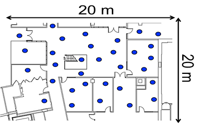
Figure 6: Testbed: Blue dots show candidate device locations.

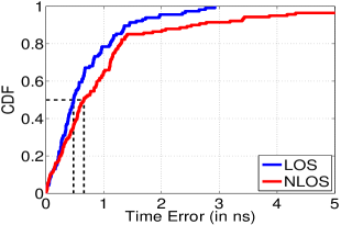
(a) Time of Flight

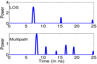
(b) Multipath Profiles

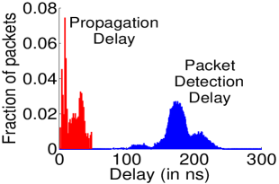
(c) Packet Detection Delay

Figure 7: Accuracy in Time of Flight: (a) measures the CDF of error in time-of-flight between two devices in Line of Sight (LOS) and Non-Line of Sight (NLOS). (b) plots representative multipath profiles. (c) plots histograms of time-of-flight and packet detection delay.

11 Implementation

We implemented Chronos as a software patch to the iwlwifi driver on Ubuntu Linux running the 3.5.7 kernel. To measure channel-state-information, we leverage the 802.11 CSI Tool [23] for the Intel 5300 Wi-Fi card. We measure wireless channels on both 2.4 GHz and 5 GHz Wi-Fi bands.

Unless specified otherwise, we pair two Chronos devices by placing each device in monitor mode with packet injection support on the same Wi-Fi frequency. We implemented Chronos’s channel hopping protocol (see §4) in the iwlwifi driver using high resolution timers (hrtimers), which can schedule kernel tasks such as packet transmits at microsecond granularity. Since the 802.11 CSI Tool does not report channel state information for Link-Layer ACKs received by the card, we use packet-injection to create and transmit special acknowledgments directly from the iwlwifi driver to minimize delay between packets and acknowledgments. These acknowledgments are also used to signal the next channel that the devices should hop to, as described in §4. Finally we process the channel state information to infer time-of-flight and device locations purely in software written in part in C++, MEX and MATLAB.

12 Results

We evaluate Chronos using the testbed in Fig. 6.

12.1 Accuracy in Time-of-Flight

In this experiment, we evaluate whether Chronos can deliver on its promise of measuring sub-nanosecond time-of-flight between a single pair of commodity Wi-Fi devices.

Method: We conduct our main experiments in a floor of a large office building measuring $20~{}\text{m}\times 20~{}\text{m}$ as shown in Fig. 6. The floor has multiple offices, a lounge area, conference rooms, metal cabinets, computers and furniture. We perform our experiments using two Thinkpad W300 Laptops equipped with 3-antenna Intel 5300 Wi-Fi cards. We placed the two devices randomly at any of 30 randomly chosen locations, as shown by the blue circles in the figure, with their pairwise distance up to $15$ m. We perform experiments for pairs of locations both in line-of-sight and non-line-of-sight. We measure the ground-truth of these locations using a combination of architectural drawings of our buildings and a Bosch GLM50 laser distance measurement tool [1], which measures distances up to 50 m with an accuracy of 1.5 mm. We repeat the experiment multiple times and measure the time-of-flight in each instance. We also compute the packet-detection delay of each packet using channel phase (see §5) to gauge its effect on the measurement of time-of-flight.

Time-of-Flight Results: We first evaluate Chronos’s accuracy in time-of-flight. Fig. 7(a) depicts the CDF of the time-of-flight of the signal in line-of-sight settings and non-line-of-sight. We observe that the median errors in time-of-flight estimation are 0.47 ns and 0.69 ns respectively (95${}^{\text{th}}$ percentile: 1.96 ns and 4.01 ns). Our results show that Chronos achieves its promise of computing time-of-flight at sub-nanosecond accuracy. To put this in perspective, consider SourceSync [45], a state-of-the-art system for time synchronization. SourceSync achieves 95${}^{\text{th}}$ percentile synchronization error up to 20 ns, using advanced software radios. In contrast, Chronos achieves order-of-magnitude lower error in time-of-flight using commodity Wi-Fi cards. However, we point out that unlike indoor positioning, tens of nanoseconds of error is sufficient for time-synchronization, which is the application SourceSync targets.

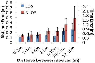
(a) Accuracy with distance

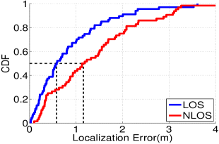
(b) Localization Error (Small separation)

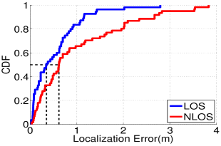
(c) Localization Error (Large separation)

Figure 8: (a) Accuracy with Distance: Plots the error in distance/time across the ground-truth distance between transmitter and receiver. (b, c) Localization Accuracy: Plots CDF of localization error using (b) a client with mean antenna separation of 30 cm and (c) an access point with antenna separation of 100 cm for transmitter and receiver in Line-of-Sight (LOS) and Non-Line-of-Sight (NLOS).

Multipath Profile Results: Next, we plot candidate multipath profiles computed by Chronos. Fig. 7(b) plots representative multipath profiles in line-of-sight and multipath environments. We note that both profiles are sparse, with the profile in multipath environments having five dominant peaks. Across experiments, the mean number of dominant peaks in the multipath profiles is 5.05 on average, with standard deviation 1.95 — indicating that they are indeed sparse. As expected, the profile in line-of-sight has even fewer dominant peaks than the profile in multipath settings. In both cases, we observe that the leftmost peaks in both the profiles correspond to the true location of the source. Further, we observe that the peaks in both profiles are sharp due to two reasons: 1) Chronos effectively spans a large bandwidth that includes all Wi-Fi frequency bands, leading to high time resolution; 2) Chronos’s resolution is further improved by exploiting sparsity that focuses on retrieving the sparse dominant peaks at much higher resolution, as opposed to all peaks.

Packet Detection Delay Results: We compare time-of-flight in indoor environments against packet detection delay. Fig. 7(c) depicts histograms of both packet detection delay and time-of-flight across experiments. Chronos observes a median packet detection delay of 177 ns across experiments. We emphasize two key observations: (1) Packet detection delay is nearly 8$\times$ larger than the time-of-flight in our typical indoor testbed. (2) It varies dramatically between packets, with a high standard deviation of 24.76 ns. In other words, packet detection delay is a large contributor to time-of-arrival that is highly variable, and therefore, hard to predict. This means that if left uncompensated, these delays could lead to a large error in time-of-flight measurements. Our results therefore reinforce the importance of accounting for these delays and demonstrate Chronos’s ability to do so.

Distance Results: Fig. 8(a) plots the median and standard deviation of error in distance computed between the transmitter and receiver against their true relative distance. We observe that this error is initially around 10 cm and increases to at most 25.6 cm at 12-15 meters. The increase is primarily due to reduced signal-to-noise ratio at further distances.

12.2 Localization Accuracy

Next, we evaluate Chronos’s accuracy in finding the indoor position of one device relative to another.

Method: We repeat the experiment for the setup in §12.1 using a pair of 3-antenna client laptops with antennas separated by a mean distance of 30 cm. We consider pairs of locations where the distance between the devices vary up to 15 m. We then measure the time-of-flight of the transmitter’s signal to each antenna of the receiver. We multiply this quantity by the speed of light to measure the pairwise distances between the antennas on the transmitter and the receiver. We perform outlier rejection on this set of distance estimates to discard estimates that do not fit the geometry of the relative antenna placements on these devices. Next, we use the remaining distance estimates to compute the location of the device using a least-square optimization formulation (as stated in §8). We repeat the experiment multiple times in line-of-sight and non-line-of-sight.

Results: Fig. 8(b) plots a CDF of localization error using Chronos in different settings. The device’s median positioning error for line of sight scenarios is 58 cm and 118 cm in line-of-sight and non-line-of-sight. Thus, Chronos achieves state-of-the-art indoor localization accuracy between a pair of user devices without third party support.

As mentioned in §10, Chronos’s accuracy depends on the separation between antennas. In particular, users may wish to run Chronos to localize their device relative to the single Wi-Fi access point in their home, where multiple access points covering the same area may be unavailable. Such an access point can afford greater separation between antennas than a user device. To evaluate this, we repeated the above experiment with the receiving laptop emulating a Wi-Fi access point with antennas separated by 100 cm. In this setting, the median localization error, reduces as expected to 35 cm and 62 cm in line-of-sight and non-line-of-sight (see Fig. 8(c)).

(a) Hopping Time

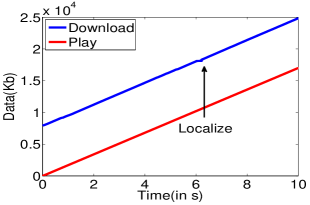
(b) Video Streaming

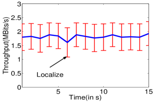
(c) TCP Throughput

Figure 9: Impact on Network Traffic: (a) measures the CDF time taken by Chronos to hop between all Wi-Fi bands – a small value of 84 ms. Consider a client-1 with a long-running traffic flow to an access point. The access point is asked to localize another client-2 at $t=6$ s. (b) depicts a representative trace of the number of bytes of data downloaded and data played over time if the client-1 views a VLC video stream. (c) measures the throughput if client-1 runs a TCP flow using iperf. In either case, the impact of client-1’s flow is minimal at $t=6$ s.

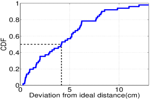
(a) Error in Distance

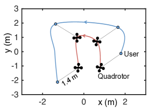
(b) Drone Trajectory

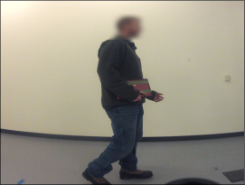
(c) Picture of User

Figure 10: Application to Personal Drones: The personal drone uses Chronos to maintain a constant distance of 1.4 m to the user. (a) depicts the CDF of error in distance of the drone relative to 1.4 m. (b) depicts a candidate trajectory of the drone. (c) shows an example picture of the user (face blurred for anonymity) taken by the drone. Since its Go-Pro uses a wide-angle lens, the user is fully in-frame at 1.4 m.

12.3 Impact on Network traffic

Chronos is primarily targeted to enable localization-between a pair of user devices, which may not otherwise communicate data between each other directly. However, an interesting question is the impact of Chronos on network traffic, if one of the devices is indeed serving traffic, e.g., a Wi-Fi access point. This experiment answers three questions in this regard: (1) How long does Chronos take to hop between all Wi-Fi bands? (2) How does Chronos impact real-time traffic like video streaming applications? (3) How does Chronos affect TCP? We address these questions below:

Method: We consider three Thinkpad W530 Laptops, one emulating an access point (using hostapd) and two clients. We assume client-2 requests the access point for indoor localization at $t=6~{}$s. We measure the time Chronos incurs to hop between the 35 Wi-Fi bands. Meanwhile, client-1 runs a long-lasting traffic flow. We consider two types of flows: (1) VLC video stream over RTP; (2) TCP flow using iperf. We repeat the experiment 30 times and find aggregate results.

Results: Fig. 9(a) depicts the CDF of the time that Chronos incurs to hop over all Wi-Fi bands. We observe that the median hopping time is 84 ms for the Intel 5300 Wi-Fi card, in tune with past work on other commercial Wi-Fi radios [31].

Next, Fig. 9(b) plots a representative trace of the cumulative bytes of video received over time of a VLC video stream run by client-1 (solid blue line). The red line plots the cumulative number of bytes of video played by the client. Notice that at $t=6~{}$s, there is a brief time span when no new bytes are downloaded by the client (owing to the localization request). However, in this interval, the buffer has enough bytes of video to play, ensuring that the user does not perceive a video stall (i.e. the blue and red lines do not cross). In other words, buffers in today’s video streaming applications can largely cushion such short-lived outages [28, 27], minimizing impact on user experience. Similarly, Fig. 9(c) depicts a representative trace of the throughput over time of a TCP flow at client-1. We observe that the TCP throughput dips only slightly by 6.5% at $t=6~{}$s, when client-2 requests location. However, we emphasize that if more frequent localization is desired, we recommend deploying an access point or Wi-Fi beacon exclusively for indoor positioning.

12.4 Application to Personal Drones

To illustrate Chronos’s capabilities, we evaluate how Chronos effectively guides a personal drone to follow a user’s device at an optimal distance to take pictures.

Method: Our personal drone is an AscTec Hummingbird quadrotor equipped with the AscTec Atomboard light-weight computing platform (with the Intel 5300 Wi-Fi card), a Go-pro camera and a Yei-Technology motion sensor. We 3-D print an enclosure to mount all these components safely atop the quadrotor. Fig. 5 depicts our setup. Note that the Intel 5300 Wi-Fi card supports 3-antennas; the fourth antenna on the quadrotor is placed only for balance and stability.

We perform our personal drone experiments in a $6~{}\text{m}\times 5~{}\text{m}$ room augmented with the VICON motion capture system [3]. The motion capture room uses an array of twelve infrared cameras to track devices tagged with infrared markers at sub-centimeter accuracy. We use the motion tracking system to find the ground-truth trajectories of the personal drone and user device. In each experiment, the personal drone tracks an ASUS EEPC netbook with the Intel 5300 Wi-Fi card held by a user. The user walks along a randomly chosen trajectory. The drone maintains a constant height and follows the user using Chronos’s negative-feedback loop algorithm, described in §9 to maintain a constant distance of 1.4 m relative to the user’s device. The drone also captures photographs of the user along the way using the Go-Pro camera mounted on the Hummingbird quadrotor, keeping the user at 1.4 m in focus. The drone uses the compass on the user’s device and the quadrotor to ensure that its camera always faces the user.

Results: Fig. 10(a) measures the CDF of root mean squared deviation in distance of the drone relative to the desired value of 1.4 m — a median of 4.17 cm. Our results reveal that the drone tightly maintains its relative distance to the user’s device. Notice that our error in distance is significantly lower in this experiment relative to §12.2. This is because drones measure multiple distances as they navigate in the air, which helps de-noise measurements and remove outliers (see §9).

Fig. 10(b) depicts a candidate overhead trajectory of the drone, captured using the Vicon motion capture system. The trajectory reveals that the drone follows the user’s location closely, as expected. Observe that at each point in its trajectory, the drone maintains a steady pairwise distance of 1.4 m relative to the device. Finally, Fig. 10(c) depicts a representative picture of the user that drone took along the way (face blurred for anonymity). Notice that the picture was taken at the optimal distance of 1.4 m and ensures that the user is at the right focus. Note that the Go-Pro uses a wide-angle lens which ensures that the user at 1.4 m is fully in-frame.

13 Conclusion

This paper presents Chronos, a system that measures sub-nanosecond time-of-flight on commercial Wi-Fi radios. Chronos leverages these time-of-flight measurements to demonstrate device-to-device indoor positioning at state-of-the-art accuracy, without third party support. To illustrate these capabilities, Chronos enables light-weight personal drones to track a user’s location in indoor environments. Beyond personal drones, Chronos opens up indoor positioning to many new contexts, where pairs of devices interact, e.g., gesture-based gaming consoles, finding lost devices, maintaining robotic formations, etc.

References

- [1] Bosch laser distance measurer glm50. http://www.boschtools.com/Products/Tools/Pages/BoschProductDetail.aspx?pid=GLM\%2050.
- [2] IEEE 802.11n-2009. http://standards.ieee.org/findstds/standard/802.11n-2009.html.
- [3] Vicon t-series. http://www.vicon.com/products/documents/Tseries.pdf.
- [4] F. Adib, Z. Kabelac, D. Katabi, and R. C. Miller. 3D Tracking via Body Radio Reflections. NSDI, 2014.
- [5] M. Angermann and P. Robertson. FootSLAM: Pedestrian Simultaneous Localization and Mapping Without Exteroceptive Sensors. Proceedings of the IEEE, 2012.
- [6] F. Bach, R. Jenatton, J. Mairal, and G. Obozinski. Convex optimization with sparsity-inducing norms, 2011.
- [7] S. Bagchi and S. K. Mitra. The Nonuniform Discrete Fourier Transform and Its Applications in Signal Processing. Kluwer Academic Publishers, Norwell, MA, USA, 1999.
- [8] P. Bahl and V. Padmanabhan. Radar: an in-building rf-based user location and tracking system. In INFOCOM, 2000.
- [9] W. U. Bajwa, J. Haupt, A. Sayeed, and R. Nowak. Compressed channel sensing: A new approach to estimating sparse multipath channels. In Proceedings of the IEEE, pages 1058–1076, 2010.
- [10] T. Bourchas, M. Bednarek, D. Giustiniano, and V. Lenders. Practical limits of wifi time-of-flight echo techniques. In IPSN, pages 273–274, April 2014.
- [11] Y. Brun, G. Marzo Serugendo, C. Gacek, H. Giese, H. Kienle, M. Litoiu, H. Müller, M. Pezzè, and M. Shaw. Software Engineering for Self-Adaptive Systems. chapter Engineering Self-Adaptive Systems Through Feedback Loops. 2009.
- [12] K. Chintalapudi, A. Padmanabha Iyer, and V. N. Padmanabhan. Indoor localization without the pain. MobiCom, 2010.
- [13] C. Ding, D. Pei, and A. Salomaa. Chinese Remainder Theorem: Applications in Computing, Coding, Cryptography. World Scientific Publishing Co., Inc., River Edge, NJ, USA, 1996.
- [14] A. Dutt and V. Rokhlin. Fast fourier transforms for nonequispaced data. SIAM J. Sci. Comput., 14(6):1368–1393, Nov. 1993.
- [15] J. Fang, K. Tan, Y. Zhang, S. Chen, L. Shi, J. Zhang, Y. Zhang, and Z. Tan. Fine-grained channel access in wireless lan. IEEE/ACM Trans. Netw., 21(3):772–787, June 2013.
- [16] B. Ferris et al. WiFi-SLAM using gaussian process latent variable models. IJCAI, 2007.
- [17] M. Fornasier. Numerical methods for sparse recovery. Theoretical Foundations and Numerical Methods for Sparse Recovery, 14:93–200, 2010.
- [18] S. Gezici, Z. Tian, G. B. Biannakis, H. Kobayashi, A. F. Molisch, V. Poor, Z. Sahinoglu, S. Gezici, Z. Tian, G. B. Giannakis, H. Kobayashi, A. F. Molisch, H. V. Poor, and Z. Sahinoglu. Localization via ultra-wideband radios. In IEEE Signal Processing Magazine, pages 70–84, 2005.
- [19] D. Giustiniano and S. Mangold. Caesar: Carrier sense-based ranging in off-the-shelf 802.11 wireless lan. CoNEXT, 2011.
- [20] J. Gjengset, J. Xiong, G. McPhillips, and K. Jamieson. Phaser: Enabling phased array signal processing on commodity wifi access points. MobiCom, 2014.
- [21] L. Greengard and J. yub Lee. Accelerating the nonuniform fast fourier transform. SIAM REVIEW, 46(3):443–454, 2004.
- [22] M. Guillaud, D. Slock, and R. Knopp. A practical method for wireless channel reciprocity exploitation through relative calibration. ISSPA, 2005.
- [23] D. Halperin, W. Hu, A. Sheth, and D. Wetherall. Tool release: Gathering 802.11n traces with channel state information. ACM SIGCOMM CCR, 2011.
- [24] M. Hazewinkel. Encyclopaedia of Mathematics: An Updated and Annotated Translation of the Soviet "Mathematical Encyclopaedia. Encyclopaedia of Mathematics. Springer Netherlands, 1997.
- [25] J. Heiskala and J. Terry, Ph.D. OFDM Wireless LANs: A Theoretical and Practical Guide. Sams, Indianapolis, IN, USA, 2001.
- [26] K. Hou, Z. Zhou, A. M.-C. So, and Z.-Q. Luo. On the linear convergence of the proximal gradient method for trace norm regularization. In Advances in Neural Information Processing Systems 26, pages 710–718. Curran Associates, Inc., 2013.
- [27] T.-Y. Huang, R. Johari, and N. McKeown. Downton Abbey Without the Hiccups: Buffer-based Rate Adaptation for HTTP Video Streaming. FhMN, 2013.
- [28] T.-Y. Huang, R. Johari, N. McKeown, M. Trunnell, and M. Watson. A Buffer-based Approach to Rate Adaptation: Evidence from a Large Video Streaming Service. SIGCOMM, 2014.
- [29] A. T. Islam and I. Misra. Performance of wireless ofdm system with ls-interpolation-based channel estimation in multi-path fading channel. IJCSA, 2012.
- [30] K. Joshi, S. Hong, and S. Katti. Pinpoint: Localizing interfering radios. NSDI, 2013.
- [31] S. Kandula, K. C.-J. Lin, T. Badirkhanli, and D. Katabi. FatVAP: Aggregating AP backhaul capacity to maximize throughput. In NSDI, 2008.
- [32] B. Kempke, P. Pannuto, and P. Dutta. Harmonia: Wideband Spreading for Accurate Indoor RF Localization. HotWireless, 2014.
- [33] M. Kohler, S. N. Patel, J. W. Summet, E. P. Stuntebeck, and G. D. Abowd. Tracksense: Infrastructure free precise indoor positioning using projected patterns. PERVASIVE, 2007.
- [34] S. Kumar, S. Gil, D. Katabi, and D. Rus. Accurate indoor localization with zero start-up cost. MobiCom, 2014.
- [35] S. Lanzisera, D. Zats, and K. Pister. Radio frequency time-of-flight distance measurement for low-cost wireless sensor localization. Sensors Journal, IEEE, 11(3):837–845, March 2011.
- [36] F. Li, C. Zhao, G. Ding, J. Gong, C. Liu, and F. Zhao. A Reliable and Accurate Indoor Localization Method Using Phone Inertial Sensors. UbiComp, 2012.
- [37] K. Liu et al. Guoguo: Enabling fine-grained indoor localization via smartphone. MobiSys, 2013.
- [38] A. Marcaletti, M. Rea, D. Giustiniano, V. Lenders, and A. Fakhreddine. Filtering noisy 802.11 time-of-flight ranging measurements. CoNEXT, 2014.
- [39] A. T. Mariakakis, S. Sen, J. Lee, and K.-H. Kim. Sail: Single access point-based indoor localization. MobiSys, 2014.
- [40] K. Muthukrishnan, G. Koprinkov, N. Meratnia, and M. Lijding. Using time-of-flight for wlan localization: feasibility study, 2006.
- [41] Y. Nakazato, M. Kanbara, and N. Yokoya. Localization system for large indoor environments using invisible markers. VRST, 2008.
- [42] A. Popleteev. Device-free indoor localization using ambient radio signals. UbiComp ’13 Adjunct, 2013.
- [43] B. Popper. The drone you should buy right now. http://www.theverge.com/2014/7/31/5954891/best-drone-you-can-buy.
- [44] Q. Pu, S. Gupta, S. Gollakota, and S. Patel. Whole-home gesture recognition using wireless signals. MobiCom, 2013.
- [45] H. Rahul, H. Hassanieh, and D. Katabi. SourceSync: A Distributed Wireless Architecture for Exploiting Sender Diversity. In ACM SIGCOMM 2010, New Delhi, India, August 2010.
- [46] H. Rahul, S. Kumar, and D. Katabi. MegaMIMO: Scaling Wireless Capacity with User Demands. In ACM SIGCOMM 2012, Helsinki, Finland, August 2012.
- [47] A. Rai, K. K. Chintalapudi, V. N. Padmanabhan, and R. Sen. Zee: zero-effort crowdsourcing for indoor localization. Mobicom ’12.
- [48] S. Ravindra and S. N. Jagadeesha. Time of arrival based localization in wireless sensor networks : A linear approach. CoRR, abs/1403.6697, 2014.
- [49] L. Schauer, F. Dorfmeister, and M. Maier. Potentials and limitations of wifi-positioning using time-of-flight. In IPIN, 2013.
- [50] S. Shin, C. Park, J. Kim, H. Hong, and J. Lee. Adaptive step length estimation algorithm using low-cost mems inertial sensors. In SAS, 2007.
- [51] A. Smith et al. Tracking Moving Devices with the Cricket Location System. In MobiSys, 2004.
- [52] D. Tse and P. Vishwanath. Fundamentals of Wireless Communications. Cambridge University Press, 2005.
- [53] F. Wen and C. Liang. An Indoor AOA Estimation Algorithm for IEEE 802.11ac Wi-Fi Signal Using Single Access Point. Communications Letters, IEEE, 2014.
- [54] F. Wen and C. liang. Fine-grained indoor localization using single access point with multiple antennas. Sensors Journal, IEEE, 2015.
- [55] S. B. Wibowo, M. Klepal, and D. Pesch. Time of flight ranging using off-the-self ieee802.11 wifi tags. POCA, 2009.
- [56] J. Xiong and K. Jamieson. Arraytrack: A fine-grained indoor location system. NSDI ’13, 2013.
- [57] J. Xiong, K. Jamieson, and K. Sundaresan. Synchronicity: Pushing the envelope of fine-grained localization with distributed mimo. HotWireless, 2014.
- [58] M. Youssef and A. Agrawala. The Horus WLAN location determination system. MobiSys, 2005.