Rare mutations limit of a steady state dispersal evolution model

Abstract

The evolution of a dispersal trait is a classical question in evolutionary ecology, which has been widely studied with several mathematical models. The main question is to define the fittest dispersal rate for a population in a bounded domain, and, more recently, for traveling waves in the full space.

In the present study, we reformulate the problem in the context of adaptive evolution. We consider a population structured by space and a genetic trait acting directly on the dispersal (diffusion) rate under the effect of rare mutations on the genetic trait. We show that, as in simpler models, in the limit of vanishing mutations, the population concentrates on a single trait associated to the lowest dispersal rate. We also explain how to compute the evolution speed towards this evolutionary stable distribution.

The mathematical interest stems from the asymptotic analysis which requires a completely different treatment for each variable. For the space variable, the ellipticity leads to the use the maximum principle and Sobolev-type regularity results. For the trait variable, the concentration to a Dirac mass requires a different treatment. This is based on the WKB method and viscosity solutions leading to an effective Hamiltonian (effective fitness of the population) and a constrained Hamilton-Jacobi equation.

Key words: Dispersal evolution; Nonlocal pde; Constrained Hamilton-Jacobi equation; Effective fitness;
Mathematics Subject Classification (2010): 35B25; 35F21; 92D15

1 Evolution of dispersion

Evolutionary dynamics of a structured population.

There are several well established mathematical formalisms to describe evolution. Game theory is widely used since the seminal paper [29]; see also [23]. Dynamical systems are also employed to describe the possible invasion of a population be a mutant, and to characterize Evolutionary Stable Strategies and other mathematical concepts; see, for instance, [16, 20]. Stochastic individual based models are often used to describe the evolution of individuals undergoing birth, death and mutations. Relations with other approaches can also been made at the large population limit, see [2, 12] and the references therein.

The formalism we use here is still different and relies on a population structured by a phenotypical trait and competing for a limited resource. This approach was initiated and has been widely studied in [17]. Several other versions use the formalism of a population structured by a trait, undergoing mutations and competition [34, 15, 25, 28]. All these papers, however, consider only proliferative advantage. The population with the highest birth rate or best competition ability survives while other traits undergo extinction. Mathematically this is represented by a limiting process where the population number density, denoted here by $n$, takes the form of a weighted Dirac concentrated at the fittest trait $\bar{\theta}$.

The extension to models, where the phenotypical trait is combined with another structuring variable, usually space, is more recent and leads to considerable mathematical difficulties; see [1, 9, 37, 30, 13, 10]. This is mainly due to the fact that for the trait variable $\theta$ the solutions concentrate as described above while in the space variable solutions remain bounded.

Another motivation for considering the model in this note is to study the selection of the fittest individuals without a proliferative advantage. In this context, the reproduction rate might be compensated by another advantage. This gives rise to the question of defining an “effective fitness.” The gradient of the effective fitness determines the direction of trait evolution and its maximum defines the evolutionary stable strategy.

A particularly interesting example, both mathematically and biologically, in this directions is the selection of a dispersal rate, which we describe next in the context of a continuous dispersal trait. When only two species are represented by their number densities $n_{1}(x)$, $n_{2}(x)$ and are competing for the same resource (carrying capacity) $K$, the question is to know which of the two dispersal rates $D_{1}$, $D_{2}$ is prefered in the competiton. Then, the model is

$$-D_{i}\Delta_{x}n_{i}=n_{i}\big{(}K(x)-n_{1}+n_{2}\big{)},\qquad x\in\Omega,\quad i=1,\;2.$$

Is it better to ‘move’ faster or slower? In other words, is it favorable to have $D_{1}>D_{2}$ or the contrary?

The model.

Here we assume that all dispersal rates are possible, and include mutations. We ask the question of the rare mutation limit of the steady state version for a still simple model of evolution of dispersal in a population. The main modeling assumptions are: (i) all individuals wear a phenotype characterized by a parameter $\theta$, which induces a dispersal rate $D(\theta)$, (ii)  a Fisher-type Lotka-Volterra growth/death rate with a space dependent carrying capacity $K$ and limitation by the total population whatever the trait is, and (iii) rare mutations acting on the genetic variable and modeled by a diffusion with covariance $\sqrt{2}\varepsilon$; we refer to [12] for a derivation of this type of equations from individual based stochastic models.

More precisely, we study the asymptotic behavior, as $\varepsilon\to 0$, of the density $n_{\varepsilon}=n_{\varepsilon}(x,\theta):\Omega\times\mathbb{R}\to(0,\infty)$, with $\Omega\subset\mathbb{R}^{d}$ a smooth domain, of the nonlocal and nonlinear problem

$$\begin{cases}-D(\theta)\Delta_{x}n_{\varepsilon}-\varepsilon^{2}\Delta_{\theta}n_{\varepsilon}=n_{\varepsilon}\big{(}K(x)-\rho_{\varepsilon}(x)\big{)}\ \ \text{in }\ \ \Omega\times\mathbb{R},\\[1.0pt] \rho_{\varepsilon}(x)=\displaystyle\int_{0}^{1}n_{\varepsilon}(x,\theta)d\theta,\end{cases}$$ (1)

with Neumann boundary condition on $\partial\Omega$ and $1-$ periodicity in $\theta$, that is, if $\nu$ is the external normal vector to $\Omega$,

$$\frac{\partial}{\partial\nu}n_{\varepsilon}=0\ \text{ on}\ \partial\Omega\times\mathbb{R}\ \text{and}\ n_{\varepsilon}\ \text{is }\ 1-\text{periodic in}\ \theta.$$ (2)

We have chosen periodic boundary conditions in $\theta$ to simplify some technical aspects concerning a priori estimates.

As far as the carrying capacity $K$ and the dispersion rate $D$ are concerned, we assume

$$K\in C^{1}(\bar{\Omega}),\qquad\text{there exists $K_{m}>0$ such that}\ K(x)\geq K_{m}>0,\qquad K\text{ is not constant}.$$ (3)

and

$$\left\{\begin{array}[]{l}D\in C^{1}\big{(}\mathbb{R};(0,\infty)\big{)}\ \text{ is}\ 1\text{-periodic and}\\[2.84526pt] \text{ there exists a unique local minimizer $\theta_{m}\in[0,1)$ such that}\ D\geq D(\theta_{m}):=D_{m}>0;\end{array}\right.$$ (4)

we note (4) is used to assert that the effective Hamiltonian also has a minimum at $\theta_{m}$.

Finally, for technical reasons, we also assume that

$$\Omega\ \text{is convex}.$$ (5)

It follows from, for example, [3, 14], that, given (3) and (4), the problem (1) and (2) admits a strictly positive solution $n_{\varepsilon}:\Omega\times\mathbb{R}\to(0,\infty)$.

Formal derivation of the mathematical result.

We proceed now formally to explain what happens in the limit $\varepsilon\to 0$ and, hence, motivate the statement of the results. As it is often the case with problems where it is expected to see concentration in the limit, we make the exponential change of variables

$$n_{\varepsilon}=\exp\big{(}{u_{\varepsilon}}/{\varepsilon}\big{)},$$ (6)

which leads to

$$-\frac{D(\theta)}{\varepsilon}\Delta_{x}u_{\varepsilon}-\frac{D(\theta)}{\varepsilon^{2}}|\nabla_{x}u_{\varepsilon}|^{2}-\varepsilon\Delta_{\theta}u_{\varepsilon}-|\nabla_{\theta}u_{\varepsilon}|^{2}=K(x)-\rho_{\varepsilon}(x)\ \text{ in }\ \Omega\times\mathbb{R},$$ (7)

with

$$u_{\varepsilon}\ \text{is $1-$periodic in $\theta$}\ \text{ and }\ \frac{\partial}{\partial\nu}u_{\varepsilon}=0\ \text{ on}\ \partial\Omega\times\mathbb{R}.$$ (8)

It is clear from (7) that, if the $u_{\varepsilon}$’s have, as $\varepsilon\to 0$, a limit $u$, it must be independent of $x$, and, hence, it is natural to expect the expansion

$$u_{\varepsilon}(x,\theta)=u(\theta)+\varepsilon\ln{\mathcal{N}}(x,\theta)+O(\varepsilon).$$ (9)

Assuming that, as $\varepsilon\to 0$, the $\rho_{\varepsilon}$’s converge to some $\rho$, a formal computation suggests that ${\mathcal{N}}$ is the positive eigenfunction of

$$\begin{cases}-D(\theta)\Delta_{x}{\mathcal{N}}={\mathcal{N}}\;\big{(}K-\rho\big{)}+{\mathcal{N}}\;H\big{(}\theta,\rho(\cdot)\big{)}\ \text{in}\ \Omega,\\[2.84526pt] \frac{\partial}{\partial\nu}{\mathcal{N}}=0\ \text{on }\partial\Omega,\end{cases}$$ (10)

with eigenvalue $H\big{(}\theta,\rho(\cdot)\big{)}$, and that $u$ solves the constrained Hamilton-Jacobi equation

$$\begin{cases}-|\nabla_{\theta}u|^{2}=-H\big{(}\theta,\rho(\cdot)\big{)}\ \text{ in }\ \mathbb{R},\\[2.84526pt] \max_{\theta\in\mathbb{R}}u(\theta)=0,\\[2.84526pt] u\ \text{is $1-$ periodic}.\end{cases}$$ (11)

The constraint on the $\max u$ becomes evident from the facts that, as it turns out, the $\rho_{\varepsilon}$’s are bounded uniformly in $\varepsilon$ and the equality

$$\rho_{\varepsilon}(x)=\int_{0}^{1}n_{\varepsilon}(x,\theta)d\theta=\int_{0}^{1}\exp\big{(}u_{\varepsilon}(x,\theta)/\varepsilon\big{)}d\theta,$$ (12)

which also suggests that, as $\varepsilon\to 0$, the $n_{\varepsilon}$’s behave like a Dirac mass with weight $\rho$.

The mathematical result.

To state the result we recall that $\delta$ denotes the Dirac mass at $0$ and we introduce the nonlinear Fisher-type stationary problem

$$\begin{cases}-D_{m}\Delta_{x}N_{m}=N_{m}\;(K-N_{m})\ \text{on}\ \Omega\\[2.84526pt] \frac{\partial}{\partial\nu}N_{m}=0\ \text{ on}\ \partial\Omega,\end{cases}$$ (13)

which, in view of (3) and (4), admits a positive solution $N_{m}>0$ (see, for example, [3, 14].)

We have:

Theorem 1.1

Assume (3), (4), and (5). Then, as $\varepsilon\to 0$ and in the sense of distributions,

$$n_{\varepsilon}\to N_{m}(x)\delta(\theta-\theta_{m})\quad\text{ and}\quad\rho_{\varepsilon}\to N_{m}.$$

Moreover, as $\varepsilon\to 0$ and uniformly in $x$ and $\theta$, $\varepsilon\ln n_{\varepsilon}\to u$, where $u$ is the unique $1-$periodic solution to (11), with $\rho=N_{m}$, such that $\max u=u(\theta_{m})=0.$

Biological interpretation.

The conclusions of Theorem 1.1 can be thought as a justification of the fact that the population selects the “slowest” individuals in accordance with several previous observations on the evolution of dispersal. In this respect, the eigenvalue $-H\big{(}\theta,\rho(\cdot)\big{)}$ defines the fitness of individuals depending upon their trait. This fact can be stated using the canonical equation (31), which is formally derived in Section 6. In the words of adaptive dynamics, our result characterizes the unique Evolutionary Stable Distribution (or Strategy), [16, 25].

That mutants with lower dispersal rates can invade a population, that is the characterization of $\theta_{m}$ by property (4), is known from the first mathematical studies [22, 18]. However, these papers use time scale separation, heuristically assuming a mutant appears, with ‘small mutation’, and compete with the resident population. Our approach here is more intrinsic since we consider structured populations competing for resources and undergoing mutations. Surprisingly when set in the full space where the problem is characterized in terms of traveling waves, the opposite effect is observed, that is mutants with higher dispersal rates are selected giving rise to accelerating waves, [8, 9, 37, 4, 5]. For two competing populations, the combined effect of dispersal and a drift is studied in [21]. The analysis of dispersal evolution also gave rise to the notion of ideal free distribution [11, 13].

The question of dispersal evolution is a classical and important topic in evolutionary biology. The reader can consult [36] for a survey of the many related issues, to [33] for the case with patches and demographic stochasticity, to [24] for the case of trajectories with jumps (nonlocal operators) and to [8] for other biological references about accelerating fronts. A formalism using Fokker-Planck equation is used in [35]. Also, let us mention that a remarkable qualitative aspect fo spatial sorting is that in the full space, the largest dispersion rate is selected [8, 6, 7]. Finally, another mathematical approach to the concentration effect, stated in Theorem 1.1, can be found in [26].

Organization of the paper.

In Section 2 we prove some uniform in $\varepsilon$ estimates for the $\rho_{\varepsilon}$’s that are then used in Section  3 where we derive the effective Hamiltonian, that is the eigenvalue problem of (10). In Section  4 we introduce the constrained Hamilton-Jacobi equation to conclude the proof of Theorem 1.1 and Theorem 21. In Section  5 we prove the two technical lemmata that were used in Section  4. Finally, In Section  6, we provide some perspectives about the problem, namely a more precise asymptotic expansion and the parabolic case, as well as numerical examples for the evolution driven by the parabolic equation.

2 Estimates on $\rho_{\varepsilon}$

We state and prove here some, uniform in $\varepsilon$, estimates for the $\rho_{\varepsilon}$’s, which are fundamental for the analysis in the rest of the paper; here $|\Omega|$ is the measure of $\Omega$ and $C(A)$ denotes a constant that depends on $A$.

Lemma 2.1

Assume (3) and (4). There exist positive independent of $\varepsilon$ constants $C_{1}=C_{1}(K,D,\Omega)$, $C_{2}=C_{2}(K,D,\Omega)$ and $C_{3}=C_{3}(|\Omega|,\min K)$ such that

$$\begin{cases}(i)~{}\ \ 0\leq\rho_{\varepsilon}\leq C_{1},\\[2.84526pt] (ii)~{}\ \sup_{\varepsilon\in(0,1)}\|\rho_{\varepsilon}\|_{W^{2,p}(\Omega)}\leq C_{2}\ \text{ for all $p\in[1,\infty)$, and}\\[2.84526pt] (iii)~{}\int_{\Omega}\rho_{\varepsilon}(x)dx\geq C_{3},\end{cases}$$ (14)

and, along subsequences $\varepsilon\to 0$, the $\rho_{\varepsilon}$’s converge uniformly in $\overline{\Omega}$ to $\rho\in C(\overline{\Omega}).$

Proof. We first observe that $\rho_{\varepsilon}$ trivially satisfies the Neumann condition

$$\frac{\partial}{\partial\nu}\rho_{\varepsilon}=0\ \text{ on}\ \partial\Omega.$$ (15)

After dividing (1) by $D(\theta)$, integrating in $\theta$ and using the periodicity in $\theta$, we find

$$-\Delta_{x}\rho_{\varepsilon}-\varepsilon^{2}\int_{0}^{1}n_{\varepsilon}(x,\theta)\Delta_{\theta}\frac{1}{D}d\theta=\int_{0}^{1}\frac{1}{D}n_{\varepsilon}d\theta\;(K-\rho_{\varepsilon}),$$

and, hence, for some constant $C$, which only depends on $D$ and $K$, we have

$$-\Delta_{x}\rho_{\varepsilon}+\frac{1}{\|D\|_{\infty}}\rho_{\varepsilon}^{2}\leq C\rho_{\varepsilon}.$$

Then (14)(i) follows from the strong maximum principle, while the $W^{2,p}$-estimates are a consequence of the classical elliptic regularity theory.

The lower bound (14)(iii) comes from integrating (1) in $x$ and $\theta$. Indeed, in view of the assumed periodicity, we find

$$\max K\int_{\Omega}\rho_{\varepsilon}(x)dx\geq\int_{\Omega}\rho_{\varepsilon}(x)K(x)dx=\int_{\Omega}\rho_{\varepsilon}(x)^{2}dx\geq\frac{1}{|\Omega|}\left(\int_{\Omega}\rho_{\varepsilon}(x)dx\right)^{2}.$$

The last claim is an immediate consequence of the a priori estimates and the usual Sobolev imbedding theorems.

      

3 The effective Hamiltonian

For $\theta\in[0,1]$ and $\rho\in L^{\infty}\big{(}\Omega;[0,\infty)\big{)}$ we consider the eigenfunction ${\mathcal{N}}={\mathcal{N}}\big{(}\cdot;\theta,\rho(\cdot)\big{)}\in H^{1}(\Omega)$ and the eigenvalue $H=H\big{(}\theta,\rho(\cdot)\big{)}$ of

$$\begin{cases}-D(\theta)\Delta_{x}{\mathcal{N}}={\mathcal{N}}\;(K-\rho)+{\mathcal{N}}\;H\quad\text{in}\ \Omega,\\[2.84526pt] \frac{\partial}{\partial\nu}{\mathcal{N}}=0\ \text{on }\partial\Omega\qquad\text{and}\ \ \int_{\Omega}{\mathcal{N}}\big{(}x;\theta,\rho(\cdot)\big{)}^{2}dx=1.\end{cases}$$ (16)

Note that in view of (3) and the regularity of $\Omega$, the existence of the pair $\big{(}{\mathcal{N}}\big{(}\cdot;\theta,\rho(\cdot)\big{)},H\big{(}\theta,\rho(\cdot)\big{)}\big{)}$ follows from, for example, [3, 14].

The next lemma provides some important estimates and information about $H\big{(}\theta,\rho(\cdot)\big{)}$. In the statement we use the notation $K_{M}:=\max_{\overline{\Omega}}K.$

Lemma 3.1

Assume (3) and (4). Then

$$(i)\ -K_{M}\leq H\big{(}\theta,\rho(\cdot)\big{)}\ \ \text{and}\ \ (ii)\ H\big{(}\theta,\rho(\cdot)\big{)}\leq\frac{1}{|\Omega|}\int_{\Omega}\rho(x)dx,$$ (17)

$$\text{ the maps $\theta\to H\big{(}\theta,\rho(\cdot)\big{)}$ and $\theta\to D(\theta)$ have the same monotonicity properties for all $\rho$},$$ (18)

and, in particular, $\theta_{m}$ is the unique minimum of $H(\theta,\rho)$ in $[0,1]$ for all $\rho$.

Proof. Multiplying the equation by ${\mathcal{N}}$ and integrating in $x$ gives

$$0\leq D(\theta)\int_{\Omega}|\nabla{\mathcal{N}}|^{2}=\int_{\Omega}{\mathcal{N}}^{2}[K-\rho+H]dx\leq\int_{\Omega}{\mathcal{N}}^{2}dx\;[K_{M}+H],$$

and, thus, (17)(i) holds.

The upper bound (17)(ii) follows from the positivity of $K$, since, after dividing the equation by ${\mathcal{N}}$ and integrating by parts, we find

$$-\int_{\Omega}\frac{\big{|}\nabla_{x}{\mathcal{N}}\big{|}^{2}}{{\mathcal{N}}^{2}}dx=\int_{\Omega}[K-\rho+H]\,dx\leq 0.$$

For (18), we differentiate in $\theta$ the equation in (16) to find

$$-D^{\prime}(\theta)\Delta_{x}{\mathcal{N}}-D(\theta)\Delta_{x}{\mathcal{N}}_{\theta}={\mathcal{N}}_{\theta}\;\big{(}K(x)-\rho(x)+H\big{)}+{\mathcal{N}}\;H_{\theta},$$ (19)

where ${\mathcal{N}}_{\theta}$ and $H_{\theta}$ denote derivatives with respect to $\theta$, we multiply by ${\mathcal{N}}$ and integrate by parts using the boundary condition to get

$$D^{\prime}(\theta)\int_{\Omega}\big{|}\nabla_{x}{\mathcal{N}}\big{|}^{2}+D(\theta)\int\nabla_{x}{\mathcal{N}}.\nabla_{x}{\mathcal{N}}_{\theta}=\int{\mathcal{N}}{\mathcal{N}}_{\theta}[K-\rho]+H_{\theta}\big{(}\theta;\rho(\cdot)\big{)}.$$ (20)

Next we use the fact that the $L^{2}-$normalization of ${\mathcal{N}}$ yields $\int_{\Omega}{\mathcal{N}}_{\theta}{\mathcal{N}}dx=0$ and after multiplying the equation in (16) by ${\mathcal{N}}_{\theta}$, integrating by parts and subtracting the result from (20) we find

$$D^{\prime}(\theta)\int_{\Omega}\big{|}\nabla_{x}{\mathcal{N}}\big{|}^{2}=H_{\theta}\big{(}\theta;\rho(\cdot)\big{)}.$$

Since we have assumed in (3) that $K$ is not constant, $\nabla_{x}{\mathcal{N}}$ does not vanish and the result follows.

To conclude, we observe that (4) and (18) yield that $H$ as the same monotonicity, in $\theta$, as $D$ and, thus, has a unique local minimum at $\theta_{m}$.

      

4 The constrained Hamilton-Jacobi equation

We prove here the generalized Gaussian-type convergence asserted in Theorem 1.1, derive the constrained Hamilton-Jacobi equation (11) and state some more properties. For the benefit of the reader we restate these assertions as a separate theorem below.

Theorem 4.1

The family $u_{\varepsilon}$ is uniformly in $\varepsilon$ Lipschitz continuous and converges, uniformly in $x$ and $\theta$, to $u$, which is independent of $x$ and satisfies, in the viscosity sense, the constrained Hamilton-Jacobi equation (11). Moreover,

$$\min_{\theta}H\big{(}\theta,\rho(\cdot)\big{)}=0=H\big{(}\theta_{m},\rho(\cdot)\big{)}=H_{\theta}\big{(}\theta_{m},\rho(\cdot)\big{)}.$$ (21)

Since $-H$ represents the fitness, it turns out that (21) characterizes $\delta(\theta-\theta_{m})$ as the Evolutionary Stable Distribution (or $\theta_{m}$ as the Evolutionary Stable Strategy). See [16, 25].

It follows from (21) that both $H$ and its derivative vanish at $\theta_{m}$. As a result the viscosity solution $u$ of (11) also vanishes at $\theta_{m}$ as $u(\theta)=O\big{(}(\theta-\theta_{m})^{3/2}\big{)}$, and this makes the connection with the result of [26].

The proof is a consequence of the next two lemmata which are proved later in the paper.

Lemma 4.2 (Bounds on $u_{\varepsilon}$)

There exists an independent of $\varepsilon$ constant $C$ such that

$$\int_{\Omega}\max_{\theta}u_{\varepsilon}(x,\theta)dx\leq C\varepsilon.$$ (22)

Lemma 4.3 (Lipschitz estimates)

There exist an independent of $\varepsilon$ constant $C$ such that

$$\frac{1}{\varepsilon^{2}}|\nabla_{x}u_{\varepsilon}|^{2}+|\nabla_{\theta}u_{\varepsilon}|^{2}\leq C\quad\text{and}\quad\max_{x\in\Omega,0\leq\theta\leq 1}u_{\varepsilon}(x,\theta)\leq C\varepsilon.$$

Moreover, the $u_{\varepsilon}$’s converge, along a subsequence $\varepsilon\to 0$ and uniformly in $x$ and $\theta$, to a Lipschitz and $1$-periodic function $u:\mathbb{R}\to\mathbb{R}$ such that $\max_{0\leq\theta\leq 1}u(\theta)=0.$

We continue with the proofs of Theorem 21 and Theorem 1.1.

Proof of Theorem 21. The fact that any limit $u$ of the $u_{\varepsilon}$’s satisfies (11) is a standard application of the so-called perturbed test function method (see [19]) and we do not repeat the argument.

It follows from (11) that $H\big{(}\theta,\rho(\cdot)\big{)}\geq 0$, while, at any maximum point $\bar{\theta}$ of $u$, we must have $H\big{(}\bar{\theta},\rho(\cdot)\big{)}\leq 0$, and, hence, $H\big{(}\bar{\theta},\rho(\cdot)\big{)}=0,$ and, in view of Lemma 3.1,

$$\min_{\theta}H\big{(}\theta,\rho(\cdot)\big{)}=0=H\big{(}\theta_{m},\rho(\cdot)\big{)}.$$

As a result the only possible maximum point of any solution of (11) must be at at $\theta_{m}$, which implies that the equation has a unique solution.

Also the knowledge of $\theta_{m}$ determines uniquely the limit $\rho(x)=N_{m}(x)$, from equation (13), and, thus, the full family $(\rho_{\varepsilon},u_{\varepsilon})$ converges.

      

Proof of Theorem 1.1. The statement in terms of $n_{\varepsilon}$ is an immediate consequence of Theorem 21. Because $u_{\varepsilon}$ achieves a unique maximum at $\theta_{m}$, from the Laplace formula for $n_{\varepsilon}$ written as (6), we conclude that the $n_{\varepsilon}(x,\theta)$’s converge weakly in the sense of measures to $\rho(x)\delta(\theta-\theta_{m})$, with $\rho(x)$ the limit of $\rho_{\varepsilon}$ (see Section 2).

Next, integrating equation (1) in $\theta$ we conclude that

$$-\Delta\int_{0}^{1}D(\theta)n_{\varepsilon}d\theta=\rho_{\varepsilon}(x)\big{(}K(x)-\rho_{\varepsilon}(x)\big{)}.$$

Passing to the limit $\varepsilon\to 0$, and taking into account that $n$ is a Dirac mass at $\theta_{m}$, we find that $\rho=N_{m}$ because they both satisfy the equation (13).

      

5 The proofs

We begin with the proof of Lemma 22

Proof of Lemma 22. Integrating (7), we find

$$\frac{1}{\varepsilon^{2}}\int\int|\nabla_{x}u_{\varepsilon}|^{2}dxd\theta+\int\int|\nabla_{\theta}u_{\varepsilon}|^{2}dxd\theta\leq C.$$ (23)

The claim for the maximum bound follows from the $L^{\infty}-$estimate on $\rho_{\varepsilon}$.

For each $x\in\Omega$, let $M_{\varepsilon}(x):=\max_{\theta}u_{\varepsilon}(x,\theta)$ and choose $\theta_{\varepsilon}(x)$ such that $M_{\varepsilon}(x)=u_{\varepsilon}(x,\theta_{\varepsilon}(x)).$ Then it follows from (14)(i) that

$$e^{M_{\varepsilon}(x)/\varepsilon}\int_{0}^{1}e^{\big{(}u_{\varepsilon}(x,\theta)-u_{\varepsilon}(x,\theta_{\varepsilon})\big{)}/\varepsilon}d\theta=\rho_{\varepsilon}(x)\leq C.$$ (24)

Inserting in (24) the estimate

$$u_{\varepsilon}(x,\theta)-u_{\varepsilon}(x,\theta_{\varepsilon}(x))=\int_{\theta}^{\theta_{\varepsilon}(x)}\partial_{\theta}u_{\varepsilon}(x,\theta^{\prime})d\theta^{\prime}\geq-1-\int_{0}^{1}|\partial_{\theta}u_{\varepsilon}(x,\theta^{\prime})|^{2}d\theta^{\prime},$$

we get

$$e^{M_{\varepsilon}(x)/\varepsilon}\;e^{\displaystyle-\frac{1}{\varepsilon}[1+\int_{0}^{1}|\partial_{\theta}u_{\varepsilon}(x,\theta^{\prime})|^{2}d\theta^{\prime}]}\leq C,$$

and, hence,

$$\frac{M_{\varepsilon}(x)}{\varepsilon}-\frac{1}{\varepsilon}[1+\int_{0}^{1}|\partial_{\theta}u_{\varepsilon}(x,\theta^{\prime})|^{2}d\theta^{\prime}]\leq\ln C.$$

Using (23), we obtain

$$\int_{\Omega}M_{\varepsilon}(x)dx\leq C\varepsilon,$$

and this concludes the proof.

      

Next we discuss the proof of Lemma 4.3.

Proof of Lemma 4.3. We first assume the Lipschitz bound and prove the rest of the claims.

Let ${\mathcal{M}_{\varepsilon}}:=\max_{x\in\overline{\Omega}}M_{\varepsilon}(x)$, with $M_{\varepsilon}(x)$ as in the proof of the previous lemma. It is immediate from (22) and the fact that $|\nabla_{x}u_{\varepsilon}|^{2}\leq\varepsilon C$ that, for some $C>0$,

$${\mathcal{M}_{\varepsilon}}\leq\varepsilon C.$$

Next we show that $\liminf_{\varepsilon\to 0}{\mathcal{M}_{\varepsilon}}\geq 0$, which, in turn, yields that $\lim_{\varepsilon\to 0}{\mathcal{M}_{\varepsilon}}=0$.

Let $y_{\varepsilon}\in\overline{\Omega}$ be such that ${\mathcal{M}_{\varepsilon}}:=M_{\varepsilon}(y_{\varepsilon})=u_{\varepsilon}\big{(}y_{\varepsilon},\theta_{\varepsilon}(y_{\varepsilon})\big{)}$ and write

$$\rho_{\varepsilon}(x)=e^{\mathcal{M}_{\varepsilon}/\varepsilon}\int_{0}^{1}e^{\big{(}u_{\varepsilon}(x,\theta)-u_{\varepsilon}(y_{\varepsilon},\theta_{\varepsilon})\big{)}/\varepsilon}d\theta.$$

Combining the lower bound on $\rho_{\varepsilon}$ in Lemma 2.1 and the (Lipschitz) estimate $|\nabla_{x}u_{\varepsilon}|^{2}\leq\varepsilon C$, we get

$$C_{3}\leq\int_{\Omega}\rho_{\varepsilon}(x))\leq|\Omega|e^{\mathcal{M}_{\varepsilon}/\varepsilon}e^{C}\int_{0}^{1}e^{\big{(}u_{\varepsilon}(y_{\varepsilon},\theta)-u_{\varepsilon}(y_{\varepsilon},\theta_{\varepsilon})\big{)}/\varepsilon}d\theta\leq e^{\mathcal{M}_{\varepsilon}/\varepsilon}e^{C}|\Omega|,$$

and, thus, $\mathcal{M}_{\varepsilon}\geq-C\varepsilon$.

Now we turn to the proof of the Lipschitz bounds, which is an appropriate modification of the classical Bernstein estimates to take into account the different scales. We note and prove Lemma 4.3. Note that the convexity assumption on $\Omega$ is used solely in this proof.

We begin by writing the equations satisfied by $|D_{x}u_{\varepsilon}|^{2}$ and $|\partial_{\theta}u_{\varepsilon}|^{2}$ which we obtain by differentiating (7) in $x$ and $\theta$ and multiplying by $D_{x}u_{\varepsilon}$ and $\partial_{\theta}u_{\varepsilon}$. We have:

$$\begin{array}[]{rl}-\frac{D(\theta)}{\varepsilon}\Delta_{x}|D_{x}u_{\varepsilon}|^{2}-&\varepsilon\Delta_{\theta}|D_{x}u_{\varepsilon}|^{2}+2\frac{D(\theta)}{\varepsilon}|D^{2}_{xx}u_{\varepsilon}|^{2}+2\varepsilon|D^{2}_{x\theta}u_{\varepsilon}|^{2}\\[15.0pt] &-2\frac{D(\theta)}{\varepsilon^{2}}D_{x}u_{\varepsilon}.D_{x}|D_{x}u_{\varepsilon}|^{2}-2\partial_{\theta}u_{\varepsilon}.\partial_{\theta}|D_{x}u_{\varepsilon}|^{2}=2D_{x}(K-\rho_{\varepsilon}).Du_{\varepsilon},\end{array}$$ (25)

and

$$\begin{array}[]{rl}-\frac{D(\theta)}{\varepsilon}&\Delta_{x}|\partial_{\theta}u_{\varepsilon}|^{2}-\varepsilon\Delta_{\theta}|\partial_{\theta}u_{\varepsilon}|^{2}+2\frac{D(\theta)}{\varepsilon}|D^{2}_{x\theta}u_{\varepsilon}|^{2}+2\varepsilon|D^{2}_{\theta\theta}u_{\varepsilon}|^{2}\\[15.0pt] &-2\frac{D(\theta)}{\varepsilon^{2}}D_{x}u_{\varepsilon}.D_{x}|\partial_{\theta}u_{\varepsilon}|^{2}-2\partial_{\theta}u_{\varepsilon}.\partial_{\theta}|\partial_{\theta}u_{\varepsilon}|^{2}=2\frac{D^{\prime}(\theta)}{\varepsilon}\Delta_{x}u_{\varepsilon}\partial_{\theta}u_{\varepsilon}+4\frac{D^{\prime}(\theta)}{\varepsilon^{2}}|D_{x}u_{\varepsilon}|^{2}\partial_{\theta}u_{\varepsilon}.\end{array}$$ (26)

Let $q=\frac{|D_{x}u_{\varepsilon}|^{2}}{\varepsilon^{2}}+|\partial_{\theta}u_{\varepsilon}|^{2}$ and compute

$$\begin{array}[]{rl}-&\frac{D(\theta)}{\varepsilon}\Delta_{x}q-\varepsilon\Delta_{\theta}q+2\frac{D(\theta)}{\varepsilon^{3}}|D^{2}_{xx}u_{\varepsilon}|^{2}+\frac{1+D(\theta)}{\varepsilon}|D^{2}_{x\theta}u_{\varepsilon}|^{2}+2\varepsilon|D^{2}_{\theta\theta}u_{\varepsilon}|^{2}\\[15.0pt] &-2\frac{D(\theta)}{\varepsilon^{2}}D_{x}u_{\varepsilon}.D_{x}q-2\partial_{\theta}u_{\varepsilon}.\partial_{\theta}q=\frac{2}{\varepsilon^{2}}D_{x}(K-\rho_{\varepsilon}).Du_{\varepsilon}+2\frac{D^{\prime}(\theta)}{\varepsilon}\Delta_{x}u_{\varepsilon}\partial_{\theta}u_{\varepsilon}+4\frac{D^{\prime}(\theta)}{\varepsilon^{2}}|D_{x}u_{\varepsilon}|^{2}\partial_{\theta}u_{\varepsilon}.\end{array}$$

Assume that $(\bar{x},\bar{\theta})$ is a maximum point of $q$. Because of the convexity assumption, we have $\frac{\partial}{\partial\nu}q<0$ on the boundary (see [27]) and thus $x_{\varepsilon}\notin\partial\Omega\times[0,1]$.

Therefore, at this point $(\bar{x},\bar{\theta})$, we have

$$\begin{array}[]{rl}\frac{D}{\varepsilon^{3}}|D^{2}_{xx}u_{\varepsilon}|^{2}+\varepsilon|D^{2}_{\theta\theta}u_{\varepsilon}|^{2}\leq\frac{1}{\varepsilon^{2}}D_{x}(K-\rho_{\varepsilon}).Du_{\varepsilon}+\frac{D^{\prime}}{\varepsilon}\Delta_{x}u_{\varepsilon}\partial_{\theta}u_{\varepsilon}+2\frac{D^{\prime}}{\varepsilon^{2}}|D_{x}u_{\varepsilon}|^{2}\partial_{\theta}u_{\varepsilon}\\[15.0pt] \leq\frac{1}{\varepsilon^{2}}D_{x}(K-\rho_{\varepsilon}).Du_{\varepsilon}+\delta\frac{D}{\varepsilon^{3}}(\Delta_{x}u_{\varepsilon})^{2}+\frac{\varepsilon}{\delta}(\partial_{\theta}u_{\varepsilon})^{2}+2\frac{D^{\prime}}{\varepsilon^{2}}|D_{x}u_{\varepsilon}|^{2}\partial_{\theta}u_{\varepsilon}\end{array}$$

and we choose $\delta$ small enough so that we can absorb the term $\delta\frac{D}{\varepsilon^{3}}(\Delta_{x}u_{\varepsilon})^{2}$ in the left hand side.

Since there is a constant $C_{4}(d,D)$ such that

$$\frac{1}{\varepsilon}\left[\frac{D}{\varepsilon}\Delta_{x}u_{\varepsilon}+\varepsilon\Delta_{\theta}u_{\varepsilon}\right]^{2}\leq C_{1}\frac{D}{\varepsilon^{3}}|D^{2}_{xx}u_{\varepsilon}|^{2}+C_{1}\varepsilon|D^{2}_{\theta\theta}u_{\varepsilon}|^{2},$$

we conclude (using the equation) that, for some $C_{5}(d,D,\delta)>0$,

$$\frac{1}{\varepsilon}\left[D\frac{|D_{x}u_{\varepsilon}|^{2}}{\varepsilon^{2}}+|\partial_{\theta}u_{\varepsilon}|^{2}+K-\rho_{\varepsilon}\right]^{2}\leq C_{2}\left[\frac{1}{\varepsilon^{2}}D_{x}(K-\rho_{\varepsilon}).Du_{\varepsilon}+{\varepsilon}(\partial_{\theta}u_{\varepsilon})^{2}+\frac{2}{\varepsilon^{2}}|D_{x}u_{\varepsilon}|^{2}\partial_{\theta}u_{\varepsilon}\right].$$

It follows that there exists some positive constant $C$ such that

$$\begin{array}[]{rl}q^{2}&\leq C\left[1+\frac{1}{\varepsilon}|Du_{\varepsilon}|+\varepsilon^{2}(\partial_{\theta}u_{\varepsilon})^{2}+\frac{2}{\varepsilon}|D_{x}u_{\varepsilon}|^{2}|\partial_{\theta}u_{\varepsilon}|\right]\\[15.0pt] &\leq C\left[1+\sqrt{q}+\varepsilon^{2}q+\varepsilon q^{3/2}\right].\end{array}$$

From this we conclude that $q$ is bounded and the Lipschitz continuity statement is proved.

      

6 Conclusion and perspectives

Conclusion

We have studied a steady state model describing the Evolutionary Stable Distribution for a simple model of dispersal evolution. The novelty is that mutations acting on the continuous dispersal trait (the diffusion rate) are modeled thanks to a Laplacian operator, and this replaces the standard ‘invasion of a favorable mutant’ in the usual time scale separation approach. When the mutation rate is small, we have shown that the minimal dispersal is achieved, in accordance with previous analyses. This is mathematically stated as the limit to a Dirac mass which selects the minimum of the diffusion coefficient in the equation. Technical difficulties rely on a priori estimates in order to make the approach rigorous and establish the constrained Hamilton-Jacobi equation which defines the potential in the Gaussian-like concentration.

We indicate two possible extensions of our results. The first concerns the way to make more precise the convergence result of Theorem 1.1. The second is about the time evolution problem.

A more precise convergence result.

The question we address here is whether it is possible to make more precise the convergence $n_{\varepsilon}\to N_{m}(x)\delta(\theta-\theta_{m})$ in the weak sense of measures stated in Theorem 1.1.

The gradient bound in Lemma 4.3 implies that $\|u_{\varepsilon}(x,\theta)-u_{\varepsilon}(0,\theta)\|_{\infty}\leq C\|\nabla u_{\varepsilon}(x,\theta\|_{\infty}\leq C\varepsilon$, and, therefore along subsequences, the $\frac{u_{\varepsilon}(x,\theta)-u_{\varepsilon}(0,\theta)}{\varepsilon}$’s converge in $L^{\infty}\!\!-\ \!w\star$. To prove more about the corrector, it necessary to have an estimate for $u_{\varepsilon}(0,\theta)-u(\theta)$, which is not, however, available from what we have here.

Another approach is to introduce, instead of $u(\theta)$, the eigenvalue problem

$$-\varepsilon^{2}\Delta_{\theta}W_{\varepsilon}=W_{\varepsilon}[-H(\theta,\rho_{\varepsilon})+\lambda_{\varepsilon}],\quad W_{\varepsilon}\text{ is $1$-periodic},\qquad W_{\varepsilon}>0.$$

The change of unknown $w_{\varepsilon}=\varepsilon\ln W_{\varepsilon}$ gives the equation

$$-\varepsilon\Delta_{\theta}w_{\varepsilon}-|D_{\theta}w_{\varepsilon}|^{2}=-H(\theta,\rho_{\varepsilon})+\lambda_{\varepsilon}.$$

Standard gradient estimates yield that $|D_{\theta}w_{\varepsilon}|$ is bounded independently of $\varepsilon$, and, from the equation, we see that the $\varepsilon\Delta_{\theta}w_{\varepsilon}$’s are also bounded independently of $\varepsilon$. It follows that, as $\varepsilon\to 0$, $\lambda_{\varepsilon}\to 0$ and, after an appropriate normalization, $w_{\varepsilon}\to u$ uniformly.

As a result we can factorize the solution of (1) as

$$n_{\varepsilon}(x,\theta)=v_{\varepsilon}(x,\theta)e^{w_{\varepsilon}(\theta)/\varepsilon},$$

and we claim that, for some other factor $\bar{\rho}$,

$$v_{\varepsilon}(x,\theta)\to\bar{\rho}\mathcal{N}(x,\theta),\quad L^{\infty}\!\!-\!w\ \star,$$ (27)

a statement which is more precise than that of Theorem 1.1.

To see this, we write the equation for $v_{\varepsilon}$ as

$$-\Delta_{x}v_{\varepsilon}-\varepsilon^{2}\Delta_{\theta}v_{\varepsilon}-2\varepsilon D_{\theta}w_{\varepsilon}\cdot D_{\theta}v_{\varepsilon}=v_{\varepsilon}[K-\rho_{\varepsilon}+H(\theta,\rho_{\varepsilon})-\lambda_{\varepsilon}].$$

To obtain bounds on $v_{\varepsilon}$ we notice that $\rho_{\varepsilon}(x)=\int_{0}^{1}v_{\varepsilon}W_{\varepsilon}d\theta$ is bounded (from above and below), and, since $W_{\varepsilon}\to\delta(\theta-\theta_{m})$, we conclude that, for some $\bar{\theta}_{\varepsilon}$ and $\underline{\theta}_{\varepsilon}$ near $\theta_{m}$ and independent of $\varepsilon$ constants $C$ and $c$, $v_{\varepsilon}(x,\bar{\theta}_{\varepsilon})\leq C$ and $v_{\varepsilon}(x,\underline{\theta}_{\varepsilon})\geq c$. It then follows from standard arguments that the $v_{\varepsilon}$’s are bounded in $L^{\infty}$.

The limiting equation is the eigenfunction problem (16) and positive solutions are all proportional to $\mathcal{N}(x,\theta)$, which gives the statement.

The parabolic problem.

Our approach is mainly motivated by the dynamics of the evolution of dispersal. The steady states are the Evolutionary Stable Distribution and are obtained as the long time distribution of competing populations [25]. This leads to the study of the time dependent problem

$$\begin{cases}\varepsilon n_{\varepsilon,t}(x,\theta,t)-D(\theta)\Delta_{x}n_{\varepsilon}-\varepsilon^{2}\Delta_{\theta}=n_{\varepsilon}\big{(}K(x)-\rho_{\varepsilon}(x,t)\big{)}\ \text{in}\ \Omega\times\mathbb{R}\times(0,\infty),\\[2.84526pt] \rho_{\varepsilon}(x,t)=\int_{0}^{1}n_{\varepsilon}(x,\theta,t)d\theta,\end{cases}$$ (28)

with the Neuman boundary conditions on $\partial\Omega$ and $1-$periodicity in $\theta$.

For this problem there are two limits of interest, namely $\varepsilon\to 0$ and $t\to\infty$. So far, we have studied the limit $t\to\infty$, reaching a steady state (1) of (28), and then considered the limit $\varepsilon\to 0$.

Reversing the order, we need to study first what happens as $\varepsilon\to 0$. In this case, we expect that, in the weak sense of measures,

$$n_{\varepsilon}(x,\theta,t)\to{\bar{N}}(x,t)\delta(\theta-\bar{\theta}(t))\quad\text{and}\quad\rho_{\varepsilon}\to{\bar{N}}(x,t),$$

where at least formally, the weight ${\bar{N}}(x,t)$ is defined, for each $t$, by the stationary Fisher/KPP equation

$$\begin{cases}-D(\bar{\theta}(t))\Delta_{x}{\bar{N}}={\bar{N}}\big{(}K(x)-{\bar{N}}\big{)}\ \text{in}\ \Omega,\\[2.84526pt] \frac{\partial}{\partial\nu}{\bar{N}}(x,t)=0\ \text{ on}\ \partial\Omega.\end{cases}$$ (29)

We can follow the same derivation as before, and discover that the value $\bar{\theta}(t)$ of the fittest dispersal trait is now obtained through the time evolution constrained Hamilton-Jacobi equation

$$\begin{cases}u_{t}(\theta,t)-D(\theta)|\nabla_{\theta}u|^{2}=-H\big{(}\theta,{\bar{N}}(\cdot,t)\big{)}\ \text{in }\mathbb{R},\\[2.84526pt] \max_{\theta}u(\theta,t)=0=u(\bar{\theta}(t),t).\end{cases}$$ (30)

Here the effective fitness $H\big{(}\theta,{\bar{N}}(\cdot,t)\big{)}$ is still given by the eigenvalue problem (16) with $\rho=\bar{N}$.

Note that, since derivatives vanish at a maximum point, we conclude that

$$H\big{(}\bar{\theta}(t),{\bar{N}}(\cdot,t)\big{)}=0,$$

and we also have $\bar{N}(x,t)={\mathcal{N}}\big{(}x,\bar{\theta}(t),\bar{N}(\cdot,t)\big{)}$, where $\bar{N}(x,t)=\lim_{\varepsilon\to 0}\rho_{\varepsilon}(x,t)$,

We recall that, still formally, we can derive from (30) a canonical equation for the fittest trait $\bar{\theta}(t)$ which takes the form, see [17, 28, 31, 32],

$$\frac{d}{dt}\bar{\theta}(t)=-\big{(}-D_{\theta}^{2}u(\bar{\theta}(t),t)\big{)}^{-1}.\nabla_{\theta}H\big{(}\bar{\theta}(t),{\mathcal{N}}(\cdot,t)\big{)}.$$ (31)

We note that this equation also describes the fact that $\bar{\theta}(t)$ will evolve towards smaller values of $H$ and thus of the dispersal rate $D$.

The main difficulties compared to the stationary case are to derive a priori estimates for $\rho_{\varepsilon}(x,t)$ analogous to those in Lemma 2.1 and to obtain gradient estimates on $u_{\varepsilon}$. Since the Lipschitz regularity of $u$ is optimal and only differentiability can be proved at the maximum point [34], giving a meaning to (31) is also a challenge.

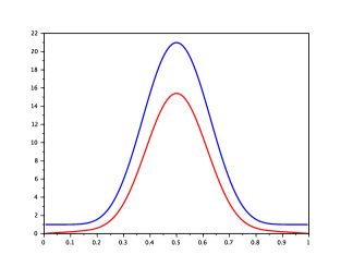
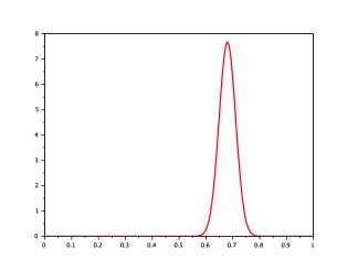
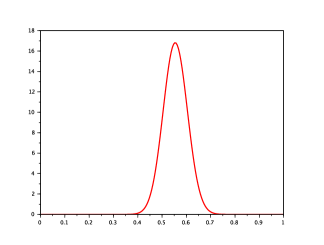
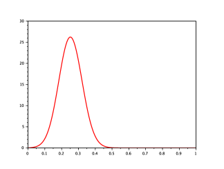
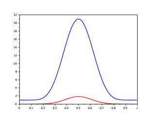
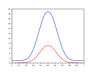
Figure 1: Snapshots of the evolution of the dispersal for three different times according to the parabolic problem (28). Top figures depict the space repartition $\rho(x)$ (fixed blue curve = $K$, increasing red = $\rho$). Bottom figures depict the trait distribution $\int_{0}^{1}n(x,\theta,t)dx$.

Some numerics on the parabolic problem.

Numerical simulations are presented in Figure 1 which illustrates the selection of lowest dispersal rate. Considering the parabolic problem (28), that means the convergence of the fittest trait $\bar{\theta}(t)$ to the smaller values of the trait (with the coefficients below, this value is $\theta=0$) as $t\to\infty$.

For this simulation we have chosen $\Omega=(0,1)$ and the data

$$D(\theta)=1.5\;\theta,\qquad K(x)=1+20\big{(}1-4(x-.5)^{2}\big{)}^{8},$$

and we have used, for the convenience of numerics, Dirichlet boundary conditions both in $x$ and $\theta$. The numerical scheme is the standard three points scheme in each direction, implicit in $x$ and explicit in $\theta$ because $\varepsilon=10^{-2}$ is small enough so as not to penalize the computational time.

In Figure 1, we observe that the average trait, which initially is $\theta\sim 0.7$, decreases and gets close to $0$ at the third time displayed here, also the trait exhibits a concentrated pattern around its average.

References

• [1] A. Arnold, L. Desvillettes and C. Prévost. Existence of nontrivial steady states for populations structured with respect to space and a continuous trait, Commun. Pure Appl. Anal. 11, 83–96, 2012.
• [2] M. Baar, A. Bovier and N. Champagnat. From stochastic, individual-based models to the canonical equation of adaptive dynamics - in one step. arXiv:1505.02421, 2015. To appear in Ann. Appl. Probab.
• [3] H. Berestycki, B. Nicolaenko, and B. Scheurer. Traveling wave solutions to combustion models and their singular limits, SIAM J. Math. Anal., 16 (1985), 1207–1242.
• [4] H. Berestycki, T. Jin and L. Silvestre. Propagation in a nonlocal reaction diffusion equation with spatial and genetic trait structure. arXiv:1411.2019, 2014. To appear in Nonlinearity.
• [5] N. Berestycki, C. Mouhot, G. Raoul, Existence of self-accelerating fronts for a non-local reaction-diffusion equation. ArXiv:1512.00903, (2015).
• [6] E. Bouin, V. Calvez, Travelling waves for the cane toads equation with bounded traits, Nonlinearity 27(9), 2233, 2014. Doi:10.1088/0951-7715/27/9/2233.
• [7] E. Bouin, V. Calvez, Propagation in a Kinetic Reaction-Transport Equation: Travelling Waves And Accelerating Fronts. Archive for Rational Mechanics and Analysis, 217(2), 571–617, 2015.
• [8] E. Bouin, V. Calvez, N. Meunier, S. Mirrahimi, B. Perthame, G. Raoul, and R. Voituriez. Invasion fronts with variable motility: phenotype selection, spatial sorting and wave acceleration. C. R. Math. Acad. Sci. Paris, 350(15-16):761–766, 2012.
• [9] E. Bouin and S. Mirrahimi. A Hamilton-Jacobi limit for a model of population structured by space and trait. Comm. Math Sci., 13(6): 1431–1452, 2015.
• [10] F. Campillo and C. Fritsch. Weak convergence of a mass-structured individual-based model. Applied Mathematics & Optimization, Vol. 72 (2015), no. 1, 37–73.
• [11] R. S. Cantrell, C. Cosner, Y. Lou. Approximating the ideal free distribution via reaction- diffusion-advection equations. J. Differential Equations, 245 (2008), no. 12, 36873703.
• [12] N. Champagnat, R. Ferrière, and S. Méléard. Unifying evolutionary dynamics: From individual stochastic processes to macroscopic models. Th. Pop. Biol., 69(3):297–321, 2006.
• [13] C. Cosner, J. Dávila J. and S. Martínez. Evolutionary stability of ideal free nonlocal dispersal. J. Biol. Dyn., Vol. 6 (2012), No. 2, 395405.
• [14] J. Coville and L. Dupaigne. Propagation speed of travelling fronts in non local reaction- diffusion equations, Nonlin. Anal., 60 (2005), 797–819.
• [15] L. Desvillettes, P.-E. Jabin, S. Mischler, and G. Raoul. On selection dynamics for continuous structured populations. Comm. Math. Sci. 6(3), 729–747 (2008).
• [16] O. Diekmann, A beginner’s guide to adaptive dynamics. In Rudnicki, R. (Ed.), Mathematical modeling of population dynamics, Banach Center Publications ,Vol. 63, (2004) 47–86.
• [17] O. Diekmann, P.-E. Jabin, S. Mischler, and B. Perthame. The dynamics of adaptation: an illuminating example and a Hamilton-Jacobi approach. Th. Pop. Biol., 67(4):257–271, 2005.
• [18] J. Dockery, V. Hutson, K. Mischaikow and M. Pernarowski. The evolution of slow dispersal rates: a reaction diffusion model. J. Math. Biol. (1998) 37: 61–83.
• [19] L. C. Evans. The perturbed test function method for viscosity solutions of nonlinear PDE. Proc. Roy. Soc. Edinburgh, 111 A (1989), 359–375.
• [20] S. A. H. Geritz, J. A. J. Metz , E. Kisdi and G. Meszena. Dynamics of adaptation and evolutionary branching. Physical Review Letters 78 (1997) 2024–2027.
• [21] R. Hambrock and Y. Lou. The evolution of conditional dispersal strategies in spatially hetero- geneous habitats. Bull. Math. Biol. 71 (2009), no. 8, 17931817.
• [22] A. Hastings. Can spatial variation alone lead to selection for dispersal? Theoret. Popul. Biol., 24 (1983), 244–251.
• [23] J. Hofbauer and K. Sigmund, Evolutionary games and population dynamics. London Mathematical Society, Student texts 7. Cambridge University Press (2002).
• [24] V. Hutson, S. Martínez, K. Mischaikow, G. T. Vickers. The evolution of dispersal, J. Math. Biol., 47 (2003), 6, 483–517.
• [25] P.-E. Jabin and G. Raoul. Selection dynamics with competition. J. Math. Biol., (2011) 63(3) 493–517.
• [26] K.-Y. Lam and Y. Lou. A mutation-selection model for evolution of random dispersal. ArXiv 1506.00662, 2015.
• [27] P.-L. Lions. Neumann type boundary conditions for Hamilton-Jacobi equations, Duke Math. J., 52 (1985), 793–820.
• [28] A. Lorz, S. Mirrahimi, and B. Perthame. Dirac mass dynamics in multidimensional nonlocal parabolic equations. Comm. Partial Differential Equations, 36(6):1071–1098, 2011.
• [29] Maynard Smith, J. The theory of games and the evolution of animal conflicts, J. Theor. Biol. 47 (1974), 209–221.
• [30] S. Mirrahimi and B. Perthame. Asymptotic analysis of a selection model with space. J. Math. Pures et Appl. 104 (2015) 1108–1118.
• [31] S. Mirrahimi and J.-M. Roquejoffre. Uniqueness in a class of Hamilton-Jacobi equations with constraints. Comptes Rendus Ac. Sc. Paris, Mathematiques, Vol. 353, (2015), 489–494: http://dx.doi.org/10.1016/j.crma.2015.03.005
• [32] S. Mirrahimi and J.-M. Roquejoffre. A class of Hamilton-Jacobi equations with constraint: uniqueness and constructive approach. Journal of Differential Equations, Vol. 260(5), 2016, 4717–4738.
• [33] K. Parvinen, U. Dieckmann, M. Gyllenberg and J. A. J. Metz. Evolution of dispersal in metapopulations with local density dependence and demographic stochasticity, J. Evol. Biol., (2003) 16:143–53.
• [34] B. Perthame and G. Barles. Dirac concentrations in Lotka-Volterra parabolic PDEs. Indiana Univ. Math. J., 57(7):3275–3301, 2008.
• [35] A. Potapov, U. E. Schlägel and M. A. Lewis. Evolutionary stable diffusive dispersal, DCDS(B), 19(10), 2014, 3319–3340.
• [36] O. Ronce. How does it feel to be like a rolling stone? Ten questions about dispersal evolution. Annu. Rev. Ecol. Evol. Syst., (2007) 38:231–253.
• [37] O. Turanova. On a model of a population with variable motility. Mathematical Models and Methods in Applied Sciences, Vol. 25, No. 10, 1961–2014 (2015).