B-meson spectroscopy in HQET at order 1/m1𝑚1/m

Fabio Bernardoni    BenoĂźt Blossier    John Bulava    Michele Della Morte    Patrick Fritzsch    Nicolas Garron    Antoine GĂ©rardin    Jochen Heitger    Georg von Hippel    Hubert Simma
Abstract

We present a study of the B spectrum performed in the framework of Heavy Quark Effective Theory expanded to next-to-leading order in 1/mb1subscript𝑚b1/m_{\rm b} and non-perturbative in the strong coupling. Our analyses have been performed on Nf=2subscript𝑁f2N_{\rm f}=2 lattice gauge field ensembles corresponding to three different lattice spacings and a wide range of pion masses. We obtain the BssubscriptBs{\rm B}_{\rm s}-meson mass and hyperfine splittings of the B- and BssubscriptBs{\rm B}_{\rm s}-mesons that are in good agreement with the experimental values and examine the mass difference mBs−mBsubscript𝑚subscriptBssubscript𝑚Bm_{{\rm B}_{\rm s}}-m_{\rm B} as a further cross-check of our previous estimate of the b-quark mass. We also report on the mass splitting between the first excited state and the ground state in the B and BssubscriptBs{\rm B}_{\rm s} systems.

1 Introduction

Lattice studies of the hadron spectrum provide valuable indications on the reliability of effective field theories. A phenomenologically relevant example is given by effective field theories for heavy quarks, such as Heavy Quark Effective Theory (HQET) or Non-Relativistic QCD (NRQCD). In this respect, hyperfine splittings are of great theoretical interest, since they vanish in the static (1/mh→∞→1subscript𝑚h1/m_{\rm h}\to\infty) limit, and thus serve to probe subleading terms in the heavy quark expansion.

Regarding specifically the hyperfine splitting of the B spectrum, it is well known that the masses of the pseudoscalar BqsubscriptB𝑞{\rm B}_{q} and vector Bq∗subscriptsuperscriptB𝑞\mathrm{B}^{*}_{q} differ as a result of spin effects [1]. This mass difference is produced in HQET by a O​(1/mh)O1subscript𝑚h{\rm O}(1/m_{\rm h}) chromomagnetic term in the Lagrangian that breaks the heavy quark spin symmetry of the static theory [2, 3]. In the context of lattice NRQCD it was found that in order to obtain a determination of the hyperfine splittings of bottomonium that is consistent with experiments, the perturbative improvement of the NRQCD action to at least one-loop order is required [4, 5, 6], for values of the lattice spacing of about 0.1 fm. The ΄΄\Upsilon spectrum, on the other hand, is well reproduced within NRQCD, and has been used in the literature as a quantity to set the lattice spacing [7, 8]. Hyperfine splittings have also been studied within the HISQ approach to heavy quarks [9].

In contrast to other studies, our results are based on non-perturbatively renormalized HQET including the next-to-leading order terms in the inverse heavy quark mass expansion. When formulated with a lattice regulator, the resulting lattice field theory can be non-perturbatively matched to QCD in the continuum limit. This provides a rigorous and systematically improvable approach to the study of the B-meson system.

Although permil precision seems difficult to reach within this approach, as it would require including 1/mh21superscriptsubscript𝑚h21/m_{\rm h}^{2} corrections, the control over systematics such as the non-perturbative subtraction of power-divergences and the related existence of the continuum limit, makes the approach very appealing and conceptually sound and in this sense, and in our view, more precise than other methods. In addition, as evident in [10] and emphasized in [11], for quantities more “complicated” than decay constants, such as form-factors, there is great need for results from different approaches, with different levels of control on the various systematics. Applications of the non-perturbative HQET formalism to form-factors are well on their way [12, 13, 14].

Remaining within spectrum-related observables, another quantity of interest is the SU(3) isospin breaking difference mBs−mBsubscript𝑚subscriptBssubscript𝑚Bm_{{\rm B}_{\rm s}}-m_{\rm B}. Most of the dependence on the heavy quark mass cancels in the difference and the statistical correlations between the strange and light-quark measurements should lead to a much improved precision in the determination of the difference compared to what would be possible for the individual masses. In [15], the mass of the B-meson has been used to determine the b-quark mass. Since the mass of the BssubscriptBs{\rm B}_{\rm s}-meson could have equally well been used, it is instructive to study how the strange-light mass difference propagates to the b-quark mass measurement.

Relatively little is known experimentally on the radial excitations of B-mesons, usually denoted by Bâ€ČsuperscriptBâ€Č\mathrm{B}^{\prime}. CDF has claimed the observation of a resonant state B​(5970)B5970{\rm B}(5970) that may be interpreted as a Bâ€ČsuperscriptBâ€Č\mathrm{B}^{\prime} state [16]. Lattice predictions for the radial excitation energies of the B system have been made in the framework of NRQCD [17, 18] and HQET [19, 20, 21, 22, 23, 24, 25, 26, 27], but, with the exception of the most recent HQET studies, control of the continuum extrapolation has been limited, if possible at all. An additional difficulty that always needs to be addressed is in disentangling single particle excitations from multi-particle states. We use the notation BrsuperscriptBr{\rm B}^{\rm r} (or BqrsubscriptsuperscriptBr𝑞{\rm B}^{\rm r}_{q} with q=u/d𝑞udq={\rm u}/{\rm d} or ss{\rm s}) for the excited states that we observe. They might be identified with radial excitations Bâ€ČsuperscriptBâ€Č\mathrm{B}^{\prime}, but without a dedicated study including also multi-hadron operators, we are unable to conclusively determine the nature of these excited states.

In this paper, we report on our estimate of the hyperfine splitting mB∗−mBsubscript𝑚superscriptBsubscript𝑚Bm_{\rm B^{*}}-m_{\rm B} in the B and BssubscriptBs{\rm B}_{\rm s} systems, and on the mass differences mBr−mBsubscript𝑚superscriptBrsubscript𝑚Bm_{{\rm B}^{\rm r}}-m_{\rm B}, mBsr−mBssubscript𝑚subscriptsuperscriptBrssubscript𝑚subscriptBsm_{{\rm B}^{\rm r}_{\rm s}}-m_{{\rm B}_{\rm s}} and mBs−mBsubscript𝑚subscriptBssubscript𝑚Bm_{{\rm B}_{\rm s}}-m_{\rm B} from Nf=2subscript𝑁f2N_{\rm f}=2 lattice simulations.

2 Theoretical setup

2.1 HQET on the lattice

The HQET action at O​(1/mh)O1subscript𝑚h{\rm O}(1/m_{\rm h}) reads

SHQETsubscript𝑆HQET\displaystyle S_{\rm HQET} =a4​∑x{ℒstat​(x)−ωkin​đ’Șkin​(x)−ωspin​đ’Șspin​(x)},absentsuperscript𝑎4subscriptđ‘„subscriptℒstatđ‘„subscript𝜔kinsubscriptđ’Șkinđ‘„subscript𝜔spinsubscriptđ’Șspinđ‘„\displaystyle=a^{4}{\sum}_{x}\big{\{}{\mathscr{L}}_{\rm stat}(x)-\omega_{\rm kin}\mathcal{O}_{\rm kin}(x)-\omega_{\rm spin}\mathcal{O}_{\rm spin}(x)\big{\}}\,, (2.1)
ℒstat​(x)subscriptℒstatđ‘„\displaystyle{\mathscr{L}}_{\rm stat}(x) =ÏˆÂŻh​(x)​D0​ψh​(x),absentsubscript¯𝜓hđ‘„subscriptđ·0subscript𝜓hđ‘„\displaystyle=\overline{\psi}_{\rm h}(x)\,D_{0}\,\psi_{\rm h}(x)\,, (2.2)
đ’Șkin​(x)subscriptđ’Șkinđ‘„\displaystyle\mathcal{O}_{\rm kin}(x) =ÏˆÂŻh​(x)​𝐃2​ψh​(x),absentsubscript¯𝜓hđ‘„superscript𝐃2subscript𝜓hđ‘„\displaystyle=\overline{\psi}_{\rm h}(x)\,{\bf D}^{2}\,\psi_{\rm h}(x)\,, (2.3)
đ’Șspin​(x)subscriptđ’Șspinđ‘„\displaystyle\mathcal{O}_{\rm spin}(x) =ÏˆÂŻh​(x)â€‹đˆâ‹…đâ€‹Ïˆh​(x),absent⋅subscript¯𝜓hđ‘„đˆđsubscript𝜓hđ‘„\displaystyle=\overline{\psi}_{\rm h}(x)\,\mbox{\boldmath$\sigma$}\cdot{\bf B}\,\psi_{\rm h}(x)\,, (2.4)

where the subscript hh\rm h denotes a heavy (static) quark field satisfying 1+Îł02​ψh=ψh1subscriptđ›Ÿ02subscript𝜓hsubscript𝜓h\frac{1+\gamma_{0}}{2}\psi_{\rm h}=\psi_{\rm h}, and the operators are normalized such that the classical (tree level) values of the coefficients are ωkin=ωspin=1/(2​mh)subscript𝜔kinsubscript𝜔spin12subscript𝑚h\omega_{\rm kin}=\omega_{\rm spin}=1/(2m_{\rm h}). The energy levels computed in this theory are relative to a bare mass mbaresubscript𝑚barem_{\rm bare}, which at tree level is simply mhsubscript𝑚hm_{\rm h}, but has to absorb a power-divergent shift at the quantum level, implying that it will take a different value depending on whether the O​(1/mh)O1subscript𝑚h{\rm O}(1/m_{\rm h}) terms are included or not.

ÎČ=5.5đ›œ5.5\beta=5.5 ÎČ=5.3đ›œ5.3\beta=5.3 ÎČ=5.2đ›œ5.2\beta=5.2
HYP1 HYP2 HYP1 HYP2 HYP1 HYP2
a​mbarestat𝑎superscriptsubscript𝑚barestatam_{\rm bare}^{\rm stat} 0.969​(12)0.969120.969(12) 1.000​(12)1.000121.000(12) 1.317​(15)1.317151.317(15) 1.350​(15)1.350151.350(15) 1.520​(17)1.520171.520(17) 1.553​(17)1.553171.553(17)
a​mbare𝑎subscript𝑚baream_{\rm bare} 0.594​(14)0.594140.594(14) 0.606​(14)0.606140.606(14) 0.993​(17)0.993170.993(17) 1.014​(17)1.014171.014(17) 1.214​(18)1.214181.214(18) 1.239​(18)1.239181.239(18)
ωkin/asubscript𝜔kin𝑎\omega_{\rm kin}/a 0.520​(11)0.520110.520(11) 0.525​(10)0.525100.525(10) 0.415​(8)0.41580.415(8) 0.418​(8)0.41880.418(8) 0.377​(7)0.37770.377(7) 0.380​(7)0.38070.380(7)
ωspin/asubscript𝜔spin𝑎\omega_{\rm spin}/a 0.949​(37)0.949370.949(37) 1.090​(42)1.090421.090(42) 0.73​(28)0.73280.73(28) 0.883​(33)0.883330.883(33) 0.655​(24)0.655240.655(24) 0.812​(30)0.812300.812(30)
Table 1: Values of HQET parameters at the physical point 𝝎​(z=zb)𝝎𝑧subscript𝑧b\boldsymbol{\omega}(z=z_{{\rm b}}). As determined in [15], we have used zbstat=13.24superscriptsubscript𝑧bstat13.24z_{{\rm b}}^{\rm stat}=13.24 to interpolate the parameters of HQET at static order, and zb=13.25subscript𝑧b13.25z_{{\rm b}}=13.25 for the parameters of HQET expanded to NLO. The bare coupling g0subscript𝑔0g_{0} is given by ÎČ=6/g02đ›œ6superscriptsubscript𝑔02\beta=6/g_{0}^{2}.

The renormalizability of the static theory can be preserved at NLO by considering a strict expansion of correlation functions in 1/mh1subscript𝑚h1/m_{\rm h},

⟹O⟩=⟹O⟩stat+ωkin​a4​∑x⟹O​đ’Șkin​(x)⟩stat+ωspin​a4​∑x⟹O​đ’Șspin​(x)⟩stat,delimited-âŸšâŸ©đ‘‚subscriptdelimited-âŸšâŸ©đ‘‚statsubscript𝜔kinsuperscript𝑎4subscriptđ‘„subscriptdelimited-âŸšâŸ©đ‘‚subscriptđ’Șkinđ‘„statsubscript𝜔spinsuperscript𝑎4subscriptđ‘„subscriptdelimited-âŸšâŸ©đ‘‚subscriptđ’Șspinđ‘„stat\langle O\rangle=\langle O\rangle_{\rm stat}+\omega_{\rm kin}\,a^{4}{\sum}_{x}\langle O\,\mathcal{O}_{\rm kin}(x)\rangle_{\rm stat}+\omega_{\rm spin}\,a^{4}{\sum}_{x}\langle O\,\mathcal{O}_{\rm spin}(x)\rangle_{\rm stat}\;, (2.5)

where the suffix “stat” denotes an expectation value measured in the static theory.

The values of the parameters mbarestatsuperscriptsubscript𝑚barestatm_{\rm bare}^{\rm stat} and {mbare,ωkin,ωspin}subscript𝑚baresubscript𝜔kinsubscript𝜔spin\left\{m_{\rm bare},\omega_{\rm kin},\omega_{\rm spin}\right\} required to match to QCD have been determined in [28, 15] using the Schrödinger Functional scheme. In order to keep this paper self-contained, we summarize in Table 1 their values for the three lattice spacings a​(ÎČ)đ‘Žđ›œa(\beta) and two static discretizations (HYP1, HYP2 [29]) that we use. The parameters are given at zb=L1​Mbsubscript𝑧bsubscript𝐿1subscript𝑀bz_{\rm b}=L_{1}M_{\rm b} where Mbsubscript𝑀bM_{\rm b} is the Renormalization Group Invariant (RGI) b-quark mass and L1subscript𝐿1L_{1} is the linear extent of the lattice used for the matching.

2.2 The variational method

For spectroscopic applications, having good control over contributions from excited states is crucial to reduce the systematic error on the determination of the ground state. For this purpose it is necessary to use a variational method [30, 31, 32, 33, 34], which starts from matrices of correlation functions,

Ci​jstat​(t)subscriptsuperscriptđ¶stat𝑖𝑗𝑡\displaystyle C^{\rm{stat}}_{ij}(t) =\displaystyle= ∑x,đČ⟹Oi​(x0+t,đČ)​Oj∗​(x)⟩stat,subscriptđ‘„đČsubscriptdelimited-⟚⟩subscript𝑂𝑖subscriptđ‘„0𝑡đČsubscriptsuperscriptđ‘‚đ‘—đ‘„stat\displaystyle\sum_{x,\bf{y}}\left<O_{i}(x_{0}+t,{\bf y})\,O^{*}_{j}(x)\right>_{\rm stat}\,,
Ci​jkin/spin​(t)subscriptsuperscriptđ¶kinspin𝑖𝑗𝑡\displaystyle C^{\rm{kin/spin}}_{ij}(t) =\displaystyle= ∑x,đČ,z⟹Oi​(x0+t,đČ)​Oj∗​(x)​đ’Șkin/spin​(z)⟩stat,subscriptđ‘„đČ𝑧subscriptdelimited-⟚⟩subscript𝑂𝑖subscriptđ‘„0𝑡đČsubscriptsuperscriptđ‘‚đ‘—đ‘„subscriptđ’Șkinspin𝑧stat\displaystyle\sum_{x,{\bf y},z}\;\left<O_{i}(x_{0}+t,{\bf y})\,O^{*}_{j}(x)\,{\cal O}_{\rm kin/spin}(z)\right>_{\rm stat}\,,

containing all pairwise correlators of some set of interpolating fields Oi,i=1,
,Nformulae-sequencesubscript𝑂𝑖𝑖1
𝑁O_{i}\,,\;i=1,\ldots,N, and proceeds to solve the generalized eigenvalue problem (GEVP)

Cstat​(t)​vnstat​(t,t0)=λnstat​(t,t0)​Cstat​(t0)​vnstat​(t,t0),n=1,
,N,t>t0.formulae-sequencesuperscriptđ¶stat𝑡subscriptsuperscript𝑣stat𝑛𝑡subscript𝑡0subscriptsuperscript𝜆stat𝑛𝑡subscript𝑡0superscriptđ¶statsubscript𝑡0subscriptsuperscript𝑣stat𝑛𝑡subscript𝑡0formulae-sequence𝑛1
𝑁𝑡subscript𝑡0\displaystyle C^{\rm stat}(t)\,v^{\rm stat}_{n}(t,t_{0})=\lambda^{\rm stat}_{n}(t,t_{0})\,C^{\rm stat}(t_{0})\,v^{\rm stat}_{n}(t,t_{0})\,,\quad n=1,\ldots,N\,,\quad t>t_{0}\;. (2.7)

From the generalized eigenvalues λnstat​(t,t0)superscriptsubscript𝜆𝑛stat𝑡subscript𝑡0\lambda_{n}^{\rm stat}(t,t_{0}) and the corresponding eigenvectors vnstat​(t,t0)superscriptsubscript𝑣𝑛stat𝑡subscript𝑡0v_{n}^{\rm stat}(t,t_{0}), the effective energy levels can be computed as [34, 35]

Eneff,stat​(t,t0)superscriptsubscript𝐾𝑛effstat𝑡subscript𝑡0\displaystyle E_{n}^{\rm eff,{\rm stat}}(t,t_{0}) =−1a​[log⁥λnstat​(t+a,t0)−log⁥λnstat​(t,t0)],absent1𝑎delimited-[]superscriptsubscript𝜆𝑛stat𝑡𝑎subscript𝑡0superscriptsubscript𝜆𝑛stat𝑡subscript𝑡0\displaystyle=-{1\over a}\,[\log{\lambda_{n}^{\rm stat}(t+a,t_{0})}-\log{\lambda_{n}^{\rm stat}(t,t_{0})}]\,,
Eneff,x​(t,t0)superscriptsubscript𝐾𝑛effx𝑡subscript𝑡0\displaystyle E_{n}^{\rm eff,x}(t,t_{0}) =λnx​(t,t0)λnstat​(t,t0)−λnx​(t+a,t0)λnstat​(t+a,t0),absentsuperscriptsubscript𝜆𝑛x𝑡subscript𝑡0superscriptsubscript𝜆𝑛stat𝑡subscript𝑡0superscriptsubscript𝜆𝑛x𝑡𝑎subscript𝑡0superscriptsubscript𝜆𝑛stat𝑡𝑎subscript𝑡0\displaystyle={\lambda_{n}^{\rm x}(t,t_{0})\over\lambda_{n}^{\rm stat}(t,t_{0})}\,-\,{\lambda_{n}^{\rm x}(t+a,t_{0})\over\lambda_{n}^{\rm stat}(t+a,t_{0})}\,, (2.8)

where x∈{kin,spin}xkinspin{\rm x}\in\{{\rm kin},{\rm spin}\} and

λnx​(t,t0)λnstat​(t,t0)superscriptsubscript𝜆𝑛x𝑡subscript𝑡0superscriptsubscript𝜆𝑛stat𝑡subscript𝑡0\displaystyle{\lambda_{n}^{\rm x}(t,t_{0})\over\lambda_{n}^{\rm stat}(t,t_{0})} =(vnstat​(t,t0),[[λnstat​(t,t0)]−1​Cx​(t)−Cx​(t0)]​vnstat​(t,t0)).absentsuperscriptsubscript𝑣𝑛stat𝑡subscript𝑡0delimited-[]superscriptdelimited-[]superscriptsubscript𝜆𝑛stat𝑡subscript𝑡01superscriptđ¶x𝑡superscriptđ¶xsubscript𝑡0superscriptsubscript𝑣𝑛stat𝑡subscript𝑡0\displaystyle=\left(v_{n}^{\rm stat}(t,t_{0})\,,\,[[\lambda_{n}^{\rm stat}(t,t_{0})]^{-1}\,C^{\rm x}(t)-C^{\rm x}(t_{0})]v_{n}^{\rm stat}(t,t_{0})\right)\,. (2.9)

The corresponding asymptotic behaviour is known to be

Eneff,stat​(t,t0)superscriptsubscript𝐾𝑛effstat𝑡subscript𝑡0\displaystyle E_{n}^{\rm eff,{\rm stat}}(t,t_{0}) =Enstat+ÎČnstat​e−Δ​EN+1,nstat​t+
,absentsuperscriptsubscript𝐾𝑛statsuperscriptsubscriptđ›œđ‘›statsuperscripteΔsuperscriptsubscript𝐾𝑁1𝑛stat𝑡
\displaystyle=E_{n}^{\rm stat}\,+\,\beta_{n}^{\rm stat}\,{\rm e}^{-\Delta E_{N+1,n}^{\rm stat}\,t}+\ldots\,, (2.10)
Eneff,x​(t,t0)superscriptsubscript𝐾𝑛effx𝑡subscript𝑡0\displaystyle E_{n}^{\rm eff,x}(t,t_{0}) =Enx+[ÎČnx−ÎČnstat​t​Δ​EN+1,nx]​e−Δ​EN+1,nstat​t+
,absentsuperscriptsubscript𝐾𝑛xdelimited-[]superscriptsubscriptđ›œđ‘›xsuperscriptsubscriptđ›œđ‘›stat𝑡Δsuperscriptsubscript𝐾𝑁1𝑛xsuperscripteΔsuperscriptsubscript𝐾𝑁1𝑛stat𝑡
\displaystyle=E_{n}^{\rm x}\,+\,[\,\beta_{n}^{\rm x}\,-\,\beta_{n}^{\rm stat}\,t\,\Delta E_{N+1,n}^{\rm x}\,]{\rm e}^{-\Delta E_{N+1,n}^{\rm stat}\,t}+\ldots\,,\qquad (2.11)

where the energy gap is defined as Δ​Em,n=Em−EnΔsubscript𝐾𝑚𝑛subscript𝐾𝑚subscript𝐾𝑛\Delta E_{m,n}=E_{m}-E_{n}.

In our study, the operator basis used is given by heavy-light bilinears with varying levels of Gaussian smearing [36] applied to the light quark field,

Ok​(x)subscriptđ‘‚đ‘˜đ‘„\displaystyle O_{k}(x) =ÏˆÂŻh​(x)​γ0​γ5​ψq(k)​(x),absentsubscript¯𝜓hđ‘„subscriptđ›Ÿ0subscriptđ›Ÿ5superscriptsubscriptđœ“đ‘žđ‘˜đ‘„\displaystyle=\overline{\psi}_{\rm h}(x)\,\gamma_{0}\gamma_{5}\,\psi_{q}^{(k)}(x)\,, ψq(k)​(x)superscriptsubscriptđœ“đ‘žđ‘˜đ‘„\displaystyle\psi_{q}^{(k)}(x) =(1+ÎșG​a2​Δ)Rk​ψq​(x),absentsuperscript1subscript𝜅Gsuperscript𝑎2Δsubscript𝑅𝑘subscriptđœ“đ‘žđ‘„\displaystyle=\left(1+\kappa_{\rm G}\,a^{2}\,\Delta\right)^{R_{k}}\psi_{q}(x)\,, (2.12)

where q=u/d𝑞udq={\rm u}/{\rm d} or ss{\rm s}. The covariant Laplacian ΔΔ\Delta is built from gauge links that have been triply APE smeared [37, 38] in the spatial directions, and the smearing parameters ÎșGsubscript𝜅G\kappa_{\rm G} and Rksubscript𝑅𝑘R_{k} are chosen so as to approximately cover the same sequence of physical radii at each value of the lattice spacing, as discussed in [15]. We solve the GEVP for the matrix of correlators in the static limit for N=3𝑁3N=3.

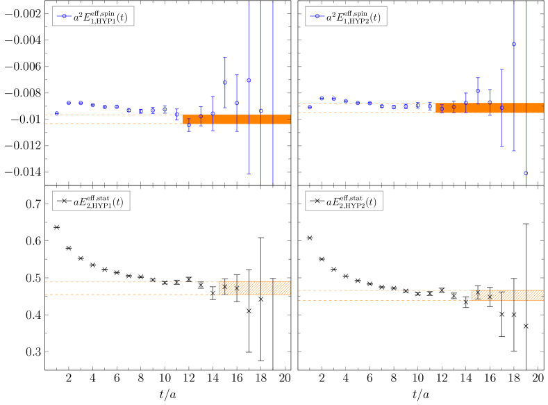
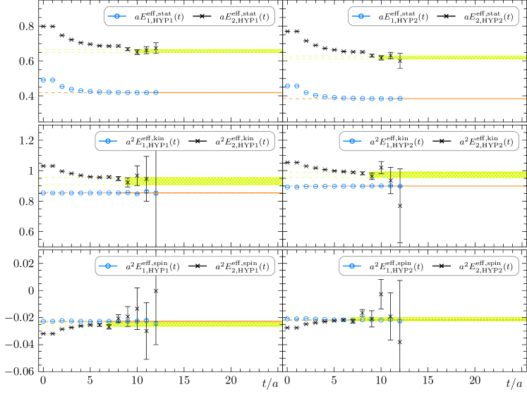
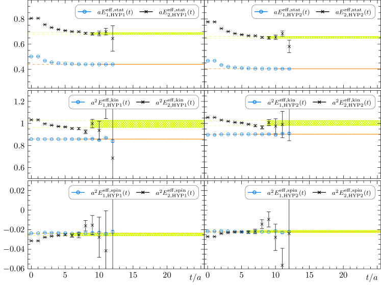
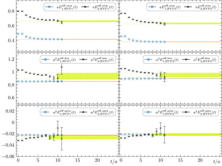
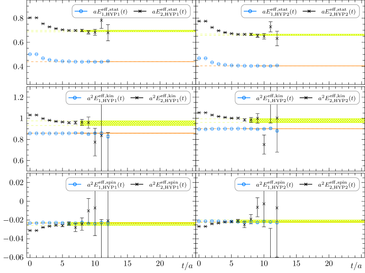
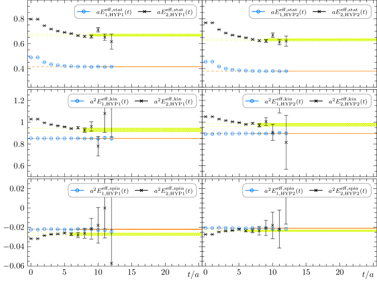
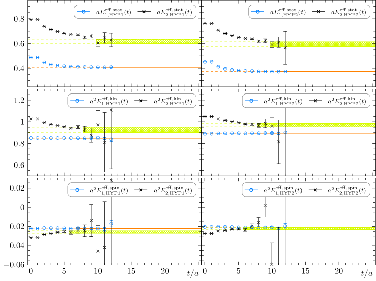
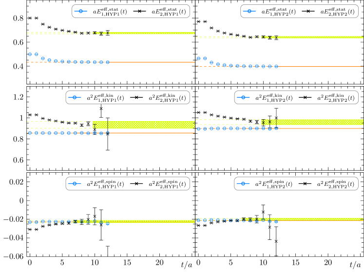
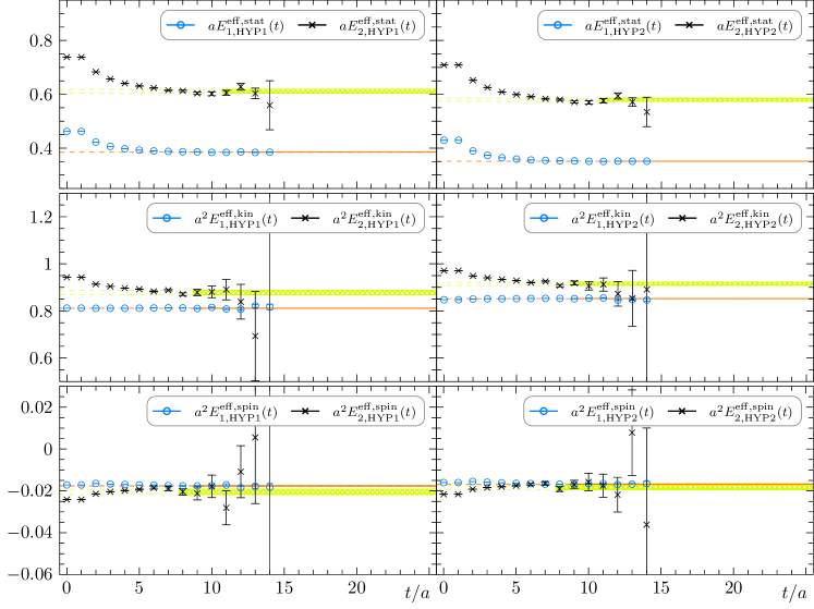
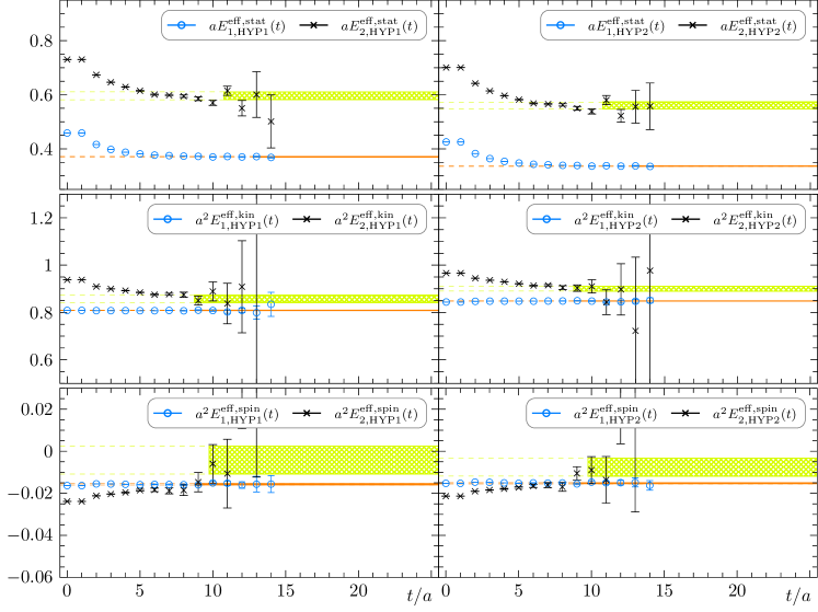
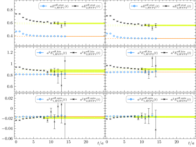
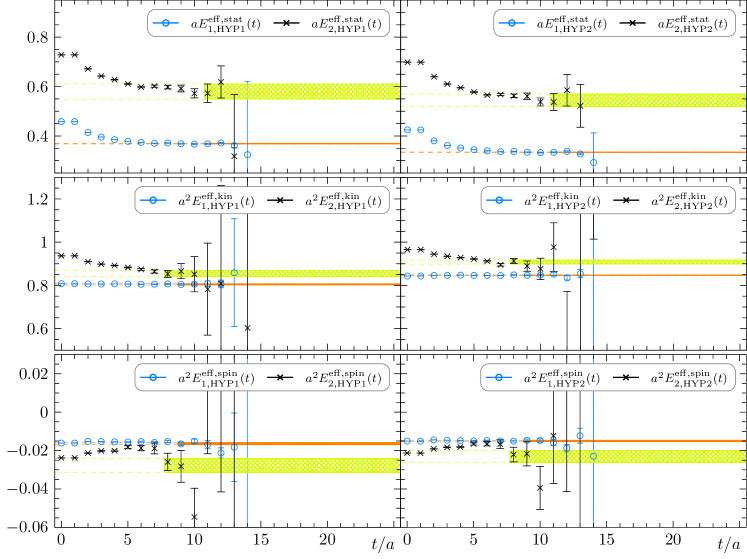
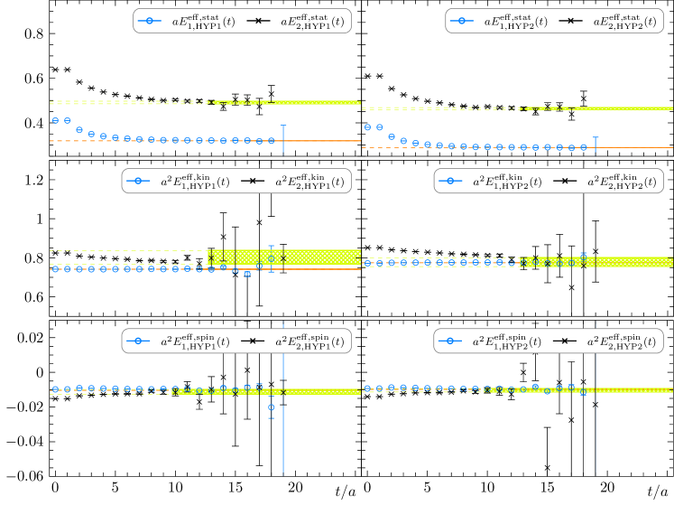
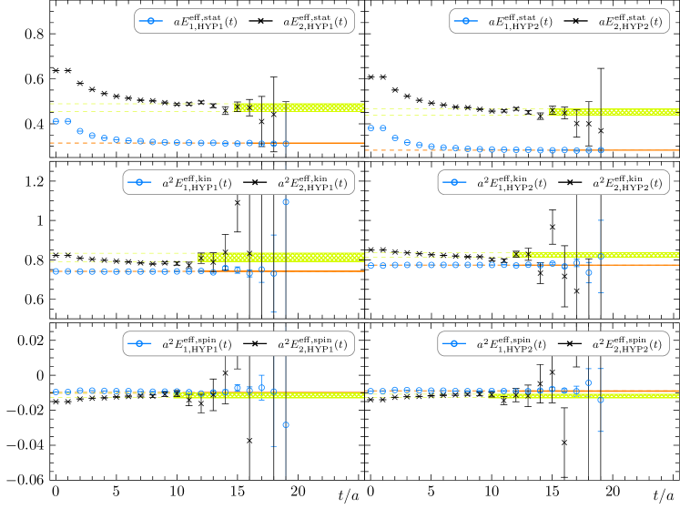
An illustration of two typical plateaux of the energies E1spinsuperscriptsubscript𝐾1spinE_{1}^{\rm spin} and E2statsuperscriptsubscript𝐾2statE_{2}^{\rm stat} is shown in Fig. 1.

Refer to caption
Figure 1: Illustration of typical plateaux for the O​(1/mb)O1subscript𝑚b{\rm O}(1/m_{\rm b}) chromomagnetic energy a2​E1spinsuperscript𝑎2subscriptsuperscript𝐾spin1a^{2}E^{\rm spin}_{1} (top) and the first excited state static energy a​E2stat𝑎subscriptsuperscript𝐾stat2aE^{\rm stat}_{2} (bottom), computed on the CLS ensemble N6 (a=0.048𝑎0.048a=0.048 fm, mπ=340subscript𝑚𝜋340m_{\pi}=340 MeV).

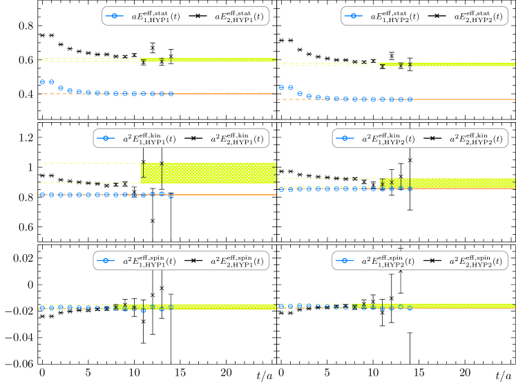
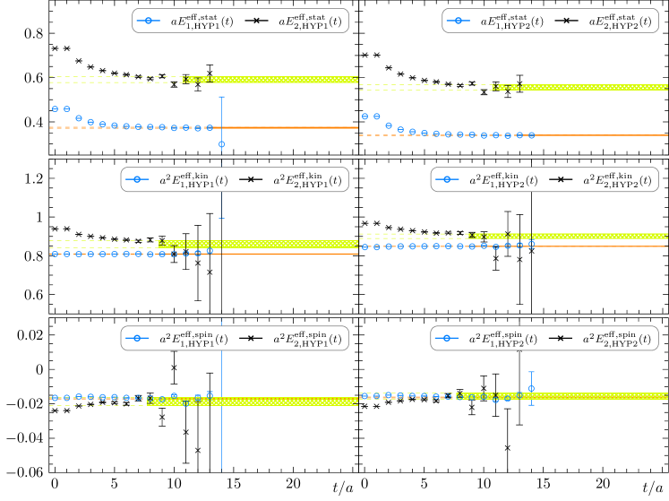
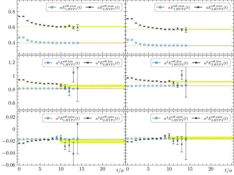
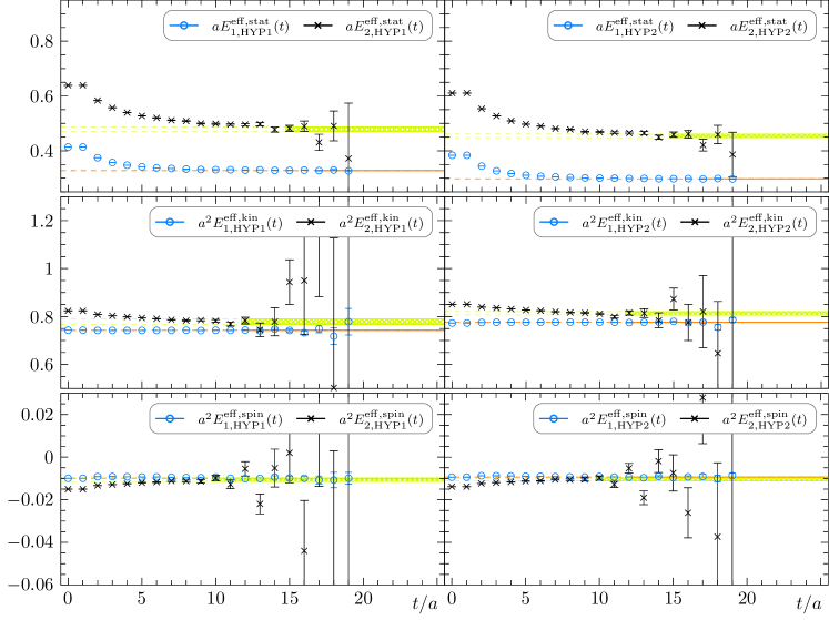
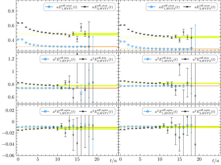
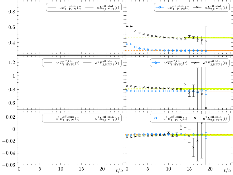
The plateau regions used for weighted averaging have been chosen by applying the procedure already discussed in [39, 40] in order to ensure that the systematic errors due to excited-state contributions are less than a given fraction (typically 1/3) of the statistical errors on the GEVP results. As a consistency check, we have also employed a global fit of the form of eqs. (2.10) and (2.11) to our data. The values of Ensubscript𝐾𝑛E_{n} obtained from the fit are compatible with the plateau values, and generally exhibit smaller statistical errors. We therefore consider our errors to be estimated conservatively.

2.3 Computing masses

We start by recalling the definition of the BqsubscriptB𝑞{\rm B}_{q}-meson mass as it has been used to non-perturbatively fix the HQET parameters for the static quark discretizations HYP1 and HYP2 in [15]. On the lattice one combines the HQET parameters (see Table 1, or [41] for a more detailed discussion) with the large volume computations of ground state energies,

mBqstat​(mπ,a)superscriptsubscript𝑚subscriptB𝑞statsubscript𝑚𝜋𝑎\displaystyle m_{{\rm B}_{q}}^{\rm stat}(m_{\pi},a) =mbarestat+E1stat|mq,absentsuperscriptsubscript𝑚barestatevaluated-atsuperscriptsubscript𝐾1statsubscript𝑚𝑞\displaystyle=m_{\rm bare}^{\rm stat}+E_{1}^{\rm stat}\big{|}_{m_{q}}\,, (2.13a)
mBq​(mπ,a)subscript𝑚subscriptB𝑞subscript𝑚𝜋𝑎\displaystyle m_{{\rm B}_{q}}(m_{\pi},a) =mbare+E1stat|mq+ωkin​E1kin|mq+ωspin​E1spin|mq.absentsubscript𝑚bareevaluated-atsuperscriptsubscript𝐾1statsubscript𝑚𝑞evaluated-atsubscript𝜔kinsuperscriptsubscript𝐾1kinsubscript𝑚𝑞evaluated-atsubscript𝜔spinsuperscriptsubscript𝐾1spinsubscript𝑚𝑞\displaystyle=m_{\rm bare}+E_{1}^{\rm stat}\big{|}_{m_{q}}+\omega_{\rm kin}E_{1}^{\rm kin}\big{|}_{m_{q}}+\omega_{\rm spin}E_{1}^{\rm spin}\big{|}_{m_{q}}\,. (2.13b)

We use the subscript mqsubscript𝑚𝑞m_{q} to indicate that the corresponding energy results from the GEVP analysis of correlation functions in the heavy-light (q=d𝑞dq={\rm d}) or heavy-strange (q=s𝑞sq={\rm s}) sector along the lines presented in Section 2.2. The PDG value mB=5.2795​GeVsubscript𝑚B5.2795GeVm_{\rm B}=5.2795\,{\rm GeV} in [1] has already been used as input to determine mbsubscript𝑚bm_{\rm b} [15] and thus the HQET parameters ωisubscript𝜔𝑖\omega_{i}. However, re-computing mBsubscript𝑚Bm_{\rm B} at fixed values of the HQET parameters serves as a non-trivial cross-check of our calculation. Additionally, we will compute mBssubscript𝑚subscriptBsm_{{\rm B}_{\rm s}} in the very same way. All remaining observables presented in the present paper are mass splittings which can be computed with the data resulting from our GEVP analysis. We now give their explicit definition before discussing any combined chiral and continuum extrapolation in Section 2.4.

The hyperfine splitting of the BqsubscriptB𝑞{\rm B}_{q}-meson system, mBq∗−mBqsubscript𝑚subscriptsuperscriptB𝑞subscript𝑚subscriptB𝑞m_{{\rm B}^{*}_{q}}-m_{{\rm B}_{q}}, is given by

ΔqHF​m​(mπ,a)subscriptsuperscriptΔHF𝑞𝑚subscript𝑚𝜋𝑎\displaystyle\Delta^{\rm HF}_{q}m\,(m_{\pi},a) =−43​ωspin​E1spin|mq,absentevaluated-at43subscript𝜔spinsuperscriptsubscript𝐾1spinsubscript𝑚𝑞\displaystyle=-\frac{4}{3}\omega_{\rm spin}E_{1}^{\rm spin}\big{|}_{m_{q}}\;, q𝑞\displaystyle q =s,d,absentsd\displaystyle={\rm s,d}\;, (2.14)

and depends on the HQET parameter ωspinsubscript𝜔spin\omega_{\rm spin} and the large-volume measurement of E1spinsuperscriptsubscript𝐾1spinE_{1}^{\rm spin}. The strange-light mass difference mBs−mBdsubscript𝑚subscriptBssubscript𝑚subscriptBdm_{{\rm B}_{\rm s}}-m_{{\rm B}_{\rm d}}, at the static and O​(1/mb)O1subscript𝑚b{\rm O}(1/m_{\rm b}) level, reads,

Δs−dstat​m​(mπ,a)superscriptsubscriptΔsdstat𝑚subscript𝑚𝜋𝑎\displaystyle\Delta_{\rm s-d}^{\rm stat}m\,(m_{\pi},a) =Δs−d​E1stat,absentsubscriptΔsdsuperscriptsubscript𝐾1stat\displaystyle=\Delta_{\rm s-d}E_{1}^{\rm stat}\,, (2.15a)
Δs−d​m​(mπ,a)subscriptΔsd𝑚subscript𝑚𝜋𝑎\displaystyle\Delta_{\rm s-d}m\,(m_{\pi},a) =Δs−d​E1stat+ωkin​Δs−d​E1kin+ωspin​Δs−d​E1spin,absentsubscriptΔsdsuperscriptsubscript𝐾1statsubscript𝜔kinsubscriptΔsdsuperscriptsubscript𝐾1kinsubscript𝜔spinsubscriptΔsdsuperscriptsubscript𝐾1spin\displaystyle=\Delta_{\rm s-d}E_{1}^{\rm stat}+\omega_{\rm kin}\Delta_{\rm s-d}E_{1}^{\rm kin}+\omega_{\rm spin}\Delta_{\rm s-d}E_{1}^{\rm spin}\,, (2.15b)

respectively, where we have defined the shorthand Δs−d​Q=Q|mq=ms−Q|mq=md.subscriptΔsd𝑄evaluated-at𝑄subscript𝑚𝑞subscript𝑚sevaluated-at𝑄subscript𝑚𝑞subscript𝑚d\Delta_{\rm s-d}Q=\left.Q\right|_{m_{q}=m_{{\rm s}}}-\left.Q\right|_{m_{q}=m_{{\rm d}}}\,. Finally, the mass gaps for excited states, mBqr−mBqsubscript𝑚subscriptsuperscriptBr𝑞subscript𝑚subscriptB𝑞m_{{\rm B}^{\rm r}_{q}}-m_{{\rm B}_{q}}, can be computed from Δ​Em,n=Em−EnΔsubscript𝐾𝑚𝑛subscript𝐾𝑚subscript𝐾𝑛\Delta E_{m,n}=E_{m}-E_{n} via

Δr,qstat​m​(mπ,a)subscriptsuperscriptΔstatr𝑞𝑚subscript𝑚𝜋𝑎\displaystyle\Delta^{\rm stat}_{{\rm r,}q}m\,(m_{\pi},a) =Δ​E2,1stat|mq,absentevaluated-atΔsuperscriptsubscript𝐾21statsubscript𝑚𝑞\displaystyle=\Delta E_{2,1}^{\rm stat}\big{|}_{m_{q}}\,, (2.16a)
Δr,q​m​(mπ,a)subscriptΔr𝑞𝑚subscript𝑚𝜋𝑎\displaystyle\Delta_{{\rm r,}q}m\,(m_{\pi},a) =Δ​E2,1stat|mq+ωkin​Δ​E2,1kin|mq+ωspin​Δ​E2,1spin|mq,absentevaluated-atΔsuperscriptsubscript𝐾21statsubscript𝑚𝑞evaluated-atsubscript𝜔kinΔsuperscriptsubscript𝐾21kinsubscript𝑚𝑞evaluated-atsubscript𝜔spinΔsuperscriptsubscript𝐾21spinsubscript𝑚𝑞\displaystyle=\Delta E_{2,1}^{\rm stat}\big{|}_{m_{q}}+\omega_{\rm kin}\Delta E_{2,1}^{\rm kin}\big{|}_{m_{q}}+\omega_{\rm spin}\Delta E_{2,1}^{\rm spin}\big{|}_{m_{q}}\,, (2.16b)

to static and O​(1/mb)O1subscript𝑚b{\rm O}(1/m_{\rm b}) accuracy, respectively. As any observable computed on the lattice, these quantities depend on the input parameters used in the simulation. The strange and bottom quark mass have been fixed to their physical value along the lines reported in [42, 15, 41], such that only the dependences on the light quark mass—here parameterized by mπsubscript𝑚𝜋m_{\pi}—and lattice spacing a𝑎a remain.

We have extracted the energies on a subset of gauge ensembles from the Coordinated Lattice Simulations (CLS) effort for Nf=2subscript𝑁f2N_{\rm f}=2.

e𝑒e-id ÎČđ›œ\beta Îșd=Îșseasubscript𝜅dsubscript𝜅sea\kappa_{\rm d}=\kappa_{\rm sea} Îșssubscript𝜅s\kappa_{\rm s} Ï„đœ\tau τcfgsubscript𝜏cfg\tau_{\rm cfg} τexpsubscript𝜏exp\tau_{\rm exp} heavy-light heavy-strange
HYP1 HYP2 HYP1 HYP2
A4 5.2 0.135900 0.1352850 2 8 106    1012 [1,1]     1000 [1,1]
A5c 0.135940 0.1352570 2 4 39    501 [1,1]     500 [1,1]
A5d    500 [1,1] – –
B6 0.135970 0.1352390 2 2 39    636 [1,1]     636 [1,1]
E5 5.3 0.136250 0.1357770 4 16 151    1000 [1,1]     1000 [1,1]
F6 0.136350 0.1357410 2 8 151    500 [1,1]     600 [1,1]
F7 0.136380 0.1357300 2 8 151    602 [100,1]     200 [1,2]
G8 0.136417 0.1357050 2 2 56    410 [1,1] – –
N5 5.5 0.136600 0.1362620 0.5 8 488    477 [300,1] – –
N6 0.136670 0.1362500 2 4 108    950 [2,2]     707 [100,2]
O7 0.136710 0.1362430 2 4 108    980 [1,1] – 490 [1,2]
Table 2: Measurement details for observables in the light- and strange-quark sector. For each ensemble we list the light- and strange-quark hopping parameter, the trajectory length Ï„đœ\tau, the distance of saved configurations τcfgsubscript𝜏cfg\tau_{\rm cfg} and the exponential autocorrelation time τexpsubscript𝜏exp\tau_{\rm exp} in MDU. For each individual static quark discretization we then specify Nmssubscript𝑁msN_{\rm ms} [m𝑚m,d𝑑d], i.e., the total number of measurements starting from the mthsuperscript𝑚thm^{\rm th} saved configuration using every dthsuperscript𝑑thd^{\rm th}. Note that for A5 we have two independent Monte-Carlo chains.

The parameters of the simulations and the statistics entering our analysis are collected in Table 1 of [15]. Remaining details of the measurements have been summarized in Table 2.111For the B6-ensemble a preliminary value of Îșssubscript𝜅s\kappa_{\rm s} has been used, which produces a bare subtracted quark mass which differs by about 1 MeV from the final one. The light quark is treated in a unitary setup with mπsubscript𝑚𝜋m_{\pi} in the range [190​MeV190MeV190\,{\rm MeV}, 440​MeV440MeV440\,{\rm MeV}], and the bare strange quark mass has been tuned on each CLS ensemble to its physical value by using the kaon decay constant fKsubscript𝑓Kf_{\rm K} to set the scale [42] and mK=494.2​MeVsubscript𝑚K494.2MeVm_{\rm K}=494.2\,{\rm MeV}. The lattice spacings are a/fm∈{0.048,0.065,0.075}𝑎fm0.0480.0650.075a/{\rm fm}\in\{0.048,0.065,0.075\} for ÎČ∈{5.5,5.3,5.2}đ›œ5.55.35.2\beta\in\{5.5,5.3,5.2\}, corresponding to the CLS ensemble ids N–O, E–G and A–B, respectively. All lattices have mπ​L≄4subscript𝑚𝜋𝐿4m_{\pi}L\geq 4, such that finite-volume effects are sufficiently exponentially suppressed at the level of accuracy we are working at.

Our data analysis takes into account correlations between different observables as well as intrinsic autocorrelations of the Hybrid Monte Carlo (HMC) algorithm resulting from slow modes in the simulation. As these contributions rapidly grow towards the continuum limit, it is mandatory to estimate and include a-priori unknown long-tail contributions from the autocorrelation function of each individual observable. Further details of our analysis method can be found in Appendix A.

2.4 Extrapolation to the physical point

To extrapolate our data to the continuum limit and to the physical point, we take expressions from heavy meson chiral perturbation theory (HMÏ‡đœ’\chiPT) if available, and a linear ansatz otherwise.

In the chiral regime, the mass of the B-meson can be extrapolated to the physical point using a functional form motivated by HMÏ‡đœ’\chiPT [43]. Defining a subtracted mass by removing the leading non-analytic (in the quark mass) term, viz.

mBq,ÎŽsub​(y,a)=mBq​(mπ,a)+cq​3​g^216​π​(mπ3fπ2−(mπexp)3(fπexp)2),subscriptsuperscript𝑚subsubscriptB𝑞𝛿𝑩𝑎subscript𝑚subscriptB𝑞subscript𝑚𝜋𝑎subscript𝑐𝑞3superscript^𝑔216𝜋superscriptsubscript𝑚𝜋3superscriptsubscript𝑓𝜋2superscriptsuperscriptsubscript𝑚𝜋exp3superscriptsuperscriptsubscript𝑓𝜋exp2m^{\rm sub}_{{\rm B}_{q},\delta}(y,a)=m_{{\rm B}_{q}}(m_{\pi},a)+c_{q}\frac{3\widehat{g}^{2}}{16\pi}\left(\frac{m_{\pi}^{3}}{f_{\pi}^{2}}-\frac{(m_{\pi}^{\rm exp})^{3}}{(f_{\pi}^{\rm exp})^{2}}\right)\;, (2.17)

with cq=1subscript𝑐𝑞1c_{q}=1 in HMÏ‡đœ’\chiPT at NLO for q=d𝑞dq={\rm d} but zero otherwise, the parameterization reads

mBq,ÎŽsub​(y,a)=Bq+Cq​(y−yexp)+Dq,ή​a2.subscriptsuperscript𝑚subsubscriptB𝑞𝛿𝑩𝑎subscriptđ”đ‘žsubscriptđ¶đ‘žđ‘Šsuperscript𝑩expsubscriptđ·đ‘žđ›żsuperscript𝑎2m^{\rm sub}_{{\rm B}_{q},\delta}(y,a)=B_{q}+C_{q}\left(y-y^{\rm exp}\right)+D_{q,\delta}a^{2}\,. (2.18)

In (2.17) the B∗​B​πsuperscriptđ”đ”đœ‹B^{*}\!B\pi-coupling g^=0.492​(29)^𝑔0.49229\widehat{g}=0.492(29) is taken from [44] and y=mπ2/(8​π2​fπ2)𝑩superscriptsubscript𝑚𝜋28superscript𝜋2superscriptsubscript𝑓𝜋2y=m_{\pi}^{2}/(8\pi^{2}f_{\pi}^{2}) (with the convention fπexp=130.4​MeVsuperscriptsubscript𝑓𝜋exp130.4MeVf_{\pi}^{\rm exp}=130.4\,{\rm MeV} and mπexp=134.98​MeVsuperscriptsubscript𝑚𝜋exp134.98MeVm_{\pi}^{\rm exp}=134.98\,{\rm MeV}). We use the same set of measurements for fπsubscript𝑓𝜋f_{\pi} and mπsubscript𝑚𝜋m_{\pi} on each CLS ensemble as reported in foregoing analyses [15, 41]. We add the subscript ή𝛿\delta to distinguish the two available static discretizations which are combined in the extrapolation to obtain the parameter Bq≡mBqsubscriptđ”đ‘žsubscript𝑚subscriptB𝑞B_{q}\equiv m_{{\rm B}_{q}} at the physical point (y,a)=(yexp,0)𝑩𝑎superscript𝑩exp0(y,a)=(y^{\rm exp},0). For the BqsubscriptB𝑞{\rm B}_{q}-meson mass an extrapolation quadratically in the lattice spacing is justified as we have full O​(a)O𝑎{\rm O}(a) improvement at work in (2.13) at the static order and O​(a)O𝑎{\rm O}(a) terms are then suppressed by a factor 1/mb1subscript𝑚b1/m_{\rm b} once NLO terms in HQET are taken into account. For the case of mBsubscript𝑚Bm_{\rm B} that has been explicitly checked in [15] and it is therefore conceivably valid also here for mBssubscript𝑚subscriptBsm_{\rm B_{\rm s}}.

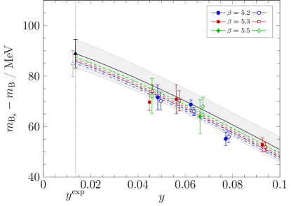
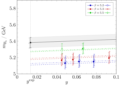
In Fig. 2 we show the continuum and chiral extrapolations of mBssubscript𝑚subscriptBsm_{{\rm B}_{\rm s}} and mBs−mBsubscript𝑚subscriptBssubscript𝑚Bm_{{\rm B}_{\rm s}}-m_{\rm B} at next-to-leading order in 1/mb1subscript𝑚b1/m_{\rm b}. In this and the following Figures, filled symbols and dashed curves represent our HYP1 data set, while open symbols and dash-dotted curves represent our HYP2 data set. For both, equal colours and symbols refer to the same lattice spacing as indicated by equal values of the bare gauge coupling, given by ÎČ=6/g02đ›œ6superscriptsubscript𝑔02\beta=6/g_{0}^{2} in the legend, c.f. Tables 1 and 2. The solid black line is the continuum limit given by the part of the fit function which is independent of the lattice spacing a𝑎a. Accordingly, the difference between the solid and non-solid lines represents the cutoff effect as fitted through a given ansatz.

For the hyperfine splitting, we can perform the chiral and continuum extrapolation using

Δq,ÎŽHF​m​(y,a)subscriptsuperscriptΔHF𝑞𝛿𝑚𝑩𝑎\displaystyle\Delta^{\rm HF}_{q,\delta}m\,(y,a) =[mBq∗−mBq]​[1−cÂŻq​32​g^2​(y​ln⁥y−yexp​ln⁥yexp)+CÂŻq​(y−yexp)]absentdelimited-[]subscript𝑚subscriptsuperscriptB𝑞subscript𝑚subscriptB𝑞delimited-[]1subscript¯𝑐𝑞32superscript^𝑔2𝑩𝑩superscript𝑩expsuperscript𝑩expsubscriptÂŻđ¶đ‘žđ‘Šsuperscript𝑩exp\displaystyle=[m_{{\rm B}^{*}_{q}}-m_{{\rm B}_{q}}]\left[1-\bar{c}_{q}\tfrac{3}{2}\widehat{g}^{2}\left(y\ln{y}-y^{\rm exp}\ln{y^{\rm exp}}\right)+\bar{C}_{q}\left(y-y^{\rm exp}\right)\right]
+DÂŻq,ή​a+DÂŻÂŻq,ή​a2,subscriptÂŻđ·đ‘žđ›żđ‘ŽsubscriptÂŻÂŻđ·đ‘žđ›żsuperscript𝑎2\displaystyle\qquad\qquad\qquad\qquad+\bar{D}_{q,\delta}\,a+\bar{\bar{D}}_{q,\delta}\,a^{2}\;, (2.19)

with the continuum part coinciding, in the case q=d𝑞dq=\rm d, with the expression derived in [45]. Hence, we can probe two ansĂ€tze for the chiral extrapolation by setting cÂŻd=0,1subscript¯𝑐d01\bar{c}_{\rm d}=0,1. Since in principle the O​(a)O𝑎{\rm O}(a) improvement of the hyperfine splitting is not implemented, we have included linear cutoff effects, but also study the scaling behaviour with an O​(a2)Osuperscript𝑎2{\rm O}(a^{2}) ansatz by setting either DÂŻq,ÎŽsubscriptÂŻđ·đ‘žđ›ż\bar{D}_{q,\delta} or DÂŻÂŻq,ÎŽsubscriptÂŻÂŻđ·đ‘žđ›ż\bar{\bar{D}}_{q,\delta} to zero in the equation above. In general, our data is not sensitive enough to clearly separate O​(a)O𝑎{\rm O}(a) scaling from O​(a2)Osuperscript𝑎2{\rm O}(a^{2}) such that individual fits lead to similar results. As additional safety measure we account for a systematic error by increasing the uncertainty of the favoured O​(a)O𝑎{\rm O}(a) extrapolation in order to cover the mean value obtained from the corresponding O​(a2)Osuperscript𝑎2{\rm O}(a^{2}) extrapolation. As will be seen in the following, this only occurs in the case of mBs∗−mBssubscript𝑚subscriptsuperscriptBssubscript𝑚subscriptBsm_{\mathrm{B}^{*}_{\rm s}}-m_{{\rm B}_{\rm s}}.

Since, to our knowledge, no systematic HMÏ‡đœ’\chiPT formulae exist in the literature for the mass splittings mBqr−mBqsubscript𝑚subscriptsuperscriptBr𝑞subscript𝑚subscriptB𝑞m_{{\rm B}^{\rm r}_{q}}-m_{{\rm B}_{q}}, we again employ a simple linear ansatz in mπ2subscriptsuperscript𝑚2𝜋m^{2}_{\pi}:

Δr,qstat​m​(y,a)subscriptsuperscriptΔstatr𝑞𝑚𝑩𝑎\displaystyle\Delta^{\rm stat}_{{\rm r,}q}m\,(y,a) =[mBqr−mBq]stat+Cqstat​(y−yexp)+Eq,ÎŽstat​a2,absentsuperscriptdelimited-[]subscript𝑚subscriptsuperscriptBr𝑞subscript𝑚subscriptB𝑞statsubscriptsuperscriptđ¶stat𝑞𝑩superscript𝑩expsubscriptsuperscript𝐾stat𝑞𝛿superscript𝑎2\displaystyle=[m_{{\rm B}^{\rm r}_{q}}-m_{{\rm B}_{q}}]^{\rm stat}+C^{\rm stat}_{q}(y-y^{\rm exp})+E^{\rm stat}_{q,\delta}a^{2}\;, (2.20)
Δr,q​m​(y,a)subscriptΔr𝑞𝑚𝑩𝑎\displaystyle\Delta_{{\rm r,}q}m\,(y,a) =[mBqr−mBq]+Cqâ€Č​(y−yexp)+Eq,ÎŽâ€Č​a+Eq,ÎŽâ€Čâ€Č​a2.absentdelimited-[]subscript𝑚subscriptsuperscriptBr𝑞subscript𝑚subscriptB𝑞subscriptsuperscriptđ¶â€Č𝑞𝑩superscript𝑩expsubscriptsuperscript𝐾â€Č𝑞𝛿𝑎subscriptsuperscript𝐾â€Čâ€Č𝑞𝛿superscript𝑎2\displaystyle=[m_{{\rm B}^{\rm r}_{q}}-m_{{\rm B}_{q}}]+C^{\prime}_{q}(y-y^{\rm exp})+E^{\prime}_{q,\delta}a+E^{\prime\prime}_{q,\delta}a^{2}\;. (2.21)

For the mass splitting Δr,q​msubscriptΔr𝑞𝑚\Delta_{{\rm r,}q}m\, at next-to-leading order in HQET, one can in fact define

Δr,q1/m​m​(y,a)subscriptsuperscriptΔ1mr𝑞𝑚𝑩𝑎\displaystyle\Delta^{\rm 1/m}_{{\rm r,}q}m\,(y,a) ≡Δr,q​m​(y,a)−Δr,qstat​m​(y,a)absentsubscriptΔr𝑞𝑚𝑩𝑎subscriptsuperscriptΔstatr𝑞𝑚𝑩𝑎\displaystyle\equiv\Delta_{{\rm r,}q}m\,(y,a)-\Delta^{\rm stat}_{{\rm r,}q}m\,(y,a) (2.22)

and take the continuum limit of the leading (static) and next-to-leading order piece (1/m) separately. While for the former eq. (2.20) can be employed, the 1/mb1subscript𝑚b1/m_{\rm b}-correction term has to be extrapolated using ansatz (2.21) with Eq,ÎŽâ€Čâ€Č=0subscriptsuperscript𝐾â€Čâ€Č𝑞𝛿0E^{\prime\prime}_{q,\delta}=0. Both pieces can again be combined after the physical point is reached, leading to an improved signal that is dominated by the static extrapolation. No matter what way is pursued, all extrapolations lead to results that are well compatible within errors.

We perform the full analysis using two static discretizations (HYP1,HYP2) while only one may already suffice. The reason is that the universality of the continuum limit, a property that can be rigorously guaranteed for renormalizable theories, implies that both static discretizations have to lead to equal results in the continuum. At finite lattice spacing the two discretizations have inherently different lattice artifacts, best seen among our observables in Fig. 3. To this end one can either take the two independently in order to show that universality holds or—as we usually do—combine both in one fit in order to stabilise the χ2superscript𝜒2\chi^{2}-minimization. It furthermore serves as a non-trivial check that the whole procedure has been applied correctly and consistently.

3 Results

Using the HQET parameters of Table 1 at zb=13.25subscript𝑧b13.25z_{{\rm b}}=13.25, we obtain for the B-meson mass mB=5.285​(62)subscript𝑚B5.28562m_{\rm B}=5.285(62) GeV by employing eqs. (2.17) and (2.18) with cq=1subscript𝑐𝑞1c_{q}=1 as extrapolation ansatz. Note, however, that the experimental value mB=5.2795subscript𝑚B5.2795m_{\rm B}=5.2795 GeV has been used as input in [15] to fix the b-quark mass. Therefore mBsubscript𝑚Bm_{\rm B} is not a prediction of the theory in our setup, and the number above should be regarded as a consistency check of the approach.

3.1 Ground states
Refer to caption
Refer to caption
Figure 2: Chiral and continuum extrapolation of mBssubscript𝑚subscriptBsm_{{\rm B}_{\rm s}} (left) and mBs−mBsubscript𝑚subscriptBssubscript𝑚Bm_{{\rm B}_{\rm s}}-m_{\rm B} (right) according to (2.18). The open triangle represents the corresponding result for extrapolating the static order data. Here and in the following Figures, filled symbols and dashed curves represent our HYP1 data set, while open symbols and dash-dotted curves represent our HYP2 data set. The solid black line is the continuum limit for the given fit ansatz.

As first quantities beyond mBsubscript𝑚Bm_{\rm B}, we compute the BssubscriptBs{\rm B}_{\rm s}-meson mass and the mass difference mBs−mBsubscript𝑚subscriptBssubscript𝑚Bm_{{\rm B}_{\rm s}}-m_{\rm B}. Their continuum and chiral extrapolations at next-to-leading order in 1/mb1subscript𝑚b1/m_{\rm b} are shown in Fig. 2 and compared to the extrapolated value of the static data at the physical point. The raw data for the mass difference mBs−mBsubscript𝑚subscriptBssubscript𝑚Bm_{{\rm B}_{\rm s}}-m_{\rm B} and the hyperfine splittings is collected in Tables 3 and 4.

From the extrapolation of the form of eqs. (2.17) and (2.18) with cq=0subscript𝑐𝑞0c_{q}=0, we obtain the result:

mBssubscript𝑚subscriptBs\displaystyle m_{{\rm B}_{\rm s}} =5383​(63)​MeV,absent538363MeV\displaystyle=5383(63)\,{\rm MeV}\;, mBs−mBsstatsubscript𝑚subscriptBssuperscriptsubscript𝑚subscriptBsstat\displaystyle m_{{\rm B}_{\rm s}}-m_{{\rm B}_{\rm s}}^{\rm stat} =58​(12)​MeV,absent5812MeV\displaystyle=58(12)\,{\rm MeV}\;, (3.23)

where the error includes statistic and systematic uncertainties (scale setting, HQET parameters), combined in quadrature as explained in Appendix A. Although our result for mBssubscript𝑚subscriptBsm_{{\rm B}_{\rm s}} comes with a much larger error compared to the PDG value, mBs0=5366.77±0.24​MeVsubscript𝑚subscriptsuperscriptB0splus-or-minus5366.770.24MeVm_{\rm B^{0}_{s}}=5366.77\pm 0.24\,{\rm MeV}, the difference between the mean values is only one fourth of our error.

In the combination mBs−mBsubscript𝑚subscriptBssubscript𝑚Bm_{{\rm B}_{\rm s}}-m_{\rm B}, the error is reduced due to correlations among the heavy-light and heavy-strange measurements, although the latter have been performed on a subset of the available ensembles only, as it can be inferred from Table 2.

Our results for the BssubscriptBs{\rm B}_{\rm s}-B mass splitting at O​(1/m)O1𝑚{\rm O}(1/m) and in the static approximation are

mBs−mBsubscript𝑚subscriptBssubscript𝑚B\displaystyle m_{{\rm B}_{\rm s}}-m_{\rm B} =88.9​(5.7)​(2.3)χ​MeV,absent88.95.7subscript2.3𝜒MeV\displaystyle=88.9(5.7)(2.3)_{\chi}\,{\rm MeV}\;, (3.24a)
[mBs−mB]statsuperscriptdelimited-[]subscript𝑚subscriptBssubscript𝑚Bstat\displaystyle[m_{{\rm B}_{\rm s}}-m_{\rm B}]^{{\rm stat}} =85.0​(5.1)​(2.2)χ​MeV,absent85.05.1subscript2.2𝜒MeV\displaystyle=85.0(5.1)(2.2)_{\chi}\,{\rm MeV}\;, (3.24b)

both in good agreement with the PDG value of [1] mBs−mB=87.35​(23)​MeVsubscript𝑚subscriptBssubscript𝑚B87.3523MeVm_{{\rm B}_{\rm s}}-m_{\rm B}=87.35(23)\,{\rm MeV}. Here, the quoted mean and statistical error results from an HMÏ‡đœ’\chiPT extrapolation ansatz that is obtained by appropriately combining eq. (2.18) for the light and strange quark sector. As systematic error due to the chiral extrapolation ansatz we quote its difference to the standard mπ2superscriptsubscript𝑚𝜋2m_{\pi}^{2}-extrapolation.

Refer to caption
Refer to caption
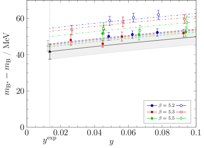
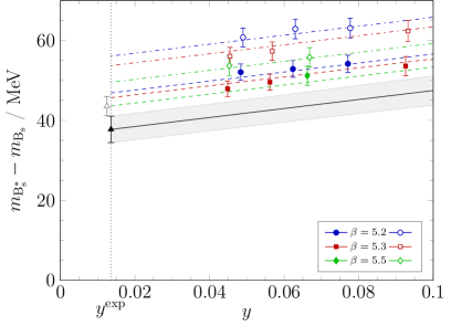
Figure 3: Chiral and continuum extrapolation of the hyperfine spin splitting of the B-meson (left) and of the BssubscriptBs{\rm B}_{\rm s}-meson (right). For mB∗−mBsubscript𝑚superscriptBsubscript𝑚Bm_{\rm B^{*}}-m_{\rm B} we show the extrapolation from ansatz (2.19) with c¯d=1subscript¯𝑐d1\bar{c}_{\rm d}=1 and leading a𝑎a-effects, while for mBs∗−mBssubscript𝑚subscriptsuperscriptBssubscript𝑚subscriptBsm_{\mathrm{B}^{*}_{\rm s}}-m_{{\rm B}_{\rm s}} we have to set c¯s=0subscript¯𝑐s0\bar{c}_{\rm s}=0. In both panels the open triangle at the physical point reflects the corresponding fit result using an a2superscript𝑎2a^{2}-scaling ansatz. Details are given in Table 3.
Δs−d​msubscriptΔsd𝑚\Delta_{\rm s-d}m [MeV] Δs−dstat​msubscriptsuperscriptΔstatsd𝑚\Delta^{\rm stat}_{\rm s-d}m [MeV]
e𝑒e-id y𝑩y HYP1 HYP2 HYP1 HYP2
A4 0.0771(14) 55.2(2.6) 56.0(2.3) 51.9(2.1) 53.1(1.8)
A5 0.0624(13) 68.8(1.8) 66.0(1.6) 62.6(1.8) 63.4(1.7)
B6 0.0484(9) 71.6(4.9) 70.2(3.5) 66.5(3.9) 67.3(3.1)
E5 0.0926(15) 52.8(2.7) 51.9(1.9) 48.8(2.0) 49.2(1.7)
F6 0.0562(9) 70.9(5.7) 70.3(4.0) 66.5(5.2) 64.7(3.9)
F7 0.0449(8) 69.7(3.2) 74.0(2.5) 67.1(3.0) 69.4(2.4)
N6 0.0662(10) 64.0(6.7) 68.0(3.7) 62.8(4.8) 63.3(3.2)
O7 0.0447(7) – 72.2(6.9) – 70.2(5.3)
LO-a2superscript𝑎2a^{2} yexp,a=0superscript𝑩exp𝑎0y^{\rm exp},a=0 91.2(5.8) 87.2(5.2)
NLO-a2superscript𝑎2a^{2} yexp,a=0superscript𝑩exp𝑎0y^{\rm exp},a=0 88.9(5.7) 85.0(5.1)
Table 3: Mass splitting between BssubscriptBs{\rm B}_{\rm s}- and BdsubscriptBd{\rm B}_{\rm d}-meson at static and next-to-leading order HQET.
ΔdHF​msubscriptsuperscriptΔHFd𝑚\Delta^{\rm HF}_{\rm d}\!m [MeV] ΔsHF​msubscriptsuperscriptΔHFs𝑚\Delta^{\rm HF}_{\rm s}\!m [MeV]
e𝑒e-id y𝑩y HYP1 HYP2 HYP1 HYP2
A4 0.0771(14) 52.3(2.1) 62.0(2.4) 54.2(2.2) 63.1(2.5)
A5 0.0624(13) 51.1(2.0) 60.5(2.4) 52.9(2.1) 62.9(2.5)
B6 0.0484(9) 50.1(2.2) 58.7(2.5) 52.1(2.0) 60.8(2.4)
E5 0.0926(15) 51.9(2.1) 59.6(2.4) 53.6(2.4) 62.4(2.7)
F6 0.0562(9) 50.0(2.5) 58.1(2.7) 49.6(2.0) 57.4(2.3)
F7 0.0449(8) 46.1(1.9) 54.1(2.2) 47.9(2.0) 56.1(2.2)
G8 0.0260(5) 48.1(2.9) 53.7(2.6) – –
N5 0.0940(19) 52.6(2.8) 57.7(3.6) – –
N6 0.0662(10) 51.1(3.0) 53.3(2.9) 51.2(2.4) 55.8(2.4)
O7 0.0447(7) 51.7(3.7) 54.4(3.1) – 53.7(2.4)
LO-a2superscript𝑎2a^{2} yexp,a=0superscript𝑩exp𝑎0y^{\rm exp},a=0 45.2(2.9) 43.6(2.4)
LO-a1superscript𝑎1a^{1} yexp,a=0superscript𝑩exp𝑎0y^{\rm exp},a=0 42.0(4.2) 37.8(3.3)
NLO-a2superscript𝑎2a^{2} yexp,a=0superscript𝑩exp𝑎0y^{\rm exp},a=0 44.9(2.9)
NLO-a1superscript𝑎1a^{1} yexp,a=0superscript𝑩exp𝑎0y^{\rm exp},a=0 41.7(4.2)
Table 4: Hyperfine splittings in the light- and strange-quark sector.

For the hyperfine spin splittings, we obtain

mB∗−mBsubscript𝑚superscriptBsubscript𝑚B\displaystyle m_{\rm B^{*}}-m_{\rm B} =41.7​(4.2)​(3.2)a​(0.3)χ​MeV,absent41.74.2subscript3.2𝑎subscript0.3𝜒MeV\displaystyle=41.7(4.2)(3.2)_{a}(0.3)_{\chi}\,{\rm MeV}\;, (3.25a)
mBs∗−mBssubscript𝑚subscriptsuperscriptBssubscript𝑚subscriptBs\displaystyle m_{\mathrm{B}^{*}_{\rm s}}-m_{{\rm B}_{\rm s}} =37.8​(3.3)​(5.8)a​MeV,absent37.83.3subscript5.8𝑎MeV\displaystyle=37.8(3.3)(5.8)_{a}\,{\rm MeV}\;, (3.25b)

where we quote the mean value obtained with c¯d=1subscript¯𝑐d1\bar{c}_{\rm d}=1 for the B-meson case and add the difference w.r.t. the result obtained from the ansatz with c¯d=0subscript¯𝑐d0\bar{c}_{\rm d}=0 as a systematic error estimate for the chiral extrapolation. As mentioned earlier, we also account here for a systematic error between linear and quadratic continuum extrapolations. The O​(a)O𝑎{\rm O}(a) extrapolations are shown for both the B and the BssubscriptBs{\rm B}_{\rm s} system in Fig. 3. The filled/empty symbols at the physical point are the results using either an O​(a)O𝑎{\rm O}(a), or an O​(a2)Osuperscript𝑎2{\rm O}(a^{2}) term in the continuum extrapolation.

Our result for the hyperfine splitting for the B-system is in good agreement with the experimental value mB∗−mB=45.78​(35)​MeVsubscript𝑚superscriptBsubscript𝑚B45.7835MeVm_{\rm B^{*}}-m_{\rm B}=45.78(35)\,{\rm MeV} [1], whereas the BssubscriptBs{\rm B}_{\rm s} hyperfine splitting differs noticeably from the experimental value mBs∗−mBs=48.7​+2.3−2.1​MeVsubscript𝑚subscriptsuperscriptBssubscript𝑚subscriptBs48.7FRACOP2.32.1MeVm_{\mathrm{B}^{*}_{\rm s}}-m_{{\rm B}_{\rm s}}=48.7{+2.3\atop-2.1}\,{\rm MeV}. Our results are smaller than the experimental value and than our result for the hyperfine splitting of the B (the opposite of the situation for the experimental values). Since the hyperfine splitting came out far too small in the quenched approximation [39], this is suggestive of a residual quenching effect from the quenching of the strange quark in our Nf=2subscript𝑁f2N_{\rm f}=2 simulations. Moreover, Fig. 3 indicates larger cutoff effects in the case of the hyperfine splitting for the BssubscriptBs{\rm B}_{\rm s}.

3.2 Excited states

Δr,d​msubscriptΔrd𝑚\Delta_{{\rm r,}\rm d}m\, [GeV] Δr,dstat​msubscriptsuperscriptΔstatrd𝑚\Delta^{\rm stat}_{{\rm r,}\rm d}m\, [GeV]
e𝑒e-id y𝑩y HYP1 HYP2 HYP1 HYP2
A4 0.0771(14) 0.692(37) 0.703(33) 0.619(27) 0.625(25)
A5 0.0624(13) 0.736(18) 0.738(17) 0.655(16) 0.664(15)
B6 0.0484(9) 0.622(66) 0.665(57) 0.552(56) 0.592(52)
E5 0.0926(15) 0.753(27) 0.758(25) 0.676(24) 0.682(23)
F6 0.0562(9) 0.719(57) 0.721(54) 0.658(52) 0.654(47)
F7 0.0449(8) 0.760(32) 0.756(26) 0.678(32) 0.676(30)
G8 0.0260(5) 0.67(11) 0.70(9) 0.63(11) 0.65(9)
N5 0.0940(19) 0.83(11) 0.71(14) 0.697(35) 0.709(31)
N6 0.0662(10) 0.78(9) 0.76(8) 0.634(72) 0.668(58)
O7 0.0447(7) 0.71(12) 0.71(8) 0.64(10) 0.63(8)
LO-a2superscript𝑎2a^{2} yexp,a=0superscript𝑩exp𝑎0y^{\rm exp},a=0 0.787(71) 0.701(65)
LO-a1superscript𝑎1a^{1} yexp,a=0superscript𝑩exp𝑎0y^{\rm exp},a=0 0.84(12)
Table 5: Mass gaps between the excited state BdrsubscriptsuperscriptBrd{\rm B}^{\rm r}_{\rm d}- and the BdsubscriptBd{\rm B}_{\rm d}-meson at static and next-to-leading order HQET.
Δr,s​msubscriptΔrs𝑚\Delta_{{\rm r,}\rm s}m\, [GeV] Δr,sstat​msubscriptsuperscriptΔstatrs𝑚\Delta^{\rm stat}_{{\rm r,}\rm s}m\, [GeV]
e𝑒e-id y𝑩y HYP1 HYP2 HYP1 HYP2
A4 0.0771(14) 0.774(45) 0.748(34) 0.640(23) 0.650(22)
A5 0.0624(13) 0.760(15) 0.753(15) 0.670(11) 0.677(11)
B6 0.0484(9) 0.719(49) 0.704(35) 0.641(22) 0.641(21)
E5 0.0926(15) 0.791(66) 0.676(44) 0.609(29) 0.624(25)
F6 0.0562(9) 0.689(30) 0.722(24) 0.643(18) 0.642(17)
F7 0.0449(8) 0.665(24) 0.660(19) 0.593(15) 0.601(14)
N6 0.0662(10) 0.698(49) 0.718(36) 0.621(38) 0.643(32)
O7 0.0447(7) – 0.736(38) – 0.669(29)
LO-a2superscript𝑎2a^{2} yexp,a=0superscript𝑩exp𝑎0y^{\rm exp},a=0 0.570(47) 0.547(34)
LO-a1superscript𝑎1a^{1} yexp,a=0superscript𝑩exp𝑎0y^{\rm exp},a=0 0.519(74)
Table 6: Mass gaps between the excited state BsrsubscriptsuperscriptBrs{\rm B}^{\rm r}_{\rm s}- and the BssubscriptBs{\rm B}_{\rm s}-meson at static and next-to-leading order HQET.
Δr,d1/m​msubscriptsuperscriptΔ1mrd𝑚\Delta^{\rm 1/m}_{{\rm r,}\rm d}m\, [MeV] Δr,s1/m​msubscriptsuperscriptΔ1mrs𝑚\Delta^{\rm 1/m}_{{\rm r,}\rm s}m\, [MeV]
e𝑒e-id y𝑩y HYP1 HYP2 HYP1 HYP2
A4 0.0771(14) 73(27) 78(21) 133(38) 98(26)
A5 0.0624(13) 71(11) 75( 8) 90(11) 76( 9)
B6 0.0484(9) 70(31) 73(20) 78(45) 64(28)
E5 0.0926(15) 77(17) 75( 9) 182(71) 52(40)
F6 0.0562(9) 61(31) 68(21) 47(24) 80(17)
F7 0.0449(8) 82(18) 80(11) 71(19) 59(15)
G8 0.0260(5) 36(26) 54(15) – –
N5 0.0940(19) 132(110) 6(95) – –
N6 0.0662(10) 149(59) 94(31) 77(31) 76(18)
O7 0.0447(7) 75(25) 84(17) – 67(26)
LO-a1superscript𝑎1a^{1} yexp,a=0superscript𝑩exp𝑎0y^{\rm exp},a=0 0.090(40) 0.019(46)
Table 7: Subleading HQET contributions to the mass gaps between excited and ground states.
Refer to caption
Refer to caption
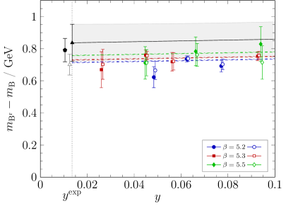
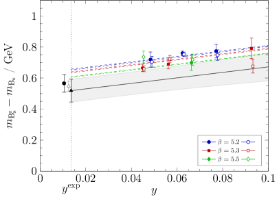
Figure 4: Chiral and continuum extrapolation of mBr−mBsubscript𝑚superscriptBrsubscript𝑚Bm_{{\rm B}^{\rm r}}-m_{\rm B} (left) and mBsr−mBssubscript𝑚subscriptsuperscriptBrssubscript𝑚subscriptBsm_{{\rm B}^{\rm r}_{\rm s}}-m_{{\rm B}_{\rm s}} (right). Both represent an extrapolation with ansatz (2.21) and Eq,ÎŽâ€Čâ€Č=0subscriptsuperscript𝐾â€Čâ€Č𝑞𝛿0E^{\prime\prime}_{q,\delta}=0 for HQET to order 1/mb1subscript𝑚b1/m_{\rm b}. The open triangle represents the corresponding result for extrapolating the static order data. For details see Tables 5 and 6. We also add the continuum point (filled black pentagon) corresponding to the combination given in eq. (3.26).
Refer to caption
Refer to caption
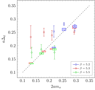
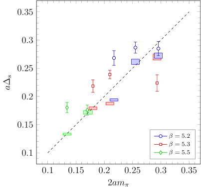
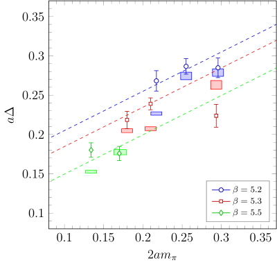
Figure 5: The measured gap mBqr−mBqsubscript𝑚subscriptsuperscriptBr𝑞subscript𝑚subscriptB𝑞m_{{\rm B}^{\rm r}_{q}}-m_{{\rm B}_{q}} vs. 2​mπ2subscript𝑚𝜋2m_{\pi} for the excited states BqrsubscriptsuperscriptBr𝑞{\rm B}^{\rm r}_{q} with q=d𝑞dq={\rm d} (left) and q=s𝑞sq={\rm s} (right) on each individual CLS ensemble and with HYP2 discretization of the static quark. The boxes are an estimate of the expected gap for a two-hadron state Bq∗​(−p)+π​(p)subscriptsuperscriptB𝑞𝑝𝜋𝑝\mathrm{B}^{*}_{q}(-p)+\pi(p) with one unit of lattice momentum p=|đ©|=2​π/Lđ‘đ©2𝜋𝐿p=|{\bf p}|=2\pi/L. The lower edge of the boxes corresponds to ΔqHF​m+mπ2+(2​π/L)2subscriptsuperscriptΔHF𝑞𝑚superscriptsubscript𝑚𝜋2superscript2𝜋𝐿2\Delta^{\rm HF}_{q}\!m+\sqrt{m_{\pi}^{2}+(2\pi/L)^{2}} and the upper edge includes an additional contribution đ©2/(2​mBq∗)superscriptđ©22subscript𝑚subscriptsuperscriptB𝑞{\bf p}^{2}/(2m_{{\rm B}^{*}_{q}}) as a naive estimate for the kinetic energy of the Bq∗subscriptsuperscriptB𝑞\mathrm{B}^{*}_{q}. The dotted line is Δ=2​mπΔ2subscript𝑚𝜋\Delta=2m_{\pi} corresponding to a three-hadron state Bq+π+πsubscriptB𝑞𝜋𝜋{\rm B}_{q}+\pi+\pi.
Refer to caption
Figure 6: The same data points as in the right panel of Fig. 5 for the measured BsrsubscriptsuperscriptBrs{\rm B}^{\rm r}_{\rm s} mass gaps, together with estimates of the energy gap for a two-hadron state B∗​(−p)+K​(p)superscriptB𝑝K𝑝\mathrm{B}^{*}(-p)+\mathrm{K}(p) (boxes) and a three-hadron state Bd+K+πsubscriptBdK𝜋{\rm B}_{\rm d}+\mathrm{K}+\pi (dashed lines).

For the mass splittings between the ground state BqsubscriptB𝑞{\rm B}_{q} and the first excited state, denoted here by BrsuperscriptBr{\rm B}^{\rm r} and BsrsubscriptsuperscriptBrs{\rm B}^{\rm r}_{\rm s}, we obtain

mBr−mBsubscript𝑚superscriptBrsubscript𝑚B\displaystyle m_{{\rm B}^{\rm r}}-m_{\rm B} =791​(73)​MeV,absent79173MeV\displaystyle=791(73)\,{\rm MeV}\;, [mBr−mB]statsuperscriptdelimited-[]subscript𝑚superscriptBrsubscript𝑚Bstat\displaystyle[m_{{\rm B}^{\rm r}}-m_{\rm B}]^{{\rm stat}} =701​(65)​MeV,absent70165MeV\displaystyle=701(65)\,{\rm MeV}\;, (3.26a)
mBsr−mBssubscript𝑚subscriptsuperscriptBrssubscript𝑚subscriptBs\displaystyle m_{{\rm B}^{\rm r}_{\rm s}}-m_{{\rm B}_{\rm s}} =566​(57)​MeV,absent56657MeV\displaystyle=566(57)\,{\rm MeV}\;, [mBsr−mBs]statsuperscriptdelimited-[]subscript𝑚subscriptsuperscriptBrssubscript𝑚subscriptBsstat\displaystyle[m_{{\rm B}^{\rm r}_{\rm s}}-m_{{\rm B}_{\rm s}}]^{{\rm stat}} =547​(34)​MeV.absent54734MeV\displaystyle=547(34)\,{\rm MeV}\;. (3.26b)

after adding the individually extrapolated results for [mBqr−mBq]statsuperscriptdelimited-[]subscript𝑚subscriptsuperscriptBr𝑞subscript𝑚subscriptB𝑞stat[m_{{\rm B}^{\rm r}_{q}}-m_{{\rm B}_{q}}]^{\rm stat} and [mBqr−mBq]1/msuperscriptdelimited-[]subscript𝑚subscriptsuperscriptBr𝑞subscript𝑚subscriptB𝑞1m[m_{{\rm B}^{\rm r}_{q}}-m_{{\rm B}_{q}}]^{\rm 1/m}. In Fig. 4 these values are shown (as pentagons, slightly shifted at the physical point) for comparison with an extrapolation according to eq. (2.21). The raw data is collected in Tables 5, 6, and 7.

We conclude this Section by remarking that for the excited states the interpretation of our results in terms of mass differences of physical one-meson states, e.g. “radial excitations”, is not straight forward. Although our values for these mass gaps are larger than what a multi-hadron state made of, e.g., a B(s)(∗)subscriptsuperscriptabsents{}^{(*)}_{(\rm s)}-meson and a small number (≀2absent2\leq 2) of physical pions would produce, we cannot unambiguously conclude that our BqrsubscriptsuperscriptBr𝑞{\rm B}^{\rm r}_{q} states actually correspond to radial excitations of the ground-state BqsubscriptB𝑞{\rm B}_{q}-mesons. In a rigorous approach, states above multi-hadron thresholds need to be treated as resonances in order to obtain precise values for their masses and widths, and to associate them with the states observable in experiments.

Since our lattice study is unquenched, the excited states can also be multi-particle states involving additional pions, beside the desired one-particle state. While it has been argued that the overlap of single-hadron interpolating operators to multi-hadron states is small [46, 47], the two-hadron states may have a weaker volume suppression [48]. Moreover, a chiral extrapolation linear in mπ2subscriptsuperscript𝑚2𝜋m^{2}_{\pi} might not be adequate for a multi-hadron state, and a different extrapolation ansatz for these states, e.g. linear in mπsubscript𝑚𝜋m_{\pi}, might also yield somewhat smaller mass gaps.

In continuum (and infinite-volume) physics, any excited BqsubscriptB𝑞{\rm B}_{q}-meson state, BqxsubscriptsuperscriptBx𝑞{\rm B}^{\rm x}_{q}, which strongly decays into an ℓℓ\ell-wave Bq+πsubscriptB𝑞𝜋{\rm B}_{q}+\pi state, i.e. a resonance in the ℓℓ\ell-wave Bq+πsubscriptB𝑞𝜋{\rm B}_{q}+\pi scattering channel, implies that the corresponding two-hadron state Bqx+πsubscriptsuperscriptBx𝑞𝜋{\rm B}^{\rm x}_{q}+\pi with relative angular momentum ℓℓ\ell has the correct quantum numbers to couple to our interpolating operators used for the BqsubscriptB𝑞{\rm B}_{q}. For the q=d𝑞dq={\rm d} sector, the set of possible two-hadron excited states includes

  • ‱

    B∗+πsuperscriptB∗𝜋{\rm B}^{\ast}+\pi in P-wave which would have a non-interacting two-hadron energy gap of Δ≳181​MeVgreater-than-or-equivalent-toΔ181MeV\Delta\gtrsim 181\,{\rm MeV},

  • ‱

    Bâ€Č⁣∗+πsuperscriptBâ€Č∗𝜋{\rm B}^{\prime\ast}+\pi in P-wave, where Bâ€Č⁣∗superscriptBâ€Č∗{\rm B}^{\prime\ast} is a radial excitation (JP=1−superscriptđœđ‘ƒsuperscript1J^{P}=1^{-}),

  • ‱

    B0∗+πsuperscriptsubscriptB0∗𝜋{\rm B}_{0}^{\ast}+\pi in S-wave, where B0∗superscriptsubscriptB0∗{\rm B}_{0}^{\ast} is an orbital excitation (JP=0+superscriptđœđ‘ƒsuperscript0J^{P}=0^{+}),

  • ‱

    B2∗+πsuperscriptsubscriptB2∗𝜋{\rm B}_{2}^{\ast}+\pi in D-wave, where B2∗superscriptsubscriptB2∗{\rm B}_{2}^{\ast} is an orbital excitation (JP=2+superscriptđœđ‘ƒsuperscript2J^{P}=2^{+}), like the observed B2∗​(5747)0superscriptsubscriptB2∗superscript57470{\rm B}_{2}^{\ast}(5747)^{0} state which would lead to a non-interacting two-hadron energy gap of Δ≳598​MeVgreater-than-or-equivalent-toΔ598MeV\Delta\gtrsim 598\,{\rm MeV}.

On a finite lattice, the energies of states with non-zero relative angular momentum are lifted due to the minimal momentum of |đ©|=2​π/Lđ©2𝜋𝐿|{\bf p}|=2\pi/L. Since the s-quark is quenched in our study, we cannot have excited states in the B sector with an s-quark from the sea, like Bs∗+KsubscriptsuperscriptBsK\mathrm{B}^{*}_{\rm s}+\textrm{K}. On the other hand, in the BssubscriptBs{\rm B}_{\rm s} sector there are two flavour combinations for each of the corresponding excited state of the B sector, e.g. Bs∗+πsubscriptsuperscriptBs𝜋\mathrm{B}^{*}_{\rm s}+\pi and B∗+KsuperscriptBK\mathrm{B}^{*}+\textrm{K} (corresponding to B∗+πsuperscriptB𝜋\mathrm{B}^{*}+\pi).

In Figs. 5 and 6 we show our data points on the various ensembles together with an estimate for the gaps of some two-hadron states. The comparison indicates that some of the two-hadron states can be close in energy to the excited states we measured. Depending on the pion mass on a given ensemble, the energy gaps determined according to eqs. (2.16) may in fact be the energy splitting to the lowest lying Bx+πsuperscriptBx𝜋{\rm B}^{\rm x}+\pi state, if this is lighter than the radial excitations Bqâ€ČsubscriptsuperscriptBâ€Č𝑞\mathrm{B}^{\prime}_{q}.

Below three- or more-hadron thresholds, the infinite volume scattering matrix (up to corrections which vanish exponentially in the spatial lattice extent) may be inferred from the finite volume energy spectrum [49, 50, 51, 52, 53]. In practice this requires the construction of correlation matrices which contain two-hadron as well as single hadron operators. To date, this procedure has been carried out successfully in some simple systems such as Ï€âˆ’Ï€đœ‹đœ‹\pi\!-\!\pi and π−limit-from𝜋\pi-K scattering, and the energy dependence of the scattering phase shift has been determined with a sufficient resolution to clearly discern resonant behaviour (see e.g. [54] for a recent review). Without performing such a dedicated study, we are not able to conclusively determine the nature of the excited state we observe.

Source mBssubscript𝑚subscriptBsm_{{\rm B}_{\rm s}} mB∗−mBsubscript𝑚superscriptBsubscript𝑚Bm_{\rm B^{*}}-m_{\rm B} mBs∗−mBssubscript𝑚subscriptsuperscriptBssubscript𝑚subscriptBsm_{\mathrm{B}^{*}_{\rm s}}-m_{{\rm B}_{\rm s}} mBs−mBsubscript𝑚subscriptBssubscript𝑚Bm_{{\rm B}_{\rm s}}-m_{\rm B} mBr−mBsubscript𝑚superscriptBrsubscript𝑚Bm_{{\rm B}^{\rm r}}-m_{\rm B} mBsr−mBssubscript𝑚subscriptsuperscriptBrssubscript𝑚subscriptBsm_{{\rm B}^{\rm r}_{\rm s}}-m_{{\rm B}_{\rm s}}
↓↓\downarrow 5383​(63)5383635383(63) 41.7​(4.2)41.74.241.7(4.2) 37.8​(3.3)37.83.337.8(3.3) 88.9​(5.7)88.95.788.9(5.7) 791​(73)79173791(73) 566​(57)56657566(57)
A4 20.46 % 22.52 % 23.51 % 12.48 % 29.79 % 29.93 %
A5 20.30 % 21.32 % 21.81 % 23.14 % 26.67 % 25.78 %
B6 20.03 % 21.50 % 20.39 % 20.23 % 21.04 % 20.06 %
E5 20.28 % 20.40 % 21.80 % 20.46 % 24.72 % 21.51 %
F6 20.10 % 20.34 % 20.45 % 28.62 % 25.07 % 26.72 %
F7 20.21 % 20.82 % 21.50 % 34.56 % 17.87 % 23.42 %
G8 20.53 % 25.25 % 20.00 % 20.05 % 26.46 % 20.03 %
N5 21.90 % 28.04 % 20.45 % 20.01 % 27.94 % 20.05 %
N6 25.97 % 21.33 % 29.18 % 31.56 % 14.60 % 27.70 %
O7 24.50 % 26.34 % 13.49 % 28.05 % 25.32 % 14.42 %
Ï‰đœ”\omega 62.84 % 31.75 % 46.61 % 20.04 % 20.09 % 20.05 %
ZAsubscript𝑍AZ_{\rm A} 21.13 % 20.27 % 20.63 % 20.75 % 20.40 % 20.19 %
Table 8: Distributions of relative squared errors, σi2/∑jσj2superscriptsubscript𝜎𝑖2subscript𝑗superscriptsubscript𝜎𝑗2\sigma_{i}^{2}/\sum_{j}\sigma_{j}^{2} among different sources i𝑖i for the mean values given in (3.23)-(3.26). In the second row we repeat them in MeV for the reader’s convenience, including only the statistical error of the mean. Remaining relative errors enter through the scale setting procedure only.

4 Conclusions

In this paper, we have presented results for the B-meson spectrum obtained in the framework of lattice HQET expanded to O​(1/mb)O1subscript𝑚b{\rm O}(1/m_{\rm b}). Within this approach the existence of a continuum limit is guaranteed, as numerically tested with high accuracy in previous studies [55, 56]. In contrast to the HQET expansion in continuum perturbation theory, our approach is manifestly non-perturbative in the strong coupling. We perform the continuum extrapolation from lattice resolutions in the range 0.08–0.05 fm. Pion masses, in our setup with Nf=2subscript𝑁f2N_{\rm f}=2 degenerate flavours, reach down to values of about 190 MeV. The accuracy is at the 10% level, for the different splittings presented (e.g., hyperfine and BdsubscriptBd{\rm B}_{\rm d}–BssubscriptBs{\rm B}_{\rm s} splittings), and we always find consistency within two standard deviations with values from the PDG, whenever a comparison is possible.

Hyperfine splittings probe higher-order terms in HQET and the reported results represent an important check on the validity and the reliability of the asymptotic HQET expansion, truncated at NLO, at the b-quark mass scale. Compared to previous quenched results, we observe a significant shift for the hyperfine splitting in the B-meson sector, which now agrees with the experimental determination. In our Nf=2subscript𝑁f2N_{\rm f}=2 simulations, the hyperfine splitting in the BssubscriptBs{\rm B}_{\rm s} sector appears to suffer from a residual quenching effect, which is in line with what was seen for Nf=0subscript𝑁f0N_{\rm f}=0. In order to ascertain that the quenching of the strange quark is indeed the root cause of the reduced BssubscriptBs{\rm B}_{\rm s} hyperfine splitting seen here, we plan to extend our computations to simulations of the Nf=2+1subscript𝑁f21N_{\rm f}=2+1 theory [57].

A dominant source of uncertainty in our results is represented by cutoff effects (see Tab. 8). This does not come unexpected since we have not implemented O​(a)O𝑎{\rm O}(a) improvement at O​(1/mb)O1subscript𝑚b{\rm O}(1/m_{\rm b}). While implementing a fully non-perturbative improvement programme at this order is probably too difficult, one may consider perturbative (tree level or one-loop) improvement for future applications.

We also determined the mass gaps for excited states in both the B and the BssubscriptBs{\rm B}_{\rm s} sectors. The results are consistent with a radial splitting, e.g. as computed for the BcsubscriptBc{\rm B}_{\rm c} system in [9], but these excited states might also be two- or multi-hadron states.

Knowledge of the mass splittings is relevant for the computation of hadronic parameters within the sum-rules approach and when comparing results from the lattice to sum-rules estimates. The mass gaps of excited states are also an important information for the computation of form-factors on the lattice, for example for the B→π​ℓ​Μ→B𝜋ℓ𝜈{\rm B}\to\pi\ell\nu and the Bs→K​ℓ​Μ→subscriptBsKℓ𝜈{\rm B}_{\rm s}\to{\rm K}\ell\nu decays, as currently endeavored by the ALPHA Collaboration [14, 12], and in general in the spectral analysis of two- and three-point functions.


Acknowledgements. We like to thank R. Sommer for many helpful discussions and contributions to the study presented here, and we thank our colleagues in the CLS effort for the joint production and use of gauge configurations. We acknowledge partial support by the SFB/TR 9, by grant HE 4517/2-1 (P.F. and J.H.) and HE 4517/3-1 (J.H.) of the Deutsche Forschungsgemeinschaft, by the European Community through EU Contract MRTN-CT-2006-035482, “FLAVIAnet”, by the Spanish Minister of Education and Science projects RyC-2011-08557 and by the Danish National Research Foundation under the grant n. DNRF:90 (M.D.M.). P.F. acknowledges financial support from the Spanish MINECO under grants FPA2012-31880 and SEV-2012-0249 (“Centro de Excelencia Severo Ochoa” Programme). N.G is supported by the Leverhulme trust, research grant RPG-2014-118.

We gratefully acknowledge the computer resources granted by the John von Neumann Institute for Computing (NIC) and provided on the supercomputer JUROPA at JĂŒlich Supercomputing Centre (JSC) and by the Gauss Centre for Supercomputing (GCS) through the NIC on the GCS share of the supercomputer JUQUEEN at JSC, with funding by the German Federal Ministry of Education and Research (BMBF) and the German State Ministries for Research of Baden-WĂŒrttemberg (MWK), Bayern (StMWFK) and Nordrhein-Westfalen (MIWF), as well as within the Distributed European Computing Initiative by the PRACE-2IP, with funding from the European Community’s Seventh Framework Programme (FP7/2007-2013) under grant agreement RI-283493, by the Grand Équipement National de Calcul Intensif at CINES in Montpellier under the allocation 2012-056808, by the HLRN in Berlin, and by NIC at DESY, Zeuthen.

Appendix A Determination of the statistical error in the presence of autocorrelations

In order to compute the statistical error in the presence of both correlations between the different observables and of autocorrelations along the HMC trajectories by which our ensembles were generated, we employ the methods of [58, 59, 60, 61], which we briefly outline below.

The starting point is the computation of the “primary” observables Cαisubscriptsuperscriptđ¶đ‘–đ›ŒC^{i}_{\alpha}, where i𝑖i labels the Nmeassubscript𝑁measN_{\rm meas} gauge configurations, and Î±đ›Œ\alpha is an aggregate label for the different correlators measured (stat, spin, kin), the Euclidean time separation t𝑡t between the source and sink, and the different smearing levels employed at source and sink. The gauge average C¯αsubscriptÂŻđ¶đ›Œ\overline{C}_{\alpha} and the variance σCα2subscriptsuperscript𝜎2subscriptđ¶đ›Œ\sigma^{2}_{C_{\alpha}} are computed as usual. To estimate the true statistical error σC¯αsubscript𝜎subscriptÂŻđ¶đ›Œ\sigma_{\overline{C}_{\alpha}} of the gauge average, we also require the integrated autocorrelation time τCαintsubscriptsuperscript𝜏intsubscriptđ¶đ›Œ\tau^{\rm int}_{C_{\alpha}}, which is computed from the autocorrelation function

Γα​ÎČ(1)≡ΓCα​CÎČ​(τ)=limK→∞1K​∑i=1K(Cαi+τ−C¯α)​(CÎČi−CÂŻÎČ),subscriptsuperscriptΓ1đ›Œđ›œsubscriptΓsubscriptđ¶đ›Œsubscriptđ¶đ›œđœsubscriptâ†’đŸ1đŸsuperscriptsubscript𝑖1đŸsuperscriptsubscriptđ¶đ›Œđ‘–đœsubscriptÂŻđ¶đ›Œsuperscriptsubscriptđ¶đ›œđ‘–subscriptÂŻđ¶đ›œ\Gamma^{(1)}_{\alpha\beta}\equiv\Gamma_{C_{\alpha}C_{\beta}}(\tau)=\lim_{K\to\infty}\frac{1}{K}\sum_{i=1}^{K}\left(C_{\alpha}^{i+\tau}-\overline{C}_{\alpha}\right)\left(C_{\beta}^{i}-\overline{C}_{\beta}\right)\,, (A.27)

where Ï„đœ\tau is the separation in simulation time along the Markov chain. In order to take into account the long-time tail of ΓΓ\Gamma, the conservative estimate [59]

τCαint=12+1Γα​α(1)​(0)​(∑τ=1W−1Γα​α(1)​(τ)+τexp​Γα​α(1)​(W))subscriptsuperscript𝜏intsubscriptđ¶đ›Œ121subscriptsuperscriptΓ1đ›Œđ›Œ0superscriptsubscript𝜏1𝑊1subscriptsuperscriptΓ1đ›Œđ›Œđœsuperscript𝜏expsubscriptsuperscriptΓ1đ›Œđ›Œđ‘Š\tau^{\rm int}_{C_{\alpha}}=\frac{1}{2}+\frac{1}{\Gamma^{(1)}_{\alpha\alpha}(0)}\left(\sum_{\tau=1}^{W-1}\Gamma^{(1)}_{\alpha\alpha}(\tau)+\tau^{\rm exp}\Gamma^{(1)}_{\alpha\alpha}(W)\right) (A.28)

is used, where τexpsuperscript𝜏exp\tau^{\rm exp} is an estimate of the exponential autocorrelation time of the Markov chain. The values used in our analysis are listed in Table 2. The window size W𝑊W is automatically chosen as the point τ=W𝜏𝑊\tau=W where Γα​α​(τ)subscriptÎ“đ›Œđ›Œđœ\Gamma_{\alpha\alpha}(\tau) comes close to zero within about 1.5 of its estimated error. The true statistical error is then given by

σC¯α2=2​τCαint​σCα2Nmeas.subscriptsuperscript𝜎2subscriptÂŻđ¶đ›Œ2subscriptsuperscript𝜏intsubscriptđ¶đ›Œsubscriptsuperscript𝜎2subscriptđ¶đ›Œsubscript𝑁meas\sigma^{2}_{\overline{C}_{\alpha}}=2\tau^{\rm int}_{C_{\alpha}}\frac{\sigma^{2}_{C_{\alpha}}}{N_{\rm meas}}\,. (A.29)

For derived observables Dαâ€Čsubscriptđ·superscriptđ›Œâ€ČD_{\alpha^{\prime}}, which are functions of gauge averages of the primary observables C¯αsubscriptÂŻđ¶đ›Œ\overline{C}_{\alpha}, and in our case include the generalized eigenvalues and eigenvectors as well as the energies derived from them, we compute the derivatives

Jαâ€Čâ€‹Î±â‰Ąâˆ‚Dαâ€Č∂C¯αsubscriptđœsuperscriptđ›Œâ€Čđ›Œsubscriptđ·superscriptđ›Œâ€ČsubscriptÂŻđ¶đ›ŒJ_{\alpha^{\prime}\alpha}\equiv\frac{\partial D_{\alpha^{\prime}}}{\partial\overline{C}_{\alpha}} (A.30)

and the autocorrelation function [59]

Γαâ€Č​ÎČâ€Č(2)​(τ)â‰Ąâˆ‘Î±,ÎČJαâ€Č​α​Γα​ÎČ(1)​(τ)​JÎČâ€Č​ÎČ.subscriptsuperscriptΓ2superscriptđ›Œâ€Čsuperscriptđ›œâ€Č𝜏subscriptđ›Œđ›œsubscriptđœsuperscriptđ›Œâ€Čđ›ŒsubscriptsuperscriptΓ1đ›Œđ›œđœsubscriptđœsuperscriptđ›œâ€Čđ›œ\Gamma^{(2)}_{\alpha^{\prime}\beta^{\prime}}(\tau)\equiv\sum_{\alpha,\beta}J_{\alpha^{\prime}\alpha}\Gamma^{(1)}_{\alpha\beta}(\tau)J_{\beta^{\prime}\beta}\,. (A.31)

The variance of the derived observable Dαâ€Čsubscriptđ·superscriptđ›Œâ€ČD_{\alpha^{\prime}} is then given by

σDαâ€Č2=Γαâ€Č​αâ€Č(2)​(0)subscriptsuperscript𝜎2subscriptđ·superscriptđ›Œâ€ČsubscriptsuperscriptΓ2superscriptđ›Œâ€Čsuperscriptđ›Œâ€Č0\sigma^{2}_{D_{\alpha^{\prime}}}=\Gamma^{(2)}_{\alpha^{\prime}\alpha^{\prime}}(0) (A.32)

and its statistical error by

σD¯αâ€Č2=2​τDαâ€Čint​σDαâ€Č2Nmeas,subscriptsuperscript𝜎2superscriptsubscriptÂŻđ·đ›Œâ€Č2subscriptsuperscript𝜏intsuperscriptsubscriptđ·đ›Œâ€Čsubscriptsuperscript𝜎2superscriptsubscriptđ·đ›Œâ€Čsubscript𝑁meas\sigma^{2}_{\overline{D}_{\alpha}^{\prime}}=2\tau^{\rm int}_{D_{\alpha}^{\prime}}\frac{\sigma^{2}_{D_{\alpha}^{\prime}}}{N_{\rm meas}}\,, (A.33)

where the integrated autocorrelation time τDαâ€Čintsubscriptsuperscript𝜏intsuperscriptsubscriptđ·đ›Œâ€Č\tau^{\rm int}_{D_{\alpha}^{\prime}} is again estimated using (A.28), with Γ(2)superscriptΓ2\Gamma^{(2)} substituted for Γ(1)superscriptΓ1\Gamma^{(1)}.

Since the extraction of plateau values from a weighted fit requires knowledge of the errors of the individual points, in principle this procedure should be iterated, with the plateau averages as secondary derived observables of the derived observables. However, the integrated autocorrelation times for the effective energies in the plateau region do not markedly differ. Therefor, it is sufficient to employ their variances (as estimated using e.g. a Jackknife procedure for error propagation) to weight the fit, treating only the fitted values as derived observables. This simplified procedure has been adopted here.

In order to extract the final answer in physical units, the plateau values must be combined with each other and with the HQET parameters and lattice spacing, propagating the errors on each of those to the final result, where the HQET parameters are statistically independent of the large-volume observables; similarly, in extrapolating to the chiral and continuum limits, the results obtained from different ensembles are statistically independent, and their contribution to the error of the final result f𝑓f can thus be added in quadrature:

σf2=∑eσf2​(e)+∑i,j∂f∂Yi​CYi​Yj​∂f∂Yj,subscriptsuperscript𝜎2𝑓subscript𝑒subscriptsuperscript𝜎2𝑓𝑒subscript𝑖𝑗𝑓subscript𝑌𝑖subscriptđ¶subscript𝑌𝑖subscript𝑌𝑗𝑓subscript𝑌𝑗\sigma^{2}_{f}=\sum_{e}\sigma^{2}_{f}(e)+\sum_{i,j}\frac{\partial f}{\partial Y_{i}}C_{Y_{i}Y_{j}}\frac{\partial f}{\partial Y_{j}}\,, (A.34)

where the Yisubscript𝑌𝑖Y_{i} are the additional parameters, CYi​Yjsubscriptđ¶subscript𝑌𝑖subscript𝑌𝑗C_{Y_{i}Y_{j}} is their (known) covariance matrix, and σf2​(e)subscriptsuperscript𝜎2𝑓𝑒\sigma^{2}_{f}(e) is the error computed according to eqn. (A.33) when taking into account only the fluctuations of Cαsubscriptđ¶đ›ŒC_{\alpha} on ensemble e𝑒e [59, 60, 61].

Appendix B Effective energies and matrix elements

In this Appendix we provide the numerical results of our GEVP analysis after performing a weighted plateaux average

Enxsubscriptsuperscript𝐾x𝑛\displaystyle E^{\rm x}_{n} =∑tw​(t)​Eneff,x​(t,t0)∑tw​(t),absentsubscriptđ‘Ąđ‘€đ‘Ąsubscriptsuperscript𝐾effx𝑛𝑡subscript𝑡0subscriptđ‘Ąđ‘€đ‘Ą\displaystyle=\frac{\sum_{t}w(t)E^{\rm eff,x}_{n}(t,t_{0})}{\sum_{t}w(t)}\;, w​(t)đ‘€đ‘Ą\displaystyle w(t) =(σ​[Eneff,x​(t,t0)])−2absentsuperscript𝜎delimited-[]subscriptsuperscript𝐾effx𝑛𝑡subscript𝑡02\displaystyle=\left(\sigma\big{[}E^{\rm eff,x}_{n}(t,t_{0})\big{]}\right)^{-2} (B.35)

for t∈[tmin,tmax]𝑡subscript𝑡minsubscript𝑡maxt\in[t_{\rm min},t_{\rm max}] and t0≄tmin/2subscript𝑡0subscript𝑡min2t_{0}\geq t_{\rm min}/2, see Section 2.2. The specific value of tmaxsubscript𝑡maxt_{\rm max} is irrelevant due to noise dominated data at large time separations.222For plotting convenience we set tmax/a=∞subscript𝑡max𝑎t_{\rm max}/a=\infty in the plots. As a consequence of the exponential growth of the noise-to-signal ratio, the quoted errors are dominated by the error at tminsubscript𝑡mint_{\rm min} and we decided to quote tminsubscript𝑡mint_{\rm min} as subscript to the statistical error in the following Tables. For determining tminsubscript𝑡mint_{\rm min}, we use t0=t−1subscript𝑡0𝑡1t_{0}=t-1 in the GEVP, and then t0=tmin−1subscript𝑡0subscript𝑡min1t_{0}=t_{\rm min}-1 once tminsubscript𝑡mint_{\rm min} is fixed. The errors quoted are those entering the corresponding effective energy plots presented below and do not contain the tail contribution of the error. Since the autocorrelation is expected to be the same among different time slices in the plateau region, it does not affect the estimate (B.35) and can be added, including the exponential tail, whenever needed explicitly. In fact, all values quoted for derived observables as presented in the main text have the exponential tail included as discussed in Appendix A.

The same procedure has been used to obtain matrix elements pxsuperscript𝑝xp^{\rm x}. We include them in the present paper (Table 13-14) in order to complete the data set used in [15, 41].

A special case is the ensemble labeled A5 for which we have two independent Monte Carlo histories/replicas (A5c and A5d). Here, measurements and a subsequent GEVP analysis have been independently performed for both replicas in the heavy-light sector but only on A5d for heavy-strange. The results from different replicas are then combined before derived observables as presented in the main text are computed.

a​En=1stat𝑎subscriptsuperscript𝐾stat𝑛1aE^{\rm stat}_{n=1} a2​En=1kinsuperscript𝑎2subscriptsuperscript𝐾kin𝑛1a^{2}E^{\rm kin}_{n=1} −a2​En=1spinsuperscript𝑎2subscriptsuperscript𝐾spin𝑛1-a^{2}E^{\rm spin}_{n=1}
e𝑒e-id HYP1 HYP2 HYP1 HYP2 HYP1 HYP2
A4 0.4193​(5)110.4193subscript5110.4193(5)_{11} 0.3841​(4)110.3841subscript4110.3841(4)_{11} 0.8538​(9)80.8538subscript980.8538(9)_{8} 0.8987​(6)80.8987subscript680.8987(6)_{8} 0.02281​(16)70.02281subscript1670.02281(16)_{7} 0.02183​(13)70.02183subscript1370.02183(13)_{7}
A5c 0.4151​(5)100.4151subscript5100.4151(5)_{10} 0.3802​(4)100.3802subscript4100.3802(4)_{10} 0.8520​(6)70.8520subscript670.8520(6)_{7} 0.8962​(4)70.8962subscript470.8962(4)_{7} 0.02253​(18)70.02253subscript1870.02253(18)_{7} 0.02154​(14)70.02154subscript1470.02154(14)_{7}
A5d 0.4143​(6)100.4143subscript6100.4143(6)_{10} 0.3791​(5)100.3791subscript5100.3791(5)_{10} 0.8510​(9)70.8510subscript970.8510(9)_{7} 0.8961​(6)70.8961subscript670.8961(6)_{7} 0.02210​(24)70.02210subscript2470.02210(24)_{7} 0.02105​(20)70.02105subscript2070.02105(20)_{7}
B6 0.4069​(10)110.4069subscript10110.4069(10)_{11} 0.3716​(8)110.3716subscript8110.3716(8)_{11} 0.8490​(10)70.8490subscript1070.8490(10)_{7} 0.8946​(7)70.8946subscript770.8946(7)_{7} 0.02187​(29)70.02187subscript2970.02187(29)_{7} 0.02067​(22)70.02067subscript2270.02067(22)_{7}
E5 0.3845​(4)120.3845subscript4120.3845(4)_{12} 0.3511​(4)120.3511subscript4120.3511(4)_{12} 0.8115​(9)90.8115subscript990.8115(9)_{9} 0.8523​(6)90.8523subscript690.8523(6)_{9} 0.01762​(19)90.01762subscript1990.01762(19)_{9} 0.01675​(15)90.01675subscript1590.01675(15)_{9}
F6 0.3727​(10)130.3727subscript10130.3727(10)_{13} 0.3392​(8)130.3392subscript8130.3392(8)_{13} 0.8089​(15)90.8089subscript1590.8089(15)_{9} 0.8490​(9)90.8490subscript990.8490(9)_{9} 0.01697​(33)90.01697subscript3390.01697(33)_{9} 0.01632​(24)90.01632subscript2490.01632(24)_{9}
F7 0.3700​(11)130.3700subscript11130.3700(11)_{13} 0.3354​(9)130.3354subscript9130.3354(9)_{13} 0.8087​(15)90.8087subscript1590.8087(15)_{9} 0.8486​(9)90.8486subscript990.8486(9)_{9} 0.01563​(33)90.01563subscript3390.01563(33)_{9} 0.01519​(24)90.01519subscript2490.01519(24)_{9}
G8 0.3672​(13)110.3672subscript13110.3672(13)_{11} 0.3327​(11)110.3327subscript11110.3327(11)_{11} 0.8044​(27)90.8044subscript2790.8044(27)_{9} 0.8470​(16)90.8470subscript1690.8470(16)_{9} 0.01633​(57)90.01633subscript5790.01633(57)_{9} 0.01508​(38)90.01508subscript3890.01508(38)_{9}
N5 0.3195​(5)160.3195subscript5160.3195(5)_{16} 0.2885​(5)160.2885subscript5160.2885(5)_{16} 0.7414​(15)120.7414subscript15120.7414(15)_{12} 0.7749​(9)120.7749subscript9120.7749(9)_{12} 0.01018​(25)120.01018subscript25120.01018(25)_{12} 0.00973​(18)120.00973subscript18120.00973(18)_{12}
N6 0.3129​(9)160.3129subscript9160.3129(9)_{16} 0.2825​(6)160.2825subscript6160.2825(6)_{16} 0.7423​(19)120.7423subscript19120.7423(19)_{12} 0.7727​(11)120.7727subscript11120.7727(11)_{12} 0.00989​(33)120.00989subscript33120.00989(33)_{12} 0.00899​(21)120.00899subscript21120.00899(21)_{12}
O7 0.3093​(10)160.3093subscript10160.3093(10)_{16} 0.2785​(8)160.2785subscript8160.2785(8)_{16} 0.7389​(26)120.7389subscript26120.7389(26)_{12} 0.7746​(14)120.7746subscript14120.7746(14)_{12} 0.01000​(42)120.01000subscript42120.01000(42)_{12} 0.00916​(28)120.00916subscript28120.00916(28)_{12}
Table 9: Raw data for plateau-averaged ground state energies in the heavy-light sector. The subscript to the statistical error is the value of tminsubscript𝑡mint_{\rm min} in the GEVP analysis.
a​En=2stat𝑎subscriptsuperscript𝐾stat𝑛2aE^{\rm stat}_{n=2} a2​En=2kinsuperscript𝑎2subscriptsuperscript𝐾kin𝑛2a^{2}E^{\rm kin}_{n=2} −a2​En=2spinsuperscript𝑎2subscriptsuperscript𝐾spin𝑛2-a^{2}E^{\rm spin}_{n=2}
e𝑒e-id HYP1 HYP2 HYP1 HYP2 HYP1 HYP2
A4 0.655​(9)100.655subscript9100.655(9)_{10} 0.622​(8)100.622subscript8100.622(8)_{10} 0.931​(22)90.931subscript2290.931(22)_{9} 0.975​(16)90.975subscript1690.975(16)_{9} 0.0249​(14)70.0249subscript1470.0249(14)_{7} 0.0210​(12)70.0210subscript1270.0210(12)_{7}
A5c 0.668​(5)90.668subscript590.668(5)_{9} 0.633​(4)90.633subscript490.633(4)_{9} 0.926​(10)80.926subscript1080.926(10)_{8} 0.969​(7)80.969subscript780.969(7)_{8} 0.0246​(7)60.0246subscript760.0246(7)_{6} 0.0213​(6)60.0213subscript660.0213(6)_{6}
A5d 0.668​(8)90.668subscript890.668(8)_{9} 0.631​(7)90.631subscript790.631(7)_{9} 0.932​(16)80.932subscript1680.932(16)_{8} 0.977​(11)80.977subscript1180.977(11)_{8} 0.0268​(11)60.0268subscript1160.0268(11)_{6} 0.0234​(9)60.0234subscript960.0234(9)_{6}
B6 0.617​(17)100.617subscript17100.617(17)_{10} 0.597​(16)100.597subscript16100.597(16)_{10} 0.926​(20)80.926subscript2080.926(20)_{8} 0.970​(14)80.970subscript1480.970(14)_{8} 0.0256​(14)60.0256subscript1460.0256(14)_{6} 0.0218​(11)60.0218subscript1160.0218(11)_{6}
E5 0.608​(7)110.608subscript7110.608(7)_{11} 0.577​(6)110.577subscript6110.577(6)_{11} 0.878​(10)90.878subscript1090.878(10)_{9} 0.915​(6)90.915subscript690.915(6)_{9} 0.0204​(13)80.0204subscript1380.0204(13)_{8} 0.0182​(10)80.0182subscript1080.0182(10)_{8}
F6 0.590​(13)110.590subscript13110.590(13)_{11} 0.556​(12)110.556subscript12110.556(12)_{11} 0.862​(17)90.862subscript1790.862(17)_{9} 0.901​(11)90.901subscript1190.901(11)_{9} 0.0192​(23)80.0192subscript2380.0192(23)_{8} 0.0157​(18)80.0157subscript1880.0157(18)_{8}
F7 0.594​(12)110.594subscript12110.594(12)_{11} 0.559​(11)110.559subscript11110.559(11)_{11} 0.859​(15)90.859subscript1590.859(15)_{9} 0.902​(10)90.902subscript1090.902(10)_{9} 0.0072​(67)100.0072subscript67100.0072(67)_{10} 0.0104​(49)100.0104subscript49100.0104(49)_{10}
G8 0.577​(27)110.577subscript27110.577(27)_{11} 0.548​(23)110.548subscript23110.548(23)_{11} 0.853​(13)80.853subscript1380.853(13)_{8} 0.906​(9)80.906subscript980.906(9)_{8} 0.0277​(36)80.0277subscript3680.0277(36)_{8} 0.0230​(28)80.0230subscript2880.0230(28)_{8}
N5 0.490​(5)130.490subscript5130.490(5)_{13} 0.462​(4)130.462subscript4130.462(4)_{13} 0.805​(30)130.805subscript30130.805(30)_{13} 0.779​(17)130.779subscript17130.779(17)_{13} 0.0112​(11)100.0112subscript11100.0112(11)_{10} 0.0103​(8)100.0103subscript8100.0103(8)_{10}
N6 0.468​(14)150.468subscript14150.468(14)_{15} 0.446​(11)150.446subscript11150.446(11)_{15} 0.815​(19)120.815subscript19120.815(19)_{12} 0.822​(12)120.822subscript12120.822(12)_{12} 0.0113​(14)100.0113subscript14100.0113(14)_{10} 0.0116​(10)100.0116subscript10100.0116(10)_{10}
O7 0.465​(17)140.465subscript17140.465(17)_{14} 0.432​(13)140.432subscript13140.432(13)_{14} 0.777​(8)100.777subscript8100.777(8)_{10} 0.815​(5)100.815subscript5100.815(5)_{10} 0.0118​(17)100.0118subscript17100.0118(17)_{10} 0.0096​(13)100.0096subscript13100.0096(13)_{10}
Table 10: Raw data for plateau-averaged 1st excited state energies in the heavy-light sector. The subscript to the statistical error is the value of tminsubscript𝑡mint_{\rm min} in the GEVP analysis.
a​En=1stat𝑎subscriptsuperscript𝐾stat𝑛1aE^{\rm stat}_{n=1} a2​En=1kinsuperscript𝑎2subscriptsuperscript𝐾kin𝑛1a^{2}E^{\rm kin}_{n=1} −a2​En=1spinsuperscript𝑎2subscriptsuperscript𝐾spin𝑛1-a^{2}E^{\rm spin}_{n=1}
e𝑒e-id HYP1 HYP2 HYP1 HYP2 HYP1 HYP2
A4 0.43905​(46)100.43905subscript46100.43905(46)_{10} 0.40430​(40)100.40430subscript40100.40430(40)_{10} 0.8585​(8)70.8585subscript870.8585(8)_{7} 0.9024​(5)70.9024subscript570.9024(5)_{7} 0.02365​(22)70.02365subscript2270.02365(22)_{7} 0.02220​(17)70.02220subscript1770.02220(17)_{7}
A5c 0.43856​(53)90.43856subscript5390.43856(53)_{9} 0.40378​(46)90.40378subscript4690.40378(46)_{9} 0.8590​(11)70.8590subscript1170.8590(11)_{7} 0.9006​(7)70.9006subscript770.9006(7)_{7} 0.02308​(29)70.02308subscript2970.02308(29)_{7} 0.02214​(24)70.02214subscript2470.02214(24)_{7}
B6 0.43224​(41)120.43224subscript41120.43224(41)_{12} 0.39722​(32)120.39722subscript32120.39722(32)_{12} 0.8556​(4)70.8556subscript470.8556(4)_{7} 0.8990​(3)70.8990subscript370.8990(3)_{7} 0.02273​(11)70.02273subscript1170.02273(11)_{7} 0.02139​(9)70.02139subscript970.02139(9)_{7}
E5 0.40063​(44)120.40063subscript44120.40063(44)_{12} 0.36736​(36)120.36736subscript36120.36736(36)_{12} 0.8157​(11)90.8157subscript1190.8157(11)_{9} 0.8561​(7)90.8561subscript790.8561(7)_{9} 0.01820​(31)100.01820subscript31100.01820(31)_{10} 0.01753​(21)100.01753subscript21100.01753(21)_{10}
F6 0.39468​(35)140.39468subscript35140.39468(35)_{14} 0.36063​(27)140.36063subscript27140.36063(27)_{14} 0.8122​(6)90.8122subscript690.8122(6)_{9} 0.8530​(4)90.8530subscript490.8530(4)_{9} 0.01683​(12)90.01683subscript1290.01683(12)_{9} 0.01612​(9)90.01612subscript990.01612(9)_{9}
F7 0.39217​(66)140.39217subscript66140.39217(66)_{14} 0.35837​(54)140.35837subscript54140.35837(54)_{14} 0.8118​(11)90.8118subscript1190.8118(11)_{9} 0.8534​(7)90.8534subscript790.8534(7)_{9} 0.01627​(22)90.01627subscript2290.01627(22)_{9} 0.01576​(16)90.01576subscript1690.01576(16)_{9}
N6 0.32827​(44)170.32827subscript44170.32827(44)_{17} 0.29799​(33)170.29799subscript33170.29799(33)_{17} 0.7429​(11)120.7429subscript11120.7429(11)_{12} 0.7758​(6)120.7758subscript6120.7758(6)_{12} 0.00991​(18)120.00991subscript18120.00991(18)_{12} 0.00941​(12)120.00941subscript12120.00941(12)_{12}
O7 – 0.29571​(34)160.29571subscript34160.29571(34)_{16} – 0.7753​(8)120.7753subscript8120.7753(8)_{12} – 0.00905​(15)120.00905subscript15120.00905(15)_{12}
Table 11: Raw data for plateau-averaged ground state energies in the heavy-strange sector. The subscript to the statistical error is the value of tminsubscript𝑡mint_{\rm min} in the GEVP analysis.
a​En=1stat𝑎subscriptsuperscript𝐾stat𝑛1aE^{\rm stat}_{n=1} a2​En=1kinsuperscript𝑎2subscriptsuperscript𝐾kin𝑛1a^{2}E^{\rm kin}_{n=1} −a2​En=1spinsuperscript𝑎2subscriptsuperscript𝐾spin𝑛1-a^{2}E^{\rm spin}_{n=1}
e𝑒e-id HYP1 HYP2 HYP1 HYP2 HYP1 HYP2
A4 0.6829​(77)90.6829subscript7790.6829(77)_{9} 0.6519​(69)90.6519subscript6990.6519(69)_{9} 0.995​(35)90.995subscript3590.995(35)_{9} 0.999​(23)90.999subscript2390.999(23)_{9} 0.0250​(12)60.0250subscript1260.0250(12)_{6} 0.0217​(10)60.0217subscript1060.0217(10)_{6}
A5c 0.6936​(63)80.6936subscript6380.6936(63)_{8} 0.6614​(58)80.6614subscript5880.6614(58)_{8} 0.952​(20)80.952subscript2080.952(20)_{8} 0.975​(15)80.975subscript1580.975(15)_{8} 0.0243​(16)60.0243subscript1660.0243(16)_{6} 0.0212​(13)60.0212subscript1360.0212(13)_{6}
B6 0.6762​(61)100.6762subscript61100.6762(61)_{10} 0.6411​(54)100.6411subscript54100.6411(54)_{10} 0.934​(33)100.934subscript33100.934(33)_{10} 0.960​(21)100.960subscript21100.960(21)_{10} 0.0224​(11)70.0224subscript1170.0224(11)_{7} 0.0201​(9)70.0201subscript970.0201(9)_{7}
E5 0.6022​(82)110.6022subscript82110.6022(82)_{11} 0.5740​(73)110.5740subscript73110.5740(73)_{11} 0.959​(47)110.959subscript47110.959(47)_{11} 0.894​(30)110.894subscript30110.894(30)_{11} 0.0170​(17)80.0170subscript1780.0170(17)_{8} 0.0162​(13)80.0162subscript1380.0162(13)_{8}
F6 0.6074​(42)110.6074subscript42110.6074(42)_{11} 0.5730​(37)110.5730subscript37110.5730(37)_{11} 0.855​(13)100.855subscript13100.855(13)_{10} 0.914​(8)100.914subscript8100.914(8)_{10} 0.0199​(26)100.0199subscript26100.0199(26)_{10} 0.0147​(18)100.0147subscript18100.0147(18)_{10}
F7 0.5885​(68)110.5885subscript68110.5885(68)_{11} 0.5573​(62)110.5573subscript62110.5573(62)_{11} 0.873​(22)100.873subscript22100.873(22)_{10} 0.902​(13)100.902subscript13100.902(13)_{10} 0.0186​(16)80.0186subscript1680.0186(16)_{8} 0.0167​(12)80.0167subscript1280.0167(12)_{8}
N6 0.4803​(75)150.4803subscript75150.4803(75)_{15} 0.4554​(58)150.4554subscript58150.4554(58)_{15} 0.781​(12)120.781subscript12120.781(12)_{12} 0.813​(7)120.813subscript7120.813(7)_{12} 0.0107​(8)100.0107subscript8100.0107(8)_{10} 0.0105​(6)100.0105subscript6100.0105(6)_{10}
O7 – 0.4594​(49)140.4594subscript49140.4594(49)_{14} – 0.807​(9)120.807subscript9120.807(9)_{12} – 0.0091​(12)110.0091subscript12110.0091(12)_{11}
Table 12: Raw data for plateau-averaged 1st excited state energies in the heavy-strange sector. The subscript to the statistical error is the value of tminsubscript𝑡mint_{\rm min} in the GEVP analysis.
a3/2​pn=1statsuperscript𝑎32subscriptsuperscript𝑝stat𝑛1a^{3/2}p^{\rm stat}_{n=1} −a​pn=1kin𝑎subscriptsuperscript𝑝kin𝑛1-ap^{\rm kin}_{n=1}
e𝑒e-id HYP1 HYP2 HYP1 HYP2
A4 0.1223​(5)100.1223subscript5100.1223(5)_{10} 0.1036​(4)100.1036subscript4100.1036(4)_{10} 1.482​(37)81.482subscript3781.482(37)_{8} 0.727​(35)80.727subscript3580.727(35)_{8}
A5c 0.1205​(4)90.1205subscript490.1205(4)_{9} 0.1018​(3)90.1018subscript390.1018(3)_{9} 1.501​(19)61.501subscript1961.501(19)_{6} 0.748​(19)60.748subscript1960.748(19)_{6}
A5d 0.1192​(6)90.1192subscript690.1192(6)_{9} 0.1012​(5)90.1012subscript590.1012(5)_{9} 1.503​(26)61.503subscript2661.503(26)_{6} 0.749​(26)60.749subscript2660.749(26)_{6}
B6 0.1144​(13)110.1144subscript13110.1144(13)_{11} 0.0970​(10)110.0970subscript10110.0970(10)_{11} 1.473​(44)71.473subscript4471.473(44)_{7} 0.743​(41)70.743subscript4170.743(41)_{7}
E5 0.0984​(4)110.0984subscript4110.0984(4)_{11} 0.0849​(3)110.0849subscript3110.0849(3)_{11} 1.360​(30)81.360subscript3081.360(30)_{8} 0.703​(30)80.703subscript3080.703(30)_{8}
F6 0.0918​(10)120.0918subscript10120.0918(10)_{12} 0.0787​(8)120.0787subscript8120.0787(8)_{12} 1.329​(49)81.329subscript4981.329(49)_{8} 0.668​(45)80.668subscript4580.668(45)_{8}
F7 0.0896​(9)120.0896subscript9120.0896(9)_{12} 0.0776​(7)120.0776subscript7120.0776(7)_{12} 1.299​(52)81.299subscript5281.299(52)_{8} 0.654​(48)80.654subscript4880.654(48)_{8}
G8 0.0870​(13)110.0870subscript13110.0870(13)_{11} 0.0755​(10)110.0755subscript10110.0755(10)_{11} 1.370​(56)71.370subscript5671.370(56)_{7} 0.703​(52)70.703subscript5270.703(52)_{7}
N5 0.0620​(6)150.0620subscript6150.0620(6)_{15} 0.0555​(5)150.0555subscript5150.0555(5)_{15} 1.126​(40)91.126subscript4091.126(40)_{9} 0.615​(37)90.615subscript3790.615(37)_{9}
N6 0.0580​(11)160.0580subscript11160.0580(11)_{16} 0.0510​(7)160.0510subscript7160.0510(7)_{16} 1.145​(69)101.145subscript69101.145(69)_{10} 0.599​(61)100.599subscript61100.599(61)_{10}
O7 0.0559​(13)160.0559subscript13160.0559(13)_{16} 0.0490​(9)160.0490subscript9160.0490(9)_{16} 1.134​(62)91.134subscript6291.134(62)_{9} 0.617​(56)90.617subscript5690.617(56)_{9}
a​pn=1A0(1)𝑎subscriptsuperscript𝑝superscriptsubscriptA01𝑛1ap^{\rm A_{0}^{(1)}}_{n=1} a​pn=1spin𝑎subscriptsuperscript𝑝spin𝑛1ap^{\rm spin}_{n=1}
e𝑒e-id HYP1 HYP2 HYP1 HYP2
A4 0.4451​(9)110.4451subscript9110.4451(9)_{11} 0.3970​(7)110.3970subscript7110.3970(7)_{11} 0.4792​(5)50.4792subscript550.4792(5)_{5} 0.4504​(5)50.4504subscript550.4504(5)_{5}
A5c 0.4450​(5)90.4450subscript590.4450(5)_{9} 0.3975​(4)90.3975subscript490.3975(4)_{9} 0.4637​(2)30.4637subscript230.4637(2)_{3} 0.4385​(2)30.4385subscript230.4385(2)_{3}
A5d 0.4440​(14)90.4440subscript1490.4440(14)_{9} 0.3952​(6)90.3952subscript690.3952(6)_{9} 0.4639​(3)30.4639subscript330.4639(3)_{3} 0.4385​(3)30.4385subscript330.4385(3)_{3}
B6 0.4422​(13)100.4422subscript13100.4422(13)_{10} 0.3951​(10)100.3951subscript10100.3951(10)_{10} 0.4793​(10)50.4793subscript1050.4793(10)_{5} 0.4505​(9)50.4505subscript950.4505(9)_{5}
E5 0.4149​(9)120.4149subscript9120.4149(9)_{12} 0.3677​(6)120.3677subscript6120.3677(6)_{12} 0.4663​(7)60.4663subscript760.4663(7)_{6} 0.4393​(7)60.4393subscript760.4393(7)_{6}
F6 0.4121​(17)120.4121subscript17120.4121(17)_{12} 0.3664​(12)120.3664subscript12120.3664(12)_{12} 0.4673​(11)60.4673subscript1160.4673(11)_{6} 0.4414​(10)60.4414subscript1060.4414(10)_{6}
F7 0.4123​(18)120.4123subscript18120.4123(18)_{12} 0.3645​(12)120.3645subscript12120.3645(12)_{12} 0.4680​(11)60.4680subscript1160.4680(11)_{6} 0.4426​(11)60.4426subscript1160.4426(11)_{6}
G8 0.4111​(21)110.4111subscript21110.4111(21)_{11} 0.3629​(16)110.3629subscript16110.3629(16)_{11} 0.4698​(19)60.4698subscript1960.4698(19)_{6} 0.4412​(18)60.4412subscript1860.4412(18)_{6}
N5 0.3674​(12)140.3674subscript12140.3674(12)_{14} 0.3207​(8)140.3207subscript8140.3207(8)_{14} 0.4361​(14)80.4361subscript1480.4361(14)_{8} 0.4149​(13)80.4149subscript1380.4149(13)_{8}
N6 0.3583​(20)150.3583subscript20150.3583(20)_{15} 0.3171​(13)150.3171subscript13150.3171(13)_{15} 0.4351​(16)80.4351subscript1680.4351(16)_{8} 0.4169​(14)80.4169subscript1480.4169(14)_{8}
O7 0.3645​(21)140.3645subscript21140.3645(21)_{14} 0.3200​(13)140.3200subscript13140.3200(13)_{14} 0.4362​(22)80.4362subscript2280.4362(22)_{8} 0.4139​(18)80.4139subscript1880.4139(18)_{8}
Table 13: Raw data for plateau-averaged ground state matrix elements in the heavy-light sector. The subscript to the statistical error is the value of tminsubscript𝑡mint_{\rm min} in the GEVP analysis.
a3/2​pn=1statsuperscript𝑎32subscriptsuperscript𝑝stat𝑛1a^{3/2}p^{\rm stat}_{n=1} −a​pn=1kin𝑎subscriptsuperscript𝑝kin𝑛1-ap^{\rm kin}_{n=1}
e𝑒e-id HYP1 HYP2 HYP1 HYP2
A4 0.13448​(77)100.13448subscript77100.13448(77)_{10} 0.11329​(58)100.11329subscript58100.11329(58)_{10} 1.553​(37)71.553subscript3771.553(37)_{7} 0.757​(36)70.757subscript3670.757(36)_{7}
A5 0.13457​(78)90.13457subscript7890.13457(78)_{9} 0.11269​(60)90.11269subscript6090.11269(60)_{9} 1.563​(34)61.563subscript3461.563(34)_{6} 0.781​(33)60.781subscript3360.781(33)_{6}
B6 0.13143​(50)110.13143subscript50110.13143(50)_{11} 0.11041​(37)110.11041subscript37110.11041(37)_{11} 1.536​(31)81.536subscript3181.536(31)_{8} 0.747​(29)80.747subscript2980.747(29)_{8}
E5 0.10746​(71)120.10746subscript71120.10746(71)_{12} 0.09264​(51)120.09264subscript51120.09264(51)_{12} 1.391​(41)81.391subscript4181.391(41)_{8} 0.712​(39)80.712subscript3980.712(39)_{8}
F6 0.10521​(47)130.10521subscript47130.10521(47)_{13} 0.09019​(34)130.09019subscript34130.09019(34)_{13} 1.387​(35)91.387subscript3591.387(35)_{9} 0.689​(31)90.689subscript3190.689(31)_{9}
F7 0.10296​(82)130.10296subscript82130.10296(82)_{13} 0.08857​(61)130.08857subscript61130.08857(61)_{13} 1.403​(38)81.403subscript3881.403(38)_{8} 0.703​(38)80.703subscript3880.703(38)_{8}
N6 0.06562​(56)160.06562subscript56160.06562(56)_{16} 0.05788​(40)160.05788subscript40160.05788(40)_{16} 1.173​(46)101.173subscript46101.173(46)_{10} 0.611​(41)100.611subscript41100.611(41)_{10}
O7 – 0.05745​(48)150.05745subscript48150.05745(48)_{15} – 0.620​(39)90.620subscript3990.620(39)_{9}
a​pn=1A0(1)𝑎subscriptsuperscript𝑝superscriptsubscriptA01𝑛1ap^{\rm A_{0}^{(1)}}_{n=1} a​pn=1spin𝑎subscriptsuperscript𝑝spin𝑛1ap^{\rm spin}_{n=1}
e𝑒e-id HYP1 HYP2 HYP1 HYP2
A4 0.4426​(9)100.4426subscript9100.4426(9)_{10} 0.39451​(72)100.39451subscript72100.39451(72)_{10} 0.4778​(9)50.4778subscript950.4778(9)_{5} 0.4488​(9)50.4488subscript950.4488(9)_{5}
A5c 0.4395​(10)90.4395subscript1090.4395(10)_{9} 0.39354​(72)90.39354subscript7290.39354(72)_{9} 0.4782​(13)50.4782subscript1350.4782(13)_{5} 0.4493​(12)50.4493subscript1250.4493(12)_{5}
B6 0.4374​(8)120.4374subscript8120.4374(8)_{12} 0.39070​(61)120.39070subscript61120.39070(61)_{12} 0.4799​(5)50.4799subscript550.4799(5)_{5} 0.4505​(5)50.4505subscript550.4505(5)_{5}
E5 0.4164​(10)120.4164subscript10120.4164(10)_{12} 0.36767​(78)120.36767subscript78120.36767(78)_{12} 0.4657​(10)60.4657subscript1060.4657(10)_{6} 0.4393​(9)60.4393subscript960.4393(9)_{6}
F6 0.4117​(6)120.4117subscript6120.4117(6)_{12} 0.36459​(42)120.36459subscript42120.36459(42)_{12} 0.4658​(6)60.4658subscript660.4658(6)_{6} 0.4398​(5)60.4398subscript560.4398(5)_{6}
F7 0.4094​(12)130.4094subscript12130.4094(12)_{13} 0.36180​(93)130.36180subscript93130.36180(93)_{13} 0.4670​(10)60.4670subscript1060.4670(10)_{6} 0.4395​(8)60.4395subscript860.4395(8)_{6}
N6 0.3605​(13)160.3605subscript13160.3605(13)_{16} 0.31679​(90)160.31679subscript90160.31679(90)_{16} 0.4364​(10)80.4364subscript1080.4364(10)_{8} 0.4165​(9)80.4165subscript980.4165(9)_{8}
O7 – 0.31636​(88)150.31636subscript88150.31636(88)_{15} – 0.4176​(13)80.4176subscript1380.4176(13)_{8}
Table 14: Raw data for plateau-averaged ground state matrix elements in the heavy-strange sector.
Refer to caption
Refer to caption
Figure 7: Effective energies En,ήeff,xsubscriptsuperscript𝐾effx𝑛𝛿{E^{\rm eff,x}_{n,\delta}} following our GEVP analysis in the heavy-light (top) and heavy-strange (bottom) sector on ensemble A4.
Refer to caption
Refer to caption
Figure 8: Effective energies En,ήeff,xsubscriptsuperscript𝐾effx𝑛𝛿{E^{\rm eff,x}_{n,\delta}} following our GEVP analysis in the heavy-light (top) and heavy-strange (bottom) sector on ensemble A5c.
Refer to caption
Figure 9: Effective energies En,ήeff,xsubscriptsuperscript𝐾effx𝑛𝛿{E^{\rm eff,x}_{n,\delta}} following our GEVP analysis in the heavy-strange sector on ensemble A5d.
Refer to caption
Refer to caption
Figure 10: Effective energies En,ήeff,xsubscriptsuperscript𝐾effx𝑛𝛿{E^{\rm eff,x}_{n,\delta}} following our GEVP analysis in the heavy-light (top) and heavy-strange (bottom) sector on ensemble B6.
Refer to caption
Refer to caption
Figure 11: Effective energies En,ήeff,xsubscriptsuperscript𝐾effx𝑛𝛿{E^{\rm eff,x}_{n,\delta}} following our GEVP analysis in the heavy-light (top) and heavy-strange (bottom) sector on ensemble E5g.
Refer to caption
Refer to caption
Figure 12: Effective energies En,ήeff,xsubscriptsuperscript𝐾effx𝑛𝛿{E^{\rm eff,x}_{n,\delta}} following our GEVP analysis in the heavy-light (top) and heavy-strange (bottom) sector on ensemble F6.
Refer to caption
Refer to caption
Figure 13: Effective energies En,ήeff,xsubscriptsuperscript𝐾effx𝑛𝛿{E^{\rm eff,x}_{n,\delta}} following GEVP analysis in the heavy-light (top) and heavy-strange (bottom) sector on ensemble F7.
Refer to caption
Figure 14: Effective energies En,ήeff,xsubscriptsuperscript𝐾effx𝑛𝛿{E^{\rm eff,x}_{n,\delta}} following our GEVP analysis in the heavy-light sector on ensemble G8.
Refer to caption
Figure 15: Effective energies En,ήeff,xsubscriptsuperscript𝐾effx𝑛𝛿{E^{\rm eff,x}_{n,\delta}} following our GEVP analysis in the heavy-light sector on ensemble N5.
Refer to caption
Refer to caption
Figure 16: Effective energies En,ήeff,xsubscriptsuperscript𝐾effx𝑛𝛿{E^{\rm eff,x}_{n,\delta}} following our GEVP analysis in the heavy-light (top) and heavy-strange (bottom) sector on ensemble N6.
Refer to caption
Refer to caption
Figure 17: Effective energies En,ήeff,xsubscriptsuperscript𝐾effx𝑛𝛿{E^{\rm eff,x}_{n,\delta}} following our GEVP analysis for heavy-light (top) and heavy-strange (bottom) sector on ensemble O7c.

References

  • [1] Particle Data Group Collaboration, K. Olive et al., Review of Particle Physics, Chin.Phys. C38 (2014) 090001.
  • [2] E. Eichten and B. R. Hill, Static Effective Field Theory: 1/m1𝑚1/m Corrections, Phys.Lett. B243 (1990) 427.
  • [3] M. Neubert, Heavy quark symmetry, Phys.Rept. 245 (1994) 259, [hep-ph/9306320].
  • [4] HPQCD Collaboration, T. C. Hammant, A. G. Hart, G. M. von Hippel, R. R. Horgan, and C. J. Monahan, Radiative improvement of the lattice NRQCD action using the background field method and application to the hyperfine splitting of quarkonium states, Phys.Rev.Lett. 107 (2011) 112002, [arXiv:1105.5309].
  • [5] T. Hammant, A. Hart, G. von Hippel, R. Horgan, and C. Monahan, Radiative improvement of the lattice NRQCD action using the background field method with applications to quarkonium spectroscopy, Phys.Rev. D88 (2013) 014505, [arXiv:1303.3234].
  • [6] HPQCD Collaboration, R. Dowdall, C. Davies, T. Hammant, and R. Horgan, Bottomonium hyperfine splittings from lattice NRQCD including radiative and relativistic corrections, Phys.Rev. D89 (2014), no. 3 031502, [arXiv:1309.5797].
  • [7] HPQCD Collaboration, C. Davies, E. Follana, I. Kendall, G. P. Lepage, and C. McNeile, Precise determination of the lattice spacing in full lattice QCD, Phys.Rev. D81 (2010) 034506, [arXiv:0910.1229].
  • [8] HPQCD Collaboration, R. Dowdall et al., The Upsilon spectrum and the determination of the lattice spacing from lattice QCD including charm quarks in the sea, Phys.Rev. D85 (2012) 054509, [arXiv:1110.6887].
  • [9] R. Dowdall, C. Davies, T. Hammant, and R. Horgan, Precise heavy-light meson masses and hyperfine splittings from lattice QCD including charm quarks in the sea, Phys.Rev. D86 (2012) 094510, [arXiv:1207.5149].
  • [10] S. Aoki et al., Review of lattice results concerning low-energy particle physics, Eur. Phys. J. C74 (2014) 2890, [arXiv:1310.8555].
  • [11] M. Della Morte, Lattice inputs to Flavor Physics, in 50th Rencontres de Moriond on EW Interactions and Unified Theories La Thuile, Italy, March 14-21, 2015, 2015. arXiv:1507.04051.
  • [12] M. Della Morte, J. Heitger, H. Simma, and R. Sommer, Non-perturbative Heavy Quark Effective Theory: An application to semi-leptonic B-decays, in Proceedings, Advances in Computational Particle Physics: Final Meeting (SFB-TR-9), vol. 261-262, pp. 368–377, 2015. arXiv:1501.03328.
  • [13] ALPHA Collaboration, M. Della Morte, S. Dooling, J. Heitger, D. Hesse, and H. Simma, Matching of heavy-light flavour currents between HQET at order 1/m and QCD: I. Strategy and tree-level study, JHEP 05 (2014) 060, [arXiv:1312.1566].
  • [14] F. Bahr, F. Bernardoni, J. Bulava, A. Joseph, A. Ramos, H. Simma, and R. Sommer, Form factors for Bs→K​ℓ​Μ→subscriptBsKℓ𝜈\mathrm{B}_{\mathrm{s}}\to\mathrm{K}\ell\nu decays in Lattice QCD, in 8th International Workshop on the CKM Unitarity Triangle (CKM2014) Vienna, Austria, September 8-12, 2014, 2014. arXiv:1411.3916.
  • [15] ALPHA Collaboration, F. Bernardoni et al., The b-quark mass from non-perturbative Nf=2subscript𝑁𝑓2N_{f}=2 Heavy Quark Effective Theory at O​(1/mh)𝑂1subscript𝑚ℎO(1/m_{h}), Phys.Lett. B730 (2014) 171, [arXiv:1311.5498].
  • [16] CDF Collaboration, T. A. Aaltonen et al., Study of orbitally excited Bđ”B mesons and evidence for a new Bâ€‹Ï€đ”đœ‹B\pi resonance, Phys.Rev. D90 (2014), no. 1 012013, [arXiv:1309.5961].
  • [17] S. Collins, C. Davies, U. M. Heller, A. Ali Khan, J. Shigemitsu, et al., Sea quark effects in B spectroscopy and decay constants, Phys.Rev. D60 (1999) 074504, [hep-lat/9901001].
  • [18] E. B. Gregory, C. T. Davies, I. D. Kendall, J. Koponen, K. Wong, et al., Precise Bđ”B, Bssubscriptđ”đ‘ B_{s} and Bcsubscriptđ”đ‘B_{c} meson spectroscopy from full lattice QCD, Phys.Rev. D83 (2011) 014506, [arXiv:1010.3848].
  • [19] UKQCD Collaboration, C. Michael and J. Peisa, Maximal variance reduction for stochastic propagators with applications to the static quark spectrum, Phys.Rev. D58 (1998) 034506, [hep-lat/9802015].
  • [20] UKQCD Collaboration, A. M. Green, J. Koponen, C. McNeile, C. Michael, and G. Thompson, Excited B mesons from the lattice, Phys.Rev. D69 (2004) 094505, [hep-lat/0312007].
  • [21] T. Burch and C. Hagen, Domain decomposition improvement of quark propagator estimation, Comput.Phys.Commun. 176 (2007) 137, [hep-lat/0607029].
  • [22] J. Foley, A. O’Cais, M. Peardon, and S. M. Ryan, Radial and orbital excitations of static-light mesons, Phys.Rev. D75 (2007) 094503, [hep-lat/0702010].
  • [23] UKQCD Collaboration, J. Koponen, Energies of Bssubscriptđ”đ‘ B_{s} meson excited states: A Lattice study, Phys.Rev. D78 (2008) 074509, [arXiv:0708.2807].
  • [24] J. Koponen, Energies and radial distributions of Bssubscriptđ”đ‘ B_{s} mesons on the lattice, Acta Phys.Polon. B38 (2007) 2893, [hep-lat/0702006].
  • [25] T. Burch, C. Hagen, C. B. Lang, M. Limmer, and A. SchĂ€fer, Excitations of single-beauty hadrons, Phys.Rev. D79 (2009) 014504, [arXiv:0809.1103].
  • [26] ETM Collaboration, K. Jansen, C. Michael, A. Shindler, and M. Wagner, The static-light meson spectrum from twisted mass lattice QCD, JHEP 0812 (2008) 058, [arXiv:0810.1843].
  • [27] ETM Collaboration, C. Michael, A. Shindler, and M. Wagner, The continuum limit of the static-light meson spectrum, JHEP 1008 (2010) 009, [arXiv:1004.4235].
  • [28] ALPHA Collaboration, B. Blossier et al., Parameters of Heavy Quark Effective Theory from Nf=2subscript𝑁𝑓2N_{f}=2 lattice QCD, JHEP 1209 (2012) 132, [arXiv:1203.6516].
  • [29] ALPHA Collaboration, M. Della Morte, A. Shindler, and R. Sommer, On lattice actions for static quarks, JHEP 08 (2005) 051, [hep-lat/0506008].
  • [30] B. Berg and A. Billoire, Glueball Spectroscopy in Four-Dimensional SU(3) Lattice Gauge Theory. 1., Nucl.Phys. B221 (1983) 109.
  • [31] L. Griffiths, C. Michael, and P. E. Rakow, Mesons With Excited Glue, Phys.Lett. B129 (1983) 351.
  • [32] C. Michael and I. Teasdale, Extracting Glueball Masses From Lattice QCD, Nucl.Phys. B215 (1983) 433.
  • [33] C. Michael, Adjoint Sources in Lattice Gauge Theory, Nucl.Phys. B259 (1985) 58.
  • [34] M. LĂŒscher and U. Wolff, How to calculate the elastic scattering matrix in two-dimensional quantum field theories by numerical simulation, Nucl.Phys. B339 (1990) 222.
  • [35] ALPHA Collaboration, B. Blossier, M. Della Morte, G. von Hippel, T. Mendes, and R. Sommer, On the generalized eigenvalue method for energies and matrix elements in lattice field theory, JHEP 0904 (2009) 094, [arXiv:0902.1265].
  • [36] S. GĂŒsken et al., Nonsinglet axial vector couplings of the baryon octet in lattice QCD, Phys. Lett. B227 (1989) 266.
  • [37] APE Collaboration, M. Albanese et al., Glueball masses and string tension in lattice QCD, Phys. Lett. 192B (1987) 163.
  • [38] S. Basak et al., Combining Quark and Link Smearing to Improve Extended Baryon Operators, PoS LAT2005 (2006) 076, [hep-lat/0509179].
  • [39] ALPHA Collaboration, B. Blossier et al., HQET at order 1/m1𝑚1/m: II. Spectroscopy in the quenched approximation, JHEP 1005 (2010) 074, [arXiv:1004.2661].
  • [40] ALPHA Collaboration, B. Blossier et al., HQET at order 1/m: III. Decay constants in the quenched approximation, JHEP 1012 (2010) 039, [arXiv:1006.5816].
  • [41] ALPHA Collaboration, F. Bernardoni, B. Blossier, J. Bulava, M. Della Morte, P. Fritzsch, et al., Decay constants of B-mesons from non-perturbative HQET with two light dynamical quarks, Phys.Lett. B735 (2014), no. 0 349, [arXiv:1404.3590].
  • [42] ALPHA Collaboration, P. Fritzsch et al., The strange quark mass and Lambda parameter of two flavor QCD, Nucl.Phys. B865 (2012) 397, [arXiv:1205.5380].
  • [43] F. Bernardoni, P. HernĂĄndez, and S. Necco, Heavy-light mesons in the Ï”italic-Ï”\epsilon-regime, JHEP 1001 (2010) 070, [arXiv:0910.2537].
  • [44] ALPHA Collaboration, F. Bernardoni, J. Bulava, M. Donnellan, and R. Sommer, Precision lattice QCD computation of the B∗​B​πsuperscriptđ”đ”đœ‹B^{*}B\pi coupling, Phys.Lett. B740 (2014) 278, [arXiv:1404.6951].
  • [45] E. E. Jenkins, Heavy meson masses in chiral perturbation theory with heavy quark symmetry, Nucl.Phys. B412 (1994) 181, [hep-ph/9212295].
  • [46] C. Michael, Hadronic decays, PoS LAT2005 (2006) 008, [hep-lat/0509023].
  • [47] O. BĂ€r and M. Golterman, Excited-state contribution to the axial-vector and pseudoscalar correlators with two extra pions, Phys.Rev. D87 (2013), no. 1 014505, [arXiv:1209.2258].
  • [48] O. BĂ€r, Nucleon-pion-state contribution to nucleon two-point correlation functions, arXiv:1503.03649.
  • [49] M. LĂŒscher, Volume Dependence of the Energy Spectrum in Massive Quantum Field Theories. 1. Stable Particle States, Commun.Math.Phys. 104 (1986) 177.
  • [50] M. LĂŒscher, Volume Dependence of the Energy Spectrum in Massive Quantum Field Theories. 2. Scattering States, Commun.Math.Phys. 105 (1986) 153.
  • [51] M. LĂŒscher, Two particle states on a torus and their relation to the scattering matrix, Nucl.Phys. B354 (1991) 531.
  • [52] M. LĂŒscher, Signatures of unstable particles in finite volume, Nucl.Phys. B364 (1991) 237.
  • [53] M. T. Hansen and S. R. Sharpe, Multiple-channel generalization of Lellouch-LĂŒscher formula, Phys.Rev. D86 (2012) 016007, [arXiv:1204.0826].
  • [54] T. Yamazaki, Hadronic Interactions, PoS LATTICE2014 (2015) 009, [arXiv:1503.08671].
  • [55] ALPHA Collaboration, J. Heitger, A. JĂŒttner, R. Sommer, and J. Wennekers, Non-perturbative tests of heavy quark effective theory, JHEP 0411 (2004) 048, [hep-ph/0407227].
  • [56] P. Fritzsch, N. Garron, and J. Heitger, Non-perturbative tests of continuum HQET through small-volume two-flavour QCD, arXiv:1508.06938.
  • [57] M. Bruno, D. Djukanovic, G. P. Engel, A. Francis, G. Herdoiza, et al., Simulation of QCD with N=f{}_{f}= 2 ++ 1 flavors of non-perturbatively improved Wilson fermions, JHEP 1502 (2015) 043, [arXiv:1411.3982].
  • [58] ALPHA Collaboration, U. Wolff, Monte Carlo errors with less errors, Comput.Phys.Commun. 156 (2004) 143, [hep-lat/0306017].
  • [59] ALPHA Collaboration, S. Schaefer, R. Sommer, and F. Virotta, Critical slowing down and error analysis in lattice QCD simulations, Nucl.Phys. B845 (2011) 93, [arXiv:1009.5228].
  • [60] ALPHA Collaboration, H. Simma, R. Sommer, and F. Virotta, General error computation in lattice gauge theory, Internal notes of the ALPHA collaboration (2014).
  • [61] ALPHA Collaboration, S. Lottini and R. Sommer, Data analysis in lattice field theory, lectures with exercises given at Lattice practices, DESY, Zeuthen (2014). https://indico.desy.de/conferenceDisplay.py?confId=9420.