High-order numerical algorithms for Riesz derivatives via constructing new generating functions

Abstract

A class of high-order numerical algorithms for Riesz derivatives are established through constructing new generating functions. Such new high-order formulas can be regarded as the modification of the classical (or shifted) Lubich’s difference ones, which greatly improve the convergence orders and stability for time-dependent problems with Riesz derivatives. In rapid sequence, we apply the 2nd-order formula to one-dimension Riesz spatial fractional partial differential equations to establish an unconditionally stable finite difference scheme with convergent order $\mathcal{O}(\tau^{2}+h^{2})$, where $\tau$ and $h$ are the temporal and spatial stepsizes, respectively. Finally, some numerical experiments are performed to confirm the theoretical results and testify the effectiveness of the derived numerical algorithms.

1 Introduction

In recent years, increasing attentions have been attracted on fractional calculus due to its widespread applications in science and engineering MR ; OS . In the process of mathematical modeling in the fractional realms, Caputo derivatives and Riemann-Liouville derivatives are mostly used. Generally speaking, the formers are often utilized to characterize history dependence, whilst the latter to describe long-range interactions. In contrast with the classical diffusion operator $\Delta$, Riesz derivative operator, a special linear combination of the left Riemann-Liouville derivative operator and the right Riemann-Liouville derivative one, is applied to reflecting anomalous diffusion in space MK . The $\alpha$th-order $(1<\alpha<2)$ Riesz derivative $\displaystyle\frac{\partial^{\alpha}u(x)}{\partial|x|^{\alpha}}$ in $x\in(a,b)$ is defined, for example, in KST

$$\begin{array}[]{lll}\displaystyle\frac{\partial^{\alpha}u(x)}{\partial{|x|^{\alpha}}}=\displaystyle C_{\alpha}\left(\,{}_{RL}D_{a,x}^{\alpha}+\,_{RL}D_{x,b}^{\alpha}\right)u(x),\end{array}$$

where coefficient $C_{\alpha}=-\frac{1}{2\cos\left(\frac{\pi}{2}\alpha\right)},$ $\,{}_{RL}D_{a,x}^{\alpha}$ and $\,{}_{RL}D_{x,b}^{\alpha}$ are the left and right Riemann-Liouville derivatives of order $\alpha$ defined by SKM

$$\,{}_{RL}{D}_{a,x}^{\alpha}u(x)=\left\{\begin{array}[]{lll}\displaystyle\frac{1}{\Gamma(2-\alpha)}\frac{\textmd{d}^{2}}{\textmd{d}x^{2}}\int_{a}^{x}\frac{u(s)\textmd{d}s}{(x-s)^{\alpha-1}},\;\;\;\;1<\alpha<2,\vspace{0.4 cm}\\ \displaystyle\frac{\textmd{d}^{2}u(x)}{\textmd{d}x^{2}},\;\;\;\;\alpha=2.\vspace{0.2 cm}\\ \end{array}\right.$$

and

$$\,{}_{RL}{D}_{x,b}^{\alpha}u(x)=\left\{\begin{array}[]{lll}\displaystyle\frac{1}{\Gamma(2-\alpha)}\frac{\textmd{d}^{2}}{\textmd{d}x^{2}}\int_{x}^{b}\frac{u(s)\textmd{d}s}{(s-x)^{\alpha-1}},\;\;\;\;1<\alpha<2,\vspace{0.4 cm}\\ \displaystyle\frac{\textmd{d}^{2}u(x)}{\textmd{d}x^{2}},\;\;\;\;\alpha=2.\vspace{0.2 cm}\\ \end{array}\right.$$

The special case with $a=-\infty$ or $b=+\infty$ corresponds to the Liouville derivative. For a well defined function on a bounded interval $(a,b)$, we discuss them in $[a,+\infty)$ or $(-\infty,b]$ often by zero extension under suitable smooth conditions, i.e., let $u(x)=0$ for all $x>b$ or $x<a$. In this situation we have $\,{}_{RL}{D}_{a,x}^{\alpha}u(x)=\,_{RL}{D}_{-\infty,x}^{\alpha}u(x)$ and $\,{}_{RL}{D}_{x,b}^{\alpha}u(x)=\,_{RL}{D}_{x,+\infty}^{\alpha}u(x)$.

It is known that the Fourier transform of a given function $u(x)\in L_{1}(\mathds{R})$ is given by, for example, in ER

$$\begin{array}[]{lll}\displaystyle\hat{u}(s)=\mathcal{F}\{u(x);s\}=\int_{-\infty}^{+\infty}e^{-\mathrm{i}sx}u(x)\mathrm{d}x,\;x\in\mathds{R},\end{array}$$

it follows that

$$\begin{array}[]{lll}\displaystyle\mathcal{F}\left\{\frac{\textmd{d}^{n}u(x)}{\textmd{d}x^{n}};s\right\}=(\mathrm{i}s)^{n}\hat{u}(s),\;n\in\mathds{N},\;s\in\mathds{R},\end{array}$$

and

$$\begin{array}[]{lll}\displaystyle\mathcal{F}\left\{\frac{\partial^{\alpha}u(x)}{\partial|x|^{\alpha}};s\right\}=C_{\alpha}\left((-\mathrm{i}s)^{\alpha}+(\mathrm{i}s)^{\alpha}\right)\hat{u}(s)=-|s|^{\alpha}\hat{u}(s),\;1<\alpha<2,\;s\in\mathds{R}.\end{array}$$

Note that $-|s|^{\alpha}=-(s^{2})^{\frac{\alpha}{2}}$ for $s\in\mathds{R}$. So sometimes the Riesz derivative is also rewritten as a power of the operator $-\frac{\textmd{d}^{2}}{\textmd{d}x^{2}}$, i.e.,

$$\begin{array}[]{lll}\displaystyle\frac{\partial^{\alpha}u(x)}{\partial|x|^{\alpha}}=-\left(-\frac{\textmd{d}^{2}}{\textmd{d}x^{2}}\right)^{\frac{\alpha}{2}},\;1<\alpha<2.\end{array}$$

Hence the Riesz derivative is often regarded as the symmetric fractional generalization of the second derivative SZ .

From (2) and (3), one easily sees that in the case $\alpha=1$, $\mathcal{F}\left\{\frac{\partial u(x)}{\partial|x|};s\right\}\neq\mathcal{F}\left\{\frac{\textmd{d}u(x)}{\textmd{d}x};s\right\}.$ Besides, Feller proposed another Riesz-type derivative (more general than Riesz derivative) with following form F ,

$$\begin{array}[]{lll}\displaystyle\frac{\partial^{\alpha}_{\theta}u(x)}{\partial{|x|^{\alpha}}}=\displaystyle-\left(C_{-}(\alpha,\theta)\,_{RL}D_{a,x}^{\alpha}+C_{+}(\alpha,\theta)\,_{RL}D_{x,b}^{\alpha}\right)u(x),\;0<\alpha<2,\;\alpha\neq 1,\end{array}$$

with

$$\begin{array}[]{lll}\displaystyle C_{-}(\alpha,\theta)=\frac{\sin\left(\frac{\alpha-\theta}{2}\pi\right)}{\sin(\alpha\pi)},\;\;C_{+}(\alpha,\theta)=\frac{\sin\left(\frac{\alpha+\theta}{2}\pi\right)}{\sin(\alpha\pi)},\;\theta=\min\{\alpha,2-\alpha\}.\end{array}$$

Letting the skewness parameter $\theta=0$, one gets

$$\begin{array}[]{lll}\displaystyle C_{-}(\alpha,\theta=0)=C_{+}(\alpha,\theta=0)=\frac{1}{2\cos\left(\frac{\pi}{2}\alpha\right)},\;\alpha\neq 1,\end{array}$$

which is just the Riesz derivative (1).

For most fractional differential equations, to obtain the analytical solutions are not easy even impossible, so many researchers have to solve fractional differential equations by using various kinds of numerical methods A ; CSW ; CJLT ; GMP ; HTVY ; WD ; WV ; XHC ; yuste ; george ; ZLLT1 ; ZS . In particular, as for Riesz spatial fractional differential equations, the key issue is how to approximate the Riesz derivatives. From (1), one can see that a specific linear combination of the left and right Riemann-Liouville derivatives gives a Riesz derivative. So this question eventually come down to numerically approximate the Riemann-Liouville derivatives. Usually, we approximate the left Riemann-Liouville derivative by using the following Grünwald-Letnikov formula

$$\begin{array}[]{lll}\,{}_{GL}D_{a,x}^{\alpha}u(x)=\lim_{h\rightarrow 0}\frac{1}{h^{\alpha}}\sum\limits_{\ell=0}^{\infty}\varpi_{1,\ell}^{(\alpha)}u(x-\ell h),\end{array}$$

due to the fact that Riemann-Liouville derivative and Grünwald-Letnikov one are equivalent under some smooth conditions P . But in specific applications, we cannot solve a numerical problem with an infinite number of grid points, so one has to use the following formula

$$\begin{array}[]{lll}\,{}_{RL}D_{a,x}^{\alpha}u(x)=\frac{1}{h^{\alpha}}\sum\limits_{\ell=0}^{\left[\frac{x-a}{h}\right]}\varpi_{1,\ell}^{(\alpha)}u(x-\ell h)+\mathcal{O}(h),\end{array}$$

in which the Grünwald-Letnikov coefficients $\varpi_{1,\ell}^{(\alpha)}$ are given by

$$\begin{array}[]{lll}\displaystyle\varpi_{1,\ell}^{(\alpha)}=(-1)^{\ell}\left(\alpha\atop\ell\right)=\displaystyle(-1)^{\ell}\frac{\Gamma(\alpha+1)}{\Gamma(\ell+1)\Gamma(\alpha-\ell+1)},\;\;\;\ell=0,1,\ldots\end{array}$$

In fact, the generating function of the above coefficients $\varpi_{1,\ell}^{(\alpha)}$ is $\displaystyle W_{1}(z)=\left(1-z\right)^{\alpha}$, i.e.,

$$\begin{array}[]{lll}\displaystyle W_{1}(z)=\left(1-z\right)^{\alpha}=\sum\limits_{\ell=0}^{\infty}\varpi_{1,\ell}^{(\alpha)}z^{\ell},\;\;|z|<1.\end{array}$$

Such coefficients can be recursively evaluated by

$$\begin{array}[]{lll}\displaystyle\varpi_{1,0}^{(\alpha)}=1,\;\varpi_{1,\ell}^{(\alpha)}=\left(1-\frac{1+\alpha}{\ell}\right)\varpi_{1,\ell-1}^{(\alpha)},\;\;\;\ell=0,1,\ldots\end{array}$$

Unfortunately, it turns out to be unstable for the difference scheme for the time dependent equations by using (4) to approximate the Riemann-Liouville derivatives (or Riesz derivatives). In order to construct stable numerical schemes, one often needs to replace $u(x-\ell h)$ in (4) by $u(x-(\ell-p)h)$, where $p\in\mathds{R}$,

$$\begin{array}[]{lll}\,{}_{RL}D_{a,x}^{\alpha}u(x)=\frac{1}{h^{\alpha}}\sum\limits_{\ell=0}^{\left[\frac{x-a}{h}+p\right]}\varpi_{1,\ell}^{(\alpha)}u(x-(\ell-p)h)+\mathcal{O}(h),\;\;p\neq\frac{\alpha}{2},\end{array}$$

and

$$\begin{array}[]{lll}\,{}_{RL}D_{a,x}^{\alpha}u(x)=\frac{1}{h^{\alpha}}\sum\limits_{\ell=0}^{\left[\frac{x-a}{h}+p\right]}\varpi_{1,\ell}^{(\alpha)}u(x-(\ell-p)h)+\mathcal{O}(h^{2}),\;\;p=\frac{\alpha}{2},\end{array}$$

which is called as the shifted Grünwald-Letnikov formulas MT .

At first sight one can find that the formula (6) has second-order accuracy. However, it needs some function values on nongrid points for the case $\alpha\in(0,2)$ due to $\ell-p\notin\mathds{N}$. For the convenience of calculation and in order to avoid the nongrid point values by using the interpolation method, the optimal choose for $p$ is: taking $p=0$ for $\alpha\in(0,1]$ and taking $p=1$ for $\alpha\in(1,2)$. At this case, the shifted Grünwald-Letnikov formula (5) is used which gives 1st-order accuracy.

By combining the above shifted Grünwald-Letnikov formula, Tian et al. TZD developed two kinds of 2nd-order numerical schemes for the left Riemann-Liouville derivative as follows,

$$\begin{array}[]{lll}\,{}_{RL}D_{a,x}^{\alpha}u(x)=\frac{1}{h^{\alpha}}\sum\limits_{\ell=0}^{\left[\frac{x-a}{h}\right]+1}g_{1,\ell}^{(\alpha)}u(x-(\ell-1)h)+\mathcal{O}(h^{2})\end{array}$$

and

$$\begin{array}[]{lll}\,{}_{RL}D_{a,x}^{\alpha}u(x)=\frac{1}{h^{\alpha}}\sum\limits_{\ell=0}^{\left[\frac{x-a}{h}\right]+1}g_{2,\ell}^{(\alpha)}u(x-(\ell-1)h)+\mathcal{O}(h^{2}),\end{array}$$

where the coefficients $g_{1,\ell}^{(\alpha)}$ and $g_{2,\ell}^{(\alpha)}$ are given by

$$\begin{array}[]{lll}\displaystyle g_{1,0}^{(\alpha)}=\frac{\alpha}{2}\varpi_{1,0}^{(\alpha)},\;\;g_{1,\ell}^{(\alpha)}=\frac{\alpha}{2}\varpi_{1,\ell}^{(\alpha)}+\frac{2-\alpha}{2}\varpi_{1,\ell-1}^{(\alpha)},\;\;\ell\geq 1,\end{array}$$

and

$$\begin{array}[]{lll}\displaystyle g_{2,0}^{(\alpha)}=\frac{2+\alpha}{4}\varpi_{1,0}^{(\alpha)},\;\;g_{2,1}^{(\alpha)}=\frac{2+\alpha}{4}\varpi_{1,1}^{(\alpha)},\;\;g_{2,\ell}^{(\alpha)}=\frac{2+\alpha}{4}\varpi_{1,\ell}^{(\alpha)}+\frac{2-\alpha}{4}\varpi_{1,\ell-2}^{(\alpha)},\;\;\ell\geq 2.\end{array}$$

On the other hand, the $p$-th order $(p\leq 6)$ Lubich numerical differential formula

$$\begin{array}[]{lll}\,{}_{RL}D_{a,x}^{\alpha}u(x)=\frac{1}{h^{\alpha}}\sum\limits_{\ell=0}^{\left[\frac{x-a}{h}\right]}\varpi_{p,\ell}^{(\alpha)}u(x-\ell h)+\mathcal{O}(h^{p}),\end{array}$$

is derived by using the generating function below L ,

$$\begin{array}[]{lll}\displaystyle W_{p}(z)=\left(\sum_{\ell}^{p}\frac{1}{\ell}(1-z)^{\ell}\right)^{\alpha}.\end{array}$$

It should be pointed out that (7) holds for homogeneous initial conditions. The coefficients $\varpi_{p,\ell}^{(\alpha)}$ satisfy the following equation,

$$W_{p}(z)=\left(\sum_{\ell=1}^{p}\frac{1}{\ell}(1-z)^{\ell}\right)^{\alpha}=\sum\limits_{\ell=0}^{\infty}\varpi_{p,\ell}^{(\alpha)}z^{\ell},\;|z|<1.$$

The application of (7) to the spatial fractional differential equations with the Riemann-Liouville derivatives (or Riesz derivatives) is also unstable for $\alpha\in(1,2)$. To overcome this, we can propose the following shifted Lubich’s numerical differential formula,

$$\begin{array}[]{lll}\,{}_{RL}D_{a,x}^{\alpha}u(x)=\frac{1}{h^{\alpha}}\sum\limits_{\ell=0}^{\left[\frac{x-a}{h}\right]+1}\varpi_{p,\ell}^{(\alpha)}u(x-(\ell-1)h)+\mathcal{O}(h),\;p=1,2,\ldots,6.\end{array}$$

But they have only 1st-order accuracy by simple calculations.

Because of the nonlocal properties of fractional operators, high-order numerical differential formulas lead to almost the same structure of the difference schemes as that produced by the 1st-order scheme, but the former can greatly improve the computational accuracy. So it is more and more important and imperative to construct some effective and stable high-order numerical approximate formulas. At present, the high-order numerical schemes are usually obtained by weighting the shifted and non-shifted Grünwald-Letnikov or Lubich difference operators CD ; TZD ; WV . In the present paper, our main goal is to construct a class of much higher-order numerical differential formulas for Riesz derivatives by using another strategy. The key issue of the method is how to find the new class of the generating functions. The novelty of the paper is firstly to propose a 2nd-order formula for the Riemann-Liouville (or Riesz) derivatives based on its corresponding generating function, then developed the recurrence relations of the new generating functions. The main advantage of the method is the one can easily get unconditionally stable finite difference scheme.

The paper is organized as follows. In Section 2, we derive a 2nd-order and several kinds of much higher-order numerical differential formulas for Riesz derivatives. In the meantime, the properties of coefficients, together with the convergence-order analysis of the 2nd-order formula are also studied. In Section 3, the derived 2nd-order formula is applied to solve the Riesz spatial fractional advection diffusion equation. The solvability, stability and convergence analyses of the finite difference scheme are studied. Some numerical results are given in Section 4 in order to confirm the theoretical analyses. We conclude the paper with some remarks in the last section.

2 New numerical differential formulas for Riesz derivatives

In this section, we firstly develop a 2nd-order numerical differential formula for Riemann-Liouville derivatives and Riesz derivatives by using a new generating function. Next, the properties of the 2nd-order coefficients have been discussed in details. Finally, the general forms of the much higher-order numerical differential formulas are also proposed.

Theorem 2.1

Suppose $u(x)\in C^{[\alpha]+3}(\mathds{R})$ and all the derivatives of $u(x)$ up to order $[\alpha]+4$ belong to $L_{1}(\mathds{R})$. Let

$$\begin{array}[]{lll}\,{}^{L}\mathcal{B}_{2}^{\alpha}u(x)=\frac{1}{h^{\alpha}}\sum\limits_{\ell=0}^{\infty}\kappa_{2,\ell}^{(\alpha)}u\left(x-(\ell-1)h\right).\end{array}$$

Then if $a=-\infty$, one has

$$\begin{array}[]{lll}\,{}_{RL}D_{-\infty,x}^{\alpha}u(x)=\,^{L}\mathcal{B}_{2}^{\alpha}u(x)+\mathcal{O}(h^{2})\end{array}$$

as $h\rightarrow 0$.

Here $\displaystyle\kappa_{2,\ell}^{(\alpha)}\;\left(\ell=0,1,\ldots,\right)$ are the coefficients of the novel generating function $\widetilde{W}_{2}(z)=\left(\frac{3\alpha-2}{2\alpha}-\frac{2(\alpha-1)}{\alpha}z+\frac{\alpha-2}{2\alpha}z^{2}\right)^{\alpha}$, that is,

$$\begin{array}[]{lll}\displaystyle\left(\frac{3\alpha-2}{2\alpha}-\frac{2(\alpha-1)}{\alpha}z+\frac{\alpha-2}{2\alpha}z^{2}\right)^{\alpha}=\sum\limits_{\ell=0}^{\infty}\kappa_{2,\ell}^{(\alpha)}z^{\ell},\;\;|z|<1.\end{array}$$

Proof

Taking the Fourier transform on both sides of equation (8) yields

$$\begin{array}[]{lll}\displaystyle\mathcal{F}\{\,^{L}\mathcal{B}_{2}^{\alpha}u(x);s\}&=&\displaystyle\frac{1}{h^{\alpha}}\sum\limits_{\ell=0}^{\infty}\kappa_{2,\ell}^{(\alpha)}\mathrm{e}^{-\mathrm{i}(\ell-1)hs}\hat{u}(s)\vspace{0.2 cm}\\ &=&\displaystyle\frac{1}{h^{\alpha}}\mathrm{e}^{\mathrm{i}hs}\hat{u}(s)\sum\limits_{\ell=0}^{\infty}\kappa_{2,\ell}^{(\alpha)}\mathrm{e}^{-\mathrm{i}\ell hs}\vspace{0.2 cm}\\ &=&\displaystyle(\mathrm{i}s)^{\alpha}\phi(\mathrm{i}hs)\hat{u}(s),\end{array}$$

where

$$\begin{array}[]{lll}\displaystyle\phi(z)=\frac{\mathrm{e}^{z}}{z^{\alpha}}\widetilde{W}_{2}(\mathrm{e}^{-z})=1-\frac{2\alpha^{2}-6\alpha+3}{6\alpha}z^{2}+\mathcal{O}(|z|^{3}).\end{array}$$

So there exists a constant $c_{1}>0$ satisfying

$$\begin{array}[]{lll}\displaystyle|\phi(\mathrm{i}hs)-1|\leq c_{1}|s|^{2}h^{2}.\end{array}$$

Furthermore,

$$\begin{array}[]{lll}\displaystyle\mathcal{F}\{\,^{L}\mathcal{B}_{2}^{\alpha}u(x);s\}&=&\displaystyle(\mathrm{i}s)^{\alpha}\hat{u}(s)+(\mathrm{i}s)^{\alpha}[\phi(\mathrm{i}hs)-1]\hat{u}(s)\vspace{0.2 cm}\\ &=&\displaystyle\mathcal{F}\{\,_{RL}D_{-\infty,x}^{\alpha}u(x);s\}+\hat{\varphi}(h,s),\end{array}$$

where $\hat{\varphi}(h,s)=(\mathrm{i}s)^{\alpha}[\phi(\mathrm{i}hs)-1]\hat{u}(s)$. It follows that

$$\begin{array}[]{lll}\displaystyle|\hat{\varphi}(h,s)|\leq c_{1}|s|^{\alpha+2}h^{2}|\hat{u}(s)|.\end{array}$$

Note that $u(x)\in C^{[\alpha]+3}(\mathds{R})$ and all the derivatives of $u(x)$ up to order $[\alpha]+4$ belong to $L_{1}(\mathds{R})$. So there exists a positive constant $c_{2}$ such that

$$\begin{array}[]{lll}\displaystyle|\hat{u}(s)|\leq c_{2}(1+|s|)^{-([\alpha]+4)}.\end{array}$$

Taking the inverse Fourier transform of $\hat{\varphi}(h,s)$ yields

$$\begin{array}[]{lll}\displaystyle|{\varphi}(h,s)|&=&\displaystyle\left|\frac{1}{2\pi\mathrm{i}}\int_{-\infty}^{\infty}\textmd{e}^{\mathrm{i}sx}\hat{\varphi}(h,s)\textmd{d}s\right|\leq\frac{1}{2\pi}\int_{-\infty}^{\infty}|\hat{\varphi}(h,s)|\textmd{d}s\vspace{0.2 cm}\\ &\leq&\displaystyle\frac{c_{1}c_{2}}{2\pi}\left(\int_{-\infty}^{\infty}(1+|s|)^{\alpha-[\alpha]-2}\textmd{d}s\right)h^{2}=ch^{2},\end{array}$$

in which $\displaystyle c=\frac{c_{1}c_{2}}{\pi([\alpha]+1-\alpha)}$. Using again the inverse Fourier transform to equation (11) gives

$$\begin{array}[]{lll}\,{}_{RL}D_{-\infty,x}^{\alpha}u(x)=\,^{L}\mathcal{B}_{2}^{\alpha}u(x)+\mathcal{O}(h^{2}).\end{array}$$

This finishes the proof.

By almost the same reasoning, one has the following theorem.

Theorem 2.2

Suppose $u(x)\in C^{[\alpha]+n+1}(\mathds{R})$ and all the derivatives of $u(x)$ up to order $[\alpha]+n+2$ belong to $L_{1}(\mathds{R})$. Then

$$\begin{array}[]{lll}\,{}^{L}\mathcal{B}_{2}^{\alpha}u(x)=\,_{RL}D_{-\infty,x}^{\alpha}u(x)+\sum\limits_{\ell=1}^{n-1}\left(\gamma_{{}_{\ell}}^{\alpha}\,{}_{RL}D_{-\infty,x}^{\alpha+\ell}u(x)\right)h^{\ell}+\mathcal{O}(h^{n}),\;n\geq 2.\end{array}$$

Here the coefficients $\gamma_{{}_{\ell}}^{\alpha}\;(\ell=1,2,\ldots)$ satisfy equation $\displaystyle\frac{\mathrm{e}^{z}}{z^{\alpha}}\widetilde{W}_{2}(\mathrm{e}^{-z})=1+\sum\limits_{\ell=1}^{\infty}\gamma_{\ell}^{\alpha}z^{\ell}$, in which the coefficients of the first three terms are: $\displaystyle\gamma_{{}_{1}}^{\alpha}=0,\gamma_{{}_{2}}^{\alpha}=-\frac{2\alpha^{2}-6\alpha+3}{6\alpha},\gamma_{{}_{3}}^{\alpha}=\frac{3\alpha^{3}-11\alpha^{2}+12\alpha-4}{12\alpha^{2}}.$

Next, we determine the coefficients $\kappa_{2,\ell}^{(\alpha)}$ of equation (10) by using the similar method presented in LD .

$$\begin{array}[]{lll}\displaystyle\widetilde{W}_{2}(z)&=&\displaystyle\left(\frac{3\alpha-2}{2\alpha}\right)^{\alpha}\left(1-z\right)^{\alpha}\left(1-\frac{\alpha-2}{3\alpha-2}z\right)^{\alpha}\vspace{0.2 cm}\\ &=&\displaystyle\left(\frac{3\alpha-2}{2\alpha}\right)^{\alpha}\left[\sum\limits_{\ell=0}^{\infty}(-1)^{\ell}\left(\alpha\atop\ell\right)z^{\ell}\right]\left[\sum\limits_{\ell=0}^{\infty}\left(-\frac{\alpha-2}{3\alpha-2}\right)^{\ell}\left(\alpha\atop\ell\right)z^{\ell}\right]\vspace{0.2 cm}\\ &=&\displaystyle\left(\frac{3\alpha-2}{2\alpha}\right)^{\alpha}\sum\limits_{m=0}^{\infty}\sum\limits_{n=0}^{\infty}\left(-1\right)^{m}\left(-\frac{\alpha-2}{3\alpha-2}\right)^{n}\left(\alpha\atop m\right)\left(\alpha\atop n\right)z^{m+n}\vspace{0.2 cm}\\ &=&\displaystyle\left(\frac{3\alpha-2}{2\alpha}\right)^{\alpha}\sum\limits_{\ell=0}^{\infty}\left[\sum\limits_{m=0}^{\ell}\left(-1\right)^{m}\left(-\frac{\alpha-2}{3\alpha-2}\right)^{\ell-m}\left(\alpha\atop m\right)\left(\alpha\atop\ell-m\right)\right]z^{\ell}\vspace{0.2 cm}\\ &=&\displaystyle\sum\limits_{\ell=0}^{\infty}\left[\left(\frac{3\alpha-2}{2\alpha}\right)^{\alpha}\sum\limits_{m=0}^{\ell}\left(-1\right)^{\ell}\left(\frac{\alpha-2}{3\alpha-2}\right)^{m}\left(\alpha\atop m\right)\left(\alpha\atop\ell-m\right)\right]z^{\ell}\vspace{0.2 cm}\\ &=&\displaystyle\sum\limits_{\ell=0}^{\infty}\left[\left(\frac{3\alpha-2}{2\alpha}\right)^{\alpha}\sum\limits_{m=0}^{\ell}\left(\frac{\alpha-2}{3\alpha-2}\right)^{m}\varpi_{1,m}^{(\alpha)}\varpi_{1,\ell-m}^{(\alpha)}\right]z^{\ell}.\end{array}$$

Comparing this equation with equation (10), one gets

$$\begin{array}[]{lll}\displaystyle\kappa_{2,\ell}^{(\alpha)}=\left(\frac{3\alpha-2}{2\alpha}\right)^{\alpha}\sum\limits_{m=0}^{\ell}\left(\frac{\alpha-2}{3\alpha-2}\right)^{m}\varpi_{1,m}^{(\alpha)}\varpi_{1,\ell-m}^{(\alpha)},\;\;\ell=0,1,\ldots\end{array}$$

With the help of equation (12) and automatic differentiation techniques R , one has the following recursive relations,

$$\left\{\begin{array}[]{lll}\displaystyle\kappa_{2,0}^{(\alpha)}&=&\displaystyle\left(\frac{3\alpha-2}{2\alpha}\right)^{\alpha},\vspace{0.2 cm}\\ \displaystyle\kappa_{2,1}^{(\alpha)}&=&\displaystyle\frac{4\alpha(1-\alpha)}{3\alpha-2}\kappa_{2,0}^{(\alpha)},\vspace{0.2 cm}\\ \displaystyle\kappa_{2,\ell}^{(\alpha)}&=&\displaystyle\frac{1}{\ell(3\alpha-2)}\left[4(1-\alpha)(\alpha-\ell+1)\kappa_{2,\ell-1}^{(\alpha)}\right.\vspace{0.2 cm}\\ &&\displaystyle\left.+(\alpha-2)(2\alpha-\ell+2)\kappa_{2,\ell-2}^{(\alpha)}\right],\;\;\ell\geq 2.\end{array}\right.$$

The above method is intuitive. Besides this, we can use another method to determine the coefficients $\kappa_{2,\ell}^{(\alpha)}$. Substituting $z=\mathrm{e}^{-\mathrm{i}x}$ into (10), the coefficients $\kappa_{2,\ell}^{(\alpha)}$ can be represented by the following integral form with the help of the inverse Fourier transform,

$$\begin{array}[]{lll}\displaystyle\kappa_{2,\ell}^{(\alpha)}=\frac{1}{2\pi\mathrm{i}}\int_{0}^{2\pi}\widetilde{W}_{2}(-\mathrm{i}x)\mathrm{e}^{\mathrm{i}\ell x}\mathrm{d}x,\end{array}$$

where $\widetilde{W}_{2}(-\mathrm{i}x)=\left(\frac{3\alpha-2}{2\alpha}-\frac{2(\alpha-1)}{\alpha}\mathrm{e}^{-\mathrm{i}x}+\frac{\alpha-2}{2\alpha}\mathrm{e}^{-2\mathrm{i}x}\right)^{\alpha}$. This type of integrals can be computed by the fast Fourier transform method P .

Next, we study the properties of the coefficients $\kappa_{2,\ell}^{(\alpha)}$ $(\ell=0,1,\ldots)$.

Theorem 2.3

The coefficients $\kappa_{2,\ell}^{(\alpha)}\;(\ell=0,1,\ldots)$ have the following properties for $1<\alpha<2$,
(i) $\displaystyle\kappa_{2,0}^{(\alpha)}=\left(\frac{3\alpha-2}{2\alpha}\right)^{\alpha}>0$,  $\displaystyle\kappa_{2,1}^{(\alpha)}=\frac{4\alpha(1-\alpha)}{3\alpha-2}\kappa_{2,0}^{(\alpha)}<0$;
(ii) $\displaystyle\kappa_{2,2}^{(\alpha)}=\frac{\alpha(8\alpha^{3}-21\alpha^{2}+16\alpha-4)}{(3\alpha-2)^{2}}\kappa_{2,0}^{(\alpha)}$.  $\kappa_{2,2}^{(\alpha)}<0$ if $\alpha\in(1,\alpha^{\ast})$, while $\kappa_{2,2}^{(\alpha)}\geq 0$ if $\alpha\in[\alpha^{\ast},2)$, where $\displaystyle\alpha^{\ast}=\frac{7}{8}+\frac{\sqrt[3]{621+48\sqrt{87}}}{24}+\frac{19}{\sqrt[3]{621+48\sqrt{87}}}\approx 1.5333$;
(iii)  $\displaystyle\kappa_{2,\ell}^{(\alpha)}\geq 0$ if $\ell\geq 3$;
(iv)  $\displaystyle\kappa_{2,\ell}^{(\alpha)}\sim-\frac{\sin\left(\pi\alpha\right)\Gamma(\alpha+1)}{\pi}\ell^{-\alpha-1}$ as $\ell\rightarrow\infty$;
(v)  $\displaystyle\kappa_{2,\ell}^{(\alpha)}\rightarrow 0$ as $\ell\rightarrow\infty$;
(vi)  $\displaystyle\sum\limits_{\ell=0}^{\infty}\varpi_{2,\ell}^{(\alpha)}=0.$

Proof

(i) The direct computations give these results by formula (12).

(ii) With the help of the exact roots formula of cubic equation, one can easily get the conclusion.

(iii) When $\ell=3,4,5$, we have the following results in view of (12),

$$\begin{array}[]{ll}\displaystyle\kappa_{2,3}^{(\alpha)}=\frac{4\alpha(2-\alpha)(\alpha-1)^{2}\mu_{1}(\alpha)}{3(3\alpha-2)^{3}}\kappa_{2,0}^{(\alpha)},\;\;\kappa_{2,4}^{(\alpha)}=\frac{\alpha(\alpha-1)(\alpha-2)\mu_{2}(\alpha)}{6(3\alpha-2)^{4}}\kappa_{2,0}^{(\alpha)},\end{array}$$

and

$$\begin{array}[]{ll}\displaystyle\kappa_{2,5}^{(\alpha)}=\frac{2\alpha(2-\alpha)(\alpha-1)^{2}\mu_{3}(\alpha)}{15(3\alpha-2)^{5}}\kappa_{2,0}^{(\alpha)},\end{array}$$

where

$$\begin{array}[]{ll}\displaystyle\mu_{1}(\alpha)=8\alpha^{2}-7\alpha+2,\end{array}$$

$$\begin{array}[]{ll}\displaystyle\mu_{2}(\alpha)=64\alpha^{5}-304\alpha^{4}+507\alpha^{3}-394\alpha^{2}+148\alpha-24,\end{array}$$

$$\begin{array}[]{ll}\displaystyle\mu_{3}(\alpha)=64\alpha^{6}-464\alpha^{5}+1239\alpha^{4}-1536\alpha^{3}+984\alpha^{2}-320\alpha+48.\end{array}$$

By simple computations, one has

$$\begin{array}[]{ll}\displaystyle\mu_{1}(\alpha)=8\alpha(\alpha-1)+\alpha+2>0,\end{array}$$

$$\begin{array}[]{ll}\displaystyle\mu_{2}(\alpha)=(\alpha-1)^{2}\left[\alpha(8\alpha-11)^{2}-30\alpha-36\right]-15(\alpha-1)-3<0,\end{array}$$

$$\begin{array}[]{ll}\displaystyle\mu_{3}(\alpha)=(\alpha-1)^{2}(\alpha-2)\left[\alpha(8\alpha-13)^{2}-82\alpha-20\right]+53(\alpha-1)^{2}+60(\alpha-1)+15>0.\end{array}$$

So, $\displaystyle\kappa_{2,3}^{(\alpha)}$, $\displaystyle\kappa_{2,4}^{(\alpha)}$ and $\displaystyle\kappa_{2,5}^{(\alpha)}$ are all positive for $1<\alpha<2$. If $\ell\geq 6$, we know that $\displaystyle\kappa_{2,\ell}^{(\alpha)}\geq 0$ by the recurrence relation (13). It immediately follows that $\displaystyle\kappa_{2,\ell}^{(\alpha)}\geq 0$ for $\ell\geq 3$.

(iv) Using

$$\begin{array}[]{lll}\displaystyle\frac{(-1)^{k}}{\Gamma(\alpha-k+1)}=-\frac{\sin\left(\pi\alpha\right)}{\pi}\Gamma(k-\alpha),\end{array}$$

the coefficients $\kappa_{2,\ell}^{(\alpha)}$ can be rewritten as

$$\begin{array}[]{lll}\displaystyle\kappa_{2,\ell}^{(\alpha)}=-\frac{\sin\left(\pi\alpha\right)\Gamma(\alpha+1)}{\pi}\left(\frac{3\alpha-2}{2\alpha}\right)^{\alpha}\sum\limits_{m=0}^{\ell}\left(\frac{\alpha-2}{3\alpha-2}\right)^{m}\varpi_{1,m}^{(\alpha)}\frac{\Gamma(\ell-m-\alpha)}{\Gamma(\ell-m+1)}.\end{array}$$

It is known that the ratio expansion of two gamma function

$$\begin{array}[]{lll}\displaystyle\frac{\Gamma(z+a)}{\Gamma(z+b)}=z^{a-b}\left[\sum_{k=0}^{N}(-1)^{k}\frac{\Gamma(b-a+k)}{k!\Gamma(b-a)}B_{k}^{(a-b+1)}(a)z^{-k}+\mathcal{O}\left(z^{-N-1}\right)\right]\end{array}$$

holds as $z\rightarrow\infty$ with $|\arg(z+a)|<\pi$ TE . Here $B_{k}^{(\sigma)}(a)$ are the generalized Bernoulli polynomials defined by N

$$\begin{array}[]{lll}\displaystyle\left(\frac{z}{\mathrm{e}^{z}-1}\right)\mathrm{e}^{az}=\sum_{k=0}^{\infty}\frac{z^{k}}{k!}B_{k}^{(\sigma)}(a),\;B_{0}^{(\sigma)}(a)=1,\;|z|<2\pi,\end{array}$$

where $B_{k}^{(\sigma)}(a)$ has the following explicit formula S

$$\begin{array}[]{lll}\displaystyle B_{k}^{(\sigma)}(a)&=&\displaystyle\sum_{\ell=0}^{k}\left(k\atop\ell\right)\left(\sigma+\ell-1\atop\ell\right)\frac{\ell!}{(2\ell)!}\sum_{j=0}^{\ell}(-1)^{j}\left(\ell\atop j\right)j^{2\ell}(a+j)^{k-\ell}\vspace{0.2 cm}\\ &&\displaystyle\times F\left[\ell-k,\ell-\sigma;2\ell+1;\frac{j}{a+j}\right],\end{array}$$

in which $F[a,b;c;z]$ is the Gaussian hypergeometric function defined in B

$$\begin{array}[]{lll}\displaystyle F[a,b;c;z]=1+\frac{ab}{c}\frac{z}{1!}+\frac{a(a+1)b(b+1)}{c(c+1)}\frac{z^{2}}{2!}+\ldots\end{array}$$

So one has

$$\begin{array}[]{lll}\displaystyle\kappa_{2,\ell}^{(\alpha)}&=&\displaystyle-\frac{\sin\left(\pi\alpha\right)\Gamma(\alpha+1)}{\pi}\left(\frac{3\alpha-2}{2\alpha}\right)^{\alpha}\sum\limits_{m=0}^{\ell}\left(\frac{\alpha-2}{3\alpha-2}\right)^{m}\varpi_{1,m}^{(\alpha)}\vspace{0.2 cm}\\ &&\displaystyle\times\left[\sum_{k=0}^{N}(-1)^{k}\frac{\Gamma(\alpha+1+k)}{k!\Gamma(\alpha+1)}B_{k}^{(-\alpha)}(a)\ell^{-k}+\mathcal{O}\left(\ell^{-N-1}\right)\right]\ell^{-\alpha-1}.\end{array}$$

Noting that

$$\begin{array}[]{lll}\displaystyle\sum\limits_{m=0}^{\ell}\left(\frac{\alpha-2}{3\alpha-2}\right)^{m}\varpi_{1,m}^{(\alpha)}\longrightarrow\left(\frac{2\alpha}{3\alpha-2}\right)^{\alpha}\;\;as\;\;\ell\rightarrow\infty,\end{array}$$

one can get the coefficient $\kappa_{2,\ell}^{(\alpha)}$ follows the power-law asymptotics,

$$\begin{array}[]{lll}\displaystyle\kappa_{2,\ell}^{(\alpha)}\sim-\frac{\sin\left(\pi\alpha\right)\Gamma(\alpha+1)}{\pi}\ell^{-\alpha-1}\;\;as\;\;\ell\rightarrow\infty.\end{array}$$

(v) From (iv), the asymptotics of $\kappa_{2,\ell}^{(\alpha)}$ holds. Here we would rather use another approach to show it, where one can see that the $\kappa_{2,\ell}^{(\alpha)}$ is bounded by $\varpi_{1,\ell}^{(\alpha)}$.

$$\begin{array}[]{lll}\displaystyle\left|\kappa_{2,\ell}^{(\alpha)}\right|&=&\displaystyle\left(\frac{3\alpha-2}{2\alpha}\right)^{\alpha}\left|\sum\limits_{m=0}^{\ell}\left(\frac{\alpha-2}{3\alpha-2}\right)^{m}\varpi_{1,m}^{(\alpha)}\varpi_{1,\ell-m}^{(\alpha)}\right|\vspace{0.2 cm}\\ &\leq&\displaystyle\left(\frac{3\alpha-2}{2\alpha}\right)^{\alpha}\sum\limits_{m=0}^{\ell}\left(\frac{2-\alpha}{3\alpha-2}\right)^{m}\left|\varpi_{1,m}^{(\alpha)}\varpi_{1,\ell-m}^{(\alpha)}\right|\vspace{0.2 cm}\\ &=&\displaystyle\left(\frac{3\alpha-2}{2\alpha}\right)^{\alpha}\left\{\left[1+\left(\frac{2-\alpha}{3\alpha-2}\right)^{\ell}\right]\varpi_{1,\ell}^{(\alpha)}-\left[\frac{2-\alpha}{3\alpha-2}+\left(\frac{2-\alpha}{3\alpha-2}\right)^{\ell-1}\right]\varpi_{1,1}^{(\alpha)}\varpi_{1,\ell-1}^{(\alpha)}\right.\vspace{0.2 cm}\\ &&\displaystyle\left.+\sum\limits_{m=2}^{\ell-2}\left(\frac{2-\alpha}{3\alpha-2}\right)^{m}\varpi_{1,m}^{(\alpha)}\varpi_{1,\ell-m}^{(\alpha)}\right\},\;\;\ell\geq 2.\end{array}$$

One can see that

$$\begin{array}[]{lll}\displaystyle\frac{\varpi_{1,m}^{(\alpha)}\varpi_{1,\ell-m}^{(\alpha)}}{\varpi_{1,m+1}^{(\alpha)}\varpi_{1,\ell-m-1}^{(\alpha)}}=\frac{\varpi_{1,m}^{(\alpha)}\left(1-\frac{1+\alpha}{\ell-m}\right)\varpi_{1,\ell-m-1}^{(\alpha)}}{\left(1-\frac{1+\alpha}{m+1}\right)\varpi_{1,m}^{(\alpha)}\varpi_{1,\ell-m-1}^{(\alpha)}}\geq 1,\;m=2,3,\ldots,\left[\frac{\ell}{2}\right].\end{array}$$

Recalling that $\varpi_{1,0}^{(\alpha)}=1,\;\varpi_{1,1}^{(\alpha)}=-\alpha$ and $\varpi_{1,\ell}^{(\alpha)}\geq 0$ for $\ell\geq 2$ and $1<\alpha<2$, one gets

$$\begin{array}[]{lll}\displaystyle\varpi_{1,m}^{(\alpha)}\varpi_{1,\ell-m}^{(\alpha)}\leq\varpi_{1,2}^{(\alpha)}\varpi_{1,\ell-2}^{(\alpha)},\;m=2,3,\ldots,\left[\frac{\ell}{2}\right].\end{array}$$

It immediately follows that

$$\begin{array}[]{lll}\displaystyle\left|\kappa_{2,\ell}^{(\alpha)}\right|&\leq&\displaystyle\left(\frac{3\alpha-2}{2\alpha}\right)^{\alpha}\left\{\left[1+\left(\frac{2-\alpha}{3\alpha-2}\right)^{\ell}\right]\varpi_{1,\ell}^{(\alpha)}-\left[\frac{2-\alpha}{3\alpha-2}+\left(\frac{2-\alpha}{3\alpha-2}\right)^{\ell-1}\right]\varpi_{1,1}^{(\alpha)}\varpi_{1,\ell-1}^{(\alpha)}\right.\vspace{0.2 cm}\\ &&\displaystyle\left.+\sum\limits_{m=2}^{\infty}\left(\frac{2-\alpha}{3\alpha-2}\right)^{m}\varpi_{1,2}^{(\alpha)}\varpi_{1,\ell-2}^{(\alpha)}\right\}\vspace{0.2 cm}\\ &=&\displaystyle\left(\frac{3\alpha-2}{2\alpha}\right)^{\alpha}M(\ell,\alpha)\varpi_{1,\ell}^{(\alpha)},\;\;\ell\geq 2,\end{array}$$

where

$$\begin{array}[]{lll}\displaystyle M(\ell,\alpha)&=&\displaystyle\left[1+\left(\frac{2-\alpha}{3\alpha-2}\right)^{\ell}\right]+\alpha\left[\frac{2-\alpha}{3\alpha-2}+\left(\frac{2-\alpha}{3\alpha-2}\right)^{\ell-1}\right]\frac{\ell}{\ell-1-\alpha}\vspace{0.2 cm}\\ &&\displaystyle+\frac{\alpha(3\alpha-2)}{8}\left(\frac{2-\alpha}{3\alpha-2}\right)^{2}\frac{\ell(\ell-1)}{(\ell-1-\alpha)(\ell-2-\alpha)}.\end{array}$$

Because

$$\begin{array}[]{lll}\displaystyle\lim_{\ell\rightarrow+\infty}M(\ell,\alpha)=1+\frac{\alpha(2-\alpha)(10-\alpha)}{8(3\alpha-2)}>0,\;\;1<\alpha<2,\end{array}$$

there exists a positive constant $M(\alpha)$, subject to $M(\ell,\alpha)\leq M(\alpha)$ for $1<\alpha<2$. In other words, we have

$$\begin{array}[]{lll}\displaystyle\left|\kappa_{2,\ell}^{(\alpha)}\right|\leq M(\alpha)\left(\frac{3\alpha-2}{2\alpha}\right)^{\alpha}\varpi_{1,\ell}^{(\alpha)}.\end{array}$$

So the 2nd-order coefficient $\kappa_{2,\ell}^{(\alpha)}$ is bounded by the 1st-order coefficient $\varpi_{1,\ell}^{(\alpha)}$.

It is known that the positive series $\sum\limits_{j=2}^{\infty}\varpi_{1,\ell}^{(\alpha)}$ is convergent LD . Therefore the series $\sum\limits_{j=2}^{\infty}\left|\kappa_{2,\ell}^{(\alpha)}\right|$ is also convergent. So the asymptotics of $\kappa_{2,\ell}^{(\alpha)}$ holds.

(vi) By almost the same method used in LD , the equality holds.

Remark 1. For the right Liouville derivative, the approximation

$$\begin{array}[]{lll}\,{}_{RL}D_{x,+\infty}^{\alpha}u(x)=\,^{R}\mathcal{B}_{2}^{\alpha}u(x)+\mathcal{O}(h^{2}),\end{array}$$

holds under the conditions Theorem 2.1. Here, right difference operator $\,{}^{R}\mathcal{B}_{2}^{\alpha}$ is defined by

$$\begin{array}[]{lll}\,{}^{R}\mathcal{B}_{2}^{\alpha}u(x)=\frac{1}{h^{\alpha}}\sum\limits_{\ell=0}^{\infty}\kappa_{2,\ell}^{(\alpha)}u\left(x+(\ell-1)h\right).\end{array}$$

Remark 2. If $u(x)$ is defined on $[a,b]$ satisfying the homogeneous conditions $u(a)=u(b)=0$, by suitable smooth extension one can get

$$\begin{array}[]{lll}\,{}_{RL}D_{a,x}^{\alpha}u(x)=\,_{RL}D_{-\infty,x}^{\alpha}u(x)=\,^{L}\mathcal{B}_{2}^{\alpha}u(x)+\mathcal{O}(h^{2})=\,^{L}\mathcal{A}_{2}^{\alpha}u(x)+\mathcal{O}(h^{2}),\end{array}$$

and

$$\begin{array}[]{lll}\,{}_{RL}D_{x,b}^{\alpha}u(x)=\,_{RL}D_{x,+\infty}^{\alpha}u(x)=\,^{R}\mathcal{B}_{2}^{\alpha}u(x)+\mathcal{O}(h^{2})=\,^{R}\mathcal{A}_{2}^{\alpha}u(x)+\mathcal{O}(h^{2}).\end{array}$$

Here the operators $\,{}^{L}\mathcal{A}_{2}^{\alpha}$ and $\,{}^{R}\mathcal{A}_{2}^{\alpha}$ are defined as follows,

$$\begin{array}[]{lll}\,{}^{L}\mathcal{A}_{2}^{\alpha}u(x)=\frac{1}{h^{\alpha}}\sum\limits_{\ell=0}^{[\frac{x-a}{h}]+1}\kappa_{2,\ell}^{(\alpha)}u\left(x-(\ell-1)h\right),\end{array}$$

and

$$\begin{array}[]{lll}\,{}^{R}\mathcal{A}_{2}^{\alpha}u(x)=\frac{1}{h^{\alpha}}\sum\limits_{\ell=0}^{[\frac{b-x}{h}]+1}\kappa_{2,\ell}^{(\alpha)}u\left(x+(\ell-1)h\right).\end{array}$$

Hence, combining equations (1), (14) and (15), one can obtain a new kind of 2nd-order difference scheme for Riesz derivatives (1),

$$\begin{array}[]{lll}\displaystyle\frac{\partial^{\alpha}u(x)}{\partial{|x|^{\alpha}}}=C_{\alpha}\left(\,{}^{L}\mathcal{A}_{2}^{\alpha}u(x)+\,^{R}\mathcal{A}_{2}^{\alpha}u(x)\right)+\mathcal{O}(h^{2}).\end{array}$$

Finally, we give the more general high-order numerical algorithms below.

Theorem 2.4

Let $u(x)\in C^{[\alpha]+p+1}(\mathds{R})$ and all the derivatives of $u(x)$ up to order $[\alpha]+p+2$ belong to $L_{1}(\mathds{R})$. Set

$$\begin{array}[]{lll}\,{}^{L}\mathcal{B}_{p}^{\alpha}u(x)=\frac{1}{h^{\alpha}}\sum\limits_{\ell=0}^{\infty}\kappa_{p,\ell}^{(\alpha)}u\left(x-(\ell-1)h\right),\end{array}$$

and

$$\begin{array}[]{lll}\,{}^{R}\mathcal{B}_{p}^{\alpha}u(x)=\frac{1}{h^{\alpha}}\sum\limits_{\ell=0}^{\infty}\kappa_{p,\ell}^{(\alpha)}u\left(x+(\ell-1)h\right).\end{array}$$

Then

$$\begin{array}[]{lll}\,{}_{RL}D_{-\infty,x}^{\alpha}u(x)=\,^{L}\mathcal{B}_{p}^{\alpha}u(x)+\mathcal{O}(h^{p}),\;\;p\geq 3,\end{array}$$

and

$$\begin{array}[]{lll}\,{}_{RL}D_{x,+\infty}^{\alpha}u(x)=\,^{R}\mathcal{B}_{p}^{\alpha}u(x)+\mathcal{O}(h^{p}),\;\;p\geq 3.\end{array}$$

Here the generating functions with coefficients $\displaystyle\kappa_{p,\ell}^{(\alpha)}\;\left(\ell=0,1,\ldots\right)$ for $p\geq 3$ are

$$\begin{array}[]{lll}\displaystyle\widetilde{W}_{p}(z)=\left((1-z)+\frac{\alpha-2}{2\alpha}\left(1-z\right)^{2}+\sum_{k=3}^{p}\frac{\lambda_{{k-1},{k-1}}^{(\alpha)}}{\alpha}(1-z)^{k}\right)^{\alpha},\end{array}$$

i.e.,

$$\begin{array}[]{lll}\displaystyle\widetilde{W}_{p}(z)=\sum\limits_{\ell=0}^{\infty}\kappa_{p,\ell}^{(\alpha)}z^{\ell},\;|z|<1,\;p\geq 3,\end{array}$$

in which the parameters $\lambda_{{{k-1},{k-1}}}^{(\alpha)}$ $(k=3,4,\ldots)$ can be determined by the following equation

$$\begin{array}[]{lll}\displaystyle W_{k,s}\left(e^{-z}\right)\frac{e^{z}}{z^{\alpha}}=1-\sum_{\ell=k}^{\infty}\lambda_{k,\ell}^{(\alpha)}z^{\ell},\;\;k=2,3,\ldots\end{array}$$

Proof

The proof of this theorem is almost the same as that of Theorem 2.1, so we omit it here.

Similarly, define the following $p$-th order difference operators

$$\begin{array}[]{lll}\,{}^{L}\mathcal{A}_{p}^{\alpha}u(x)=\frac{1}{h^{\alpha}}\sum\limits_{\ell=0}^{[\frac{x-a}{h}]+1}\kappa_{p,\ell}^{(\alpha)}u\left(x-(\ell-1)h\right)\end{array}$$

and

$$\begin{array}[]{lll}\,{}^{R}\mathcal{A}_{p}^{\alpha}u(x)=\frac{1}{h^{\alpha}}\sum\limits_{\ell=0}^{[\frac{b-x}{h}]+1}\kappa_{p,\ell}^{(\alpha)}u\left(x+(\ell-1)h\right),\end{array}$$

then the $p$-th order numerical differential algorithm for Riesz derivatives in $(a,b)$ is given by

$$\begin{array}[]{lll}\displaystyle\frac{\partial^{\alpha}u(x)}{\partial{|x|^{\alpha}}}=C_{\alpha}\left(\,{}^{L}\mathcal{A}_{p}^{\alpha}u(x)+\,^{R}\mathcal{A}_{p}^{\alpha}u(x)\right)+\mathcal{O}(h^{p}),\;\;p\geq 3.\end{array}$$

The cases $p=3$ and $p=4$ are listed in Appendix A for reference.

3 Application of the 2nd-order scheme

In this section, we apply the derived 2nd-order scheme to the Riesz space fractional partial differential equation.

We study one-dimensional Riesz spatial fractional advection diffusion equation in the following form,

$$\begin{array}[]{lll}\displaystyle\frac{\partial{{}u(x,t)}}{\partial{t}}+K\frac{\partial u(x,t)}{\partial{x}}=K_{\alpha}\frac{\partial^{\alpha}u(x)}{\partial{|x|^{\alpha}}}+f(x,t),\;\;\;a<x<b,\;\;\;0<t\leq T$$,\end{array}$$

with the initial condition

$$\begin{array}[]{ll}u(x,0)=u^{0}(x),\;\;a<x<b,\end{array}$$

and the Dirichlet boundary conditions

$$\begin{array}[]{ll}u(a,t)=u(b,t)=0,\;\;0\leq t\leq T,\end{array}$$

where $K\geq 0$ and $K_{\alpha}>0$ are the advection and diffusion coefficients, respectively. $f(x,t)$ and $u^{0}(x)$ are suitably smooth functions.

Let $x_{j}=jh$ $(j=0,1,\cdots,M)$ and $t_{k}=k\tau$ $(k=0,1,\cdots,N)$, where $h=\frac{b-a}{M}$ and $\tau=\frac{T}{N}$ are the uniform spatial and temporal meshsizes, respectively. And $M$, $N$ are two positive integers. Denote $u_{j}^{k}=u(x_{j},t_{k}),\;0\leq k\leq N,\;0\leq j\leq M$, then the computational domain $[0,T]\times[a,b]$ is discretized by $\Omega_{\tau h}=\Omega_{\tau}\times\Omega_{h}$, where $\Omega_{\tau}=\{t_{k}|\;0\leq k\leq N\}$ and $\Omega_{h}=\{x_{j}|\;0\leq j\leq M\}$. Given any grid function $\{u^{k}_{j}|\;0\leq j\leq M,\;0\leq k\leq N\}$ on $\Omega_{\tau h}$, denote

$$u_{j}^{k-\frac{1}{2}}=\frac{1}{2}\left(u^{k}_{j}+u^{k-1}_{j}\right),\;\delta_{t}u_{j}^{k-\frac{1}{2}}=\frac{1}{\tau}\left(u^{k}_{j}-u^{k-1}_{j}\right),$$

$$\delta_{x}u_{j-\frac{1}{2}}^{k}=\frac{1}{h}\left(u_{j}^{k}-u_{j-1}^{k}\right),\;\delta_{\bar{x}}u_{j}^{k}=\frac{1}{2}\left(\delta_{x}u_{j+\frac{1}{2}}^{k}+\delta_{x}u_{j-\frac{1}{2}}^{k}\right),\;\delta_{x}^{2}u_{j}^{k}=\frac{1}{h}\left(\delta_{x}u_{j+\frac{1}{2}}^{k}-\delta_{x}u_{j-\frac{1}{2}}^{k}\right).$$

For convenience, let ${V}_{h}=\{\bm{u}|\;\bm{u}=\{u_{j}|\;0\leq j\leq M\}$ is a grid functions on $\Omega_{h}$ and $u_{0}=u_{M}=0\}.$ Then for any grid function $\bm{u},\bm{v}\in{V}_{h}$, we can define the following inner products

$$(\bm{u},\bm{v})=h\sum_{j=1}^{M-1}u_{j}v_{j},\;\;(\delta_{x}\bm{u},\delta_{x}\bm{v})=h\sum_{j=1}^{M}\left(\delta_{x}u_{j-\frac{1}{2}}\right)\left(\delta_{x}v_{j-\frac{1}{2}}\right),$$

and the corresponding norms

$$||\bm{u}||=\sqrt{(\bm{u},\bm{u})},\;\;||\delta_{x}\bm{u}||=\sqrt{(\delta_{x}\bm{u},\delta_{x}\bm{u})}.$$

Next, considering equation (17) at the gird points $(x_{j},t_{k+\frac{1}{2}})$, one has

$$\begin{array}[]{lll}\displaystyle\frac{\partial{{}u(x_{j},t_{k+\frac{1}{2}})}}{\partial{t}}+K\frac{\partial u(x_{j},t_{k+\frac{1}{2}})}{\partial{x}}=K_{\alpha}\frac{\partial^{\alpha}u(x_{j},t_{k+\frac{1}{2}})}{\partial{|x|^{\alpha}}}+f(x_{j},t_{k+\frac{1}{2}}).\end{array}$$

Substituting (16) into the above equation leads to

$$\begin{array}[]{lll}\displaystyle\frac{\partial{{}u(x_{j},t_{k+\frac{1}{2}})}}{\partial{t}}+K\delta_{\bar{x}}u(x_{j},t_{k+\frac{1}{2}})=K_{\alpha}\delta_{x}^{\alpha}u(x_{j},t_{k+\frac{1}{2}})+f(x_{j},t_{k+\frac{1}{2}})+\mathcal{O}(h^{2}),\end{array}$$

where the operator $\delta_{x}^{\alpha}$ is defined by $\delta_{x}^{\alpha}u(x,t)=\displaystyle{C_{\alpha}}\left(\,{}^{L}\mathcal{A}_{2}^{\alpha}+\,^{R}\mathcal{A}_{2}^{\alpha}\right)u(x,t)$.
Using Taylor expansion yields

$$\begin{array}[]{lll}\displaystyle\frac{\partial{{}u(x_{j},t_{k+\frac{1}{2}})}}{\partial{t}}=\delta_{t}u(x_{j},t_{k+\frac{1}{2}})+\mathcal{O}(\tau^{2}).\end{array}$$

A combination of the above two equations gives,

$$\begin{array}[]{lll}\displaystyle\delta_{t}u(x_{j},t_{k+\frac{1}{2}})+K\delta_{\bar{x}}u(x_{j},t_{k+\frac{1}{2}})=K_{\alpha}\delta_{x}^{\alpha}u(x_{j},t_{k+\frac{1}{2}})+f(x_{j},t_{k+\frac{1}{2}})+R_{j}^{k},\end{array}$$

where there exists a positive constant $c_{3}$ such that

$$\begin{array}[]{lll}\displaystyle|R_{j}^{k}|\leq c_{3}(\tau^{2}+h^{2}),\;0\leq k\leq N-1,\;1\leq j\leq M-1.\end{array}$$

Omitting the small terms $R_{j}^{k}$ in (18), and replacing the grid function $u(x_{j},t_{k+\frac{1}{2}})$ with its numerical approximation $U_{j}^{k+\frac{1}{2}}$, we obtain the following finite difference scheme for equation (17),

$$\begin{array}[]{lll}\displaystyle\delta_{t}U_{j}^{k+\frac{1}{2}}+K\delta_{\bar{x}}U_{j}^{k+\frac{1}{2}}=K_{\alpha}\delta_{x}^{\alpha}U_{j}^{k+\frac{1}{2}}+f_{j}^{k+\frac{1}{2}},\vspace{0.2 cm}\\ \;k=0,1,\ldots,N-1,j=1,2,\ldots,M-1,\end{array}$$

$$\begin{array}[]{ll}U_{j}^{0}=u^{0}(x_{j}),\;\;j=0,1,\ldots,M,\end{array}$$

$$\begin{array}[]{ll}U_{0}^{k}=U_{M}^{k}=0,\;\;k=0,1,\ldots,N.\end{array}$$

We now prove the solvability, stability, and convergence of the difference scheme (19). Firstly, let us list some preliminary results.

Definition 1

CJ Let $n\times n$ Toeplitz matrix $\mathbf{T}_{n}$ be in the form:

$$\mathbf{T}_{n}=\left(\begin{array}[]{ccccc}t_{0}&t_{-1}&\cdots&t_{2-n}&t_{1-n}\vspace{0.2 cm}\\ t_{1}&t_{0}&t_{-1}&\cdots&t_{2-n}\vspace{0.2 cm}\\ \vdots&t_{1}&t_{0}&\ddots&\vdots\vspace{0.2 cm}\\ t_{n-2}&\cdots&\ddots&\ddots&t_{-1}\vspace{0.2 cm}\\ t_{n-1}&t_{M-2}&\cdots&t_{1}&t_{0}\vspace{0.2 cm}\\ \end{array}\right),$$

i.e., $t_{ij}=t_{i-j}$. Assume that the diagonals are the Fourier coefficients of function $f$, i.e.,

$$t_{k}=\frac{1}{2\pi}\int_{-\pi}^{\pi}f(x)\mathrm{e}^{-\mathrm{i}kx}\mathrm{d}x,$$

then function $f(x)$ is called the generating function of $\mathbf{T}_{n}$.

Lemma 1

(Grenander-Szegö Theorem C ) For the above Toeplitz matrix $\mathbf{T}_{n}$, let $f(x)$ be a $2\pi$-periodic continuous real-valued function defined on $\left[-\pi,\pi\right]$. Denote $\lambda_{min}(\mathbf{T}_{n})$ and $\lambda_{max}(\mathbf{T}_{n})$ as the smallest and largest eigenvalues of $\mathbf{T}_{n}$, respectively. Then one has

$$f_{min}\leq\lambda_{min}(\mathbf{T}_{n})\leq\lambda_{max}(\mathbf{T}_{n})\leq f_{max},$$

where $f_{min}$, $f_{max}$ are the minimum and maximum values of $f(x)$ on $\left[-\pi,\pi\right]$. Moreover, if $f_{min}<f_{max}$, then all eigenvalues of $\mathbf{T}_{n}$ satisfy

$$f_{min}<\lambda(\mathbf{T}_{n})<f_{max},$$

for all $n>0$. And furthermore if $f_{max}\leq 0$, then $\mathbf{T}_{n}$ is negative semi-definite.

Theorem 3.1

Denote

$$\mathbf{G}_{\alpha}=\left(\begin{array}[]{ccccc}\kappa_{2,1}^{(\alpha)}&\kappa_{2,0}^{(\alpha)}&0&\cdots&0\vspace{0.2 cm}\\ \kappa_{2,2}^{(\alpha)}&\kappa_{2,1}^{(\alpha)}&\kappa_{2,0}^{(\alpha)}&0&\cdots\vspace{0.2 cm}\\ \vdots&\vdots&\ddots&\ddots&\ddots\vspace{0.2 cm}\\ \kappa_{2,M-2}^{(\alpha)}&\kappa_{2,M-3}^{(\alpha)}&\ldots&\kappa_{2,1}^{(\alpha)}&\kappa_{2,0}^{(\alpha)}\vspace{0.2 cm}\\ \kappa_{2,M-1}^{(\alpha)}&\kappa_{2,M-2}^{(\alpha)}&\ldots&\kappa_{2,2}^{(\alpha)}&\kappa_{2,1}^{(\alpha)}\vspace{0.2 cm}\\ \end{array}\right).$$

Then matrix $\mathbf{G}=(\mathbf{G}_{\alpha}+\mathbf{G}_{\alpha}^{T})$ is negative semi-definite.

Proof

According to Definition 1 we know that the generating functions of the matrices $\mathbf{G}_{\alpha}$ and $\mathbf{G}_{\alpha}^{T}$ are

$$\begin{array}[]{lll}\displaystyle f_{\mathbf{G}_{\alpha}}(x)=\sum_{\ell=0}^{\infty}\kappa_{2,\ell}^{(\alpha)}\mathrm{e}^{\mathrm{i}(\ell-1)x},\;f_{\mathbf{G}_{\alpha}^{T}}(x)=\sum_{\ell=0}^{\infty}\kappa_{2,\ell}^{(\alpha)}\mathrm{e}^{-\mathrm{i}(\ell-1)x},\end{array}$$

respectively. Accordingly, the generating function of matrix $\mathbf{G}$ is $f(\alpha,x)=f_{\mathbf{G}_{\alpha}}(x)+f_{\mathbf{G}_{\alpha}^{T}}(x)$, which is a periodic continuous real-valued function on $[-\pi,\pi]$.

Application of equation (10) leads to

$$\begin{array}[]{lll}\displaystyle f(\alpha,x)&=&\displaystyle\mathrm{e}^{-\mathrm{i}x}\left(\frac{3\alpha-2}{2\alpha}-\frac{2(\alpha-1)}{\alpha}\mathrm{e}^{\mathrm{i}x}+\frac{\alpha-2}{2\alpha}\mathrm{e}^{2\mathrm{i}x}\right)^{\alpha}\vspace{0.2 cm}\\ &&\displaystyle+\mathrm{e}^{\mathrm{i}x}\left(\frac{3\alpha-2}{2\alpha}-\frac{2(\alpha-1)}{\alpha}\mathrm{e}^{-\mathrm{i}x}+\frac{\alpha-2}{2\alpha}\mathrm{e}^{-2\mathrm{i}x}\right)^{\alpha}\vspace{0.2 cm}\\ &=&\displaystyle\left(\frac{3\alpha-2}{2\alpha}\right)^{\alpha}\left[\mathrm{e}^{-\mathrm{i}x}\left(1-\mathrm{e}^{\mathrm{i}x}\right)^{\alpha}\left(1-\frac{\alpha-2}{3\alpha-2}\mathrm{e}^{\mathrm{i}x}\right)^{\alpha}\right.\vspace{0.2 cm}\\ &&\displaystyle\left.+\mathrm{e}^{\mathrm{i}x}\left(1-\mathrm{e}^{-\mathrm{i}x}\right)^{\alpha}\left(1-\frac{\alpha-2}{3\alpha-2}\mathrm{e}^{-\mathrm{i}x}\right)^{\alpha}\right].\end{array}$$

Since $f(\alpha,x)$ is an even function, we only need consider its principal value on $[0,\pi]$. Using the following formulas

$$\begin{array}[]{lll}\displaystyle\left(1-\mathrm{e}^{\pm\mathrm{i}x}\right)^{\alpha}=\left(2\sin\frac{x}{2}\right)^{\alpha}\mathrm{e}^{\pm\mathrm{i}\alpha\left(\frac{\theta-\pi}{2}\right)}\end{array}$$

and

$$\begin{array}[]{lll}\displaystyle\left(a-b\mathrm{i}\right)^{\alpha}=\left(a^{2}+b^{2}\right)^{\frac{\alpha}{2}}\mathrm{e}^{\mathrm{i}\alpha\theta},\;\;\theta=-\arctan\frac{b}{a},\end{array}$$

then one gets

$$\begin{array}[]{lll}\displaystyle f(\alpha,x)=\displaystyle\left(2\sin\frac{x}{2}\right)^{\alpha}\left(\frac{3\alpha-2}{2\alpha}\right)^{\alpha}\left[\left(1-\frac{\alpha-2}{3\alpha-2}\cos x\right)^{2}+\left(\frac{\alpha-2}{3\alpha-2}\sin x\right)^{2}\right]^{\frac{\alpha}{2}}Q(\alpha,x),\end{array}$$

where

$$\begin{array}[]{lll}\displaystyle Q(\alpha,x)=2\cos\left(\alpha\left(\theta+\frac{x-\pi}{2}\right)-x\right),\end{array}$$

and

$$\begin{array}[]{lll}\displaystyle\theta=-\arctan\frac{(\alpha-2)\sin x}{(3\alpha-2)-(\alpha-2)\cos x},\;\alpha\in(1,2),\;x\in[0,\pi].\end{array}$$

Let

$$\begin{array}[]{lll}\displaystyle Z(\alpha,x)=\alpha\left(\theta+\frac{x-\pi}{2}\right)-x,\;\alpha\in(1,2),\;x\in[0,\pi].\end{array}$$

Then

$$\begin{array}[]{lll}\displaystyle Z_{x}(\alpha,x)=\alpha\frac{\partial\theta}{\partial x}+\frac{\alpha}{2}-1=\frac{2(1-\alpha)(2-\alpha)(3\alpha-2)\sin^{2}\left(\frac{x}{2}\right)}{4(\alpha-1)^{2}+(2-\alpha)(3\alpha-2)\cos^{2}\left(\frac{x}{2}\right)}\leq 0,\end{array}$$

that is to say that $Z_{x}(\alpha,x)$ is an monotonically nonincreasing function with respect to $x$, so

$$\begin{array}[]{lll}\displaystyle Z_{\max}(\alpha,x)=Z(\alpha,0)=-\frac{\pi}{2}\alpha,\end{array}$$

and

$$\begin{array}[]{lll}\displaystyle Q_{\max}(\alpha,x)=2\cos\left(Z_{\max}(\alpha,x)\right)=2\cos\left(\frac{\pi}{2}\alpha\right)<0,\;\alpha\in(1,2).\end{array}$$

Hence, we know that $f(\alpha,x)\leq 0$ and matrix $\mathbf{G}=(\mathbf{G}_{\alpha}+\mathbf{G}_{\alpha}^{T})$ is negative semi-definite for $\alpha\in(1,2)$ by Lemma 1.

Theorem 3.2

For any $\bm{v}\in V_{h}$, the following inequality holds

$$\begin{array}[]{lll}\displaystyle(\delta_{x}^{\alpha}\bm{v},\bm{v})\leq 0\;\;for\;\alpha\in(1,2).\end{array}$$

Proof

One can easily check that

$$\begin{array}[]{lll}\displaystyle(\delta_{x}^{\alpha}\bm{v},\bm{v})=C_{\alpha}\left(\left(\,{}^{L}\mathcal{A}_{2}^{\alpha}+\,^{R}\mathcal{A}_{2}^{\alpha}\right)\bm{v},\bm{v}\right)=C_{\alpha}h\bm{v}^{T}\left(\mathbf{G}_{\alpha}+\mathbf{G}_{\alpha}^{T}\right)\bm{v}=C_{\alpha}h\bm{v}^{T}\mathbf{G}\bm{v},\end{array}$$

which implies that $(\delta_{x}^{\alpha}\bm{v},\bm{v})\leq 0$ by Theorem 3.1.

Theorem 3.3

Finite difference scheme (19) is uniquely solvable for $1<\alpha<2$.

Proof

Here we use induction method to show it. From (19), it is obviously that the result holds for $k=0$.

Now suppose that $U_{j}^{k}$ has been determined by equation (19) for $1\leq k\leq N-1$, i.e.,

$$\begin{array}[]{lll}\displaystyle\delta_{t}U_{j}^{k+\frac{1}{2}}+K\delta_{\bar{x}}U_{j}^{k+\frac{1}{2}}=K_{\alpha}\delta_{x}^{\alpha}U_{j}^{k+\frac{1}{2}}+f_{j}^{k+\frac{1}{2}},\end{array}$$

which can be rewritten as

$$\begin{array}[]{lll}\displaystyle 2U_{j}^{k+1}+\tau K\delta_{\bar{x}}U_{j}^{k+1}-\tau K_{\alpha}\delta_{x}^{\alpha}U_{j}^{k+1}=2U_{j}^{k}-\tau K\delta_{\bar{x}}U_{j}^{k}+\tau K_{\alpha}\delta_{x}^{\alpha}U_{j}^{k}+2\tau f_{j}^{k+\frac{1}{2}}.\end{array}$$

Considering the homogeneous form of the above equation and taking the inner product with ${\bm{U}}^{k+1}$ yield

$$\begin{array}[]{lll}\displaystyle 2({\bm{U}}^{k+1},{\bm{U}}^{k+1})+\tau K(\delta_{\bar{x}}{\bm{U}}^{k+1},{\bm{U}}^{k+1})-\tau K_{\alpha}(\delta_{x}^{\alpha}{\bm{U}}^{k+1},{\bm{U}}^{k+1})=0.\end{array}$$

Because

$$\begin{array}[]{lll}\displaystyle\left(\delta_{\bar{x}}{\bm{U}}^{k+1},{\bm{U}}^{k+1}\right)=h\sum_{j=1}^{M-1}\left(\delta_{\bar{x}}{{U}_{j}}^{k+1}\right){{U}_{j}}^{k+1}=\frac{1}{2}\sum_{j=1}^{M-1}\left({U}_{j+1}^{k+1}-{U}_{j-1}^{k+1}\right){U}_{j}^{k+1}=0,\end{array}$$

and

$$\begin{array}[]{lll}\displaystyle\left(\delta_{x}^{\alpha}{\bm{U}}^{k+1},{\bm{U}}^{k+1}\right)\leq 0,\end{array}$$

we have

$$\begin{array}[]{lll}\displaystyle({\bm{U}}^{k+1},{\bm{U}}^{k+1})\leq 0.\end{array}$$

So, $||{\bm{U}}^{k+1}||=0$ and $U_{j}^{k+1}$ can be solved uniquely.

Theorem 3.4

Finite difference scheme (19) is unconditionally stable with respect to the initial values for $1<\alpha<2$.

Proof

Suppose that $v_{j}^{k}$ is the solution of the following difference equation,

$$\begin{array}[]{lll}\displaystyle\delta_{t}v_{j}^{k+\frac{1}{2}}+K\delta_{\bar{x}}v_{j}^{k+\frac{1}{2}}=K_{\alpha}\delta_{x}^{\alpha}v_{j}^{k+\frac{1}{2}}+f_{j}^{k+\frac{1}{2}},\vspace{0.2 cm}\\ \;k=0,1,\ldots,N-1,j=1,2,\ldots,M-1,\end{array}$$

$$\begin{array}[]{ll}v_{j}^{0}=u^{0}(x_{j})+\rho_{{}_{j}},\;\;j=0,1,\ldots,M,\end{array}$$

$$\begin{array}[]{ll}v_{0}^{k}=v_{M}^{k}=0,\;\;k=0,1,\ldots,N.\end{array}$$

Let $\xi_{j}^{k}=U_{j}^{k}-v_{j}^{k}$, then from equations (19) and (20) one has

$$\begin{array}[]{lll}\displaystyle\delta_{t}\xi_{j}^{k+\frac{1}{2}}+K\delta_{\bar{x}}\xi_{j}^{k+\frac{1}{2}}=K_{\alpha}\delta_{x}^{\alpha}\xi_{j}^{k+\frac{1}{2}},\vspace{0.2 cm}\\ \;k=0,1,\ldots,N-1,j=1,2,\ldots,M-1,\end{array}$$

$$\begin{array}[]{ll}\xi_{j}^{0}=\rho_{{}_{j}},\;\;j=0,1,\ldots,M,\end{array}$$

$$\begin{array}[]{ll}\xi_{0}^{k}=\xi_{M}^{k}=0,\;\;k=0,1,\ldots,N.\end{array}$$

Denote

$$\begin{array}[]{lll}{\bm{\xi}}=(\xi_{1},\ldots,\xi_{M-1}),\;{\bm{\rho}}=(\rho_{1},\ldots,\rho_{M-1}).\end{array}$$

Taking the inner product of (21) with ${\bm{\xi}}^{k+\frac{1}{2}}$ yields

$$\begin{array}[]{lll}\displaystyle\left(\delta_{t}{\bm{\xi}}^{k+\frac{1}{2}},{\bm{\xi}}^{k+\frac{1}{2}}\right)+K\left(\delta_{\bar{x}}{\bm{\xi}}^{k+\frac{1}{2}},{\bm{\xi}}^{k+\frac{1}{2}}\right)=K_{\alpha}\left(\delta_{x}^{\alpha}{\bm{\xi}}^{k+\frac{1}{2}},{\bm{\xi}}^{k+\frac{1}{2}}\right).\end{array}$$

Note that

$$\begin{array}[]{lll}\displaystyle\left(\delta_{t}{\bm{\xi}}^{k+\frac{1}{2}},{\bm{\xi}}^{k+\frac{1}{2}}\right)=\frac{1}{2\tau}\left({\bm{\xi}}^{k+1}-{\bm{\xi}}^{k},{\bm{\xi}}^{k+1}+{\bm{\xi}}^{k}\right)=\frac{1}{2\tau}\left(||{\bm{\xi}}^{k+1}||^{2}-||{\bm{\xi}}^{k}||^{2}\right),\end{array}$$

$$\begin{array}[]{lll}\displaystyle\left(\delta_{\bar{x}}{\bm{\xi}}^{k+\frac{1}{2}},{\bm{\xi}}^{k+\frac{1}{2}}\right)=h\sum_{j=1}^{M-1}\left(\delta_{\bar{x}}{\xi}_{j}^{k+\frac{1}{2}}\right){\xi}_{j}^{k+\frac{1}{2}}=\frac{1}{2}\sum_{j=1}^{M-1}\left({\xi}_{j+1}^{k+\frac{1}{2}}-{\xi}_{j-1}^{k+\frac{1}{2}}\right){\xi}_{j}^{k+\frac{1}{2}}=0,\end{array}$$

and

$$\begin{array}[]{lll}\displaystyle\left(\delta_{x}^{\alpha}{\bm{\xi}}^{k+\frac{1}{2}},{\bm{\xi}}^{k+\frac{1}{2}}\right)\leq 0,\end{array}$$

then we have

$$\begin{array}[]{lll}\displaystyle||{\bm{\xi}}^{k+1}||^{2}-||{\bm{\xi}}^{k}||^{2}\leq 0,\end{array}$$

i.e.,

$$\begin{array}[]{lll}\displaystyle||{\bm{\xi}}^{k+1}||\leq||{\bm{\xi}}^{0}||=||{\bm{\rho}}||,\end{array}$$

that is to say that finite difference scheme (19) is unconditionally stable with respect to the initial values. All this finishes the proof.

Theorem 3.5

Finite difference scheme (19) is convergent with order $\mathcal{O}(\tau^{2}+h^{2})$.

Proof

Suppose that $u(x_{j},t_{k})$ be the exact solution of equation (17) and $U_{j}^{k}$ be the solution of difference equation (19). Let $\varepsilon_{j}^{k}=u(x_{j},t_{k})-U_{j}^{k}$, then from equations (17) and (19), one gets

$$\begin{array}[]{lll}\displaystyle\delta_{t}\varepsilon_{j}^{k+\frac{1}{2}}+K\delta_{\bar{x}}\varepsilon_{j}^{k+\frac{1}{2}}=K_{\alpha}\delta_{x}^{\alpha}\varepsilon_{j}^{k+\frac{1}{2}}+R_{j}^{k},\vspace{0.2 cm}\\ \;k=0,1,\ldots,N-1,j=1,2,\ldots,M-1,\end{array}$$

$$\begin{array}[]{ll}\varepsilon_{j}^{0}=0,\;\;j=0,1,\ldots,M,\end{array}$$

$$\begin{array}[]{ll}\varepsilon_{0}^{k}=\varepsilon_{M}^{k}=0,\;\;k=0,1,\ldots,N.\end{array}$$

Set

$$\begin{array}[]{lll}{\bm{\varepsilon}}=(\varepsilon_{1},\ldots,\varepsilon_{M-1}),\;{\bm{R}}=(R_{1},\ldots,R_{M-1}).\end{array}$$

Taking the inner product of (22) with $\bm{\varepsilon}^{k+\frac{1}{2}}$ leads to

$$\begin{array}[]{lll}\displaystyle\left(\delta_{t}{\bm{\varepsilon}}^{k+\frac{1}{2}},{\bm{\varepsilon}}^{k+\frac{1}{2}}\right)+K\left(\delta_{\bar{x}}{\bm{\varepsilon}}^{k+\frac{1}{2}},{\bm{\varepsilon}}^{k+\frac{1}{2}}\right)=K_{\alpha}\left(\delta_{x}^{\alpha}{\bm{\varepsilon}}^{k+\frac{1}{2}},{\bm{\varepsilon}}^{k+\frac{1}{2}}\right)+\left({\bm{R}}^{k},{\bm{\varepsilon}}^{k+\frac{1}{2}}\right).\end{array}$$

Since

$$\begin{array}[]{lll}\displaystyle\left({\bm{R}}^{k},{\bm{\varepsilon}}^{k+\frac{1}{2}}\right)\leq\left\|{\bm{R}}^{k}\right\|\left\|{\bm{\varepsilon}}^{k+\frac{1}{2}}\right\|=\left\|{\bm{R}}^{k}\right\|\left\|\frac{{\bm{\varepsilon}}^{k}+{\bm{\varepsilon}}^{k+1}}{2}\right\|,\end{array}$$

we have the following estimate in view of (23) and (24),

$$\begin{array}[]{lll}\displaystyle\frac{1}{2\tau}\left(\left\|{\bm{\varepsilon}}^{k+1}\right\|^{2}-\left\|{\bm{\varepsilon}}^{k}\right\|^{2}\right)\leq\frac{1}{2}\left\|{\bm{R}}^{k}\right\|\left\|{\bm{\varepsilon}}^{k}+{\bm{\varepsilon}}^{k+1}\right\|,\end{array}$$

i.e.,

$$\begin{array}[]{lll}\displaystyle\left\|{\bm{\varepsilon}}^{k+1}\right\|\leq\left\|{\bm{\varepsilon}}^{k}\right\|+\tau\left\|{\bm{R}}^{k}\right\|\leq\left\|{\bm{\varepsilon}}^{0}\right\|+\tau\sum_{n=0}^{k}\left\|{\bm{R}}^{n}\right\|.\end{array}$$

Notice that

$$\begin{array}[]{lll}\displaystyle\left\|{\bm{R}}^{n}\right\|^{2}=h\sum_{j=1}^{M-1}\left(R_{j}^{k}\right)^{2}\leq(M-1)hc_{3}^{2}(\tau^{2}+h^{2})^{2}\leq(b-a)c_{3}^{2}(\tau^{2}+h^{2})^{2}.\end{array}$$

Then

$$\begin{array}[]{lll}\displaystyle\tau\sum_{n=0}^{k}\left\|{\bm{R}}^{n}\right\|\leq k\tau\sqrt{b-a}c_{3}(\tau^{2}+h^{2})\leq c_{3}T\sqrt{b-a}(\tau^{2}+h^{2}),\end{array}$$

which gives

$$\begin{array}[]{lll}\displaystyle\left\|{\bm{\varepsilon}}^{k}\right\|\leq c_{4}(\tau^{2}+h^{2}),\;\;1\leq k\leq N,\end{array}$$

where $c_{4}=c_{3}T\sqrt{b-a}$. This ends the proof.

4 Numerical examples

In this section, we present one numerical example for checking the convergence order of the numerical formula (16). Next, another numerical example is given to test the convergence order and numerical stability for finite difference scheme (19).

Example 1

Consider function $u(x)=x^{2}(1-x)^{2}$, $x\in[0,1]$. The Riesz derivative of $u(x)$ at $x=0.5$ is

$$\frac{\partial^{\alpha}u(x)}{\partial{|x|^{\alpha}}}|_{x=0.5}=-\frac{(\alpha^{2}-6\alpha+8)2^{\alpha-1}}{\Gamma(5-\alpha)}\sec\left(\frac{\pi}{2}\alpha\right).$$

Table 1 lists the absolute errors and numerical convergence orders at $x=0.5$ with different $\alpha$ and step size $h$. From the results presented in Table 1, one can see that the convergence orders are in line with the theoretical analysis.

Table 1: The absolute errors and convergence orders of Example 4.1 by numerical scheme (16).

$\alpha$	$h$	the absolute errors	the convergence orders
$1.1$	$\frac{1}{20}$	2.492284e-003	—
	$\frac{1}{40}$	6.462793e-004	1.9472
	$\frac{1}{80}$	1.643881e-004	1.9751
	$\frac{1}{160}$	4.144518e-005	1.9878
	$\frac{1}{320}$	1.040456e-005	1.9940
$1.3$	$\frac{1}{20}$	3.563949e-003	—
	$\frac{1}{40}$	9.146722e-004	1.9621
	$\frac{1}{80}$	2.315235e-004	1.9821
	$\frac{1}{160}$	5.823146e-005	1.9913
	$\frac{1}{320}$	1.460130e-005	1.9957
$1.5$	$\frac{1}{20}$	4.555022e-003	—
	$\frac{1}{40}$	1.157683e-003	1.9762
	$\frac{1}{80}$	2.916709e-004	1.9888
	$\frac{1}{160}$	7.319217e-005	1.9946
	$\frac{1}{320}$	1.833193e-005	1.9973
$1.7$	$\frac{1}{20}$	5.266851e-003	—
	$\frac{1}{40}$	1.326934e-003	1.9888
	$\frac{1}{80}$	3.329312e-004	1.9948
	$\frac{1}{160}$	8.337785e-005	1.9975
	$\frac{1}{320}$	2.086231e-005	1.9988
$1.9$	$\frac{1}{20}$	5.352412e-003	—
	$\frac{1}{40}$	1.339793e-003	1.9982
	$\frac{1}{80}$	3.351414e-004	1.9992
	$\frac{1}{160}$	8.380846e-005	1.9996
	$\frac{1}{320}$	2.095494e-005	1.9998

Example 2

We consider the following Riesz spatial fractional advection-diffusion equation in the following form,

$$\begin{array}[]{lll}\displaystyle\frac{\partial{{}u(x,t)}}{\partial{t}}+2\frac{\partial u(x,t)}{\partial{x}}=\alpha^{2}\frac{\partial^{\alpha}u(x)}{\partial{|x|^{\alpha}}}+f(x,t),\;\;\;0<x<1,\;\;\;0<t\leq 1$$,\end{array}$$

with the source term

$$\begin{array}[]{lll}\displaystyle f(x,t)&=&\displaystyle\alpha^{2}\left\{\frac{12}{\Gamma(5-\alpha)}\left[x^{4-\alpha}+(1-x)^{4-\alpha}\right]-\frac{240}{\Gamma(6-\alpha)}\left[x^{5-\alpha}+(1-x)^{5-\alpha}\right]\right.\vspace{0.2 cm}\\ &&\displaystyle\left.+\frac{2160}{\Gamma(7-\alpha)}\left[x^{6-\alpha}+(1-x)^{6-\alpha}\right]-\frac{10080}{\Gamma(8-\alpha)}\left[x^{7-\alpha}+(1-x)^{7-\alpha}\right]\right.\vspace{0.2 cm}\\ &&\displaystyle\left.+\frac{20160}{\Gamma(9-\alpha)}\left[x^{8-\alpha}+(1-x)^{8-\alpha}\right]\right\}\frac{\cos(\alpha t^{2})}{\cos\left(\frac{\pi}{2}\alpha\right)}-2\alpha tx^{4}(1-x)^{4}\sin(\alpha t^{2})\vspace{0.2 cm}\\ &&\displaystyle+2\cos(\alpha t^{2})(8x^{7}-28x^{6}+36x^{5}-20x^{4}+4x^{3}).\end{array}$$

Its exact solution $u(x,t)=\cos(\alpha t^{2})x^{4}(1-x)^{4}$ satisfies the corresponding initial and boundary values conditions.

In order to check the convergence order in temporal direction, we apply finite difference scheme (19) on a fixed sufficiently small spatial stepsize $h$ and variable temporal stepsizes $\tau$. Similarly, in order to check the convergence order in spatial direction, we use a fixed sufficiently small temporal stepsize $\tau$ and variable spatial stepsize $h$. The absolute errors and numerical convergence orders are presented in Tables 2 and 3, respectively. From these numerical results, it is seen that numerical scheme (19) has 2nd-order convergence order for both temporal and spatial directions, which is in agreement with the derived theoretical results. Furthermore, in Figs. 1 and 2 we present the errors for different $\tau$, $h$ and $\alpha$, which also show that finite difference scheme (19) is effective.

Table 2: The absolute errors and temporal convergence orders of Example 4.2 by numerical scheme (19) with $h=\frac{1}{1000}$.

$\alpha$	$\tau$	the absolute errors	the spatial convergence orders
$1.2$	$\frac{1}{5}$	8.853323e-005	—
	$\frac{1}{10}$	2.139870e-005	2.05
	$\frac{1}{20}$	5.374545e-006	1.99
	$\frac{1}{40}$	1.350102e-006	1.99
	$\frac{1}{80}$	3.461897e-007	1.96
$1.4$	$\frac{1}{5}$	9.968682e-005	—
	$\frac{1}{10}$	2.551591e-005	1.97
	$\frac{1}{20}$	6.323861e-006	2.01
	$\frac{1}{40}$	1.591389e-006	1.99
	$\frac{1}{80}$	4.064288e-007	1.97
$1.6$	$\frac{1}{5}$	1.238098e-004	—
	$\frac{1}{10}$	2.974978e-005	2.06
	$\frac{1}{20}$	7.370363e-006	2.01
	$\frac{1}{40}$	1.846014e-006	2.00
	$\frac{1}{80}$	4.695380e-007	1.98
$1.8$	$\frac{1}{5}$	1.435874e-004	—
	$\frac{1}{10}$	3.361038e-005	2.09
	$\frac{1}{20}$	8.398948e-006	2.00
	$\frac{1}{40}$	2.099550e-006	2.00
	$\frac{1}{80}$	5.309125e-007	1.98

Table 3: The absolute errors and spatial convergence orders of Example 4.2 by numerical scheme (19) with $\tau=\frac{1}{2000}$.

$\alpha$	$h$	the absolute errors	the spatial convergence orders
$1.2$	$\frac{1}{10}$	2.101375e-004	—
	$\frac{1}{20}$	5.260133e-005	2.00
	$\frac{1}{40}$	1.334869e-005	1.98
	$\frac{1}{80}$	3.373047e-006	1.98
	$\frac{1}{160}$	8.484737e-007	1.99
$1.4$	$\frac{1}{10}$	2.015275e-004	—
	$\frac{1}{20}$	5.155201e-005	1.97
	$\frac{1}{40}$	1.312357e-005	1.97
	$\frac{1}{80}$	3.315909e-006	1.97
	$\frac{1}{160}$	8.337871e-007	1.99
$1.6$	$\frac{1}{10}$	1.831026e-004	—
	$\frac{1}{20}$	4.672567e-005	1.97
	$\frac{1}{40}$	1.183333e-005	1.98
	$\frac{1}{80}$	2.979178e-006	1.99
	$\frac{1}{160}$	7.475850e-007	1.99
$1.8$	$\frac{1}{10}$	1.485772e-004	—
	$\frac{1}{20}$	3.783943e-005	1.97
	$\frac{1}{40}$	9.534022e-006	1.99
	$\frac{1}{80}$	2.391298e-006	2.00
	$\frac{1}{160}$	5.991744e-007	2.00

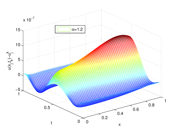
Figure 1: The error surface between the exact solution and numerical solution with $\tau=\frac{1}{50}$ and $h=\frac{1}{200}$.

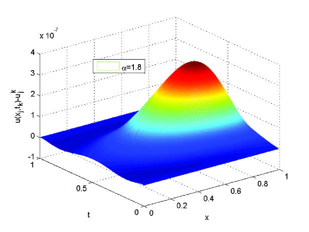
Figure 2: The error surface between the exact solution and numerical solution with $\tau=\frac{1}{100}$ and $h=\frac{1}{1000}$.

5 Conclusion

In this paper, a class of new numerical schemes are proposed for Riemann-Liouville derivatives (and Riesz derivatives). Application of the 2nd-order scheme in spatial direction and the Crank-Nicolson technique in temporal direction, a finite difference scheme is developed to solve the Riesz space fractional advection diffusion equation. We prove that the difference scheme is unconditionally stable and convergent by using the energy method. Finally, two numerical examples have been given to show the effectiveness of the numerical schemes. Following this idea, the method and technique can be extended in a straightforward way to construct much higher-order numerical algorithms for the tempered and substantial fractional derivatives, and the corresponding fractional differential equations.

Appendix A

Now we present cases $p=3$ and $p=4$ in details.

$\mathrm{(i)}$ $p=3$

The generating function with coefficients $\displaystyle\kappa_{3,\ell}^{(\alpha)}\;\left(\ell=0,1,\ldots,\right)$ reads as,

$$\begin{array}[]{lll}\displaystyle\widetilde{W}_{3}(z)=\left(a_{31}+a_{32}z+a_{33}z^{2}+a_{34}z^{3}\right)^{\alpha}=\sum\limits_{\ell=0}^{\infty}\kappa_{3,\ell}^{(\alpha)}z^{\ell},\end{array}$$

where

$$\begin{array}[]{lll}\displaystyle a_{31}=\frac{11\alpha^{2}-12\alpha+3}{6\alpha^{2}},\;\;a_{32}=\frac{-6\alpha^{2}+10\alpha-3}{2\alpha^{2}},\vspace{0.2 cm}\\ \displaystyle a_{33}=\frac{3\alpha^{2}-8\alpha+3}{2\alpha^{2}},\;\;a_{34}=\frac{-2\alpha^{2}+6\alpha-3}{6\alpha^{2}}.\end{array}$$

This generating function can be also rewritten as

$$\begin{array}[]{lll}\displaystyle\widetilde{W}_{3}(z)&=&\displaystyle\left(a_{31}+a_{32}z+a_{33}z^{2}+a_{34}z^{3}\right)^{\alpha}=a_{31}^{\alpha}\left(1-z\right)^{\alpha}\left(1+b_{31}z+b_{32}z^{2}\right)^{\alpha}\vspace{0.4 cm}\\ \displaystyle&=&\displaystyle a_{31}^{\alpha}\left(1-z\right)^{\alpha}\sum\limits_{\ell_{1}=0}^{\infty}\left(\alpha\atop\ell_{1}\right)\left(b_{31}z\right)^{\ell_{1}}\left(1+\frac{b_{32}}{b_{31}}z\right)^{\ell_{1}}\vspace{0.4 cm}\\ \displaystyle&=&\displaystyle a_{31}^{\alpha}\left(1-z\right)^{\alpha}\sum\limits_{\ell_{1}=0}^{\infty}\left(\alpha\atop\ell_{1}\right)\left(b_{31}z\right)^{\ell_{1}}\sum\limits_{\ell_{2}=0}^{\ell_{1}}\left(\ell_{1}\atop\ell_{2}\right)\left(\frac{b_{32}}{b_{31}}z\right)^{\ell_{2}}\vspace{0.4 cm}\\ \displaystyle&=&\displaystyle a_{31}^{\alpha}\sum\limits_{\ell=0}^{\infty}\left[\sum\limits_{\ell_{1}=0}^{\ell}\sum\limits_{\ell_{2}=0}^{\left[\frac{1}{2}\ell_{1}\right]}\frac{\left(-1\right)^{\ell_{1}+\ell_{2}}(\ell_{1}-\ell_{2})!b_{31}^{\ell_{1}-2\ell_{2}}b_{32}^{\ell_{2}}}{\ell_{2}!(\ell_{1}-2\ell_{2})!}{\varpi}_{1,\ell-\ell_{1}}^{(\alpha)}{\varpi}_{1,\ell_{1}-\ell_{2}}^{(\alpha)}\right]z^{\ell},\end{array}$$

in which

$$\begin{array}[]{lll}\displaystyle b_{31}=\frac{-7\alpha^{2}+18\alpha-6}{11\alpha^{2}-12\alpha+3},\;\;b_{32}=\frac{2\alpha^{2}-6\alpha+3}{11\alpha^{2}-12\alpha+3}.\end{array}$$

So,

$$\begin{array}[]{lll}\displaystyle\kappa_{3,\ell}^{(\alpha)}=a_{31}^{\alpha}\sum\limits_{\ell_{1}=0}^{\ell}\sum\limits_{\ell_{2}=0}^{\left[\frac{1}{2}\ell_{1}\right]}P(\alpha,\ell_{1},\ell_{2}){\varpi}_{1,\ell-\ell_{1}}^{(\alpha)}{\varpi}_{1,\ell_{1}-\ell_{2}}^{(\alpha)},\;\ell=0,1,\ldots.\end{array}$$

where

$$\begin{array}[]{lll}\displaystyle P(\alpha,\ell_{1},\ell_{2})=\frac{\left(-1\right)^{\ell_{1}+\ell_{2}}(\ell_{1}-\ell_{2})!}{\ell_{2}!(\ell_{1}-2\ell_{2})!}b_{31}^{\ell_{1}-2\ell_{2}}b_{32}^{\ell_{2}}.\end{array}$$

In addition, we can get the following recursion relation by using the expressions of $\kappa_{3,\ell}^{(\alpha)}$ and automatic differentiation techniques,

$$\left\{\begin{array}[]{lll}\displaystyle\kappa_{3,0}^{(\alpha)}&=&\displaystyle\left(\frac{11\alpha^{2}-12\alpha+3}{6\alpha^{2}}\right)^{\alpha},\vspace{0.2 cm}\\ \displaystyle\kappa_{3,1}^{(\alpha)}&=&\displaystyle-\frac{3\alpha(6\alpha^{2}-10\alpha+3)}{11\alpha^{2}-12\alpha+3}\kappa_{3,0}^{(\alpha)},\vspace{0.2 cm}\\ \displaystyle\kappa_{3,2}^{(\alpha)}&=&\displaystyle\frac{3\alpha(108\alpha^{5}-402\alpha^{4}+520\alpha^{3}-312\alpha^{2}+87\alpha-9)}{2(11\alpha^{2}-12\alpha+3)^{2}}\kappa_{3,0}^{(\alpha)},\vspace{0.2 cm}\\ \displaystyle\kappa_{3,\ell}^{(\alpha)}&=&\displaystyle\frac{1}{a_{31}\ell}\left[a_{32}(\alpha-\ell+1)\kappa_{3,\ell-1}^{(\alpha)}+a_{33}(2\alpha-\ell+2)\kappa_{3,\ell-2}^{(\alpha)}\right.\\ &&\displaystyle\left.+a_{34}(3\alpha-\ell+3)\kappa_{3,\ell-3}^{(\alpha)}\right],\;\ell\geq 3.\end{array}\right.$$

$\mathrm{(ii)}$ $p=4$

The generating function with coefficients $\displaystyle\kappa_{4,\ell}^{(\alpha)}\;\left(\ell=0,1,\ldots,\right)$ reads as follows,

$$\begin{array}[]{lll}\displaystyle\widetilde{W}_{4}(z)=\left(a_{41}+a_{42}z+a_{43}z^{2}+a_{44}z^{3}+a_{45}z^{4}\right)^{\alpha}=\sum\limits_{\ell=0}^{\infty}\kappa_{4,\ell}^{(\alpha)}z^{\ell},\end{array}$$

in which

$$\begin{array}[]{lll}\displaystyle a_{41}=\frac{25\alpha^{3}-35\alpha^{2}+15\alpha-2}{12\alpha^{3}},\;\;a_{42}=\frac{-24\alpha^{3}+52\alpha^{2}-27\alpha+4}{6\alpha^{3}},\vspace{0.2 cm}\\ \displaystyle a_{43}=\frac{6\alpha^{3}-19\alpha^{2}+12\alpha-2}{2\alpha^{3}},\;\;a_{44}=\frac{-8\alpha^{3}+28\alpha^{2}-21\alpha+4}{6\alpha^{3}},\vspace{0.2 cm}\\ \displaystyle a_{45}=\frac{3\alpha^{3}-11\alpha^{2}+9\alpha-2}{12\alpha^{3}}.\end{array}$$

Similarly, one can get

$$\begin{array}[]{lll}\displaystyle\kappa_{4,\ell}^{(\alpha)}=a_{41}^{\alpha}\sum\limits_{\ell_{1}=0}^{\ell}\sum\limits_{\ell_{2}=0}^{\left[\frac{2}{3}\ell_{1}\right]}\sum\limits_{\ell_{3}=\max\{0,2\ell_{2}-\ell_{1}\}}^{\left[\frac{1}{2}\ell_{2}\right]}P(\alpha,\ell_{1},\ell_{2},\ell_{3})\varpi_{1,\ell-\ell_{1}}^{(\alpha)}\varpi_{1,\ell_{1}-\ell_{2}}^{(\alpha)},\end{array}$$

where

$$\begin{array}[]{lll}\displaystyle P(\alpha,\ell_{1},\ell_{2},\ell_{3})=\frac{\left(-1\right)^{\ell_{1}+\ell_{2}}\left(\ell_{1}-\ell_{2}\right)!}{\ell_{3}!\left(\ell_{2}-2\ell_{3}\right)!\left(\ell_{1}+\ell_{3}-2\ell_{2}\right)!}b_{41}^{\ell_{1}+\ell_{3}-2\ell_{2}}b_{42}^{\ell_{2}-2\ell_{3}}b_{43}^{\ell_{3}},\end{array}$$

and

$$\begin{array}[]{lll}\displaystyle b_{41}=\frac{-23\alpha^{3}+69\alpha^{2}-39\alpha+6}{25\alpha^{3}-35\alpha^{2}+15\alpha-2},\;\;b_{42}=\frac{13\alpha^{3}-45\alpha^{2}+33\alpha-6}{25\alpha^{3}-35\alpha^{2}+15\alpha-2},\vspace{0.2 cm}\\ \displaystyle b_{43}=\frac{-3\alpha^{3}+11\alpha^{2}-9\alpha+2}{25\alpha^{3}-35\alpha^{2}+15\alpha-2}.\end{array}$$

The recursion formula is given as,

$$\left\{\begin{array}[]{lll}\displaystyle\kappa_{4,0}^{(\alpha)}=\left(\frac{25\alpha^{3}-35\alpha^{2}+15\alpha-2}{12\alpha^{3}}\right)^{\alpha},\vspace{0.2 cm}\\ \displaystyle\kappa_{4,1}^{(\alpha)}=-\frac{2\alpha(24\alpha^{3}-52\alpha^{2}+27\alpha-4)}{25\alpha^{3}-35\alpha^{2}+15\alpha-2}\kappa_{4,0}^{(\alpha)},\vspace{0.2 cm}\\ \displaystyle\kappa_{4,2}^{(\alpha)}=\frac{2\alpha(576\alpha^{7}-2622\alpha^{6}+4441\alpha^{5}-3835\alpha^{4}+1844\alpha^{3}-497\alpha^{2}+70\alpha-4)}{(25\alpha^{3}-35\alpha^{2}+15\alpha-2)^{2}}\kappa_{4,0}^{(\alpha)},\vspace{0.2 cm}\\ \displaystyle\kappa_{4,3}^{(\alpha)}=-\frac{2\alpha}{3(25\alpha^{3}-35\alpha^{2}+15\alpha-2)^{3}}\left(27648\alpha^{11}-19785\alpha^{10}+591000\alpha^{9}-995240\alpha^{8}\right.\vspace{0.2 cm}\\ \displaystyle\left.\hskip 34.14322pt+1067901\alpha^{7}-775354\alpha^{6}+390051\alpha^{5}-135738\alpha^{4}+31923\alpha^{3}-4820\alpha^{2}\right.\vspace{0.2 cm}\\ \displaystyle\left.\hskip 34.14322pt+420\alpha-16\right)\kappa_{4,0}^{(\alpha)},\vspace{0.2 cm}\\ \displaystyle\kappa_{4,\ell}^{(\alpha)}=\frac{1}{a_{41}\ell}\left[a_{42}(\alpha-\ell+1)\kappa_{4,\ell-1}^{(\alpha)}+a_{43}(2\alpha-\ell+2)\kappa_{4,\ell-2}^{(\alpha)}+a_{44}(3\alpha-\ell+3)\kappa_{4,\ell-3}^{(\alpha)}\right.\vspace{0.2 cm}\\ \left.\hskip 34.14322pt+a_{45}(4\alpha-\ell+4)\kappa_{4,\ell-4}^{(\alpha)}\right],\;\ell\geq 4.\end{array}\right.$$

The cases for $p\geq 5$ can be similarly derived howbeit very complicated. We omit them here.

References

• (1) A. A. Alikhanov, A new difference scheme for the time fractional diffusion equation. J. Comput. Phys. 280 (2015), 424–438.
• (2) W. N. Bailey, Generalized Hypergeometric Series. Stechert-Hafner, Inc., New York, 1964.
• (3) R. H. Chan, Toeplitz Preconditioners for Toeplitz Systems with Nonnegative Generating Functions. IMA J. Numer. Anal. 11 (1991), 333–345.
• (4) R. H. Chan, X. Q. Jin, An Introduction to Iterative Toeplitz Solvers, SIAM, Philadelphia, 2007.
• (5) M. H. Chen, W. H. Deng, WSLD operators: A class of fourth order difference approximations for space Riemann-Liouville derivative, SIAM J. Numer. Anal. 52(2014), 1418–1438.
• (6) S. Chen, J. Shen, L. L. Wang,Generalized Jacobi functions and their applications to fractional differential equations. Math. Comput. in press.
• (7) S. Chen, X. Jiang, F. Liu, I. Turner, High order unconditionally stable difference schemes for the Riesz space-fractional telegraph equation. J. Comput. Appl. Math. 278 (2015), 119–129.
• (8) V. J. Ervin, J. P. Roop, Variational formulation for the stationary fractional advection dispersion equation. Numer. Meth. P. D. E. 22 (2006), 558–576.
• (9) W. Feller, On a generalization of Marcel Riesz’ potentials and the semi-groups generated by them. Comm. Sém. Mathém. Université de Lund. (1952), 73–81.
• (10) R. Garrappaa, I. Moretb, M. Popolizioc, Solving the time-fractional Schrödinger equation by Krylov projection methods. J. Comput. Phys. 293 (2015), 115–134.
• (11) J. Huang, Y. Tang, L. Vázquez, J. Yang, Two finite difference schemes for time fractional diffusion-wave equation. Numer. Algorithms. 64 (2013), 707–720.
• (12) A. A. Kilbas, H. M. Srivastava, J. J.Trujillo, Theory and Applications of Fractional Differential Equations, Elsevier: Amsterdam, the Netherlands, 2006.
• (13) C. Lubich. Discretized fractional calculus. SIAM J. Math. Anal. 17 (1986), 704–719.
• (14) C. P. Li, H. F. Ding, Higher order finite difference method for the reaction and anomalous-diffusion equation. Appl. Math. Model. 38 (2014), 3802–3821.
• (15) K. S. Miller, B. Ross, An Introduction to the Fractional Calculus and Fractional Differential Equations, John Wily and Sons Inc., New York, 1993.
• (16) M. M. Meerschaert, C. Tadjeran, Finite difference approximations for fractional advection-dispersion flow equations. J. Comput. Appl. Math. 172 (2004), 65–77.
• (17) R. Metzler, J. Klafter, The random walk s guide to anomalous diffusion: A fractional dynamics approach. Phys. Rep. 339 (2000), 1–77.
• (18) N. E. Nörlund, Vorlesungen über Differenzenrechnung, Springer, Berlin, 1924.
• (19) K. B. Oldham, J. Spanier, The Fractional Calculus, Academic Press, New York, 1974.
• (20) I. Podlubny, Fractional Differential Equations, Academin Press, San Diego, CA, USA, 1999.
• (21) A. Quarteroni, R. Sacco, F. Saleri, Numerical Mathematics, 2nd edition, Springer, New York, 2007.
• (22) L. B. Rall, Perspectives on automatic differentiation: past, present, and future? Automatic differentiation: applications, theory, and implementations, Springer, Berlin, 2006.
• (23) H. M. Srivastava, An explicit formula for the generalized Bernoulli polynomials. J. Math. Anal. Appl. 130 (1988), 509–513.
• (24) S. G. Samko, A. A. Kilbas, O. I. Marichev, Fractional Integrals and Derivatives, Theory and Applications, Gordon and Breach: London, UK, 1993.
• (25) A. I. Saichev, G. M. Zaslavsky, Fractional kinetic equations: solutions and applications. Chaos. 7 (1997), 753–764.
• (26) F. G. Tricomi, A. Erdélyi, The asymptotic expansion of a ratio of Gamma functions, Pacific J. Math. (1951) 133–142.
• (27) W. Y. Tian, H. Zhou, W. H. Deng, A class of second order difference approximations for solving space fractional diffusion equations. Math. Comput. 84 (2015), 1703–1727.
• (28) H. Wang, N. Du, Fast alternating-direction finite difference methods for three-dimensional space-fractional diffusion equations. J. Comput. Phys. 258 (2014), 305–318.
• (29) Z. Wang, S. Vong, Compact difference schemes for the modified anomalous fractional sub-diffusion equation and the fractional diffusion-wave equation. J. Comput. Phys. 277 (2014), 1–15.
• (30) Q. Xu, J. S. Hesthavenc, F. Chen, A parareal method for time-fractional differential equations. J. Comput. Phys. 293 (2015), 173–183.
• (31) S. B. Yuste, L. Acedo, An explicit finite difference method and a new von Neumann-type stability analysis for fractional diffusion equations. SIAM J. Numer. Anal. 42 (2005), 1862–1874.
• (32) M. Zayernouri, G. Em Karniadakis, Fractional spectral collocation method. SIAM J. Sci. Comput. 36 (2014), A40–A62.
• (33) F. H. Zeng, C. P. Li, F. W. Liu, I. Turner, The use of finite difference/element approaches for solving the time-fractional subdiffusion equation. SIAM J. Sci. Comput. 35 (2013), A2976–A3000.
• (34) X. Zhao, Z. Z. Sun, Compact Crank-Nicolson schemes for a class of fractional Cattaneo equation in inhomogeneous medium. J. Sci. Comput. 62 (2015), 747–771.