Leading hadronic contributions to the running of the electroweak coupling constants from lattice QCD

Abstract

The quark-connected leading-order hadronic contributions to the running of the electromagnetic fine structure constant, $\alpha_{\rm QED}$, and the weak mixing angle, $\theta_{W}$, are determined by a four-flavour lattice QCD computation with twisted mass fermions. Full agreement of the results with a phenomenological analysis is observed with an even comparable statistical uncertainty. We show that the uncertainty of the lattice calculation is dominated by systematic effects which then leads to significantly larger errors than obtained by the phenomenological analysis.

1 Introduction

Finding hints for new physics beyond the standard model (SM) has been a major objective of particle physics over the past decades. A very promising strategy to detect such effects are high precision experimental measurements which are matched by equally precise theoretical predictions. An important ingredient for the precision attainable in a theoretical calculation is the knowledge of the coupling constants since they enter the quantum loop corrections.

In this article, we investigate the leading-order hadronic contributions for two of these couplings, the electromagnetic fine structure constant, $\alpha_{\rm QED}$, and the $SU(2)_{L}$ coupling constant, $\alpha_{2}$, both related by the weak mixing angle, $\theta_{W}$. An accurate knowledge of these hadronic contributions is mandatory to accomplish sufficiently precise predictions for future high-energy colliders Jegerlehner:2011mw or low energy experiments Hewett:2012ns .

However, the hadronic contributions to the running of $\alpha_{\rm QED}$ turn out to be only poorly known at the scale of the Z-boson mass. Compared to $\alpha_{\rm QED}$ at zero momentum transfer, there is a five orders of magnitude loss of precision when $\alpha_{\rm QED}$ is taken at the Z-scale turning $\alpha_{\rm QED}(M_{Z}^{2})$ into one of the least determined input parameters of the standard model Hagiwara:2011af .

Phenomenologically, the leading hadronic contribution to the running of $\alpha_{\rm QED}$ originating from hadronic vacuum polarisation effects, $\Delta\alpha_{\rm QED}^{\rm hvp}$, is determined from a dispersion relation and experimental $e^{+}e^{-}$ scattering data for the hadronic cross-sections Jegerlehner:2008rs ; Jegerlehner:2011mw ; Hagiwara:2011af . Although new data has recently become available, the present analysis does not lead to a sufficient improvement of the error which would be needed for the requirements of future collider experiments Hagiwara:2011af .

In principle, lattice QCD calculations would be an ideal tool to determine the hadronic contributions to electroweak observables such as $\alpha_{\rm QED}$ or $\alpha_{2}$ considered here. However, presently the precision that can be obtained from such lattice QCD computations is usually still lower than from the phenomenological analyses. Nevertheless, the steady progress which is taking place in lattice QCD calculations promises to make it an expedient alternative to the phenomenological results in the future. In fact, as we will demonstrate here, even with our present simulations the statistical uncertainty already matches the phenomenological error of $\Delta\alpha_{\rm QED}^{\rm hvp}$ and $\Delta^{\rm hvp}\sin^{2}\theta_{W}$.

$\Delta\alpha_{\rm QED}^{\rm hvp}$ has first been investigated on the lattice for two dynamical twisted mass fermions Renner:2012fa . Preliminary results incorporating also dynamical strange and charm quarks for one selected momentum value have been reported in Feng:2012gh . Another determination of $\Delta\alpha_{\rm QED}^{\rm hvp}$, following the approach suggested in Jegerlehner:2008rs has been performed in Francis:2014yga .

Here, we present our results obtained on the $N_{f}=2+1+1$ ensembles of the European twisted mass collaboration Baron:2010bv ; Baron:2010th . We will include an estimate of the systematic uncertainties originating from the continuum limit and from the extrapolation to the physical point for energies ranging from $0$ to $10\,{\rm GeV}^{2}$.

In contrast to $\Delta\alpha_{\rm QED}^{\rm hvp}$, the hadronic contributions to the running of the weak mixing angle, $\theta_{W}$, have not been studied on the lattice so far. Such a calculation is important since the phenomenological determination at low energies cannot only be based on data but also needs some assumptions such as a partial flavour separation of the cross-section data Jegerlehner:1985gq .

Lattice calculations can, in contrast, provide a first-principle evaluation of the weak mixing angle in the low-momentum region, where several measurements exist Wood:1997zq ; Anthony:2005pm ; Wang:2014bba ; Armstrong:2014tna . In addition, due to the great potential of such low energy experiments for unveiling the nature of physics beyond the SM, there are also newly planned experimental facilities Benesch:2014bas ; Chen:2014psa ; Becker:2013fya , see also Kumar:2013yoa for a discussion on such experiments. Here, we present the first lattice QCD calculation of the leading hadronic contribution to the weak mixing angle, $\Delta^{\rm hvp}\sin^{2}\theta_{W}$.

2 The fine structure constant $\alpha_{\rm QED}$

Radiative corrections lead to charge renormalisation and thus to the running of the fine structure constant obtained by summing the one-particle irreducible bubble insertions in the photon propagator Jegerlehner:1985gq

$$\alpha_{\mathrm{QED}}(Q^{2})=\frac{\alpha_{0}}{1-\Delta\alpha_{\mathrm{QED}}(Q^{2})}\;\mathrm{.}$$ (1)

Here, $\alpha_{0}$ is the value at vanishing momentum transfer $Q^{2}=0$, $\alpha_{0}^{-1}=137.035999173(35)$ Aoyama:2012wj . The leading-order hadronic contribution is given by Jegerlehner:2011mw

$$\Delta\alpha_{\mathrm{QED}}^{\mathrm{hvp}}(Q^{2})=-4\pi\alpha_{0}\Pi_{\mathrm{R}}\left(Q^{2}\right)$$ (2)

and is thus proportional to the subtracted vacuum polarisation function

$$\Pi_{\mathrm{R}}(Q^{2})=\Pi(Q^{2})-\Pi(0)\;.$$ (3)

As mentioned in the introduction, this is usually Jegerlehner:1985gq ; Aoyama:2012wj ; Jegerlehner:2011mw determined by a phenomenological approach relying on the once-subtracted dispersion relation Jegerlehner:2009ry which for Euclidean momenta $Q^{2}$ reads

$$\Pi_{\mathrm{R}}(Q^{2})=\frac{\alpha_{0}}{3\pi}\,Q^{2}\,\int_{0}^{\infty}ds\frac{R_{\rm had}(s)}{s(s+Q^{2})}$$ (4)

and experimental cross-section data for

$$R_{\rm had}(s)=\frac{\sigma(e^{+}e⁻\rightarrow{\rm hadrons})}{\frac{4\pi\alpha_{\rm QED}^{2}(s)}{3s}}\,.$$ (5)

Lattice QCD represents an ab-initio alternative for the calculation of $\Pi_{\mathrm{R}}(Q^{2})$, since the hadronic vacuum polarisation tensor can be obtained directly in Euclidean space-time from the correlator of two electromagnetic vector currents.

2.1 Lattice calculation

Ensemble	$\beta$	$a[{\rm fm}]$	$\left(\frac{L}{a}\right)^{3}\times\frac{T}{a}$	$m_{PS}$[MeV]	$L$[fm]	$N_{\mathrm{conf}}$
D15.48	$2.10$	$0.061$	$48^{3}\times 96$	227	2.9	$265/155/156$
D30.48	$2.10$	$0.061$	$48^{3}\times 96$	318	2.9	$203/148/148$
D45.32sc	$2.10$	$0.061$	$32^{3}\times 64$	387	1.9	$397/346/346$
B25.32t	$1.95$	$0.078$	$32^{3}\times 64$	274	2.5	$273/179/180$
B35.32	$1.95$	$0.078$	$32^{3}\times 64$	319	2.5	$201/194/194$
B35.48	$1.95$	$0.078$	$48^{3}\times 96$	314	3.7	$235/103/104$
B55.32	$1.95$	$0.078$	$32^{3}\times 64$	393	2.5	$225/125/125$
B75.32	$1.95$	$0.078$	$32^{3}\times 64$	456	2.5	$158/100/100$
B85.24	$1.95$	$0.078$	$24^{3}\times 48$	491	1.9	$192/142/136$
A30.32	$1.90$	$0.086$	$32^{3}\times 64$	283	2.8	$267/158/158$
A40.32	$1.90$	$0.086$	$32^{3}\times 64$	323	2.8	$248/174/174$
A50.32	$1.90$	$0.086$	$32^{3}\times 64$	361	2.8	$216/147/157$

Table 1: Parameters of the $N_{f}=2+1+1$ flavour gauge field configurations that have been analysed in this work. $\beta$ denotes the gauge coupling, $a$ the lattice spacing, $\left(\frac{L}{a}\right)^{3}\times\frac{T}{a}$ the space-time volume and $m_{PS}$ is the value of the light pseudoscalar meson mass. The values for $m_{PS}$ have been determined in Baron:2010bv . $L$ is the spatial extent of the lattices. The lattice spacings are taken from Baron:2011sf . The last column gives the number of statistically independent gauge configurations used to estimate the light/strange/charm contribution to the polarisation function.

The strategy for computing and analysing the hadronic vacuum polarisation function is the same as in Burger:2013jya ; Burger:2015oya . In particular, we employ the same set of ensembles Baron:2010bv ; Baron:2010th , which is presented in table 1. Additionally, we have checked our chiral extrapolations of the light quark contribution by comparing the results with those obtained on a $N_{f}=2$ ensemble featuring the physical pion mass Abdel-Rehim:2013yaa ; Abdel-Rehim:2014nka ; Abdel-Rehim:2015pwa . The parameters of this ensemble are given in table 2.

$\beta$	$c_{\rm SW}$	$a[{\rm fm}]$	$\left(\frac{L}{a}\right)^{3}\times\frac{T}{a}$	$m_{PS}$[MeV]	$L$[fm]	$N_{\rm conf}$
$2.10$	$1.57551$	$0.094$	$48^{3}\times 96$	128	4.6	804

Table 2: Parameters of ensemble featuring $N_{f}=2$ twisted mass fermions at the physical point.

As in Burger:2013jya ; Burger:2015oya , we use the conserved point-split vector current at source and sink and we restrict our considerations to the quark-connected contributions. In this case, the total vacuum polarisation function

$$\Pi^{\rm tot}(Q^{2})=\frac{5}{9}\Pi^{\rm ud}(Q^{2})+\frac{1}{9}\Pi^{\rm s}(Q^{2})+\frac{4}{9}\Pi^{\rm c}(Q^{2})$$ (6)

is obtained by summing the single-flavour contributions which we define without the charge factors.

For each ensemble and each flavour $\rm f$, we first fit the temporal vector current correlator to determine the vector meson masses, $m_{i}$, and their couplings, $g_{i}$. Then we fit the hadronic vacuum polarisation function obtained from the current correlator as detailed in Burger:2013jya to the following functional form

$$\Pi^{\rm f}(Q^{2})=(1-\Theta(Q^{2}-Q^{2}_{\rm match}))\Pi^{\rm f}_{\mathrm{low}}(Q^{2})+\Theta(Q^{2}-Q^{2}_{\rm match})\Pi^{\rm f}_{\mathrm{high}}(Q^{2})\;,$$ (7)

where $\Theta(x)$ is the Heaviside step function. The low-momentum fit function for $0\leq Q^{2}\leq Q^{2}_{\rm match}$ is given by

$$\Pi^{\rm f}_{\mathrm{low}}(Q^{2})=\sum_{i=1}^{M}\frac{g^{2}_{i}m^{2}_{i}}{m^{2}_{i}+Q^{2}}+\sum_{j=0}^{N-1}a_{j}(Q^{2})^{j}\;,$$ (8)

and the high-momentum piece for $Q^{2}_{\rm match}\leq Q^{2}\leq Q_{\rm max}^{2}$ reads

$$\Pi^{\rm f}_{\mathrm{high}}(Q^{2})=\log(Q^{2})\sum_{k=0}^{B-1}b_{k}(Q^{2})^{k}+\sum_{l=0}^{C-1}c_{l}(Q^{2})^{l}\;.$$ (9)

The number of terms and thus the fit function is characterised by M, N, B, and C. The ansatz in Eq. (8) consists of three parts: a series of poles at energies $m_{i}$ and with residual $g_{i}^{2}m_{i}^{2}$, $i=1,\ldots,M$, an additive constant $a_{0}$ and further polynomial terms $a_{i}\,(Q^{2})^{i}$ for $i\geq 1$. The poles characterised by $(m_{i},g_{i})$ are identified with the exponential contributions to the time-dependent vector-current 2-point correlation function at zero spatial momentum. This is the reason why the parameters $(m_{i},g_{i})$ are obtained from a fit of the latter and inserted into the fit of the vacuum polarisation function under preservation of all error correlations. The ansatz in Eq. (8) is valid for any four-momentum $Q^{2}$, in particular for $Q=\left(Q_{0},\vec{Q}=0\right)$ with $Q^{2}=Q^{2}_{0}$. Given such a momentum configuration, the above identification follows from the Fourier transform of the polarisation tensor. With the limited statistical precision of the 2-point vector correlator, the number of exponentials we can resolve in practice is limited to 2. Contributions from states with even larger energies are effectively accounted for by the polynomial terms.

The ansatz in Eq. (9) is chosen to provide an adequate parametrisation of the polarisation function. This is the only requirement in the high-momentum region $Q^{2}_{\mathrm{match}}<Q^{2}\leq Q^{2}_{\mathrm{max}}$. While in the low-momentum region the extrapolation beyond the lowest non-zero lattice momentum to zero momentum is of physical significance as it predicts the curvature of the polarisation function in this interval, in the high-momentum region we only need the ansatz in Eq. (9) to interpolate the available lattice data.

In the following, we use $Q^{2}_{\rm max}=100\,{\rm GeV}^{2}$ and choose $Q^{2}_{\rm match}=2\,{\rm GeV}^{2}$. Varying $Q^{2}_{\rm match}$ by $1\,{\rm GeV}^{2}$ to the left and to the right gives compatible results. We perform extrapolations of the subtracted polarisation function in the light quark mass and the lattice spacing only for momenta in the interval $0<Q^{2}\leq 10\,{\rm GeV}^{2}$ since for larger $Q^{2}$ perturbative calculations are expected to yield more precise determinations.

Since our four-flavour ensembles feature unphysically large pion masses, an extrapolation to the physical point has to be performed. The pion mass dependence of the single-flavour contributions can be assessed by looking at the leading vector meson contribution obtained in chiral perturbation theory Ecker:1988te ; Aubin:2006xv

$$\Pi^{\rm f}(Q^{2})=g_{V}^{2}\frac{m_{V}^{2}}{Q^{2}+m_{V}^{2}}\;.$$ (10)

The spectral properties of the heavy vector mesons hardly depend on the pion mass and also the coupling constant $g_{V}$ of the $\rho$-meson has been found to be well-described by a linear fit in the squared pion mass, $m_{\rm PS}^{2}$, cf. Renner:2012fa . However, the $\rho$-meson mass, $m_{V}$, strongly depends on the value of the light quark masses, taken to be degenerate in our calculation, and thus the squared pion mass Burger:2013jya . This is illustrated in Fig. 1 left by a model extrapolation which is constrained by requiring the $\rho$-meson mass to attain its experimental value Agashe:2014kda at the physical point, similarly to the one used in the two-flavour case in Ref. Feng:2011zk .

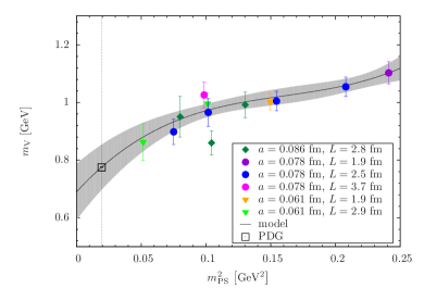
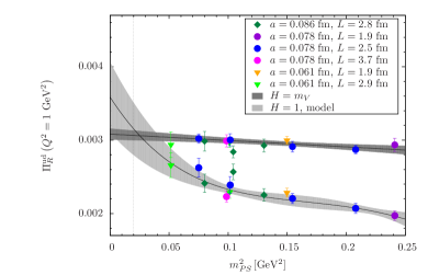
Figure 1: Left: Dependence of $\rho$-meson mass, $m_{V}$, on the squared pion mass, $m_{\rm PS}^{2}$, determined on the $N_{f}=2+1+1$ twisted mass ensembles shown in table 1. Right: Chiral extrapolation of the renormalised light-quark vacuum polarisation function at a generic value of $Q^{2}=1\,{\rm GeV}^{2}$ obtained with the redefinition given in Eq. (11) (upper set of data points) and with the standard definition Eq. (3) (lower set of data points). For the latter the same model extrapolation as for the $\rho$-meson mass has been used.

Eq. (LABEL:.) (10) implies that a similar non-linear behaviour can be expected for the light-quark hadronic vacuum polarisation function as we indeed observe for the lower set of data points in Fig. 1 right. From Eq. (10) we also see that we can eliminate this non-linear dependence on the squared pion mass to a large extent by employing the lattice redefinition presented in Ref. Renner:2012fa for the light-quark contribution to the vacuum polarisation function,

$$\bar{\Pi}_{R}^{\rm ud}\left(Q^{2}\right)=\Pi^{\rm ud}_{R}\left(Q^{2}\cdot\frac{H^{2}}{H_{\mathrm{phys}}^{2}}\right)\,,$$ (11)

if we use $H=m_{V}$, i.e. the $\rho$-meson mass at unphysically large up and down quark masses. The beneficial effect this has on the data points is depicted as the upper set of data points in Fig. 1 right. Hence, in the following we use the above redefinition in the light-quark sector. For the contributions of the heavy quark flavours, we use the standard definition of the vacuum polarisation function $\Pi^{\rm f}_{R}(Q^{2})$, ${\rm f}={\rm s,c}$. Our redefinition of the total $\Delta\alpha_{\mathrm{QED}}^{\mathrm{hvp}}$ then follows from the sum over all quark flavours as in Eq. (6)

$$\Delta\overline{\alpha}_{\mathrm{QED}}^{\mathrm{hvp}}(Q^{2})=-4\pi\alpha_{0}\,\left(\frac{5}{9}\,\Pi^{\rm ud}_{\mathrm{R}}\left(Q^{2}\cdot\frac{H^{2}}{H_{\mathrm{phys}}^{2}}\right)+\frac{1}{9}\,\Pi^{\rm s}_{\mathrm{R}}\left(Q^{2}\right)+\frac{4}{9}\,\Pi^{\rm c}_{\mathrm{R}}\left(Q^{2}\right)\right)\,.$$ (12)

The lattice data obtained with the definition $\Delta\overline{\alpha}_{\mathrm{QED}}^{\mathrm{hvp}}$ in Eq. (12) can be sufficiently well described already by a linear dependence on the squared pion mass. Since we use only this definition throughout this work and no confusion is possible, we henceforth omit the bar in $\Delta\overline{\alpha}_{\mathrm{QED}}^{\mathrm{hvp}}$.

2.2 Results

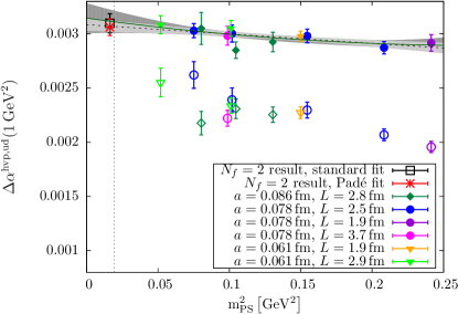
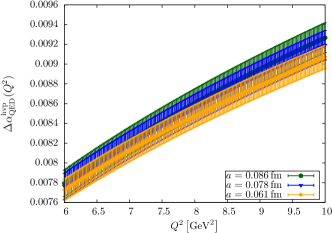
Figure 2: Left: Light-quark contribution to $\Delta\alpha_{\rm QED}^{\rm hvp}$ with filled symbols representing points obtained with Eq. (11) using $H=m_{V}$, open symbols refer to those obtained with Eq. (2), i. e. $H=1$ in Eq. (11). In particular, the two-flavour results at the physical point have been computed with the standard definition. The light grey errorband displays the uncertainty of the linear fit represented by the black dotted line, wheras the dark grey errorband belongs to a quadratic fit represented by the green solid line. Right: $N_{f}=2+1+1$ contribution to $\Delta\alpha_{\rm QED}^{\rm hvp}$ for the three lattice spacings at a fixed pion mass of $m_{\rm PS}\approx 320\,{\rm MeV}$.

In order to show that the above redefinition in Eq. (11) indeed provides the expected benefit for the chiral extrapolation of the light quark contribution to the running of the fine structure constant, we show the data for both Eqs. (2) and (11) with $H=m_{V}$ in Fig. 2 left for a single momentum value $Q^{2}=1\,{\rm GeV}^{2}$. The upper set of data points obtained with the redefinition Eq. (11) evidently is much easier to extrapolate to the physical value of the pion mass than the lower points procured from the standard definition Eq. (2).

Since we do neither observe lattice spacing artefacts nor finite size effects in these data at $Q^{2}=1\,{\rm GeV}^{2}$, we can actually compare our results computed on the four-flavour ensembles linearly extrapolated in the squared pion mass, $m_{\rm PS}^{2}$, with those obtained from the $N_{f}=2$ ensemble featuring the physical pion mass. Additionally to the standard analysis, we have performed a correlated $[1,1]$ Padé fit Aubin:2012me , possessing the same number of parameters, up to $Q^{2}_{\rm max}=1.5\,{\rm GeV}^{2}$ such that $Q^{2}=1\,{\rm GeV}^{2}$ is safely covered. As expected, the values for the pole parameters determined from the temporal correlator in our standard approach and from the Padé fit are compatible

$$a^{2}\,m_{V}^{2}=0.153(35)\qquad b_{n}=0.1575(81)$$ (13)

and also the results of both analyses of the leading hadronic contribution to the running of the fine structure constant at the physical point completely agree with each other and with the extrapolated result obtained on the four-flavour ensembles indicating that the systematic uncertainty caused by the chiral extrapolation is small. The results at the physical value of the pion mass, which are depicted in the left panel of Fig. 2, are summarised in table 3.

$N_{f}=2+1+1$ extrapolated	$N_{f}=2$ standard	$N_{f}=2$ $[1,1]$ Padé
0.003068(50)	0.003097(88)	0.003062(77)

Table 3: Comparison of the chirally extrapolated result for $\Delta\alpha_{\rm QED}^{\rm hvp,ud}(1\,{\rm GeV}^{2})$ obtained on the $N_{f}=2+1+1$ ensembles with those obtained on the $N_{f}=2$ ensemble at the physical point. For the latter, we have performed our standard analysis but without the redefinition and also tested a [1,1] Padé fit.

Including also the heavy quark contributions by using Eq. (12), a dependence on the lattice spacing is clearly visible, especially in the high-$Q^{2}$ region shown in the right panel of Fig. 2. This is accounted for by combining the chiral extrapolation with taking the continuum limit and employing the following fit function to the four-flavour results obtained on individual ensembles

$$\Delta\alpha_{\mathrm{QED}}^{\mathrm{hvp}}(Q^{2})(m_{\rm PS},a)=A+B~{}m_{\rm PS}^{2}+C~{}a^{2}$$ (14)

with fit parameters $A$, $B$, $C$ for each momentum value $Q^{2}\in\{0,0.02,0.04,\ldots,10\}\,{\rm GeV}^{2}$. In Burger:2014ada we have shown that automatic $\mathcal{O}(a)$ improvement is at work for our definition of the hadronic vacuum polarisation function. Thus, performing the continuum extrapolation without a term linear in the lattice spacing $a$ in Eq. (14) is justified. The ansatz in Eq. (14) neglects any dependence on the finite lattice extent which has been found to be smaller than our current statistical uncertainties and will be discussed when assessing the systematic effects of our calculations.

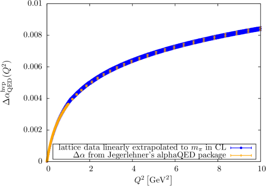
Figure 3: $N_{f}=2+1+1$ contribution to $\Delta\alpha_{\rm QED}^{\rm hvp}$ compared to the data collected in Jegerlehner:2012:Online employing the dispersion relation in Eq. (4). The lattice data are taken at the physical point and in the continuum limit (CL).

The results are depicted in Fig. 3 together with the results obtained by a phenomenological analysis Jegerlehner:2011mw . Here, for both the lattice calculation and the phenomenological analysis only the statistical errors are shown. Over the whole momentum range, perfect agreement with comparable statistical uncertainties is found. We will discuss the systematic uncertainties of our lattice QCD determination below. An updated phenomenological analysis including all data published till the end of 2014 will soon be available Jegerlehner:2015 . The lattice data also agree with those results featuring even smaller uncertainties.

2.2.1 Systematic uncertainty from the choice of vector meson fit ranges

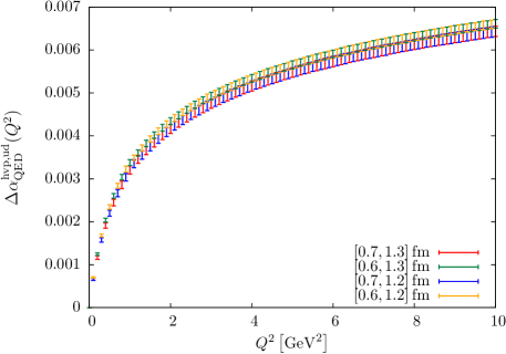
Figure 4: Light quark contribution to $\Delta\alpha_{\rm QED}^{\rm hvp}$ obtained with different fit ranges for the $\rho$-meson mass, $m_{V}$ and coupling, $g_{V}$. The standard fit range is $[0.7\,{\rm fm},1.2\,{\rm fm}]$.

As mentioned before, the first step in our analysis is the determination of the masses and the coupling constants of the vector mesons from the vector two-point functions at zero momentum. The values of the spectral parameters differ when varying the fit range. We have repeated the complete analysis for various vector meson fit ranges for the light, strange and charm quark currents propagating the uncertainty to the final results.

In the light quark sector depicted in Fig. 4, we observe systematic uncertainties depending on whether we start fitting the vector meson correlator at $0.6\,{\rm fm}$ or at $0.7\,{\rm fm}$ whereas changing the upper border of the fit interval by $0.1\,{\rm fm}$ does not lead to observable effects. The dependence on the lower starting point of the fit can be attributed to excited state contamination of the $\rho$-meson correlator. When stating the final results for selected momentum values below, we take for these systematic uncertainties half the difference between the central values that are furthest apart from each other.

For the heavy flavours changing the fit interval by $0.1\,{\rm fm}$ to the left and to the right of both the lower and the upper time slice of the fit ranges does not lead to observable differences. This is shown in Fig. 5.

Figure 5: Dependence of the single-flavour contributions to $\Delta\alpha_{\rm QED}$ on the fit range of the $\overline{s}s$-correlator (left panel) and of the $J/\Psi$-correlator (right panel). The standard $\overline{s}s$-correlator fit range is $[0.9\,{\rm fm},1.4\,{\rm fm}]$, whereas the one for the charm quark correlator is $[1.2\,{\rm fm},1.7\,{\rm fm}]$. The minor discontinuities at $Q^{2}=2\,{\rm GeV}^{2}$ arise from connecting the low-momentum Eq. (8) and high-momentum Eq. (9) fit functions at this point by a simple step function as shown in Eq. (7). Due to the subdominance of the heavy flavour contributions, those discontinuities do not influence the final result.

2.2.2 Systematic uncertainty from the choice of vacuum polarisation fit function

Performing the whole analysis with different numbers of terms in our vacuum polarisation fit functions also leads to observable differences in the light quark contribution as shown in Fig. 6. These are larger than the effects from the fit ranges of the vector meson fits discussed in the preceding subsection and thus present the dominant systematic uncertainty in our calculation. It might be possible to improve the situation by e.g. the method of analytic continuation Feng:2013xsa ; Francis:2013fzp or by taking momentum derivatives of the vacuum polarisation function deDivitiis:2012vs .

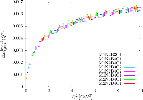
Figure 6: Light quark contribution to $\Delta\alpha_{\rm QED}^{\rm hvp}$ obtained from different fit functions. The standard fit is M1N2B4C1.

The situation for the heavy quarks is shown in Fig. 7. Here, almost no systematic deviations are visible. Furthermore the contributions from the heavy quarks are about an order of magnitude smaller than the light-quark one. Hence, we do not take systematic effects from the variation of the second-generation quark fit functions into account in our final error estimate.

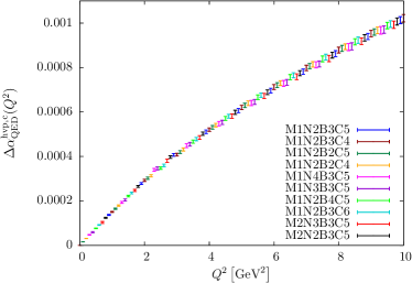
Figure 7: Dependence of the single-flavour contributions to $\Delta\alpha_{\rm QED}$ on the choice of fit function for the strange (left panel) and for the charm (right panel) quark pieces. For the strange quark the standard fit is M1N2B4C1, whereas the one for the charm quark correlator is M1N2B3C5.

2.2.3 Finite size effects

In lattice QCD, typically $m_{\mathrm{PS}}~{}L\gtrsim 4$ is required to minimise systematic effects due to the finite lattice volumes, where $L$ denotes the spatial extent of the lattice. The $N_{f}=2+1+1$ ensembles analysed in this work feature $3.35<m_{\mathrm{PS}}~{}L<5.93$. Restricting our data to the condition $m_{\rm PS}L>3.8$ yields the picture shown in the left panel of Fig. 8. Hence, we do not associate a systematic uncertainty to the usage of ensembles possessing smaller $m_{\rm PS}L$ values.

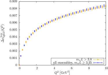
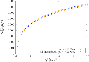
Figure 8: Four-flavour contribution to $\Delta\alpha_{\rm QED}^{\rm hvp}$ obtained with (left panel) $m_{\rm PS}L\geq 3.35$ [standard] and $m_{\rm PS}L>3.8$ and (right panel) $m_{\rm PS}\leq 491\,{\rm MeV}$ [standard] and $m_{\rm PS}L<400\,{\rm MeV}$.

2.2.4 Systematic uncertainty from including heavy pion masses

In order to extrapolate to the physical point, $m_{\pi}\approx 140\,{\rm MeV}$, often not too high pion masses should be included in the fit. The ensembles entering the standard analysis comprise pion masses up to $m_{\rm PS}\approx 491\,{\rm MeV}$. Using only the ensembles with $m_{\rm PS}<400\,{\rm MeV}$ yields fully compatible results for $\Delta\alpha_{\rm QED}^{\rm hvp}$ as can be seen in the right panel of Fig. 8. Therefore, we do not account for a systematic uncertainty related to the usage of pion masses above $400\,{\rm MeV}$.

2.2.5 Final results for selected momentum values

Table 4 contains our final results compared to those of a phenomenological analysis Jegerlehner:2011mw utilising the once-subtracted dispersion relation Eq. (4). The first error denotes the statistical and the second error the systematic uncertainty of our results. The latter constitutes the dominant source of uncertainty of which the biggest part originates from the choice of the vacuum polarisation fit function. This might change when lowering the statistical uncertainty, because then the vacuum polarisation fit gets more constrained. Alternatively, avoiding to fit the vacuum polarisation might be considered.

$Q^{2}$ [$\rm GeV^{2}$]	this work	dispersive analysis Jegerlehner:2011mw
0.02	$0.163\,(05)\,(09)\cdot 10^{-3}$	$0.174\,(02)\cdot 10^{-3}$
1.00	$3.721\,(96)\,(145)\cdot 10^{-3}$	$3.651\,(40)\cdot 10^{-3}$
2.00	$4.993\,(102)\,(144)\cdot 10^{-3}$	$4.916\,(61)\cdot 10^{-3}$
3.00	$5.800\,(111)\,(151)\cdot 10^{-3}$	$5.725\,(74)\cdot 10^{-3}$
4.00	$6.396\,(108)\,(156)\cdot 10^{-3}$	$6.333\,(84)\cdot 10^{-3}$
6.00	$7.264\,(114)\,(159)\cdot 10^{-3}$	$7.223\,(98)\cdot 10^{-3}$
8.00	$7.906\,(124)\,(151)\cdot 10^{-3}$	$7.850\,(107)\cdot 10^{-3}$
10.0	$8.419\,(130)\,(159)\cdot 10^{-3}$	$8.420\,(114)\cdot 10^{-3}$

Table 4: We tabulate $\Delta\alpha_{\rm QED}^{\rm hvp}(Q^{2})$ for selected values of $Q^{2}$. The first error of the lattice results is statistical, the second systematic. The phenomenological values of $\Delta\alpha_{\rm QED}^{\rm hvp}(Q^{2})$ have been obtained from the dispersive analysis of Ref. Jegerlehner:2011mw .

3 The weak mixing angle $\sin^{2}\theta_{W}$

The weak mixing or Weinberg angle, $\theta_{W}$, is one of the fundamental parameters of the electroweak standard model defined by

$$\sin^{2}\theta_{W}=\frac{g^{\prime 2}}{g^{\prime 2}+g^{2}}=\frac{e^{2}}{g^{2}}=\frac{\alpha_{\rm QED}}{\alpha_{2}}$$ (15)

where $g$ is the $SU(2)_{L}$ coupling constant and $g^{\prime}$ the $U(1)_{Y}$ coupling constant. The second equality is the electroweak unification condition $e^{2}=g^{2}\sin^{2}\theta_{W}$ for the positron charge $e$. Thus, the running of the weak mixing angle can be obtained from the running of the fine structure constant and the $SU(2)_{L}$ coupling $\alpha_{2}$. In the leading logarithmic approximation this is given by Jegerlehner:1986vs

$$\sin^{2}\theta_{W}(Q^{2})=\sin^{2}(\theta^{0})\frac{1-\Delta\alpha_{2}(Q^{2})}{1-\Delta\alpha_{\rm QED}(Q^{2})}=\sin^{2}(\theta_{0})(1+\Delta(Q^{2}))$$ (16)

where $\sin^{2}(\theta_{0})=\frac{\alpha^{0}}{\alpha_{2}^{0}}$, and $\Delta(Q^{2})=\Delta\alpha_{\rm QED}(Q^{2})-\Delta\alpha_{2}(Q^{2})$ is an abbreviation for $\Delta\sin^{2}\theta_{W}(Q^{2})$. The value of $\sin^{2}(\theta_{0})$ has essentially been measured by the Boulder group studying atomic parity violation in Cesium Wood:1997zq , the latest value is $\sin^{2}(\theta_{0})=0.2356(20)$ Dzuba:2012kx . The standard model prediction in the $\overline{\rm MS}$ scheme is $\sin^{2}(\theta_{0})=0.23871(9)$ Erler:2004in ; Kumar:2013yoa which is the value employed in the analysis below in order to gain fully theoretical results without experimental input. In the computation of this value the Higgs boson mass determined by the LHC experiments Aad:2012tfa ; Chatrchyan:2012ufa has been used.

A phenomenological value of the leading hadronic contribution to the running of $\sin^{2}\theta_{W}$ between $0$ and the Z-scale has been computed for the first time in Marciano:1993jd relying on results of Jegerlehner:1991dq . The method has been described and used with an older dispersive analysis Wetzel:1981vt before Marciano:1983ss . In Erler:2004in the error has been reduced with respect to the original rather conservative estimate of the uncertainty by about an order of magnitude.

The leading hadronic contribution to the running of the $SU(2)_{L}$ coupling constant originates from Z-$\gamma$ mixing

From the expressions for the hadronic currents of up-type ($u$) and down-type ($d$) quarks

$$J_{\mu}^{Z} = J_{\mu}^{3}-\sin^{2}(\theta_{W})J_{\mu}^{\gamma}$$ (17)

$$J_{\mu}^{3} = \frac{1}{4}\sum_{f}\left(\overline{u}_{f}\gamma_{\mu}(1-\gamma_{5})u_{f}-\overline{d}_{f}\gamma_{\mu}(1-\gamma_{5})d_{f}\right)$$ (18)

$$J_{\mu}^{\gamma} = \sum_{f}\left(\frac{2}{3}\overline{u_{f}}\gamma_{\mu}u_{f}-\frac{1}{3}\overline{d_{f}}\gamma_{\mu}d_{f}\right)$$ (19)

where 3 refers to the third component of the weak isospin current and $\gamma$ to the electromagnetic current discussed already above, we see that to leading order

$$\Pi^{Z\gamma}\approx\Pi^{3\gamma}=\langle J_{\mu}^{3}J_{\mu}^{\gamma}\rangle$$ (20)

and thus the leading hadronic contribution to the running of $\alpha_{2}$ is given by Jegerlehner:1985gq ; Jegerlehner:2011mw

$$\Delta\alpha_{2}^{\rm hvp}(Q^{2})=-g^{2}\left(\Pi^{3\gamma}(Q^{2})-\Pi^{3\gamma}(0)\right)\;.$$ (21)

As for the purely electromagnetic current correlator, $\Pi^{3\gamma}$ denotes the transverse part of the vacuum polarisation function.

Beyond the leading log approximation, $\Delta\alpha_{\rm QED}^{\rm hvp}$ and $\Delta\alpha_{2}^{\rm hvp}$ become renormalisation scheme dependent. Additional hadronic contributions to these corrections at the scale of the W-mass and the Z-mass originate from chiral symmetry breaking. They have been shown to be calculable in perturbation theory and to be at least two orders of magnitude smaller and thus negligible compared to the leading contributions Jegerlehner:1985gq . Thus, having computed $\Delta\alpha_{\rm QED}$ before, all that is left to do to leading order is to compute $\Delta\alpha_{2}$ as given in Eq. (21).

3.1 Lattice calculation

Since our ensembles feature mass-degenerate up and down quarks, $m_{u}=m_{d}$, light-quark disconnected contributions cannot occur in $\Pi^{3\gamma}$ due to the isospin symmetry of the vacuum. Without those interference terms, single-flavour contributions to Eq. (20) in the continuum limit have the general structure $\Pi^{3\gamma,f}=<(V-A)V>$, where V and A denote vector and axial vector currents, respectively. Since QCD conserves parity, no mixing between vector and axial vector currents occurs such that without quark-disconnected contributions we obtain for up-type quarks twice the contribution of down-type quarks

$$\Pi^{3\gamma,\rm u}_{\mu\nu}=\frac{1}{6}\sum_{f}\langle\left(\overline{u}_{f}\gamma_{\mu}u_{f}\right)\left(\overline{u}_{f}\gamma_{\nu}u_{f}\right)\rangle=2\Pi^{3\gamma,\rm d}_{\mu\nu}\,.$$ (22)

Combining this with $\Delta\alpha_{\rm QED}$, the leading-order hadronic contribution to the running of the weak mixing angle from the two light flavours reads

$$\Delta_{\rm ud}^{\rm hvp}(Q^{2})=-\Delta^{\rm ud}\alpha_{2}^{\rm hvp}(Q^{2})+\Delta^{\rm ud}\alpha_{\rm QED}^{\rm hvp}(Q^{2})=\frac{1}{4}g^{2}\Pi^{\rm uu}(Q^{2})-\frac{5}{9}e^{2}\Pi^{\rm uu}(Q^{2})\,.$$ (23)

Neglecting disconnected contributions also for the heavy flavours, we have for the strange and the charm quark contributions

$$\Delta_{\rm s}^{\rm hvp}(Q^{2})=-\Delta^{\rm s}\alpha_{2}^{\rm hvp}(Q^{2})+\Delta^{\rm s}\alpha_{\rm QED}^{\rm hvp}(Q^{2}) =\frac{1}{12}g^{2}\Pi^{\rm ss}(Q^{2})-\frac{1}{9}e^{2}\Pi^{\rm ss}(Q^{2})$$ (24)

$$\Delta_{\rm c}^{\rm hvp}(Q^{2})=-\Delta^{\rm c}\alpha_{2}^{\rm hvp}(Q^{2})+\Delta^{\rm c}\alpha_{\rm QED}^{\rm hvp}(Q^{2}) =\frac{1}{6}g^{2}\Pi^{\rm cc}(Q^{2})-\frac{4}{9}e^{2}\Pi^{\rm cc}(Q^{2})\;,$$ (25)

respectively. Hence, the single flavour contributions are all proportional to the hadronic vacuum polarisation function but with different prefactors than for $\Delta\alpha_{\rm QED}^{\rm hvp}$. In order to treat both contributions to $\Delta^{\rm hvp}\sin\theta_{W}$ consistently, we use in the light sector the same redefinition of the vacuum polarisation function for $\Delta\alpha_{2}^{\rm hvp}$ as for $\Delta\alpha_{\rm QED}^{\rm hvp}$. Thus, in our lattice calculation we consider

$$\Delta^{\rm hvp}\sin^{2}\theta_{W}(Q^{2})=\Delta^{\rm hvp,ud}(Q^{2}\cdot H^{2}/H_{\mathrm{phys}}^{2})+\Delta^{\rm hvp,s}(Q^{2})+\Delta^{\rm hvp,c}(Q^{2})\,.$$ (26)

3.2 Results

3.2.1 $\Delta\alpha_{2}^{\rm hvp}$

As stated above, the leading hadronic contribution to the running of the weak mixing angle in the leading logarithmic approximation is obtained from the difference of the corresponding contributions of the electromagnetic and the $SU(2)_{L}$ coupling constants, $\alpha_{\rm QED}$ and $\alpha_{2}$. In contrast to $\Delta\alpha_{\rm QED}^{\rm hvp}$, it is not straightforward to extract $\Delta\alpha_{2}^{\rm hvp}$ from experimental $e^{+}e^{-}\rightarrow{\rm hadrons}$ data, since the data comprising the three lightest quarks would have to be separated either in up-type (u) and down-type (d and s) quarks or assuming isospin symmetry in light and strange quark contributions. This problem has no unique solution, e.g. final states involving kaons could either originate directly from a strange quark current or from a gluon that could be radiated off light quarks. Another possibility is to assume $SU(3)_{f}$ symmetry and thus only split the data into information attributed to the three lightest quarks and the rest. The contributions from charm and heavier quarks can be computed in perturbation theory.

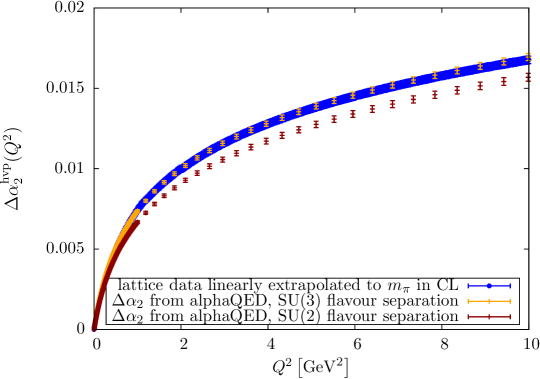
Figure 9: $N_{f}=2+1+1$ contribution to $\Delta\alpha_{2}^{\rm hvp}$ compared to the data collected in Jegerlehner:2012:Online for all quarks except the top. The lattice data are extrapolated to the physical point and to the continuum limit (CL).

Fig. 9 shows our results after combined extrapolation to the physical point and to vanishing lattice spacing compared to the results of Jegerlehner:2011mw . There, two ways of flavour separation have been implemented, one is assuming approximate $SU(3)_{f}$ and the other one $SU(2)_{f}$ symmetry neglecting OZI violating terms. Our results clearly prefer the $SU(3)_{f}$ flavour separation and thus indicate that the latter assumption is not tenable as has also been observed in Francis:2013jfa in a different context. In Fig. 9 we have multiplied the data from Jegerlehner:2012:Online with $\sin^{2}\theta_{W}(M_{Z})/\sin^{2}(\theta_{0})$ to account for the different reference values employed. As mentioned before $\sin^{2}(\theta_{0})=0.23871(9)$ and the value used by Jegerlehner is $\sin^{2}\theta_{W}(M_{Z})=0.23153(16)$ which has been measured at LEP ALEPH:2010aa . The flavour separation performed for the data set including very recent $e^{+}e^{-}$ measurements is based on isospin symmetry relations Jegerlehner:2015 and the results are much closer to the ones based on $SU(3)_{f}$ flavour separation in Fig. 9 than to the old $SU(2)_{f}$ curve. Thus, our lattice results are also compatible with the newest phenomenological analysis based on an isospin $SU(2)_{f}$ flavour separation, however, not assuming flavour non-diagonal elements to be small.

3.2.2 $\Delta^{\rm hvp}\sin^{2}\theta_{W}$

Having determined the four-flavour contributions to $\Delta\alpha_{\rm QED}^{\rm hvp}$ and $\Delta\alpha_{2}^{\rm hvp}$, it is straightforward to obtain the leading-order hadronic vacuum polarisation contribution to the running of the weak mixing angle

$$\Delta^{\rm hvp}\sin^{2}\theta_{W}(Q^{2})=\Delta\alpha_{\rm QED}^{\rm hvp}(Q^{2})-\Delta\alpha_{2}^{\rm hvp}(Q^{2})\;.$$ (27)

This is the central observable measured in various low-energy experiments in order to gain hints on beyond the SM physics. In subsection 3.2.4 below, a selection of such experiments operating at momentum transfers investigated in this work will be listed.

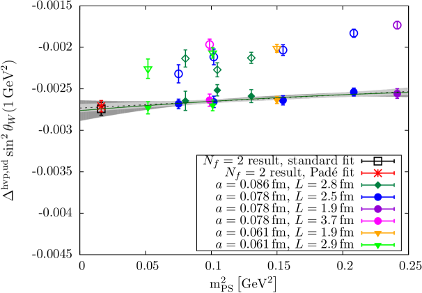
Figure 10: Light-quark contribution to $\Delta^{\rm hvp}\sin^{2}\theta_{W}$ with filled symbols representing points obtained with Eq. (11), open symbols refer to those obtained with Eqs. (2) and (21). In particular, the two-flavour results at the physical point have been computed with the standard definitions. The light grey errorband displays the uncertainty of the linear fit represented by the black dotted line wheras the dark grey errorband belongs to the quadratic fit shown as the green solid line.

The physical results for the light-quark contribution for each momentum value can again be obtained from extrapolations in the squared pion mass as shown in Fig. 10 for $Q^{2}=1\,{\rm GeV}^{2}$. In contrast to the case of $\alpha_{\rm QED}$ depicted in the left panel of Fig. 2, for the weak mixing angle combining the redefinitions according to Eq. (11) of $\alpha_{\rm QED}$ and $\alpha_{2}$ leads to lower values than obtained with the standard definitions. The common feature of the leading-order hadronic contributions of both quantities is that the values procured with the redefinitions can be already well-described by a simple linear extrapolation in the squared pion mass to the physical point yielding a result which is compatible with those of the standard analysis as well as the one from Padé approximants on the ensemble of two dynamical quarks at the physical point. The results at the physical value of the pion mass are given in table 5.

$N_{f}=2+1+1$ extrapolated	$N_{f}=2$ standard	$N_{f}=2$ $[1,1]$ Padé
-0.002717(43)	-0.002742(78)	-0.002710(68)

Table 5: Comparison of results for $\Delta^{\mathrm{hvp,ud}}\sin^{2}\theta_{W}(1\,{\rm GeV}^{2})$ at the physical point. The same analyses as indicated below table 3 have been performed.

When incorporating the heavy quarks, the chiral extrapolation is again combined with taking the continuum limit of the four-flavour result according to

$$\Delta^{\rm hvp}\sin^{2}\theta_{W}(Q^{2})(m_{\rm PS},a)=A+B~{}m_{\rm PS}^{2}+C~{}a^{2}\;.$$ (28)

The results are shown in Fig. 11. Complying with the indication from the previous subsection, we have employed the results for $\Delta\alpha_{2}^{\rm hvp}$ obtained from $SU(3)_{f}$ flavour separation in Fig. 11 together with the factor needed to take the different reference values into account. Since we do not have information on the correlation of the data in Jegerlehner:2012:Online , we have simply added the uncertainties of $\Delta\alpha_{\rm QED}^{\rm hvp}$ and $\Delta\alpha_{2}^{\rm hvp}$ in quadrature and may thus overestimate the errors of the phenomenological determination.

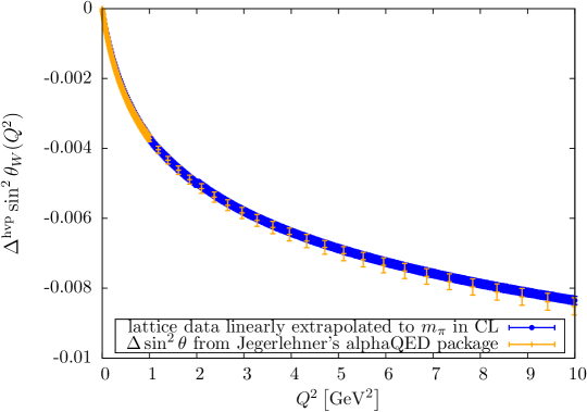
Figure 11: $N_{f}=2+1+1$ contribution to the leading-order hadronic contribution $\Delta^{\rm hvp}\sin^{2}\theta_{W}$ compared to the difference of the data collected in Jegerlehner:2012:Online .The lattice data are extrapolated to the physical point and to the continuum limit (CL).

3.2.3 Systematic uncertainties

Since the systematic uncertainties stem from the same sources as for $\Delta\alpha_{\rm QED}^{\rm hvp}$ discussed before, the relative errors are the same and only the absolute numbers differ due to the different prefactors of the renormalised vacuum polarisation function. Naturally, also the plots all look very similar. Therefore, we refrain from discussing the systematic effects separately and only summarise the general findings.

As before, due to the light quark contribution being an order of magnitude bigger than the contributions from the heavy quarks, we only need to take systematic uncertainties of this part into account. The dominant source of systematic errors is again the choice of the vacuum polarisation fit function as depicted in Fig. 12.

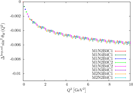
Figure 12: Light quark contribution to $\Delta^{\rm hvp}\sin^{2}\theta_{W}$ obtained from different fit functions. The standard fit is M1N2B4C1.

The only other relevant effect comes from the excited state contamination of the $\rho$-meson correlator and is shown in Fig. 13. Finite volume effects and the choice of rather heavy pion masses in the chiral extrapolation seem to be negligible in our calculation as outlined before. The only unknown systematic effect is the heavy-flavour disconnected contributions which we have neglected here.

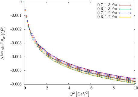
Figure 13: Light quark contribution to $\Delta^{\rm hvp}\sin^{2}\theta_{W}$ obtained with different fit ranges for the $\rho$ meson properties. The standard fit range is $[0.7\,{\rm fm},1.2\,{\rm fm}]$.

3.2.4 Final results for selected momentum values

In table 6 we collect our results for $\Delta^{\rm hvp}\sin^{2}\theta_{W}$ with statistical as well as systematic uncertainties for selected momentum values. Experiments which have measured or will measure the weak mixing angle in the respective momentum region are also indicated.

The outcome of the E158 experiment at the SLAC linear accelerator was the first successful measurement of parity violation in electron-electron (Møller) scattering Anthony:2005pm . The momentum transfer was $Q^{2}=0.026\,{\rm GeV^{2}}$. The Qweak experiment conducted at JLAB in 2012 measured parity violation in electron-proton scattering at almost exactly the same momentum transfer Armstrong:2014tna . The data is still being analysed. The predicted final uncertainty is about $5\%$ or $0.7\cdot 10^{-3}$ taking the central SM value. Another JLAB experiment performed by the PVDIS collaboration determined the weak mixing angle from parity-violating deep inelastic scattering Wang:2014bba ; Wang:2014guo which effectively means electron-quark scattering at $Q^{2}=1.085\,{\rm GeV^{2}}$ and $Q^{2}=1.901\,{\rm GeV^{2}}$. The envisioned successor of the PVDIS experiment which also measures parity violation in electron-quark scattering is the SoLID spectrometer proposed at JLAB Chen:2014psa . It can study about 20 kinematic points with $Q^{2}$ ranging from about $2\,{\rm GeV}^{2}$ to about $10\,{\rm GeV}^{2}$. Its target accuracy is $6\cdot 10^{-4}$. Our results in table 6 indicate that it will be essential to take the leading QCD corrections into account in order to deploy the whole potential of the experiment in the search for new physics beyond the SM.

$Q^{2}$ [$\rm GeV^{2}$]	this work	experiment
0.02	$-0.158\,(05)\,(08)\cdot 10^{-3}$	E158, Qweak
1.00	$-3.706\,(83)\,(127)\cdot 10^{-3}$	PVDIS
2.00	$-5.021\,(96)\,(135)\cdot 10^{-3}$	PVDIS
3.00	$-5.801\,(104)\,(135)\cdot 10^{-3}$	SoLID
4.00	$-6.398\,(102)\,(135)\cdot 10^{-3}$	SoLID
6.00	$-7.251\,(111)\,(136)\cdot 10^{-3}$	SoLID
8.00	$-7.867\,(112)\,(137)\cdot 10^{-3}$	SoLID
10.0	$-8.352\,(119)\,(138)\cdot 10^{-3}$	SoLID

Table 6: We tabulate $\Delta^{\rm hvp}\sin^{2}\theta_{W}$ for selected values of $Q^{2}$. The first error of the lattice results is statistical, the second systematic. Several low energy experiments sensitive to the respective momentum regions are indicated in the last column.

4 Summary and Outlook

Hadronic contributions to the running of electroweak parameters nowadays constitute the major uncertainties of their values even at high energies thus also limiting the precision achievable in predictions for future high-energy colliders. Here we have considered the running of $\alpha_{\rm QED}$ and of the weak mixing angle which represents one of the most important parameters of the SM and provides a sensitive probe of new physics over a large energy range.

Lattice QCD provides a most valuable tool to compute these hadronic contributions from first principles alone. As we have demonstrated in this article, lattice QCD can be used to compute to a good precision the leading-order hadronic contribution to the running of $\alpha_{\rm QED}$. In particular, we have carried out the first dynamical four-flavour calculation of the leading-order hadronic contribution to the running of the fine structure constant and the first lattice QCD calculation of the leading hadronic contribution to the shift of the weak mixing angle at energies between $0$ and $10\,{\rm GeV}^{2}$. In both cases the chiral as well as continuum extrapolations have been performed. A main effort has been undertaken to assess systematic uncertainties on a quantitative level.

For both quantities, agreement of our results with a phenomenological determination is observed with an even comparable statistical uncertainty. However, we have found that the systematic effects of the calculation still exceed the statistical errors. The dominant systematic uncertainty has been found to be the choice of fit function. Thus, methods which try to avoid fitting the vacuum polarisation are promising to reduce the overall uncertainty. A further improvement can be achieved by increasing the statistical precision which would more strongly constrain the vacuum polarisation fit. Such improvements might be accomplished by the use of the all-mode-averaging Blum:2012uh or the exact deflation Saad:1984 ; Neff:2001zr techniques.

In this article, we have provided further successful examples for the programme to determine hadronic contributions to electroweak observables from lattice QCD. The steady progress in lattice QCD with ever increasing statistical accuracy and better understanding and control of systematic uncertainties makes the lattice approach to compute these hadronic contributions very promising and gives hope that lattice results can directly be used for future low energy and collider experiments.

References

- (1) F. Jegerlehner, Electroweak effective couplings for future precision experiments, Nuovo Cim. 034C (2011) 31–40, [arXiv:1107.4683].
- (2) J. Hewett, H. Weerts, R. Brock, J. Butler, B. Casey, et al., Fundamental Physics at the Intensity Frontier, arXiv:1205.2671.
- (3) K. Hagiwara, R. Liao, A. D. Martin, D. Nomura, and T. Teubner, and re-evaluated using new precise data, J.Phys. G38 (2011) 085003, [arXiv:1105.3149].
- (4) F. Jegerlehner, The Running fine structure constant alpha(E) via the Adler function, Nucl.Phys.Proc.Suppl. 181-182 (2008) 135–140, [arXiv:0807.4206].
- (5) D. B. Renner, X. Feng, K. Jansen, and M. Petschlies, Nonperturbative QCD corrections to electroweak observables, PoS LATTICE2011 (2012) 022, [arXiv:1206.3113].
- (6) X. Feng, G. Hotzel, K. Jansen, M. Petschlies, and D. B. Renner, Leading-order hadronic contributions to and from twisted mass fermions, PoS LATTICE2012 (2012) 174, [arXiv:1211.0828].
- (7) A. Francis, G. Herdoiza, H. Horch, B. Jäger, H. B. Meyer, et al., Study of the Couplings of QED and QCD from the Adler Function, arXiv:1412.6934.
- (8) R. Baron, P. Boucaud, J. Carbonell, A. Deuzeman, V. Drach, et al., Light hadrons from lattice QCD with light (u,d), strange and charm dynamical quarks, JHEP 1006 (2010) 111, [arXiv:1004.5284].
- (9) European Twisted Mass Collaboration, R. Baron et al., Computing K and D meson masses with = 2+1+1 twisted mass lattice QCD, Comput.Phys.Commun. 182 (2011) 299–316, [arXiv:1005.2042].
- (10) F. Jegerlehner, Hadronic Contributions to Electroweak Parameter Shifts: A Detailed Analysis, Z.Phys. C32 (1986) 195.
- (11) C. Wood, S. Bennett, D. Cho, B. Masterson, J. Roberts, et al., Measurement of parity nonconservation and an anapole moment in cesium, Science 275 (1997) 1759–1763.
- (12) SLAC E158 Collaboration, P. Anthony et al., Precision measurement of the weak mixing angle in Moller scattering, Phys.Rev.Lett. 95 (2005) 081601, [hep-ex/0504049].
- (13) PVDIS Collaboration, D. Wang et al., Measurement of parity violation in electron–quark scattering, Nature 506 (2014), no. 7486 67–70.
- (14) Qweak Collaboration, D. S. Armstrong, First result from , EPJ Web Conf. 73 (2014) 07008.
- (15) MOLLER Collaboration, J. Benesch et al., The MOLLER Experiment: An Ultra-Precise Measurement of the Weak Mixing Angle Using Møller Scattering, arXiv:1411.4088.
- (16) SoLID Collaboration, J. Chen, H. Gao, T. Hemmick, Z. E. Meziani, and P. Souder, A White Paper on SoLID (Solenoidal Large Intensity Device), arXiv:1409.7741.
- (17) D. Becker, K. Gerz, S. Baunack, K. Kumar, and F. Maas, P2 - The weak charge of the proton, PoS Bormio2013 (2013) 024.
- (18) K. Kumar, S. Mantry, W. Marciano, and P. Souder, Low Energy Measurements of the Weak Mixing Angle, Ann.Rev.Nucl.Part.Sci. 63 (2013) 237–267, [arXiv:1302.6263].
- (19) T. Aoyama, M. Hayakawa, T. Kinoshita, and M. Nio, Tenth-Order QED Contribution to the Electron g-2 and an Improved Value of the Fine Structure Constant, Phys.Rev.Lett. 109 (2012) 111807, [arXiv:1205.5368].
- (20) F. Jegerlehner and A. Nyffeler, The Muon g-2, Phys. Rept. 477 (2009) 1–110, [0902.3360].
- (21) ETM Collaboration, R. Baron et al., Light hadrons from Nf=2+1+1 dynamical twisted mass fermions, PoS LATTICE2010 (2010) 123, [arXiv:1101.0518].
- (22) F. Burger, X. Feng, G. Hotzel, K. Jansen, M. Petschlies, and D. B. Renner, Four-Flavour Leading-Order Hadronic Contribution To The Muon Anomalous Magnetic Moment, JHEP 1402 (2014) 099, [arXiv:1308.4327].
- (23) F. Burger, G. Hotzel, K. Jansen, and M. Petschlies, Leading-order hadronic contributions to the electron and tau anomalous magnetic moments, arXiv:1501.05110.
- (24) A. Abdel-Rehim, P. Boucaud, N. Carrasco, A. Deuzeman, P. Dimopoulos, et al., A first look at maximally twisted mass lattice QCD calculations at the physical point, PoS LATTICE2013 (2013) 264, [arXiv:1311.4522].
- (25) A. Abdel-Rehim, C. Alexandrou, P. Dimopoulos, R. Frezzotti, K. Jansen, et al., Progress in Simulations with Twisted Mass Fermions at the Physical Point, PoS LATTICE2014 (2014) 119, [arXiv:1411.6842].
- (26) ETM Collaboration, A. Abdel-Rehim et al., Simulating QCD at the Physical Point with Wilson Twisted Mass Fermions at Maximal Twist, arXiv:1507.05068.
- (27) G. Ecker, J. Gasser, A. Pich, and E. de Rafael, The Role of Resonances in Chiral Perturbation Theory, Nucl.Phys. B321 (1989) 311.
- (28) C. Aubin and T. Blum, Calculating the hadronic vacuum polarization and leading hadronic contribution to the muon anomalous magnetic moment with improved staggered quarks, Phys. Rev. D75 (2007) 114502, [hep-lat/0608011].
- (29) Particle Data Group Collaboration, K. Olive et al., Review of Particle Physics, Chin.Phys. C38 (2014) 090001.
- (30) X. Feng, K. Jansen, M. Petschlies, and D. B. Renner, Two-flavor QCD correction to lepton magnetic moments at leading-order in the electromagnetic coupling, Phys.Rev.Lett. 107 (2011) 081802, [arXiv:1103.4818].
- (31) C. Aubin, T. Blum, M. Golterman, and S. Peris, Model-independent parametrization of the hadronic vacuum polarization and g-2 for the muon on the lattice, Phys.Rev. D86 (2012) 054509, [arXiv:1205.3695].
- (32) F. Burger, G. Hotzel, K. Jansen, and M. Petschlies, The hadronic vacuum polarization and automatic improvement for twisted mass fermions, JHEP 1503 (2015) 073, [arXiv:1412.0546].
- (33) F. Jegerlehner, alphaQED, http://www-com.physik.hu-berlin.de/ fjeger/software.html (April, 2012).
- (34) F. Jegerelehner private communication.
- (35) X. Feng, S. Hashimoto, G. Hotzel, K. Jansen, M. Petschlies, et al., Computing the hadronic vacuum polarization function by analytic continuation, Phys.Rev. D88 (2013) 034505, [arXiv:1305.5878].
- (36) A. Francis, B. Jäger, H. B. Meyer, and H. Wittig, A new representation of the Adler function for lattice QCD, Phys.Rev. D88 (2013) 054502, [arXiv:1306.2532].
- (37) G. de Divitiis, R. Petronzio, and N. Tantalo, On the extraction of zero momentum form factors on the lattice, Phys.Lett. B718 (2012) 589–596, [arXiv:1208.5914].
- (38) F. Jegerlehner, Vector Boson Parameters: Scheme Dependence and Theoretical Uncertainties, Z.Phys. C32 (1986) 425.
- (39) V. Dzuba, J. Berengut, V. Flambaum, and B. Roberts, Revisiting parity non-conservation in cesium, Phys.Rev.Lett. 109 (2012) 203003, [arXiv:1207.5864].
- (40) J. Erler and M. J. Ramsey-Musolf, The Weak mixing angle at low energies, Phys.Rev. D72 (2005) 073003, [hep-ph/0409169].
- (41) ATLAS Collaboration, G. Aad et al., Observation of a new particle in the search for the Standard Model Higgs boson with the ATLAS detector at the LHC, Phys.Lett. B716 (2012) 1–29, [arXiv:1207.7214].
- (42) CMS Collaboration, S. Chatrchyan et al., Observation of a new boson at a mass of 125 GeV with the CMS experiment at the LHC, Phys.Lett. B716 (2012) 30–61, [arXiv:1207.7235].
- (43) W. J. Marciano, Spin and precision electroweak physics, Spin structure in high energy processes: Proceedings (1993) 35–56.
- (44) F. Jegerlehner, Renormalizing the standard model, Conf.Proc. C900603 (1990) 476–590.
- (45) W. Wetzel, The Hadronic Contribution to the and Mass, Z.Phys. C11 (1981) 117.
- (46) W. Marciano and A. Sirlin, On Some General Properties of the O(alpha) Corrections to Parity Violation in Atoms, Phys.Rev. D29 (1984) 75.
- (47) A. Francis, G. von Hippel, H. B. Meyer, and F. Jegerlehner, Vector correlator and scale determination in lattice QCD, PoS LATTICE2013 (2013) 320, [arXiv:1312.0035].
- (48) ALEPH Collaboration, CDF Collaboration, D0 Collaboration, DELPHI Collaboration, L3 Collaboration, OPAL Collaboration, SLD Collaboration, LEP Electroweak Working Group, Tevatron Electroweak Working Group, SLD Electroweak and Heavy Flavour Groups Collaboration, Precision Electroweak Measurements and Constraints on the Standard Model, arXiv:1012.2367.
- (49) D. Wang, K. Pan, R. Subedi, Z. Ahmed, K. Allada, et al., Measurement of Parity-Violating Asymmetry in Electron-Deuteron Inelastic Scattering, arXiv:1411.3200.
- (50) T. Blum, T. Izubuchi, and E. Shintani, New class of variance-reduction techniques using lattice symmetries, Phys.Rev. D88 (2013), no. 9 094503, [arXiv:1208.4349].
- (51) Y. Saad, Tchebyshev Acceleration Techniques for Solving Nonsymmetric Eigenvalue Problems, Math. Comp. 42 (1984) 567–588.
- (52) H. Neff, N. Eicker, T. Lippert, J. W. Negele, and K. Schilling, On the low fermionic eigenmode dominance in QCD on the lattice, Phys.Rev. D64 (2001) 114509, [hep-lat/0106016].