Spin Model of O₂-based Magnet in a Nanoporous Metal Complex

Abstract

Inelastic neutron scattering experiments are performed on a nanoporous metal complex Cu-Trans-1,4-Cyclohexanedicarboxylic Acid (Cu-CHD) adsorbing O₂ molecules to identify the spin model of the O₂-based magnet realized in the host complex. It is found that the magnetic excitations of Cu-CHDs adsorbing low- and high-concentration O₂ molecules are explained by different spin models, the former by spin dimers and the latter by spin trimers. By using the obtained parameters and also by assuming that the levels of the higher energy states are reduced because of the non-negligible spin dependence of the molecular potential of oxygen, the magnetization curves are explained in quantitative level.

I Introduction

Natural oxygen, the second abundant constituent in the air, is a magnet having spin $S$=l induced by a couple of ${\pi}_{g}$ electrons. The oxygen molecules are condensed and crystalized at 54 K by van-der Waals interaction. The solid oxygen realized at the low temperatures include ${\alpha}$ phase with monoclinic $C2/m$ at $T\leq 23$ K, ${\beta}$ phase with hexagonal $R\bar{3}m$ at $23~{}{\rm K}<T\leq 43$ K, and ${\gamma}$ phase with cubic $Pm3n$ at $43~{}{\rm K}<T\leq 54$ K.Uyeda ; Freimana Since the magnetic system is phenomenologically coupled to the lattice system thorough magneto-elastic coupling, the successive phase transition is magneto-structural transition accompanied by the change of the spin Hamiltonian. Magnetic susceptibility measurements suggested that quasi-two-dimensional spin system in the $\alpha$ phase, triangular spin system in the $\beta$ phase, and one-dimensional spin system in the $\gamma$ phase were realized.Uyeda Applying pressure induces more phases including metal,Desgreniers superconductivity,Shimizu , and an insulating magnetically ordered phases.Goncharenko The variety of the phases suggests that the energy scales of the coupling among multi-degrees of freedom, i.e., lattice, spin, and orbital, are close to each other in the soft solid crystalized by Van der Waals interaction. Indeed the molecular potential between a pair of O₂ molecules is strongly dependent on the spin state, which means that the geometrical configuration of the O₂ molecules and the spin state are closely correlated.Hemert ; Wormer ; Bussery ; Bussery94 ; Nozawa ; Obata To manipulate the oxygen molecule O₂ and to artificially synthesize a novel type of O₂-based magnet is, therefore, the challenge in the new field of magnetism.

Pioneering work is found in the adsorbed O₂ on the surface of graphite, where triangular lattice of O₂ is realized.McTague ; Murakami Combination of the magnetic susceptibility and neutron diffraction measurements reveals the magnetically ordered state at low temperatures. Another root for the O₂-based magnet is to utilize nano-materials such as microporous metal complexes,Kitagawa ; Takamizawa ; Takamizawa2 ; Kondo ; Mori ; Masuda nanoporous silica,Wallacher ; AckermannEPL or carbon nanotubes.Hagiwara The adsorbed molecules staying at the minimum of the Van der Waals potential in the nanopore form a supercrystal, leading to the realization of the O₂-based magnet.

We focus our attention on a metal complex having one-dimensional nanopores, Cu-Trans-1,4-Cyclohexanedicarboxylic Acid Cu₂(OOC-C₆H₄-COO) abbreviated as Cu-CHD.Mori The adsorbed O₂ molecules form dimer-like structure in the nanopores.Hori Indeed, the magnetic susceptibility of Cu-CHD adsorbing 0.18 mole of O₂ per half of formula unit showed a rapid decrease with the decrease of the temperature, which is consistent with a spin dimer model. It was, however, explained not by $S$=1 spin dimer but rather by $S$ = 1/2 spin dimer. To explain the unusual bulk property, the spin-dependent Van der Waals potentialHemert ; Wormer ; Bussery ; Bussery94 was discussed, and the anomalous energy spectrum was proposed.Hori The precise energy scheme is to be directly revealed by a spectroscopic technique.

The magnetic susceptibility of Cu-CHD adsorbing high concentration of O₂ molecules showed qualitatively different behavior from that of the low concentration one. Curie-Weiss like behavior was enhanced in the low $T$ region.Mori The result suggested that the spin model and the corresponding energy scheme can be tuned by the concentration of the O₂ molecules in the O₂-based magnet. The detailed model is to be experimentally identified.

In the present study we carried out inelastic neutron scattering (INS) experiments at low temperatures in order to observe the low-energy excitations and to clarify the spin model of the O₂-based magnet realized in Cu-CHD. We found that the magnetic excitation of Cu-CHD adsorbing less O₂ is explained by a spin-dimers model of which the exchange constants are normally distributed. In contrast, that of Cu-CHD adsorbing more O₂ is explained by a spin-trimers model with the distributed exchange constants. It was found that the spin model is tuned by the concentration of O₂ in this system. Based on the spin models with the conclusive parameters determined by INS experiments and by introducing the reduction of the energy levels of higher states, we quantitatively explained the magnetization curves. The effect of the spin-dependent Van der Waals potential to the anomalous energy scheme is experimentally confirmed.

II Experimental details

Polycrystalline Cu-CHD was synthesized in methanol solution. The details are described elsewhere.Inoue The total mass was 5.93 g. Since Cu-CHD includes many hydrogen atoms that have large incoherent neutron scattering cross sections, we paid special attention to extract the net contribution of the adsorbed oxygen molecules. The first step was to prepare the bare Cu-CHD sample in which any type of guest molecules including H₂O, N₂, O₂, etc., were eliminated. The second step was to measure the INS spectrum of the bare Cu-CHD sample as background data. The third step was to prepare the oxygen adsorbed Cu-CHD sample. Here we used exactly the same sample that was used for the background measurement in the second step. The forth step was to measure the INS spectrum of the oxygen adsorbed Cu-CHD. Ideally the net contribution of the adsorbed oxygen can be extracted by subtracting the INS spectrum in the second step from that in the forth step. In reality we found additional intensity that increased with the increase of the wave number transfer $Q$ even after the background subtraction process. In addition we found flat intensity that was independent both on $Q$ and the energy transfer $\hbar\omega$. During the analyses on the data after background subtraction, therefore, we used additional background of which the form was $A({\hbar}{\omega})Q^{2}+B$. Here $A({\hbar}{\omega})$ and $B$ were free parameters. We could not identify the origin of the additional background, even though we could make some speculations; $A({\hbar}{\omega})$ term would be from the deformation of the host compound after the oxygen adsorption, and $B$ term would be from the difference of white background such as electronic noise between before and after the oxygen adsorption.

The procedure of preparing the bare Cu-CHD is as follows. The Cu-CHD sample in the Aluminum made container was warmed at about 105 ^∘C and was evacuated by a vacuum pump with monitoring the pressure. We used the gas evacuation/introduction system described in Fig. 2 in Ref.Masuda, We waited until the pressure reached a few Pa, which is the capacity limit of the vacuum pump, and we confirmed that the Cu-CHD sample had discharged all the molecules. We, then, seal the container by closing a V1 valve in Fig. 2 in Ref.Masuda, , put the sample in a liquid helium cryostat, cool the temperature down to 4.5 K, and collected INS spectrum of the bare Cu-CHD. After the background measurement we set the temperature of the bare Cu-CHD at 110 K and introduced O₂ gas in the nanopore by using a buffer container of which the capacities were known. The pressure of the gas was kept below 8$\times$10⁴ Pa. The volume of the introduced oxygen was estimated by the capacity of the buffer container and the pressure of the O₂ gas inside the container. After the O₂ introduction procedure the sample container was sealed, and was cooled down to 4.5 K. All measurements were carried out at $T$=4.5 K. We prepared two samples that adsorbed different amount of O₂ in order to examine the O₂ concentration dependence of the spin model realized in the nanopores. Exactly the same polycrystalline Cu-CHD was used as the host compound for both samples. In prior to the preparation of each sample we discharged the gas in the nanopore at 105 ^∘C according to the procedure described above. The O₂ mole ratios sealed in the sample container were O₂/(Cu atom)=0.3${\pm}0.07$ and 2.0${\pm}0.4$, which are labeled as 0.3O₂-(Cu-CHD) and 2.0O₂-(Cu-CHD), respectively.

Neutron scattering experiment was carried out using the cold neutron chopper spectrometer AMATERAS installed at J-PARC.Nakajima ; Inamura The initial neutron energies $E_{i}$=3.135 meV and $E_{i}$=7.743 meV were used, and their energy resolutions are about 0.15 and 0.45 meV at the elastic position.

III Results

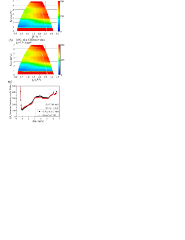
Figure 1: (Color online) (a) Contour map of the raw neutron spectrum bare-(Cu-CHD) by using $E_{i}$=7.743 meV. (b) Contour map of the raw neutron spectrum 0.3O₂-(Cu-CHD) by using $E_{i}$=7.743 meV. (c) One-dimensional energy cut obtained by integrating the intensity in the range of $1.2~{}{\rm\AA}^{-1}\leq Q\leq 1.4~{}{\rm\AA}^{-1}$ for raw data of 0.3O₂-(Cu-CHD) and bare Cu-CHD.

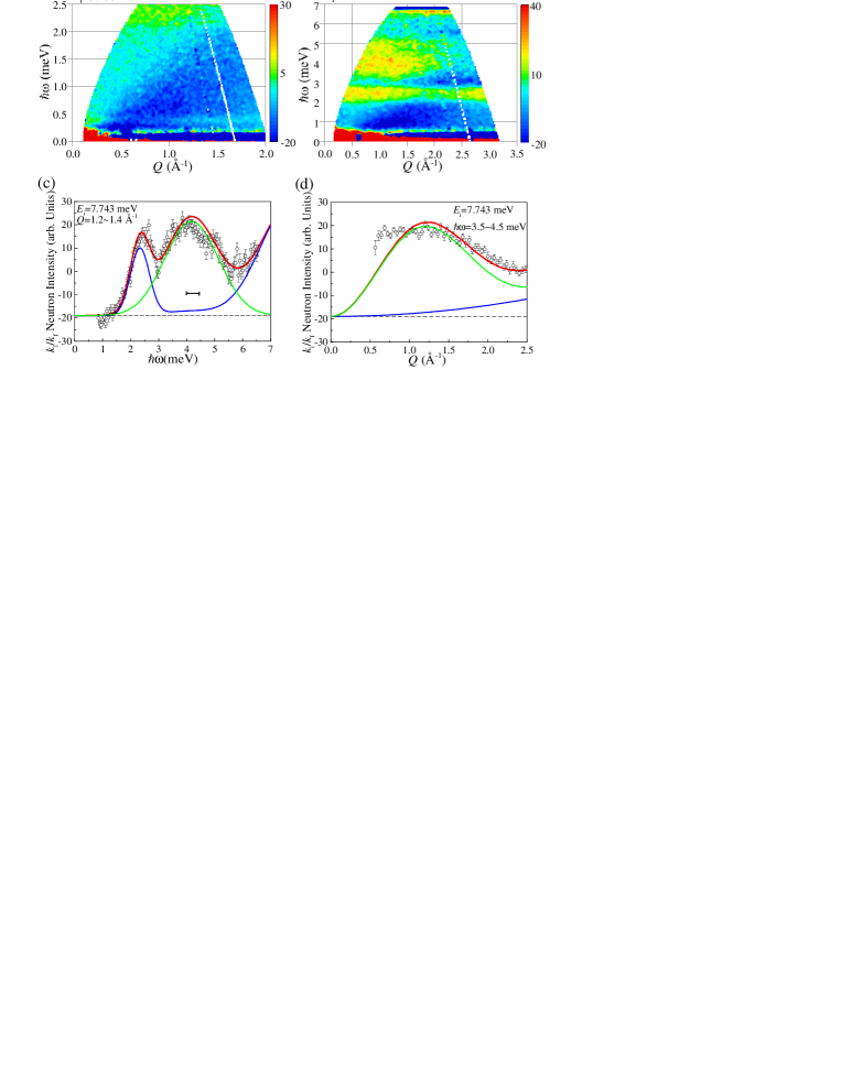
Figure 2: (Color online) (a,b) Contour map of the neutron spectrum of 0.3O₂-(Cu-CHD) after the background subtraction by using (a) $E_{i}$=3.135 meV and (b) $E_{i}$=7.743 meV. (c,d) Neutron intensity for 0.3O₂-(Cu-CHD) after the background subtraction by using $E_{i}$=7.743 meV. The green curve is the neutron cross section of a group of spin dimers having distributed $J$. The blue curve is the additional background having $Q$ dependence. The red curve is the sum of green and blue curves. The dashed line shows the additional flat background. (c) One-dimensional energy cut obtained by integrating intensity in the range of $1.2~{}{\rm\AA}^{-1}\leq Q\leq 1.4~{}{\rm\AA}^{-1}$. The energy resolution is shown by the horizontal bar. (d) One-dimensional $Q$ cut obtained by integrating intensity in the range of $3.5~{}{\rm meV}\leq E\leq 4.5~{}{\rm meV}$.

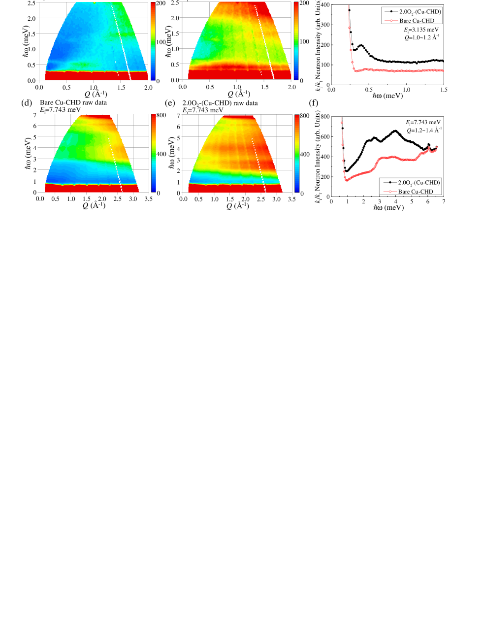
Figure 3: (color online) (a,b) Contour map of the raw neutron spectrum of (a) bare Cu-CHD and (b) 2.0O₂-(Cu-CHD) by using $E_{i}$=3.135 meV. (c) One-dimensional energy cut in the low-energy region obtained by integrating intensity in the range of $1.0~{}{\rm\AA}^{-1}\leq Q\leq 1.2~{}{\rm\AA}^{-1}$ for raw 2.0O₂-(Cu-CHD) and bare Cu-CHD by using $E_{i}$=3.135 meV. (d,e) Contour map of the raw neutron spectrum of (d) bare Cu-CHD and (e) 2.0O₂-(Cu-CHD) by using $E_{i}$=7.743 meV. (f) One-dimensional energy cut in the high-energy region obtained by integrating intensity in the range of $1.2~{}{\rm\AA}^{-1}\leq Q\leq 1.4~{}{\rm\AA}^{-1}$ for raw 2.0O₂-(Cu-CHD) and bare Cu-CHD by using $E_{i}$=7.743 meV.

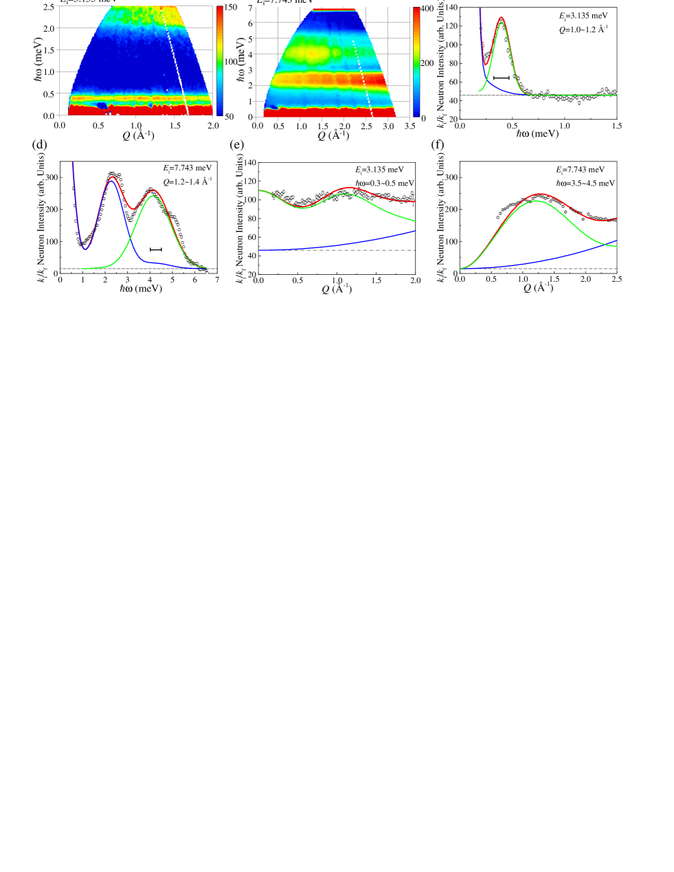
Figure 4: (color online) Neutron intensity for 2.0O₂-(Cu-CHD) after the background subtraction. The green curve is the magnetic excitation, the blue curve is the additional background having $Q$ dependence, and the red curve is the sum of green and blue curves. The dashed line shows the background. (a) One-dimensional energy cut in the low-energy region obtained by integrating intensity in the range of $1.0~{}{\rm\AA}^{-1}\leq Q\leq 1.2~{}{\rm\AA}^{-1}$. The energy resolution is shown by the horizontal bar. (b) One-dimensional energy cut in the high-energy region obtained by integrating intensity in the range of $1.2~{}{\rm\AA}^{-1}\leq Q\leq 1.4~{}{\rm\AA}^{-1}$. (c) One-dimensional $Q$ cut obtained by integrating intensity in the range of $0.3~{}{\rm meV}\leq E\leq 0.5~{}{\rm meV}$. The energy resolution is shown by the horizontal bar. (d) One-dimensional $Q$ cut obtained by integrating intensity in the range of $3.5~{}{\rm meV}\leq E\leq 4.5~{}{\rm meV}$.

Figures 1(a) and (b) show the raw inelastic neutron scattering (INS) spectra of bare Cu-CHD and 0.3O₂-(Cu-CHD), respectively. The initial energy $E_{i}$ is 7.743 meV. Strong incoherent scattering from hydrogen atoms and/or functional groups were observed in the wide region in the energy transfer ($\hbar\omega$) - wave number transfer ($Q$) space in both panels. Figure 1(c) shows typical one-dimensional (1D) energy cut obtained by integrating the intensity in the range of $1.2~{}{\rm\AA}^{-1}\leq Q\leq 1.4~{}{\rm\AA}^{-1}$ for the raw spectrum of 0.3O₂-(Cu-CHD) and that of the bare Cu-CHD. Statistically meaningful increases are observed at about 2.5 meV and 4 meV in 0.3O₂-(Cu-CHD). The enhancement of the intensity is due to the additional scattering of the adsorbed oxygen molecules. The decrease of the intensity is observed at about 1 meV in Fig. 1(b). As we described in the Section II the INS spectrum of the bare Cu-CHD is regarded as background, but its intensity is comparable to the 0.3O₂-(Cu-CHD) because of the large incoherent scattering from the hydrogen atoms included. Even though the careful background measurement, the background has rather larger intensity than 0.3O₂-(Cu-CHD), of which the origin would be unavoidable artifacts.

Figure 2(a) shows the INS spectrum of 0.3O₂-(Cu-CHD) after the background subtraction in the low-energy region for the data set of $E_{i}$=3.135 meV. The absence of excitation at $\hbar\omega\lesssim 2$ meV is confirmed in the experimental error. Figure 2(b) shows the INS spectrum of 0.3O₂-(Cu-CHD) in the high energy region for the data set of $E_{i}$=7.743 meV after the background subtraction. The dispersionless excitations are observed at $\hbar\omega$$\simeq$2.4 meV and 4 meV. These two excitations are also probed as two peaks in the 1D-energy cut after the background subtraction shown in Fig. 2(c).

To examine the $Q$-dependence of the excitation at $\hbar\omega$$\simeq$4 meV, the 1D-$Q$ cut obtained by integrating the intensity in the range of $3.5~{}{\rm meV}\leq\hbar\omega\leq 4.5~{}{\rm meV}$ is shown in Fig. 2(d). The intensity of the excitation has a kink at about 1.2 Å^-1 and it decreases with increasing $Q$. The dispersionless behavior means that the origin of the excitation is a cluster. The suppressed intensity at large $Q$ means that the excitation is dominated by a magnetic scattering. The excitation induced by the oxygen adsorption is, therefore, the magnetic one from some types of the O₂ molecules cluster. The kink at finite $Q$ means that the spin correlation is antiferromagnetic, and the maximum $Q$ exhibits the inversed length-scale of the intra-cluster distance. As for the excitation at $\hbar\omega$$\simeq$2.4 meV in Fig. 2(b), the intensity shows monotonic decrease with the increase of $Q$ in the range of $Q\lesssim 2.2{\rm\AA}^{-1}$ and, then, it increases in the range of $2.2{\rm\AA}^{-1}\lesssim Q$. We considered that this excitation is not intrinsically magnetic one, which will be discussed later.

Raw INS spectra of the bare Cu-CHD and the 2.0O₂-(Cu-CHD) with $E_{i}=3.135$ meV are shown in Fig. 3 (a) and (b), respectively. A flat excitation at $\hbar\omega\sim 0.4$ meV is newly observed in the 2.0O₂-(Cu-CHD) in addition to smeared intensities in wide $\hbar\omega$ - $Q$ space. 1D-energy cuts of the 2.0O₂-(Cu-CHD) and the bare Cu-CHD in the integration range of 1.0 Å${}^{-1}\leq Q\leq$ 1.2 Å^-1 is shown in Fig. 3 (c). Peak structure at 0.4 meV is clearly observed. Raw INS spectra of the bare Cu-CHD and the 2.0O₂-(Cu-CHD) with $E_{i}=7.743$ meV are shown in Fig. 3(d) and (e), respectively. The spectrum in Fig. 3(d) is the same data as shown in Fig. 1(a) but the intensity scale is different. Broad excitations at 3 meV $\lesssim\hbar\omega\lesssim$ 5 meV in low $Q$ region are newly observed in 2.0O₂-(Cu-CHD). The 1D-energy cuts for $E_{i}$ = 7.743 meV is shown in Fig. 3 (f). The Cu-CHD adsorbing more O₂ molecules exhibits the large enhancement of the neutron intensity compared to those of 0.3O₂-(Cu-CHD).

The INS spectrum of 2.0O₂-(Cu-CHD) by using the $E_{i}$=3.135 meV after the background subtraction is shown in Fig. 4(a). The dispersionless excitation is observed at $E$$\simeq$0.4 meV. The 1D-energy cut in Fig. 4(c) exhibits that the energy width of the excitation is almost the resolution limited. The INS spectra of 2.0O₂-(Cu-CHD) by using the $E_{i}$=7.743 meV after the background subtraction is shown in Fig. 4(b). The dispersionless excitations are observed at $\hbar\omega$$\simeq$2.4 meV and 4 meV. These excitations have the broad width as shown by the 1D-energy cut in Fig. 4(d).

In order to examine the $Q$-dependence of the excitation at 0.4 meV, the 1D-$Q$ cut obtained by the integration in the range of $0.3~{}{\rm meV}\leq E\leq 0.5~{}{\rm meV}$ is shown in Fig. 4(e). The dispersionless excitation has broad peak at $Q$=1.2 Å^-1 of which the wave number corresponds to the distance between O₂ molecules. This excitation is not clearly observed in 0.3O₂-(Cu-CHD). The energy of the excitation is quite close to the anisotropy energy of the natural oxygen in the gas phase reported as 0.5 meV.Kimura This suggested that the excitation is due to the single-ion-anisotropy of the adsorbed oxygen molecules.

The 1D-$Q$ cut for the excitation at 4 meV is obtained by the integration range of $3.5~{}{\rm meV}\leq E\leq 4.5{\rm meV}$ in Fig. 4(f). The excitation has the peaks at about 1.2 Å^-1 and the intensities decrease with increasing $Q$. The qualitative behavior is the same as that of 0.3O₂-(Cu-CHD), meaning that the origin of the excitation is a cluster of O₂ molecules.

The excitation at $\hbar\omega$$\simeq$2.4 meV exhibits stronger intensity at high $Q$. This means that its origin is nuclear lattice or cluster rather than magnetic one. We will exclude the excitation in the analysis section. Similarly we consider that the excitation at $\hbar\omega$$\simeq$2.4 meV in 0.3O₂-(Cu-CHD) would have nuclear origin.

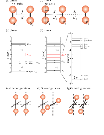
Figure 5: (Color online) (a) O₂ configuration used in the calculation of the dimer model. (b) O₂ configuration used in the calculation of trimer model. (c) Black lines show energy levels calculated by conventional spin Hamiltonian of $S$=1 dimer model. Red lines show the reduced energy levels to reproduce the magnetization. (d) Black lines show energy levels calculated by conventional spin Hamiltonian of $S$=1 trimer model. Red lines show the reduced energy levels to reproduce the magnetization. (e) O₂ dimer in H-configuration. (f) O₂ dimer in X-configuration. (g) O₂ dimer in S-configuration.

IV Analyses

Combination of synchrotron x-ray diffraction and maximum entropy method/Rietveld analysis revealed that the adsorbed O₂ molecules form dimers in the nanopore.Hori We, therefore, start our analysis on the magnetic excitation at $E$$\simeq$4 meV in 0.3O₂-(Cu-CHD) from the $S=1$ spin-dimer model shown in Fig. 5(a). We assume that the molecular axes of two O₂ molecules are parallel. The distance between the oxygen molecules, $d$, is fixed with the reported value 3.22 Å.Hori The magnetic anisotropy axis is along the molecular axis, Tinkham which is defined as $z$ - axis. The spin Hamiltonian is

$$\mathcal{H}_{dimer} = J\mbox{\boldmath$S_{1}$}\cdot\mbox{\boldmath$S_{2}$}+D\sum_{l}\left(S_{l}^{z}\right)^{2}.$$ (1)

The neutron cross section within the Born approximation Squire is calculated by the diagonalization of the Hamiltonian. The powder average was, then, performed to compare the calculation with the experiment. We used the magnetic form factor $F(\mbox{\boldmath$Q$})=\int^{\infty}_{0}\int^{\pi}_{0}drd\theta r^{4}\mbox{sin}^{3}\theta e^{-2br^{2}}[\mbox{cosh}(2bR_{0}\mbox{cos}\theta)-1]e^{iQr\mbox{cos}(\theta-\beta)}$ as described in Ref. formfactor, . Here, we used the internuclear distance $R$₀=1.21 Å and a constant $b$=4.1 Å^-2. $\beta$ is the angle between the molecular axis and the scattering vector.

Since the calculated neutron cross section of a spin cluster is a dispersionless delta function, the peak width of the excitation should be resolution limited. In contrast the excitation, which is guided by the green curve in Fig. 1 (e), exhibits the larger width than that of the experimental resolution. The shape of the excitation is rather symmetric, and the asymmetry due to Van-Hove singularity is not observed. This suggests that the finite width is ascribed not to the powder-averaged dispersion due to an interdimer coupling but to the distribution of the intradimer exchange constants of isolated dimers. We consider that multiple minima for O₂ molecules are there inside the nanopore of Cu-CHD, leading to randomness of the configuration of O₂ dimer. Then the spin system is considered as a group of dimers having different $J$s. We assume that the distribution of the $J$s is Gaussian function. The free parameters for the fitting to the data are, thus, the mean value of the exchange interaction redefined as $J$, and the standard deviation of the distribution $\sigma$. In this analysis, the uniaxial anisotropy $D$ is not very important because the magnitude of $\sigma$ is much larger than that of $D$. We fixed $D$ = 0.41 meV that is independently determined in the analysis of 2.0O₂-(Cu-CHD) which will be explained later. We also consider the additional background with the form of $A(\hbar\omega)Q^{2}+B$.

Table 1: Parameteres obtained for the 0.3O₂-(Cu-CHD) sample from INS experiment (upper) and those for the 0.22O₂-(Cu-CHD) sample from magnetization measurement (lower).

	$J$ (meV)	$d$ (Å)	$\sigma$ (meV)	$D$ (meV)	$N$(%)	${\Delta}E$
INS	4.15	3.22	2.16	0.41	-	-
$M$ Dimer	4.15	-	1.77	0.41	90	1.15J
$M$ Monomer	-	-	-	0.41	10	-

For the fitting we use the data of one-dimensional energy cut in Fig. 2(c) and one-dimensional $Q$ cut in Fig. 2(d). In the first step we fit the one-dimensional energy cut by three Gaussians to obtain the peak energy and the energy width. We introduce the additional background with the phonon-like form i.e., $A_{n}{\exp}[-(({\hbar}{\omega}-{\hbar}{\omega}_{n})/\sqrt{2}{\Delta}_{n})^{2}]Q^{2}$ ($n=1,2,3$) and the additional flat background $B$. Here $\hbar{\omega}_{n}$ are the peak energies obtained in the first step. In the second step we fit the sum of the neutron cross section of the group of dimers and the additional background, $\sum_{n}(A_{n}{\exp}[-(({\hbar}{\omega}-{\hbar}{\omega}_{n})/\sqrt{2}{\Delta}_{n})^{2}]Q^{2})+B$ to the data of one-dimensional $Q$ cut and one-dimensional energy cut. Fitting parameters are $J$, $\sigma$, scale factor for the cross section of group dimers, $A_{n}(n=1,2,3)$, and $B$.

The calculated cross sections with the parameters summarized in Table I are shown by by the green solid curves in Figs. 2(c) and 2(d). The blue curves are the additional background, and the red solid curves are the sum of green and blue curves. The data are reasonably reproduced by the calculation, meaning that the magnetic excitation of the 0.3O₂-(Cu-CHD) at $T$ = 4.5 K is explained by the spin dimers with normally distributed exchange constants.

The eigenenergies of a single dimer calculated by using the parameters of $J$ and $D$ in Table I are shown by the black lines in Fig. 5(c). The ground state, $E_{G}$, is nonmagnetic singlet. The first group of the excited states, $E_{1st}$, is composed of nearly triplet states with $S$=1, which are lifted by the single-ion anisostopy $D$. The second group, $E_{2nd}$, is composed of nearly quintet states with $S$=2. The transition between $E_{G}$ and $E_{1st}$ is probed as the excitation at $\hbar\omega=4$ meV in the INS spectrum.

In the INS spectrum in 2.0O₂-(Cu-CHD) we observed a couple of magnetic excitations at $E$$\simeq$0.4 meV and 4 meV. The latter excitation looks similar to that observed in 0.3O₂-(Cu-CHD), but the simple dimer model does not explain the 0.4 meV excitation. In fact the triplet state is the ground state in case that the cluster is composed of the odd number of Heisenberg spins, and, therefore, the transition between the triplet states lifted by the single-ion anisotropy $D$ can be probed as the low energy excitation. In the monomer case, the cross section decreases monotonically with increasing $Q$ because it depends solely on the magnetic form factor. In Fig. 3 (g) the cross section exhibits a peak at $Q$$\simeq$1.2 Å^-1, meaning that the cluster is composed of the multiple spins. We, thus, consider the trimer of O₂ molecules shown in Fig. 5(b). We assume that the molecular axes are parallel. The trimer has two different inter-molecular lengths, $d_{1}$ and $d_{2}$, and correspondingly two different exchange constants, $J_{1}$ and $J_{2}$. The spin Hamiltonian of a trimer is, thus,

$$\mathcal{H}_{trimer} = J_{1}\mbox{\boldmath$S_{1}$}\cdot\mbox{\boldmath$S_{2}$}+J_{2}\mbox{\boldmath$S_{2}$}\cdot\mbox{\boldmath$S_{3}$}+D\sum_{l}\left(S_{l}^{z}\right)^{2}.$$ (2)

The neutron cross section is calculated by the diagonalization of the Hamiltonian. The free parameters are the exchange interactions $J_{1}$, $J_{2}$, the uniaxial anisotropy $D$, and one of the inter-molecular distances $d_{2}$. Another distance, $d_{1}$, is fixed to 3.22 Å. Hori We assume that the width of the magnetic excitation at $E$$\simeq$4 meV is due to the normal distribution of the exchange constant $J_{1}$. We define that the standard deviation $\sigma_{1}$ of the distribution, and redefine the mean value of the exchange constants as $J_{1}$. Both of them are the free parameters for the calculation. The standard deviation $\sigma_{2}$ of $J_{2}$ is fixed to 0. The additional background is also considered in a similar way to the analysis in 0.3O₂-(Cu-CHD).

The calculated cross sections are shown by the solid curves in Figs. 3(e)-3(h), and the obtained parameters are shown in Table II. The green curve is the magnetic excitation, the blue curve is additional background, and the red curve is the sum of green and blue curves. The data is reasonably reproduced by the spin trimers of which the main exchange constants are normally distributed. We note that the ratio of the peak intensity at $Q$$\simeq$1.2 Å^-1 to the amplitude of the intensity modulation in Fig. 3 (g) is tuned by the ratio of $J_{1}$ to $J_{2}$. The value of $d_{2}$ is larger than that of $d_{1}$, and the value of $J_{2}$ is much smaller than that of $J_{1}$. This means that the O₂ trimers in the high oxygen concentration sample 2.0O₂-(Cu-CHD) are regarded as the O₂ dimers weakly coupled to O₂ monomers.

The energy level of a single trimer calculated by the obtained parameters and the mean exchange constant $J_{1}$ are shown by the black lines in Fig. 5(d). The eigenstates of the trimer model are separated into the three groups. The group having the low energy, $E_{G}$, is $S$ = 1 states lifted by the single-ion anisotropy $D$. They are composed of 3 states and the ground state is $S_{z}$=0. The first group of the excited states, $E_{1st}$, is composed of 9 states, and the second group, $E_{2nd}$, is composed of 15 states. The excitation at $E$$\simeq$0.4 meV corresponds to the transitions among the $E_{G}$ states. The excitation at $E$$\simeq$4 meV corresponds to the transitions between $E_{G}$ states and $E_{1st}$ states.

The $Q$ dependence of the excitation at 4 meV in 2.0O₂-(Cu-CHD) is similar to that in 0.3O₂-(Cu-CHD), since they are physically quite similar. If $J_{2}$ is zero and the system is composed of isolated dimers and monomers, the transition between $E_{G}$ and $E_{1st}$ in the system is exactly the same as that in dimers system. It is, therefore, rather difficult to exclude the possibility that some amount of dimers are included in 2.0O₂-(Cu-CHD). Even though the intensity comparison of the excitation at 0.4 meV, which is purely from spin timer, and that at 4 meV tells us the ratio of dimers to trimers in principle, the separated data set in the different experimental setups makes the comparison difficult.

Table 2: Parameteres obtained for the 2.0O₂-(Cu-CHD) sample from INS experiment (upper) and those for the 1.11O₂-(Cu-CHD) sample from magnetization measurement (lower).

	$J_{1}$ (meV)	$d_{1}$ (Å)	$\sigma_{1}$ (meV)	$J_{2}$ (meV)	$d_{2}$ (Å)	$\sigma_{2}$ (meV)	$D$ (meV)	$N$(%)	${\Delta}E$
INS	3.94	3.22	1.54	0.62	3.5	0	0.41	-	-
$M$ Trimer	3.94	-	2.52	0.62	-	0	0.41	33	1.3$J$
$M$ Dimer	4.15	-	3.54	-	-	-	0.41	67	1.3$J$

V Discussion

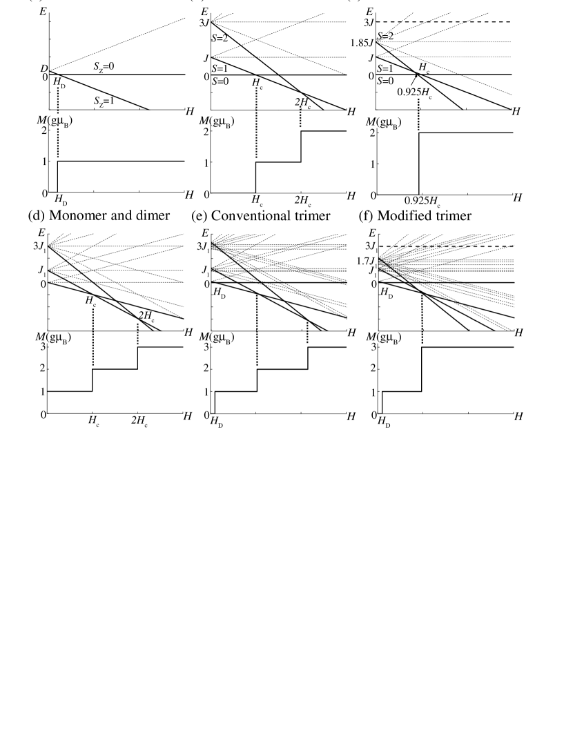
Figure 6: The field dependence of the energy levels and corresponding magnetization curve in $S$ = 1 spin cluster systems. (a) Monomer spin with a single-ion anisotropy D. (b) Conventional Heisenberg spin dimer. (c) Heisenberg spin dimer with the reduced energy levels of $S$ = 2 states. (d) Isolated monomer and dimer. (e) Conventional trimer where a dimer is weakly coupled to a monomer. Single-ion anisotropy is also considered. (f) The trimer with the reduced energy levels of higher energy states.

The magnetic field dependence of the energy level of Heisenberg $S$=1 spin dimer is shown in the upper panel of Fig. 6 (b), and the corresponding magnetization curve is shown in the lower panel. The magnetization curve exhibits $1/2$ plateau at $H_{c}\leq H\leq 2H_{c}$ with $H_{c}$ = $J/(g{\mu}_{B}),$ where the ground state is $\lvert S,S^{z}\rangle=\lvert 1,1\rangle$. In contrast in 0.22O₂-(Cu-CHD) the plateau is absentMori as shown in Fig. 7(a), and it seems more likely two-level system. Anomalous energy level of $S=1$ spin dimers in the adsorbed oxygen system was initially discussed in the temperature dependence of the neutron intensity in a different metal complex, CPL-1.Masuda The intensity decreased more rapidly with the increase of the temperature compared with conventional $S$ = 1 spin dimer model, suggesting the lowering of the energy level of the $S$ = 2 quintet state and the proximity to the triplet state of $S$ = 1. The energy level was explained based on the calculation including inter-molecular potential of O₂.Bussery For the dimer of O₂ molecules, both the ground state with $S$=0 and the first excited states with $S$=1 have an H-configuration shown in Fig. 5(e) in the equilibrium molecular positions. On the other hand, the second excited state with $S$ = 2 has an X-configuration shown in Fig. 5(f) of which the energy is lower than that in the H-configuration. The energy difference between $S$ = 0 and $S$ = 1 in both H configuration and that between $S$ = 1 in H configuration and $S$ = 2 in X configuration is almost the same, resulting in the anomalous energy level.

In the magnetization and x-ray study in 0.22O₂-(Cu-CHD), the lowering of the $S$ = 2 state was explained in the similar manner.Hori According to their Rietveld/MEM analysis $S$-geometry as shown in Fig. 5(g) was realized for $S$ = 2 state. It was estimated that the first energy-gap between $S=0$ and $S=1$ is 3.7 meV and the second one between $S=1$ and $S=2$ was 4.7 meV. The distribution of the exchange constant and the single-ion anisotropy term were not considered there. In the present paper we consider the magnetization data of both O₂/(Cu atom)=0.22 and 1.11 reported by W. Mori $et$ $al.$ Mori Our discussion is based on the spin monomer/dimer/trimer model with the normally distributed exchange constant and the single-ion anisotropy obtained from the INS spectra. We also assume that the eigenenergies of higher states calculated by conventional spin Hamiltonian are reduced because of the spin-dependent molecular potential in the oxygen dimer.Hemert ; Wormer ; Bussery ; Bussery94

We consider the following Hamiltonians

$$\mathcal{H}_{\rm mono} = D\sum_{l}\left(S_{l}^{z}\right)^{2}-g\mu_{B}H\sum_{l}S_{l}^{z^{\prime}}$$ (3)

$$\mathcal{H}_{\rm dimer} = J\mbox{\boldmath$S_{1}$}\cdot\mbox{\boldmath$S_{2}$}+D\sum_{l}\left(S_{l}^{z}\right)^{2}-g\mu_{B}H\sum_{l}S_{l}^{z^{\prime}}$$ (4)

$$\mathcal{H}_{\rm trimer} = J_{1}\mbox{\boldmath$S_{1}$}\cdot\mbox{\boldmath$S_{2}$}+J_{2}\mbox{\boldmath$S_{2}$}\cdot\mbox{\boldmath$S_{3}$}+D\sum_{l}\left(S_{l}^{z}\right)^{2}$$ (5)

$$- g\mu_{B}H\sum_{l}S_{l}^{z^{\prime}}$$

where the direction of the magnetic field, $H$, is defined as $z^{\prime}$-axis. For all models, we fixed $D$=0.41 meV. The magnetizations were calculated using the above Hamiltonians having the distributions in $J$ and $J_{1}$. The powder average was performed.

The reported magnetization in 0.22O₂-(Cu-CHD) exhibited a small increase below 5 T and a large increase at around 20 T with increasing $H$. The former increase is not explained by $S$ = 1 dimer model but by $S$ = 1 monomer model. As schematized in Fig. 6(a) the magnetization of the monomer at $T$ = 0 K exhibits a step function of which the jump field is $H_{D}=D/(g{\mu}_{B})$. Use the value of $D$ = 0.41 meV and $H_{D}$ = 3.5 T is obtained. At finite temperature the jump is smeared. The field scale of the initial increase of the magnetization is, thus, consistent with that of the single-ion anisotropy $D$ = 0.41 meV. We, therefore, assume that $S$ = 1 oxygen molecule monomers were trapped in some local minima in the nanopore or surface of the grain of the crystal in 0.22O₂-(Cu-CHD). The ratio of O₂ molecules in the monomer, $N$, is estimated to be 10 % of the total O₂ molecules from the magnetization plateau at $8{\rm T}\lesssim H\lesssim 15{\rm T}.$ The small number of the monomers would be the reason why the excitation was not observed in INS spectrum.

The red lines in Fig. 5(c) shows the energy levels of the spin dimer of which the energy of the quintet $S$ = 2 state is lowered compared with the conventional spin dimer. The field dependences of the conventional and modified states are shown in the upper panel in Fig. 6(b) and (c). The single-ion anisotropy is omitted for the simplicity here. In the modified scheme the energy of the $S^{z}$ = 2 crosses at the lower field than that of $S^{z}$ = 1 does, meaning that the magnetization curve is a single-step function as shown in the lower panel. By introducing the distribution of the exchange constant, the critical field is smeared and the experimentally obtained magnetization-curve is reproduced. We assume that the inflection point of the experimental magnetization curve is the critical field of the spin dimer having the mean value of $J$, 4.15 meV, in Table I. The field of the inflection is estimated to be 34 T, leading to that the decrease of the energy of the $S$ = 2 state, ${\Delta}E$, is 1.1$J$. Considering the single-ion anisotropy we found that 1.15$J$ is more appropriate value. The distribution of the $J$ is manually changed to find the best consistency. It is find that 1.77 meV is the best standard deviation of $J$. The magnetization curve calculated by using the parameters in Table I is indicated by the red solid curve in Fig. 7(a). The data is reasonably reproduced by the calculation. The blue solid curve is the magnetization for $\sigma$ = 0, meaning that the distribution of $J$ is required. The component of dimer and that of monomer is indicated by green solid curve and black dashed curve in Fig. 7(b).

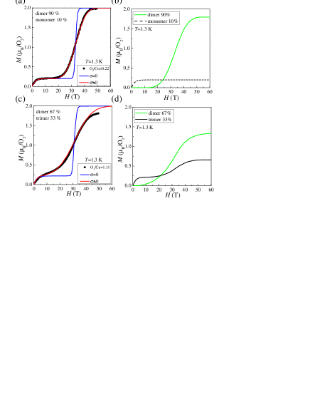
Figure 7: (Color online) Comparison between the magnetization reported by W. Mori $et$ $al.$Mori and the calculated magnetization. The black symbols show the reported data, and the blue and red solid lines represent the calculation (see text). (a) Magnetic field dependence of the magnetization for Cu-CHD adsorbing less oxygen molecules. (b) Temperature dependence of the magnetic susceptibility for Cu-CHD adsorbing less oxygen molecules. (c) Magnetic field dependence of the magnetization for Cu-CHD adsorbing more oxygen molecules. (d) Temperature dependence of the magnetic susceptibility for Cu-CHD adsorbing more oxygen molecules.

The lowering of the $S$ = 2 state is not probed in the INS profile because the transition between $S$ = 0 and $S$ = 2 is forbidden. The transition between $S$ = 1 and $S$ = 2 is not forbidden but is not observed because of the small probability of $S$ = 1 state at the low temperature. We note that the excitation at $E$$\simeq$2.4 meV observed in INS is not probed in the magnetization. The result supports our consideration that it is not from the magnetic origin.

The magnetization of 1.11O₂-(Cu-CHD) measured by Mori et al. Mori is indicated by solid symbols in Fig. 7(c). To understand the qualitative behavior of the $S$ = 1 trimer composed of a dimer weakly coupled to a monomer, it is instructive to consider an isolated monomer and dimer. The energy level and the corresponding magnetization curve is shown in Fig. 6(d). The magnetization exhibits three-step staircase where the critical fields are $H_{1,c}$ and $2H_{1,c}$ with $H_{1,c}=J_{1}/(g{\mu}_{B})$. The ground state is $S$ = 1 triplet and the magnetization has 1 $g{\mu}_{B}$/trimer even at 0 T. By introducing the weak coupling between dimer and monomer $J_{2}$ and the single-ion anisotropy $D$, the degenerated states are lifted and the energy levels and the corresponding magnetization curve are modified as shown in Fig. 7(e). Here the highest states are $\lvert S,S_{z}\rangle=\lvert 3,\pm 3\rangle$ and the energy is about $3J_{1}$. In order to make the magnetization a two-step staircase, it is necessary to lower the energies of the group of the higher states at about $3J_{1}$ by ${\Delta}E$ as shown in the upper panel in Fig. 6(f). By introducing the distribution of $J_{1}$ the step function is smeared. We tried to reproduce the experimental data by the trimers model but we failed. Instead the data was reproduced by the sum of the distributed dimers and the distributed trimers as indicated by red solid curve in Fig. 7(c). The ratio of O₂ in dimers is 67% of the total adsorbed O₂. In Fig. 7(d) the magnetization of the dimers and trimers are indicated by green and black solid curves, respectively. The parameters used in the calculation are summarized in Table II.

The concentration of O₂ in the sample used in magnetization measurement is 1.11[mole/f.u.], and it is smaller than that in INS measurement 2.0[mole/f.u.]. The less amount of O₂ would be the reason for the substantial number of dimers in the magnetization data. The data, however, indicates that some amount of dimers may be included also in the sample of 2.0O₂-(Cu-CHD) used in the INS experiment. The existence of several potential minima in the nanopore may be a possible reason for the inclusion of both dimers and trimers.

VI Conclusion

We performed INS measurements on Cu-CHD adsorbing O₂ molecules with the low and high concentrations to identify the magnetism of the O₂-based magnet realized in the nanopores. The INS spectra of the two different samples are explained by different spin Hamiltonians, spin dimers and spin trimers, meaning that the spin system can be controlled by the concentration of O₂ molecule in the O₂-based magnet. It is found that the magnetic excitation is broad and, therefore, the system is composed of a group of clusters having normally distributed exchange constants. This indicates that the supercrystal of the oxygen molecules is not perfect. By using the parameters obtained in INS and by assuming the reduction of the higher energy states due to the non-negligible spin-dependence in the molecular potential, magnetization curves are explained in quantitative level.

References

- (1) C. Uyeda, K. Sugiyama, and M. Date, J. Phys. Soc. Jpn. 54, 1107 (1985).
- (2) Y. A. Freiman and H. J. Jodl, Physics Reports 401, 1 (2004).
- (3) S. Desgreniers, Y.K. Vohra, and A.L. Ruoff, J. Phys. Chem. 94, 1117 (1990).
- (4) K. Shimizu, K. Suhara, M. Ikumo, M. Eremets, and K. Ameya, Nature 393, 767 (2998).
- (5) I. Goncharenko, O. Makarova, and L. Ulivi, Phys. Rev. Lett. 93, 055502 (2004).
- (6) M.C. van Hemert, P.E.S. Wormer, and A. van der Avoird, Phys. Rev. Lett. 51, 1167 (1983).
- (7) P.E.S. Wormer and Ad van der Avoird, J. Chem. Phys. 81, 1929 (1984).
- (8) B. Bussery and P. E. S. Wormer, J. Chem. Phys. 99, 1230 (1993).
- (9) B. Bussery, S. Ya. Umanskii, M. Aubert-Frécon, and O. Bouty, J. Chem. Phys. 101, 416 (1994).
- (10) K. Nozawa, N. Shima, and K. Makoshi, J. Phys. Soc. Jpn. 71, 377 (2002).
- (11) M. Obata, M. Nakamura, I. Hamada, and T. Oda, J. Phys. Soc. Jpn. 82, 093701 (2013).
- (12) J. P. McTague and M. Nielsen, Phys. Rev. Lett. 37, 596 (1976).
- (13) Y. Murakami and H. Suematsu, Phys. Rev. B 54, 4146 (1996).
- (14) S. Kitagawa, R. Kitaura, and S. Noro, Angew. Chem., Int. Ed. 43, 2334 (2004).
- (15) S. Takamizawa, E. Nakata, and T. Saito, Angew. Chem., Int. Ed. 43, 1368 (2004).
- (16) S. Takamizawa, E. Nakata, T. Akatsuka, C. Kachi-Terajima, and R. Miyake, J. Am. Chem. Soc. 130, 17882 (2008).
- (17) M. Kondo, T. Okubo, A. Asami, S. Noro, T. Yoshitomi, S. Kitagawa, T. Ishii, H. Matsuzaka, and K. Seki, Angew. Chem., Int. Ed. 38, 140 (1999).
- (18) W. Mori, T. C. Kobayashi, J. Kurobe, K. Amaya, Y. Narumi, T. Kumada, K. Kindo, H. Aruga Katori, T. Goto, N. Miura, S. Takamizawa, H. Nakayama, and K. Yamaguchi, Mol. Cryst. Liq. Cryst. 306, 1 (1997).
- (19) T. Masuda, S. Takamizawa, K. Hirota, M. Ohba, and S. Kitagawa, J. Phys. Soc. Jpn. 77, 083703 (2008).
- (20) D. Wallacher, R. Ackermann, P. Huber, M. Enderle, and K. Knorr, Phys. Rev. B 64, 184203 (2001).
- (21) R. Ackermann and M. Enderle, Europhys. Lett. 64, 260 (2003).
- (22) M. Hagiwara, M. Ikeda, T. Kida, K. Matsuda, S. Tadera, H. Kyakuno, K. Yanagi, Y. Maniwa, and K. Okunishi, J. Phys. Soc. Jpn. 83, 113706 (2014).
- (23) A. Hori, T. C. Kobayashi, Y. Kubota, A. Matsuo, K. Kindo, J. Kim, K. Kato, M. Takata, H. Sakamoto, R. Matsuda, and S. Kitagawa, J. Phys Soc. Jpn. 82, 084703 (2013).
- (24) M. Inoue, T. Atake, H. Kawaji, T. Tojo, Solid State Comm. 134, 303 (2005).
- (25) K. Nakajima, S. Ohira-Kawamura, T. Kikuchi, M. Nakamura, R. Kajimoto, Y. Inamura, N. Takahashi, K. Aizawa, K. Suzuya, K. Shibata, T. Nakatani, K. Soyama, R. Maruyama, H. Tanaka, W. Kambara, T. Iwahashi, Y. Itoh, T. Osakabe, S. Wakimoto, K. Kakurai, F. Maekawa, M. Harada, K. Oikawa, R. E. Lechner, F. Mezei, and M. Arai, J. Phys. Soc. Jpn. 80, SB028 (2011).
- (26) Y. Inamura, T. Nakatani, J. Suzuki, and T. Otomo, J. Phys. Soc. Jpn. 82, SA031 (2013).
- (27) S. Kimura, K. Kindo, Y. Narumi, M. Hagiwara, H. Kikuchi, and Y. Ajiro, J. Phys. Soc. Jpan. 72, 99 (2003).
- (28) M. Tinkham and M. W. Strandberg, Phys. Rev. 97, 937 (1955).
- (29) G.L. Squires, Introduction to the Theory of Thermal Neutron Scattering, (Cambridge University Press, Cambridge, 1978).
- (30) P. W. Stephens, Phys. Rev. B 31, 4491 (1985).