Imaging and Spectral Observations of Quasi-Periodic Pulsations in a Solar Flare

Abstract

We explore the Quasi-Periodic Pulsations (QPPs) in a solar flare observed by Fermi Gamma-ray Burst Monitor (GBM), Solar Dynamics Observatory (SDO), Solar Terrestrial Relations Observatory (STEREO), and Interface Region Imaging Spectrograph (IRIS) on 2014 September 10. QPPs are identified as the regular and periodic peaks on the rapidly-varying components, which are the light curves after removing the slowly-varying components. The QPPs display only three peaks at the beginning on the hard X-ray (HXR) emissions, but ten peaks on the chromospheric and coronal line emissions, and more than seven peaks (each peak is corresponding to a type III burst on the dynamic spectra) at the radio emissions. An uniform quasi-period about 4 minutes are detected among them. AIA imaging observations exhibit that the 4-min QPPs originate from the flare ribbon, and tend to appear on the ribbon front. IRIS spectral observations show that each peak of the QPPs tends to a broad line width and a red Doppler velocity at C I , O IV , Si IV , and Fe XXI lines. Our findings indicate that the QPPs are produced by the non-thermal electrons which are accelerated by the induced quasi-periodic magnetic reconnections in this flare.

1 Introduction

Quasi-Periodic Pulsations (QPPs) are regular phenomenons and common features observed in the solar flare emissions. In a typical event, QPP displays as the periodic peaks on the light curve. Each peak has a similar lifetime, which results in a regular interval among them. Therefore, the QPPs are characterized by the repetition or the periodicity. They are observed with the typical periods ranging from milliseconds (e.g., Karlický et al., 2005; Tan et al., 2010) through seconds (e.g., Hoyng et al., 1976; Lipa, 1978; Bogovalov et al., 1983, 1984; Mangeney & Pick, 1989; Zhao et al., 1991; Aschwanden et al., 1994b; Ning et al., 2005; Zimovets & Struminsky, 2010; Nakariakov et al., 2010) to minutes (e.g., Nakariakov et al., 1999; Aschwanden et al., 2002; De Moortel et al., 2002; Foullon et al., 2005; Ofman & Sui, 2006; Li & Gan, 2008; Sych et al., 2009; Tan et al., 2010; Su et al., 2012a; Ning, 2014). The previous observations show that their periods are positively correlated with the major radius of the flaring loop (Aschwanden et al., 1998). The short QPPs are thought to be associated with kinetic processes caused by the dynamic interaction of electromagnetic, plasma or waves with energetic particles trapped in closed magnetic fields (Aschwanden, 1987; Nakariakov & Melnikov, 2009). The long QPPs are usually associated with active region dynamics and global oscillations of the Sun (Chen & Priest, 2006; Nakariakov & Melnikov, 2009).

The QPPs are detected in a broad wavelength range from radio (e.g., Mangeney & Pick, 1989; Zhao et al., 1991; Aschwanden et al., 1994b; Kliem et al., 2000; Karlický et al., 2005; Ning et al., 2005; Tan et al., 2010) through visible and extreme-ultraviolet (EUV) (e.g., Nakariakov et al., 1999; Aschwanden et al., 2002; De Moortel et al., 2002; Ofman & Wang, 2002; Su et al., 2012a, b) to X-rays (e.g., Hoyng et al., 1976; Lipa, 1978; Bogovalov et al., 1983, 1984; Foullon et al., 2005; Ofman & Sui, 2006; Nakariakov et al., 2006; Li & Gan, 2008; Zimovets & Struminsky, 2010; Nakariakov et al., 2010; Ning, 2014), and even to $\gamma$-rays (Nakariakov et al., 2010). In radio emissions, the QPPs are usually detected as the periodic type III bursts. Mangeney & Pick (1989) have reported the periods range from 1 to 6 s. The statistical studies of the quasi-periodicity in the normal and reverse slope type III bursts have been reported by Aschwanden et al. (1994b) and Ning et al. (2005), respectively. Both of them obtained the mean period of $\sim$2 s and believed that the periodicity is due to the periodic acceleration processes in the solar flares. At EUV wavelengths, QPPs are usually detected in coronal loops. Moreover, using the spectral observations, the QPPs in Doppler velocity and line width of the hot and cool lines are also detected (Kliem et al., 2002; Tian et al., 2011). For example, using Solar Ultraviolet Measurement of Emitted Radiation (SUMER) spectrometer on board Solar and Heliospheric Observatory (SOHO), the Doppler velocity in hot lines ($>$ 6 MK) are detected to exhibit QPPs with period of about ten minutes (Ofman & Wang, 2002; Wang et al., 2002, 2003). With the Bragg Crystal Spectrometer (BCS) on Yohkoh, the Doppler velocity in the flare emission lines (e.g., S XV and Ca XIX ) is observed to display the QPPs with the period of serval minutes (Mariska, 2005, 2006). Tian et al. (2011) found that the QPPs are correlated with line intensity, Doppler velocity, and line width from the observations of Hinode EUV Imaging Spectrometer (EIS). In the X-ray and $\gamma$-ray channels, the QPPs with a short period of a few seconds are detected by Hoyng et al. (1976) and Bogovalov et al. (1983). Using Reuven Ramaty High-Energy Solar Spectroscopic Imager (RHESSI) observations, the 2005 January 19 solar flare displays the QPPs with a period of 2$-$4 minutes at HXR emissions (Ofman & Sui, 2006), while the 2002 December 26 solar flare exhibits the 2-min QPPs at the soft X-ray (SXR) emissions (Ning, 2014). Some flares exhibit similar QPPs in a broad wavelengths (e.g., Nakajima et al., 1983; Aschwanden et al., 1995; Asai et al., 2001). For example, the 1998 November 10 solar flare displays the QPPs with a period of 6 s in both radio and X-ray emissions (Asai et al., 2001), while Nakajima et al. (1983) reported the QPPs with a quasi-period of 8 s from radio, hard X-ray (HXR) and $\gamma$-ray emissions.

The generation mechanism of QPPs is still an open issue in the documents (Aschwanden, 1987; Nakariakov et al., 2006; Li & Gan, 2008; Nakariakov & Melnikov, 2009; Ning, 2014). Basically, QPPs are thought to be related with the waves or energetic particles (electrons). Actually, MHD waves, such as slow magnetoacoustic waves, fast kink and sausage waves (Roberts et al., 1984; Nakariakov & Melnikov, 2009) have been used to explain the generation of the QPPs in radio (Nakariakov et al., 2004; Tan et al., 2010; Kupriyanova et al., 2010), EUV (Ofman & Wang, 2002; Mariska, 2006; Tian et al., 2011; Su et al., 2012a, b) and X-ray or $\gamma$- ray (Nakariakov et al., 2004; Foullon et al., 2005; Zimovets & Struminsky, 2010; Nakariakov et al., 2010) emissions. On the other hand, the QPPs could be explained by the emissions from the non-thermal electrons that are accelerated by the quasi-periodic magnetic reconnection. And the quasi-periodic reconnection can be spontaneous (Kliem et al., 2000; Karlický, 2004; Karlický et al., 2005; Murray et al., 2009) or may be modulated by MHD waves, i.e., the slow waves (Chen & Priest, 2006; Nakariakov & Zimovets, 2011; Li & Zhang, 2015) or the fast waves (Nakariakov et al., 2006; Nakariakov & Melnikov, 2009; Ofman & Sui, 2006; Liu et al., 2011). Until now, QPPs are poorly observed in a same flare with the imaging and spectral observations simultaneously, which could provide an opportunity to improve the QPPs origination and physics model. In this paper, we analyze the QPPs in a solar flare on 2014 September 10 observed by Fermi, SDO, STEREO, and IRIS at HXR, EUV, and radio wavelengths.

2 Observations and Data Analysis

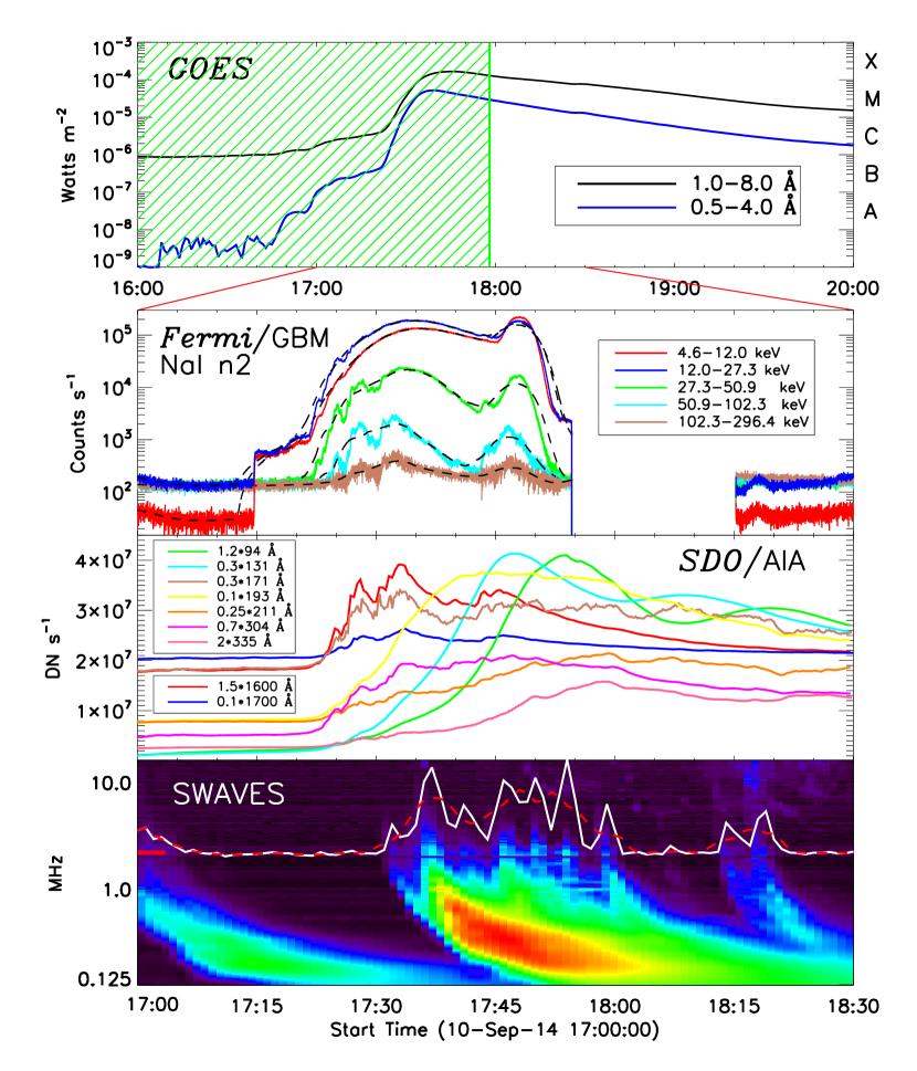
Figure 1: Top: GOES SXR flux from 16:00 UT to 20:00 UT on 2014 September 10. The vertical green line marks the end time of IRIS observations. Second: X-ray light curves from Fermi/GBM (detector n2) at 5 energy channels. The dashed lines represent the slowly-varying components. Third: AIA light curves integrated from the flare region marked with the blue box in Fig. 3. Bottom: radio dynamic spectra between 0.125$-$16.075 MHz from STEREO/WAVES. The white profile is the radio emission at frequency of $\sim$2.19 MHz which marked with the short red line, and the red dashed line represents the slowly-varying components.

The solar flare studied in this paper takes place in NOAA AR12158 (N11^∘, E05^∘) on 2014 September 10, and it is accompanied with a halo coronal mass ejection (CME). It is an X1.6 flare, which starts at 17:21 UT and reaches its maximin at 17:45 UT from GOES SXR flux. Fig. 1 shows the light curves detected by GOES, Fermi/GBM, and SDO/AIA, the dynamic spectra detected by STEREO/WAVES (SWAVES). The top panel gives the GOES observations at two SXR channels, such as 1.0$-$8.0 Å (black) and 0.5$-$4.0 Å (blue). The shaded interval marks IRIS observations. The second panel shows the Fermi light curves at 5 energy channels, such as 4.6$-$12.0 keV, 12.0$-$27.3 keV, 27.3$-$50.9 keV, 50.9$-$102.3 keV, and 102.3$-$296.4 keV. They are detected by the n2 detector, whose direction angle to the Sun is stable ($\sim$60^∘) during this flare, especially at the interval from 17:10 UT to 17:45 UT, while the other detectors change their direction angles frequently. After 17:45 UT, the n2 detector shifts its direction angle from $\sim$60^∘ to $\sim$45^∘, then become bigger again, which results into a X-ray peak around 17:50 UT. Therefore, it is not the real X-ray emission peak. There is a data gap after 17:54 UT. The time resolution of Fermi is 0.256 s, but becomes to 0.064 s automatically in the flare state (Meegan et al., 2009). We interpolate all the data into an uniform resolution of 0.256 s in the second panel. Such a cadence is enough to analyze the QPPs with a period of several minutes in this paper. The third panel shows the SDO/AIA light curves (integration from images) at 9 wavelengths, such as 1600 Å, 1700 Å, 94 Å, 131 Å, 171 Å, 193 Å, 211 Å, 304 Å, 335 Å. Their time resolutions are 24 s here. The bottom panel displays the radio dynamic spectra between $\sim$0.125 MHz and $\sim$16.075 MHz observed by SWAVES aboard STEREO_B. The time resolution is 1 minute (Rucker et al., 2005). There is a group of solar radio type III bursts.

Fig. 1 shows that there are several peaks during the impulsive phase at HXR light curves, i.e., from 17:21 to 17:40 UT. These peaks seem to be regular and periodic, and they looked like the QPPs. However, they are superposed by a gradual background emission. Meanwhile, there are several type III bursts on the dynamic spectra. The radio light curve at 2.19 MHz (white line) exhibits the regular peaks with a quasi-period. In order to distinguish these peaks from the background, we decompose each light curve at X-ray and radio bands into a slowly-varying component and a rapidly-varying component. The slowly-varying component (the background emission) is the smoothing original data. Here the smoothing window is different for various data with the similar cadences. For example, the smoothing window is 1000 points for Fermi data and 4 points for SWAVES data. The dashed lines over-plotted on the original light curves in Fig. 1 are their slowly-varying components.

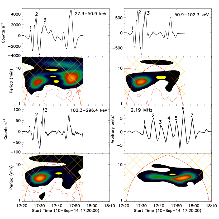
Figure 2: Top: the rapidly-varying components at Fermi 27.3$-$50.9 keV, 50.9$-$102.3 keV, 102.3$-$296.4 keV, and radio emission at frequency of $\sim$2.19 MHz. Bottom: their wavelet power spectra.

QPPs are identified from the rapidly-varying components, which are the light curves subtracted by the slowly-varying components. As shown in Fig. 1, we get the slowly-varying components at five X-ray bands (black dashed lines) and at one radio frequency (red dashed lines). Fig. 2 gives the rapidly-varying components at three HXR channels of 27.3$-$50.9 keV, 50.9$-$102.3 keV, and 102.3$-$296.4 keV and one radio frequency at $\sim$2.19 MHz. These three HXR channels display the typical QPPs with three regular peaks which marked by the number of ‘1’, ‘2’, and ‘3’ between 17:24 UT and 17:36 UT. There are no similar peaks in the other two X-ray bands below 27 keV. However, there are seven regular peaks between 17:32 and 18:01 on the radio frequency at $\sim$2.19 MHz, marked by the numbers. Then the wavelet analysis is used to detect the period of the QPPs. The bottom panels of Fig. 2 show their wavelet power spectra, which confirm the QPPs feature with a similar period of about 4 minutes at both HXR and radio emissions. As mentioned earlier, the HXR peaks at 17:50 UT are not real, although they are the emissions from the Sun.

There are two interesting facts to be mentioned here. Firstly, the HXR light curves display the QPPs from 17:24 UT to 17:36 UT, while the radio emissions exhibit the QPPs from 17:32 UT to 18:01 UT. Namely, there is a delay of about 8 minutes between their onset. Secondly, the QPPs show three peaks at HXR channels, but more than seven peaks at radio frequency. Each peak is a type III burst on the dynamic spectra. The question is whether the QPPs at HXR are related to that at the radio in this event, and whether the QPPs at HXR and radio originate the same process during the flare? In order to answer these questions, imaging and spectral analyses of the QPPs are needed. High spatial and time resolutions images of SDO/AIA and high spectral resolution of IRIS observations give us the opportunity to study the QPPs origination in the 2014 September 10 flare.

Fig. 3 shows the SDO/AIA 1600 Å, 131 Å and 304 Å images and the IRIS/SJ 1400 Å images at 17:30 UT before the flare maximum. Same as the other X-class flares, this event displays double ribbons at 1600 Å. One is short near the sunspot, while the other one is long and shows a curved shape. The light curves integrated in the blue box are given in the third panel of Fig. 1 at all 9 AIA wavelengths. AIA has a pixel size of 0$\farcs$6 and a time resolution of 24 s at 1600 Å and 1700 Å, while 12 s at the other 7 EUV wavelengths (Lemen et al., 2012). For the 2014 September 10 flare, AIA images at these seven EUV wavelengths are regularly saturated every 24 s. These saturation images are ruled out to do the analysis. The light curves at these 7 EUV wavelengths also have the time resolution of 24 s as same as that at 1600 Å and 1700 Å. The slit-jaw images (SJI) aboard IRIS take the solar images with a FOV (field of view) of 119$\arcsec$ $\times$ 119$\arcsec$ and pixel size of 0$\farcs$166. The time cadence is 19 s at 1400 Å and 2796 Å. The right upper panel in Fig. 3 gives one SJI at 1400 Å and it also includes the long ribbon of the solar flare. The AIA and SJ images have been pre-processed with the standard solar-software routines (Marc & Greg, 2013; Mclntosh et al., 2013) to be aligned. The AIA images at 1600 Å are used to co-align with the SJ images at 1400 Å because both of them include the continuum emissions from the temperature minimum, and the continuum emissions are dominant in many of the bright features. The upper middle and right panels in Fig. 3 show the results of the co-alignment between AIA 1600 Å and SJ 1400 Å images at 17:30 UT. They have the same scales, and similar bright features. The black line indicates the IRIS slit position. The red box in the left panels marks the FOV of the SJ image in the active region. Fig. 3 also shows the same regions at AIA 131 Å and AIA 304 Å, which correspond to the high and low temperatures, respectively. We make the movie for Fig. 3 from 17:12 UT to 17:58 UT, which contains the impulsive phase of the X1.6 flare (seen, f3.mpg).

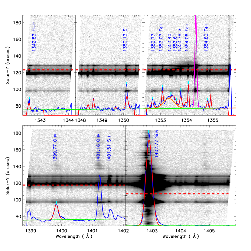
Figure 4: IRIS spectra at 17:30 UT from FUV1 (upper) (e.g., 1343, Fe XII 1349 and O I 1356) and FUV2 (bottom) bands (e.g., Si IV 1403). The blue spectral profiles are from the flare ribbon at the slit positions marked by the red dashed lines. The horizontal green lines mark the background profiles. The orange profile is the Fe XXI fitting, and the purple profile is the C I fitting. The main lines used to fit for this flare are labeled and indicated by the turquoise vertical ticks just above the line spectra.

IRIS spectrograph observes the AR12158 from 11:28 UT to 17:58 UT on 2014 September 10 in a “sit-and-stare” mode, and the step cadence is $\sim$9.4 s. The pixel size along the slit is $\sim$0$\farcs$166, and the spectral scale is $\sim$12.8 mÅ/pixel at FUV (FUV1 and FUV2) bands (Mclntosh et al., 2013; De Pontieu et al., 2013, 2014). But to save telemetry, two times spectral binning and a restricted number of spectral windows were obtained, i.e., the spectral scale is 25.6 mÅ/pixel, equivalent to 5.6 km s^-1/pixel. In this case, we used the ‘flare’ list of lines which are consisted of the ‘1343, Fe XII , O I , Si IV ’ windows. Fig. 4 shows the IRIS spectra of FUV1 (e.g., 1343, Fe XII 1349 and O I 1356) and FUV2 (e.g., Si IV 1403) windows at 17:30 UT. They have been processed to remove the bad pixels. Four lines at Fe XXI 1354.09 Å, C I 1354.33 Å, O IV 1399.77 Å, and Si IV 1402.77 Å are selected to do analysis. The former two lines are in the FUV1 window, while the O IV and Si IV lines are in the FUV2. It is well known that the forbidden line of Fe XXI 1354.09 Å is a broad line and it is always blended with other narrow lines from chromospheric emissions, especially the chromospheric line of C I 1354.33 Å (e.g., Doschek et al., 1975; Cheng et al., 1979; Mason et al., 1986; Innes et al., 2003a, b), which makes it difficult to fit. IRIS has a high spectral resolution of $\sim$26 mÅ, which results into distinguishing a lot of bright emission lines. The upper panel of Fig. 4 shows that some of them are well identified, such as C I 1354.33 Å (purple line), Fe II 1353.07 Å and 1354.06 Å, Si II 1353.78 Å, but some of them are still not identified, i.e., 1352.77 Å, 1353.40 Å, and 1353.61 Å. These known and unknown bright emission lines which blend with the Fe XXI line must be extracted before determining the Fe XXI intensity. In this case, the fit method described by Li et al. (2015) are used to extract the Fe XXI line information. Briefly, we fix these bright emission line positions, constrained their widths and tied their intensities to the lines in other spectral windows. Finally, 15 Gaussian lines superimposed on a linear background are fitted across the whole wavelength region. Only 11 lines are marked with the turquoise vertical ticks in the upper panel of Fig. 4. Thus we can detect the integral intensities, line widths and Doppler velocities of these lines simultaneously in each fitting, including the chromospheric line of C I 1354.33 Å and the coronal line of Fe XXI 1354.09 Å. The bottom panel of Fig. 4 shows the FUV2 windows with four lines, such as O IV 1399.77 Å and 1401.16 Å, S I 1401.51 Å and Si IV 1402.77 Å. Two lines ( O IV 1401.16 Å and S I 1401.51) are ruled out to analyze because they are blended with each other, especially during the flare time. The other two lines are isolated and can be well fitted with a single Gaussian function (red lines) to detect the integral intensities, line widths and Doppler velocities.

3 Results

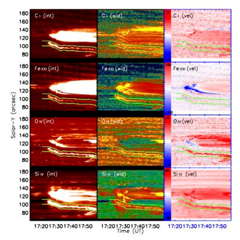
Figure 5: The space-time diagrams of line intensity (left), line width (middle) and Doppler velocity (right) from IRIS observations, such as C I , Fe XXI , O IV , and Si IV lines. The light curves integrated between two green lines are shown in Fig. 6.

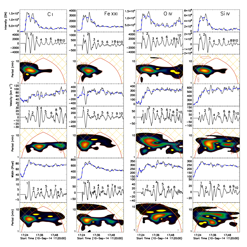
Figure 6: Time evolution of intensity (row 1), Doppler velocity (row 4), and line width (row 7) at the lines of C I (column 1), Fe XXI (column 2), O IV (column 3), and Si IV (column 4). The blue dashed lines represent the slowly-varying components. Rows (2, 5, 8): their rapidly-varying components. Rows (3, 6, 9): their wavelet power spectra.

Fig. 5 shows the space-time diagrams of the line intensity, line width and Doppler velocity after fitting four lines at C I 1354.33 Å, Fe XXI 1354.09 Å, O IV 1399.77 Å and Si IV 1402.77 Å) from 17:12 to 17:58 UT. The Y-axis is along the slit, which is fixed on the solar disk. This fact results into the IRIS slit observes the same region of the flare ribbon during this interval, as seen in the movie (f3.mpeg). There are two strong emission patterns on these space-time diagrams. The northern one is wide, and the southern pattern is narrow. This is because the slit straddles on the curved flare ribbon, as shown in Fig. 3. These two emission patterns are just the different parts of this ribbon. Different from the wide (northern) pattern, the narrow one display the intensity variation with the time, including the C I , Fe XXI , O IV , and Si IV lines. This behavior is similar as the QPPs shown in the HXR and radio emissions. In order to analyze this feature in detail, we firstly use two lines to trace the southern narrow emission pattern, as shown in Fig. 5. The distance between these two lines is a constant of about 10$\arcsec$, as the distance along the slit between two short green lines in Fig. 3. Secondly, the intensities between these two lines are integrated. Thus, we get the intensity light curves of C I , Fe XXI , O IV , and Si IV lines. Fig.6 shows that there are ten peaks on their intensity light curves from 17:24 UT to 17:56 UT, roughly with a quasi-period of less than 4 minutes. It is clear that these peaks are superposed on a gradual component. Using the same method as shown in Fig. 2, Fig. 6 (upper-left panel) shows that the C I light curve is decomposed into a slowly-varying and a rapidly-varying components. The slowly-varying component is smoothing a window of 28 points. The rapidly-varying component is the C I light curve subtracting the slowly-varying component. These ten peaks are clearly shown as marked by the numbers, and they are identified as the QPPs. The wavelet spectra confirm the quasi-period of less than 4 minutes. Such QPPs are also distinctly detected from the O IV and Si IV light curves. There are some signatures of the QPPs on Fe XXI light curves, especially the first three peaks. The other seven peaks of Fe XXI line are weak. Fig. 6 gives the temporal evolution of the Doppler velocities and line widths at C I , Fe XXI , O IV , and Si IV lines. The flare ribbon displays the red shifts on the Doppler velocities of these four lines. And the mean velocities between 17:24 UT and 17:58 UT are 67.4 km s^-1, 121.4 km s^-1, 297.9 km s^-1, and 535.7 km s^-1 at C I , Fe XXI , O IV , and Si IV lines, as listed in table 1. There are also some peaks on the Doppler velocities corresponding to that on the intensities, but not one-by-one. The flare ribbon exhibits a broad line widths  and the mean values between 17:24 UT and 17:58 UT are 73.9 pixels, 514.1 pixels, 291.2 pixels, and 247.3 pixels at C I , Fe XXI , O IV , and Si IV lines (see, table 1). There are some peaks on the line widths corresponding to the QPPs peaks too. Using the same method, their Doppler velocities and line widths are decomposed into the slowly-varying and rapidly-varying components. The wavelet spectra of the rapidly-varying components of Doppler velocity and line width also exhibit the similar 4-min QPPs features.

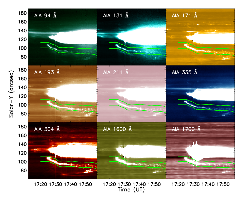
Figure 7: Same as Fig. 5, but the space-time diagrams at 9 AIA wavelengths from the same position as the IRIS slit.

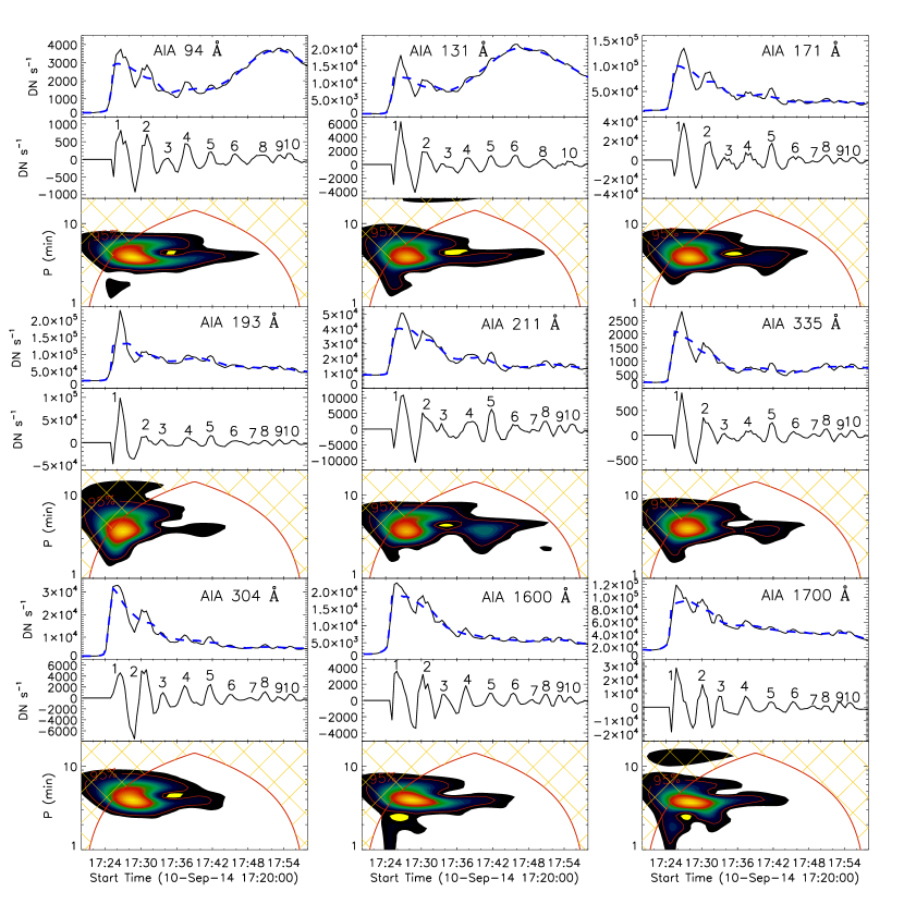
Figure 8: Rows (1, 4, 7): the light curves integrate between two green lines in Fig. 7 at all AIA 9 wavelengths. The blue dashed lines are the slowly-varying components. Rows (2, 5, 8): their rapidly-varying components. Rows (3, 6, 9): their wavelet power spectra.

SDO/AIA movie shows that the flare ribbon evolve from the northeast toward the southwest on the solar disk, which results into the flare ribbon cross the IRIS slits. The onset time at 17:24 UT in Fig. 6 is not the flare beginning time but represents the starting time of the flare ribbon entrance into the slit window. It is hard to detect the QPPs starting time from the flare ribbon. However, an artificial slit with a position same as IRIS slit is put on the AIA images. Thus we get the space-time diagrams from AIA observations, as shown in Fig. 7. Same as the IRIS observation in Fig. 5, there are two bright patterns corresponding to the two parts of the flare ribbon. There are intensity flashes at the southern small region. Using the same two lines in Fig. 5, the light curves between them are shown in Fig. 8 at 9 AIA wavelengths. The QPPs are clearly seen on their light curves. Ten individual peaks are recognized between 17:24 UT and 17:56 UT, which is same as the IRIS observations, and each peak of QPPs is marked with numbers. The light curves are also decomposed into the slowly-varying (blue dashed line) and rapidly-varying components, whose wavelet spectra are also shown. The QPPs exhibit a period of less than 4 minutes again, which is similar to that in the spectral lines at C I , Fe XXI , O IV , and Si IV from IRIS observations.

4 Conclusions and Discussions

Based on the multi-wavelengths observations from Fermi/GBM, SDO/AIA, IRIS and SWAVES, we analyze the imaging and spectral observations of the 4-min QPPs at HXR, EUV, and radio emissions in a solar flare on 2014 September 10. We draw the conclusions as following:

(I) The 4-min QPPs are found in a broad frequency range from HXR through EUV to the radio.

(II) Imaging observations of SDO/AIA show that the QPPs originate from the flare ribbon front.

(III) Spectral observations of IRIS present that the QPPs peaks tend to a broad line width and a red-shift velocity.

Although there are several models to explain the QPPs in the documents (e.g., Aschwanden, 1987; Nakariakov et al., 2004; Nakariakov & Melnikov, 2009), our findings support that the QPPs are produced by the non-thermal electron beams accelerated by the periodic magnetic reconnection in this flare. In this case, each individual peak of the QPPs are radiated by the different electron beams. Based on the standard flare model, each magnetic reconnection can accelerate the bi-directional electron beams simultaneously (e.g., Heyvaerts et al., 1977; Aschwanden et al., 1995; Innes et al., 1997; Ning et al., 2000; Ji et al., 2006, 2008; Shen et al., 2008; Feng et al., 2011; Feng & Wang, 2013; Su et al., 2013; Zhang et al., 2012, 2014). The upward beam radiates the type III bursts on its trajectory propagation outer the corona. The downward beam produces one peak at HXR when it injects into the chromosphere to heat the local plasma on its way producing one peak at EUV. In this case, the periodic magnetic reconnection can produce the QPP peaks at HXR and radio type III bursts, and the periodic EUV emissions as well. In other words, the periodic magnetic reconnection model can well explain the QPPs from HXR through EUV to the radio emissions in 2014 September 10 solar flare. In general, the other models also explain the QPPs features, especially at HXR and EUV bands (e.g., Ofman & Wang, 2002; Foullon et al., 2005; Su et al., 2012a), i.e., the MHD flux tube oscillations, modulated by certain waves or periodic self-organizing systems of plasma instabilities. As mentioned earlier, solar type III bursts are produced by the electron beams propagating into the outer corona, then into the interplanetary. In other words, a group of type III bursts are produced by various electron beams. Therefore, the periodic solar type III bursts provide direct evidence of the periodic magnetic reconnection in this flare.

It is still an open question what does determine the period? The quasi-periodic magnetic reconnection may be spontaneous (Kliem et al., 2000; Karlický, 2004; Karlický et al., 2005; Murray et al., 2009), or could be modulated by certain waves in solar corona (Aschwanden et al., 1994a; Aschwanden, 2004; Chen & Priest, 2006; Ofman & Sui, 2006; Nakariakov et al., 2006; Inglis & Nakariakov, 2009; Nakariakov & Zimovets, 2011; Liu et al., 2011; Li & Zhang, 2015). If in the case of spontaneous quasi-periodicity it is not understood yet what determines the period (e.g., Kliem et al., 2000; Murray et al., 2009). If in the latter induced case, the periodic triggering of the reconnection can be some MHD oscillations, as were shown in several papers (e.g., Chen & Priest, 2006; Nakariakov et al., 2006; Nakariakov & Zimovets, 2011). The period of the observational QPPs is thought to be associated with one of the MHD modes. There are three possibilities for such MHD wave modes which may trigger the periodic magnetic reconnection in our case. The first possibility is the quasi-periodic reconnection modulated by slow waves (Chen & Priest, 2006). For example, the 3 or 5-min solar p-mode oscillations (slow waves) can trigger the quasi-periodic magnetic reconnection with the similar period when the reconnection site is located in the upper chromosphere (Ning et al., 2004). This is similar to 4-min period of QPPs in the 2014 September 10 flare. However, this model depends strongly on the location of the reconnection site in the solar atmosphere, and it becomes weaker when the reconnection site is lower or higher than the upper chromosphere. The second possibility is the quasi-periodic reconnection modulated by fast waves. Nakariakov et al. (2006) suggest that the fast waves in a corona loop situated near the flare site can trigger the quasi-periodic magnetic reconnection. In particular, the global kink mode (Foullon et al., 2005) can trigger the quasi-periodic magnetic reconnection and produce the QPPs with a period of about several minutes. This model is used to explain the min-periodic phenomena in solar flares. The third case is the slow magnetoacoustic waves to modulate the quasi-periodic reconnection. Nakariakov & Zimovets (2011) have demonstrated that the slow magnetoacoustic waves can propagate along the axis of a coronal magnetic arcade, then possibly to trigger the quasi-periodic reconnection during the solar flare. The observational period is similar to the period of a standing slow magnetoacoustic wave in the loops that form the arcade. They suggest that the quasi-periodic pulsations observed in two-ribbon flares can be explained with this mechanism. Namely, such mechanism can explain the 4-min period of QPPs in 2014 September 10 flare. This is because we find that the brightness structures move along the flare ribbon parallel to the magnetic neutral line (seen the movie of f3.mpeg). Fig. 9 (upper panel) shows the space-time slices along the flare ribbon A$\rightarrow$B on AIA 1600 Å image in Fig. 3. There are many brightening structures moving from A to B. The propagation speed is roughly estimated about 15$-$40 km s^-1, which is consistent with previous findings (e.g., Bogachev et al., 2005; Krucker et al., 2005; Tripathi et al., 2006; Li & Zhang, 2009; Reznikova et al., 2010; Nakariakov & Zimovets, 2011; Li & Zhang, 2015). And these values are much smaller than the local Alfvén and sound speeds. The moving brightening structures are thought to be the evidences of the slow magnetoacoustic waves across the magnetic fields in solar flares (Nakariakov & Zimovets, 2011).

The delay of about 8 minutes between the HXR (or EUV) and radio emissions in this flare is possibly due to the different sites of the radio sources (electron beams for type III bursts) from HXR or EUV sources. Usually, HXR and EUV emissions are produced at the chromosphere or lower corona, while the radio source around 2 MHz originates from a heliocentric height of about 10R_⊙ (Krupar et al., 2014). The time of the electron beams (type III bursts source) propagating from the flare site (acceleration region) to $\sim$10R_⊙ roughly equals to the delay between HXR (or EUV) and radio emissions. Based on this assumption, we estimate that the electron beams (radio sources) have a speed of $\sim$0.05 $c$ ($c$ is the light speed in the vacuum). This value is reasonable for the electron beams propagate outward from the Sun in the interplanetary medium (e.g., Dulk et al., 1987; Krupar et al., 2014). Fig. 9 (bottom) plots the QPPs at IRIS C I intensity, AIA 171 Å, Fermi 27.3$-$50.3 keV, and SWAVES 2.19 MHz. Each peaks of the QPPs at C I intensity is well corresponding to that at AIA 171 Å. However, they are not correlated to the HXR and radio peaks, which could be resulted from the radiation source positions.

Table 1: The mean value and standard deviation on Doppler velocities and line widths between 17:24 UT and 17:58 UT of the spectral lines from IRIS observations.

Spectrum	Doppler velocity (km s-1)		Line width (pixels)
	Mean	Standard deviation	Mean	Standard deviation
C I	67.4	17.9	73.9	5.1
Fe XXI	121.4	140.4	514.1	91.2
O IV	297.9	55.7	291.2	27.8
Si IV	535.7	65.9	247.3	16.8

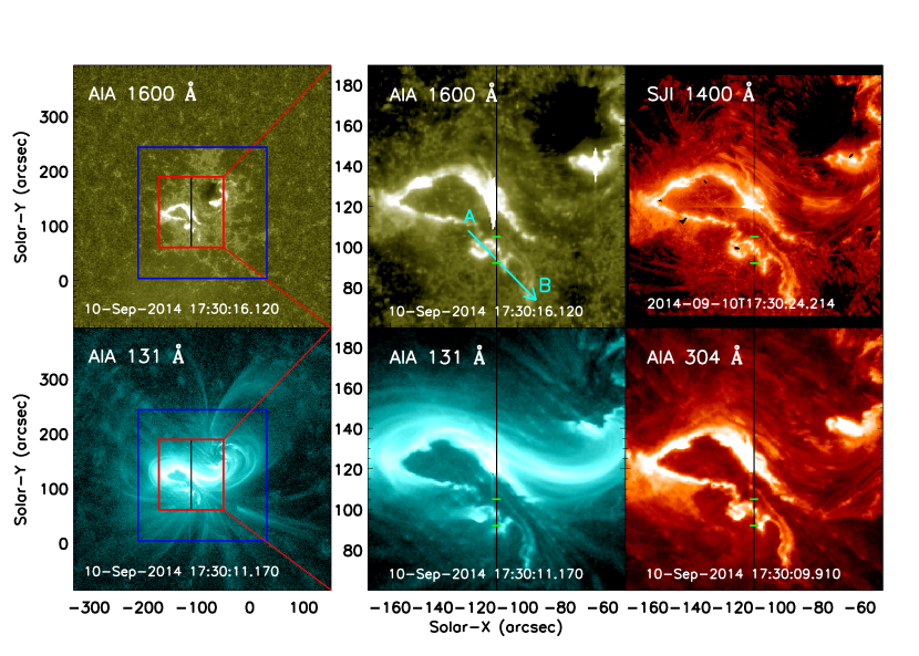
Figure 3: SDO/AIA and IRIS/SJ images at 17:30 UT on 2014 September 10. Left: AIA images at 1600 Å and 131 Å. The blue box marks the flare region to integrate the light curves in Fig. 1, and the red box give the FOV of the SJ image. The vertical black lines mark the IRIS slit positions. Right: AIA images at 1600 Å, 131 Å, and 304 Å with the same FOV of SJ image at 1400 Å. Two green solid lines mark a distance of about 10$\arcsec$ along the slit (see detail in the text). Arrow ‘A$\rightarrow$B’ marks the slit of the space-time diagram in Fig. 9.

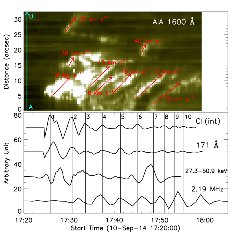
Figure 9: Upper: AIA 1600 Å space-time diagram along the slit ‘A$\rightarrow$B’ in Fig. 3. Bottom: the illustration of the QPPs at IRIS C I line, AIA 171 Å, Fermi 27.3$-$50.9 keV, and SWAVES 2.19 MHz.

References

- Asai et al. (2001) Asai, A., Shimojo, M., Isobe, H., et al. 2001, ApJ, 562, L103
- Aschwanden (1987) Aschwanden, M. J. 1987, Sol. Phys., 111, 113
- Aschwanden et al. (1994a) Aschwanden, M. J., Benz, A. O., Dennis, B. R., & Kundu, M. R. 1994a, ApJS, 90, 631
- Aschwanden et al. (1994b) Aschwanden, M. J., Benz, A. O., & Montello, M. L. 1994b, ApJ, 431, 432
- Aschwanden et al. (1995) Aschwanden, M. J., Benz, A. O., Dennis, B. R., & Schwartz, R. A. 1995, ApJ, 455, 347
- Aschwanden et al. (1998) Aschwanden, M. J., Kliem, B., Schwarz, U., et al. 1998, ApJ, 505, 941
- Aschwanden et al. (2002) Aschwanden, M. J., de Pontieu, B., Schrijver, C. J., & Title, A. M. 2002, Sol. Phys., 206, 99
- Aschwanden (2004) Aschwanden, M. J. 2004, ApJ, 608, 554
- Bogachev et al. (2005) Bogachev, S. A., Somov, B. V., Kosugi, T., & Sakao, T. 2005, ApJ, 630, 561
- Bogovalov et al. (1983) Bogovalov, S. V., Iyudin, A. F., Kotov, Y. D., et al. 1983, Soviet Astronomy Letters, 9, 163
- Bogovalov et al. (1984) Bogovalov, S. V., Iyudin, A. F., Kotov, Y. D., et al. 1984, Soviet Astronomy Letters, 10, 286
- Chen & Priest (2006) Chen, P. F., & Priest, E. R. 2006, Sol. Phys., 238, 313
- Cheng et al. (1979) Cheng, C.-C., Feldman, U., & Doschek, G. A. 1979, ApJ, 233, 736
- De Moortel et al. (2002) De Moortel, I., Ireland, J., Hood, A. W., & Walsh, R. W. 2002, A&A, 387, L13
- De Pontieu et al. (2013) De Pontieu, & Lemen, J. R. IRIS Technical Note 1 - IRIS operations, version 17: 22 Jul 2013
- De Pontieu et al. (2014) De Pontieu, B., Title, A. M., Lemen, J. R., et al. 2014, Sol. Phys., 289, 2733
- Doschek et al. (1975) Doschek, G. A., Dere, K. P., Sandlin, G. D., et al. 1975, ApJ, 196, L83
- Dulk et al. (1987) Dulk, G. A., Goldman, M. V., Steinberg, J. L., & Hoang, S. 1987, A&A, 173, 366
- Feng & Wang (2013) Feng, H., & Wang, J. 2013, A&A, 559, A92
- Feng et al. (2011) Feng, H. Q., Wu, D. J., Wang, J. M., & Chao, J. W. 2011, A&A, 527, A67
- Foullon et al. (2005) Foullon, C., Verwichte, E., Nakariakov, V. M., & Fletcher, L. 2005, A&A, 440, L59
- Heyvaerts et al. (1977) Heyvaerts, J., Priest, E. R., & Rust, D. M. 1977, ApJ, 216, 123
- Hoyng et al. (1976) Hoyng, P., van Beek, H. F., & Brown, J. C. 1976, Sol. Phys., 48, 197
- Inglis & Nakariakov (2009) Inglis, A. R., & Nakariakov, V. M. 2009, A&A, 493, 259
- Innes et al. (1997) Innes, D. E., Inhester, B., Axford, W. I., & Wilhelm, K. 1997, Nature, 386, 811
- Innes et al. (2003a) Innes, D. E., McKenzie, D. E., & Wang, T. 2003a, Sol. Phys., 217, 267
- Innes et al. (2003b) Innes, D. E., McKenzie, D. E., & Wang, T. 2003b, Sol. Phys., 217, 247
- Ji et al. (2006) Ji, H., Huang, G., Wang, H., et al. 2006, ApJ, 636, L173
- Ji et al. (2008) Ji, H., Wang, H., Liu, C., & Dennis, B. R. 2008, ApJ, 680, 734
- Karlický (2004) Karlický, M. 2004, A&A, 417, 325
- Karlický et al. (2005) Karlický, M., Bárta, M., Mészárosová, H., & Zlobec, P. 2005, A&A, 432, 705
- Kliem et al. (2002) Kliem, B., Dammasch, I. E., Curdt, W., & Wilhelm, K. 2002, ApJ, 568, L61
- Kliem et al. (2000) Kliem, B., Karlický, M., & Benz, A. O. 2000, A&A, 360, 715
- Krucker et al. (2005) Krucker, S., Fivian, M. D., & Lin, R. P. 2005, Advances in Space Research, 35, 1707
- Krupar et al. (2014) Krupar, V., Maksimovic, M., Santolik, O., et al. 2014, Sol. Phys., 289, 3121
- Kupriyanova et al. (2010) Kupriyanova, E. G., Melnikov, V. F., Nakariakov, V. M., & Shibasaki, K. 2010, Sol. Phys., 267, 329
- Lemen et al. (2012) Lemen, J. R., Title, A. M., Akin, D. J., et al. 2012, Sol. Phys., 275, 17
- Li et al. (2015) Li, D., Innes, D. E., & Ning, Z. J. 2015, A&A, submitted
- Li & Zhang (2015) Li, T., & Zhang, J. 2015, ApJ, 804, L8
- Li & Zhang (2009) Li, L., & Zhang, J. 2009, ApJ, 690, 347
- Li & Gan (2008) Li, Y. P., & Gan, W. Q. 2008, Sol. Phys., 247, 77
- Lipa (1978) Lipa, B. 1978, Sol. Phys., 57, 191
- Liu et al. (2011) Liu, W., Title, A. M., Zhao, J., et al. 2011, ApJ, 736, L13
- Mangeney & Pick (1989) Mangeney, A., & Pick, M. 1989, A&A, 224, 242
- Marc & Greg (2013) Marc, D., & Greg, S. Guide to SDO Data Analysis edited on February 19, 2013
- Mariska (2005) Mariska, J. T. 2005, ApJ, 620, L67
- Mariska (2006) Mariska, J. T. 2006, ApJ, 639, 484
- Mason et al. (1986) Mason, H. E., Shine, R. A., Gurman, J. B., & Harrison, R. A. 1986, ApJ, 309, 435
- Mclntosh et al. (2013) Mclntosh, S. W., De Pontieu, B., Hansteen, V., & Boerner, P. A User s Guide To IRIS Data Retrieval, Reduction and Analysis, 2013, October, 30
- Meegan et al. (2009) Meegan, C., Lichti, G., Bhat, P. N., et al. 2009, ApJ, 702, 791
- Murray et al. (2009) Murray, M. J., van Driel-Gesztelyi, L., & Baker, D. 2009, A&A, 494, 329
- Nakajima et al. (1983) Nakajima, H., Kosugi, T., Kai, K., & Enome, S. 1983, Nature, 305, 292
- Nakariakov et al. (1999) Nakariakov, V. M., Ofman, L., Deluca, E. E., Roberts, B., & Davila, J. M. 1999, Science, 285, 862
- Nakariakov et al. (2004) Nakariakov, V. M., Tsiklauri, D., Kelly, A., Arber, T. D., & Aschwanden, M. J. 2004, A&A, 414, L25
- Nakariakov et al. (2006) Nakariakov, V. M., Foullon, C., Verwichte, E., & Young, N. P. 2006, A&A, 452, 343
- Nakariakov & Melnikov (2009) Nakariakov, V. M., & Melnikov, V. F. 2009, Space Sci. Rev., 149, 119
- Nakariakov et al. (2010) Nakariakov, V. M., Foullon, C., Myagkova, I. N., & Inglis, A. R. 2010, ApJ, 708, L47
- Nakariakov & Zimovets (2011) Nakariakov, V. M., & Zimovets, I. V. 2011, ApJ, 730, L27
- Ning et al. (2000) Ning, Z., Fu, Q., & Lu, Q. 2000, A&A, 364, 853
- Ning et al. (2004) Ning, Z., Innes, D. E., & Solanki, S. K. 2004, A&A, 419, 1141
- Ning et al. (2005) Ning, Z., Ding, M. D., Wu, H. A., Xu, F. Y., & Meng, X. 2005, A&A, 437, 691
- Ning (2014) Ning, Z. 2014, Sol. Phys., 289, 1239
- Ofman & Wang (2002) Ofman, L., & Wang, T. 2002, ApJ, 580, L85
- Ofman & Sui (2006) Ofman, L., & Sui, L. 2006, ApJ, 644, L149
- Reznikova et al. (2010) Reznikova, V. E., Melnikov, V. F., Ji, H., & Shibasaki, K. 2010, ApJ, 724, 171
- Roberts et al. (1984) Roberts, B., Edwin, P. M., & Benz, A. O. 1984, ApJ, 279, 857
- Rucker et al. (2005) Rucker, H. O., Macher, W., Fischer, G., et al. 2005, Advances in Space Research, 36, 1530
- Shen et al. (2008) Shen, J., Zhou, T., Ji, H., et al. 2008, ApJ, 686, L37
- Su et al. (2012a) Su, J. T., Shen, Y. D., & Liu, Y. 2012a, ApJ, 754, 43
- Su et al. (2012b) Su, J. T., Shen, Y. D., Liu, Y., Liu, Y., & Mao, X. J. 2012b, ApJ, 755, 113
- Su et al. (2013) Su, Y., Veronig, A. M., Holman, G. D., et al. 2013, Nature Physics, 9, 489
- Sych et al. (2009) Sych, R., Nakariakov, V. M., Karlicky, M., & Anfinogentov, S. 2009, A&A, 505, 791
- Tan et al. (2010) Tan, B., Zhang, Y., Tan, C., & Liu, Y. 2010, ApJ, 723, 25
- Tian et al. (2011) Tian, H., McIntosh, S. W., & De Pontieu, B. 2011, ApJ, 727, L37
- Tripathi et al. (2006) Tripathi, D., Isobe, H., & Mason, H. E. 2006, A&A, 453, 1111
- Wang et al. (2002) Wang, T., Solanki, S. K., Curdt, W., Innes, D. E., & Dammasch, I. E. 2002, ApJ, 574, L101
- Wang et al. (2003) Wang, T. J., Solanki, S. K., Curdt, W., et al. 2003, A&A, 406, 1105
- Zhang et al. (2012) Zhang, Q. M., Chen, P. F., Guo, Y., Fang, C., & Ding, M. D. 2012, ApJ, 746, 19
- Zhang et al. (2014) Zhang, Q. M., Chen, P. F., Ding, M. D., & Ji, H. S. 2014, A&A, 568, A30
- Zhao et al. (1991) Zhao, R.-Y., Mangeney, A., & Pick, M. 1991, A&A, 241, 183
- Zimovets & Struminsky (2010) Zimovets, I. V., & Struminsky, A. B. 2010, Sol. Phys., 263, 163