Multiscale numerical schemes for kinetic equations in the anomalous diffusion limit

Abstract

We construct numerical schemes to solve kinetic equations with anomalous diffusion scaling. When the equilibrium is heavy-tailed or when the collision frequency degenerates for small velocities, an appropriate scaling should be made and the limit model is the so-called anomalous or fractional diffusion model. Our first scheme is based on a suitable micro-macro decomposition of the distribution function whereas our second scheme relies on a Duhamel formulation of the kinetic equation. Both are Asymptotic Preserving (AP): they are consistent with the kinetic equation for all fixed value of the scaling parameter $\varepsilon>0$ and degenerate into a consistent scheme solving the asymptotic model when $\varepsilon$ tends to $0$. The second scheme enjoys the stronger property of being uniformly accurate (UA) with respect to $\varepsilon$. The usual AP schemes known for the classical diffusion limit cannot be directly applied to the context of anomalous diffusion scaling, since they are not able to capture the important effects of large and small velocities. We present numerical tests to highlight the efficiency of our schemes. To cite this article: N. Crouseilles, H. Hivert, M. Lemou, C. R. Acad. Sci. Paris, Ser. I 340 (2005) ???????.

Résumé Schémas numériques multi-échelles pour les équations cinétiques dans la limite de diffusion anormale.

Nous construisons des schémas numériques pour résoudre les équations cinétiques dans le régime de diffusion anormale. Lorsque l’équilibre présente une queue lourde ou lorsque la fréquence de collision dégénère pour les petites vitesses, un scaling approprié permet d’obtenir un modèle asymptotique appelé modèle de diffusion anormale ou fractionnaire. Le premier schéma que nous construisons est basé sur une décomposition micro-macro de la fonction de distribution tandis que le second s’appuie sur une formulation de Duhamel de l’équation de départ. Ces deux schémas sont Asymptotic Preserving (AP) : ils sont consistants avec l’équation cinétique lorsque le paramètre d’échelle $\varepsilon>0$ est fixé et dégénèrent en un schéma consistant avec le modèle limite quand $\varepsilon$ tend vers $0$. Le deuxième schéma est même uniformément précis (UA) par rapport à $\varepsilon$. Les schémas AP qui sont connus dans le cas de la limite de diffusion classique ne peuvent pas directement s’appliquer au cas de la diffusion anormale car ils ne permettent de capturer les effets importants des petites et des grandes vitesses. Nous présentons des tests numériques pour mettre en évidence l’efficacité des schémas que nous présentons.

Pour citer cet article : N. Crouseilles, H. Hivert, M. Lemou, C. R. Acad. Sci. Paris, Ser. I 340 (2005). ????????????

,

Received *****; accepted after revision +++++
Presented by

Version française abrégée

Le but de ce travail est de mettre en place des schémas numériques pour les équations cinétiques linéaires dans le cas de la limite de diffusion anomale. Quand la distribution d’équilibre est une fonction à queue lourde ou lorsque la fréquence de collision est dégénérée pour les petites vitesses, l’équation cinétique (1) tend vers l’équation dite de diffusion anormale (2) lorsque le paramètre d’échelle $\varepsilon$ tend vers zéro. Dans cette limite, une raideur apparaît dans l’équation de départ et une résolution numérique directe du problème peut devenir extrêmement coûteuse puisque les paramètres numériques doivent a priori être adaptés à $\varepsilon$. La construction de schémas dits Asymptotic Preserving (AP) permet de répondre à cette contrainte : ces schémas restent consistants avec l’équation cinétique tout en s’affranchissant de la contrainte sur les paramètres numériques, et dégénèrent vers l’équation limite quand $\varepsilon$ tend vers $0$.

Dans le cas de l’asymptotique de diffusion anormale, la mise en place de tels schémas s’avère plus compliquée que dans le cas classique. En effet, en plus de la raideur évoquée ci-dessus ($\varepsilon$ tend vers $0$), il est crucial de capturer les effets des grandes et petites vitesses pour que ces schémas dégénèrent vers des approximations consistantes de l’équation de diffusion anormale (2). Un schéma numérique inspiré des approches AP standards ne tiendrait pas compte de ces effets, et dégénèrerait vers une approximation d’une équation de diffusion classique et non vers celle du modèle correct de diffusion anormale.

Deux cas sont considérés dans ce travail : le cas d’un équilibre à queue lourde et celui d’une fréquence de collision dégénérée en $0$. Dans les deux cas, nous construisons d’abord un schéma basé sur une décomposition micro-macro de la solution, qui fournit un schéma multi-échelle pour (1) complètement explicite en temps ; ensuite, nous présentons un schéma basé sur une formulation de Duhamel de l’équation cinétique (1) ayant une propriété plus forte que la propriété AP : la précision de ce schéma est uniforme (UA) par rapport à $\varepsilon$.

Dans chaque cas, l’écriture d’un schéma semi-discret en temps permet d’obtenir une formulation qui tend vers l’équation de diffusion anormale lorsque $\varepsilon$ tend vers $0$ si l’espace des vitesses est considéré comme continu et les intégrations en vitesses sont réalisées exactement. Cependant, une discrétisation directe de l’espace des vitesses pour réaliser les intégrations numériquement ne permet pas de prendre en compte les effets des grandes et petites vitesses, qui sont à l’origine de la limite de diffusion anormale. Dans ce travail, nous montrons qu’il est donc nécessaire d’effectuer des transformations sur certaines intégrales en vitesses avant de les discrétiser. En l’occurrence, nous effectuons des changements de variables adéquats pour faire apparaître naturellement les termes à l’origine de l’équation asymptotique. Nous obtenons ainsi des schémas complètement discrétisés ayant la propriété AP et UA. Nous présentons également des tests numériques qui mettent en évidence la limite de diffusion anormale de nos schémas quand $\varepsilon$ tend vers $0$. Cette note est une version abrégée de [3], [4].

1 Introduction

We consider the kinetic equation

$$\varepsilon^{\alpha}\partial_{t}f+\varepsilon v\cdot\nabla_{x}f=Q(f):=\nu(v)\left(\rho_{\nu}M-f\right),\;\;\;\;\;\;f(0,x,v)=f_{0}(x,v),$$ (1)

where $f$ is a distribution function which depends on the time $t\geq 0$, the space variable $x\in\mathbb{R}^{d}$ and the velocity $v\in\mathbb{R}^{d}$ with $d=1,2,3$, $f_{0}$ is a given initial data. In the sequel, we will denote by brackets the integration in $v$. We define the density $\rho$ by $\rho(t,x)=\left\langle f(t,x,v)\right\rangle=:\int_{v\in\mathbb{R}^{d}}f(t,x,v)\mathrm{d}v$, and the quantity $\rho_{\nu}$ (which is not the usual density) by $\rho_{\nu}(t,x)=\left\langle\nu(v)f\right\rangle/\left\langle\nu(v)M(v)\right\rangle$. Note that this definition of $\rho_{\nu}$ ensures the local mass conservation $\langle Q(f)\rangle=0$. The positive number $\varepsilon$ is a scaling parameter and $\alpha$ is a power which will be chosen according to the physical nature of the problem (see below for more details). The equilibrium distribution function $M$ is a normalized even function of $v$. We will consider two physically relevant cases, depending on the nature of the equilibrium function $M$ (see [6], [2]) and of the collision frequency $\nu$ (see [1]):

1. Case $1$ - heavy-tail: $M$ is a power-tailed equilibrium and $\nu(v)=1$. To simplify, we will consider the case $M(v)=m/(1+|v|^{\beta})$ where $\beta\in(d,d+2)$ and the normalization parameter $m$ is chosen such that $\left\langle M\right\rangle=1$. In this case, the appropriate choice of $\alpha$ is: $\alpha=\beta-d\in(0,2)$.

2. Case $2$ - degenerate collision frequency: $\nu(v)\underset{v\to 0}{\sim}\nu_{0}|v|^{d+2+\beta},\beta>0,\nu_{0}>0$ and $M(v)=\frac{\mathrm{e}^{-|v|^{2}/2}}{\sqrt{2\pi}}$. To simplify, we will consider the case $\nu(v)=\nu_{0}|v|^{d+2+\beta}$ for some $\beta>0$. In this case, the appropriate choice of $\alpha$ is: $\alpha=(2+2d+\beta)/(1+d+\beta)\in(1,2)$.

Note that in these two cases, the quantity $D=\left\langle|v|^{2}\frac{M}{\nu(v)}\right\rangle$ which usually appears as the diffusion coefficient in the classical diffusion case, is not finite. In fact, in our context, the limit for small $\varepsilon$ of (1) is not given by diffusion but by anomalous diffusion equation, which can be written with a fractional Laplacian

$$\partial_{t}\hat{\rho}+\kappa|k|^{\alpha}\hat{\rho}=0,\leavevmode\nobreak\ \leavevmode\nobreak\ \hat{\rho}(0,k)=\left\langle\hat{f}_{0}(k,v)\right\rangle.$$ (2)

In (2), the quantity $\hat{\rho}$ (respectively $\hat{f}$) denotes the space Fourier transform of the function $\rho$ (respectively $f$) and $k$ is the Fourier variable. The coefficient $\kappa$ can be expressed in the two cases: in Case $1$ of heavy-tail equilibrium, it writes

$$\kappa=\left\langle\frac{m}{|v|^{\beta}}\frac{(v\cdot e)^{2}}{1+(v\cdot e)^{2}}\right\rangle,$$

and in Case $2$ of the degenerate collision frequency, it writes

$$\kappa=\frac{1}{\sqrt{2\pi}}\frac{\leavevmode\nobreak\ \nu_{0}^{1-\alpha}}{d+1+\beta}\left\langle\frac{1}{|v|^{\beta}}\frac{(v\cdot e)^{2}}{1+(v\cdot e)^{2}}\right\rangle,$$

where $e$ denotes any unitary vector of $\mathbb{R}^{d}$. The anomalous diffusion limit for kinetic equations has been studied in [1] in the case of degenerate collision frequency and in [2], [6] in the case of heavy-tailed equilibrium.

2 Micro-macro scheme

In this section, we derive an AP micro-macro scheme for (1) in the case of the anomalous diffusion limit. This approach bears similarities with the one developed in [5] and has the strong advantage of treating the transport explicitly. Note that an implicit AP scheme can be constructed directly, with no use of the micro-macro decomposition. Indeed we proceed as follows. We first start by an implicit formulation of (1)

$$f^{n+1}=\lambda(v)\left(I+\frac{\varepsilon\lambda(v)}{\nu(v)}v\cdot\nabla_{x}\right)^{-1}\rho^{n+1}_{\nu}M+(1-\lambda(v))\left(I+\frac{\varepsilon\lambda(v)}{\nu(v)}v\cdot\nabla_{x}\right)^{-1}f^{n},$$ (3)

where $\lambda(v)=\Delta t\nu(v)/(\varepsilon^{\alpha}+\Delta t\nu(v))$, $\Delta t$ is the time step, $f^{n}\sim f(t_{n})$, $\rho^{n}=\left\langle f^{n}\right\rangle$ and $g^{n}=f^{n}-\rho^{n}M$ such that $\left\langle g^{n}\right\rangle=0$. We then integrate (3) against $\nu$ with respect to $v$ and get an expression of $\rho_{\nu}^{n+1}$; then, we use an adequate treatment of the integrals in velocity appearing in the so-obtained expression of $\rho_{\nu}^{n+1}$ to ensure the AP property of the scheme, using adapted changes of variables (see [3] for more details). Once this expression of $\rho_{\nu}^{n+1}$ is obtained, we report it in (3) to compute $f^{n+1}$. Here, we are interested in deriving numerical schemes where the transport part is explicit in time. To this end, we use a suitable micro-macro decomposition which leads to the following numerical scheme (see again [3] for more details).

Proposition 2.1

We introduce the semi-discrete micro-macro scheme defined for all $x\in\mathbb{R}^{d},v\in\mathbb{R}^{d}$ and all time index $0\leq n\leq N$, with $N\Delta t=T$ ($T>0$), by

$$\frac{\rho^{n+1}-\rho^{n}}{\Delta t} +\mathcal{F}^{-1}\left(\mathcal{I}\hat{\rho}^{n+1/2}\right)+\mathcal{F}^{-1}\left(\mathcal{I}\frac{\left\langle\nu(v)\hat{g}^{n+1}\right\rangle}{\left\langle\nu(v)M\right\rangle}\right)+\varepsilon\left\langle\frac{v\cdot\nabla_{x}g^{n}}{\varepsilon^{\alpha}+\nu(v)\Delta t}\right\rangle=0,$$ (4)

$$\displaystyle\frac{g^{n+1}-g^{n}}{\Delta t}\displaystyle +\varepsilon^{1-\alpha}v\cdot\nabla_{x}\rho^{n}M+\varepsilon^{1-\alpha}\left(v\cdot\nabla_{x}g^{n}-\left\langle v\cdot\nabla_{x}g^{n}\right\rangle M\right)=-\frac{\nu(v)}{\varepsilon^{\alpha}}\left(g^{n+1}-\frac{\left\langle\nu(v)g^{n+1}\right\rangle}{\left\langle\nu(v)M\right\rangle}M\right),$$ (5)

where $\mathcal{F}^{-1}$ denotes the inverse Fourier transform in space. The quantity $\hat{\rho}^{n+1/2}$ can be chosen equal to $\hat{\rho}^{n}$ or to $\hat{\rho}^{n+1}$ depending on the desired asymptotic scheme (explicit or implicit in time) and the quantity $\mathcal{I}$ is given by

$$\mathcal{I}=\varepsilon^{1-\alpha}\left\langle\lambda(v)\frac{\mathrm{i}k\cdot v}{1+\frac{\varepsilon\lambda(v)}{\nu(v)}\mathrm{i}k\cdot v}M\right\rangle=\varepsilon^{2-\alpha}\left\langle\frac{\nu(v)\lambda(v)^{2}(k\cdot v)^{2}}{\nu(v)^{2}+\varepsilon^{2}\lambda(v)^{2}(k\cdot v)^{2}}M\right\rangle.$$ (6)

This scheme is of order $1$ for any fixed $\varepsilon>0$ and enjoys the AP property: for a fixed $\Delta t$, the scheme degenerates into a first order in time scheme for (2) when $\varepsilon$ goes to zero.

Let us say a few words about the derivation of (4)-(5). Since $\lambda=\mathcal{O}(\Delta t)$, we have from (3)

$$f^{n+1}=\lambda(v)\left(I+\frac{\varepsilon\lambda(v)}{\nu(v)}v\cdot\nabla_{x}\right)^{-1}\rho^{n+1}_{\nu}M+(1-\lambda(v))f^{n}+\mathcal{O}(\Delta t).$$ (7)

Then, we integrate (1) in $v$ to get the continuity equation on $\rho$ and write a Euler implicit scheme: $\rho^{n+1}=\rho^{n}-\Delta t\varepsilon^{1-\alpha}\nabla_{x}\cdot\langle vf^{n+1}\rangle$. Then, we replace $f^{n+1}$ by (7) in this scheme, use the identity $\rho_{\nu}^{n+1}=\rho^{n+1}+\langle\nu g^{n+1}\rangle/\langle\nu M\rangle$ and the evenness of $M(v)$ to get (4). To get (5), we just apply $(I-\Pi)$ to (1) where $\Pi f=\langle f\rangle M$ and discretize the obtained equation on $g$ by an explicit scheme for the transport terms and an implicit scheme for the collision terms.

Before discussing the delicate issue relative to the velocity discretization in (4)-(5), we first briefly explain how $(\rho^{n},g^{n})$ are computed recursively from (4)-(5), assuming that the space and velocity discretizations have been already fixed. The idea is to start with (5) to find an expression for $g^{n+1}$. In Case $1$ (heavy-tailed equilibrium) as $\nu(v)=1$, the term $\left\langle\nu(v)g^{n+1}\right\rangle$ in the right hand side of (5) vanishes, giving easily an expression for $g^{n+1}$, which is then reported in (4) and so on. However, in Case $2$ (degenerate collision frequency), it is necessary to extract $\left\langle\nu(v)g^{n+1}\right\rangle$ before solving the equation in $g^{n+1}$. To do that, we express $g^{n+1}$ from (5) in terms of $\rho^{n},g^{n}$ and $\langle\nu(v)g^{n+1}\rangle$; we multiply this obtained expression of $g^{n+1}$ by $\nu(v)$ and integrate in $v$ to get the following expression for $\left\langle\nu(v)g^{n+1}\right\rangle$

$$\left\langle\nu(v)g^{n+1}\right\rangle=\frac{\displaystyle\left\langle\frac{\nu(v)g^{n}}{1+\frac{\Delta t}{\varepsilon^{\alpha}}\nu(v)}\right\rangle-\Delta t\left\langle\frac{\nu(v)\left(\frac{\varepsilon}{\varepsilon^{\alpha}}v\cdot\nabla_{x}\rho^{n}M+\frac{\varepsilon}{\varepsilon^{\alpha}}\left(v\cdot\nabla_{x}g^{n}-\left\langle v\cdot\nabla_{x}g^{n}\right\rangle M\right)\right)}{1+\frac{\Delta t}{\varepsilon^{\alpha}}\nu(v)}\right\rangle}{\displaystyle 1-\frac{\Delta t}{\varepsilon^{\alpha}\left\langle\nu(v)M\right\rangle}\left\langle\frac{\nu(v)^{2}M}{1+\frac{\Delta t}{\varepsilon^{\alpha}}\nu(v)}\right\rangle}.$$

Reporting this in (5) enables to compute $g^{n+1}$, which is reported into (4) to get $\rho^{n+1}$.

Now, we come to the construction of complete discretization from (4)-(5) and in particular the important point of discrete integrations in velocity. Indeed, the behavior of the scheme when $\varepsilon$ goes to $0$ is intimately related to the discretization we make to approximate (6). To see this, we observe that a direct discretization (by rectangle formula for instance) of $\mathcal{I}$ given by (6) converges to $0$ when $\varepsilon$ goes to $0$ since the numerical approximation of the bracket in (6) is always finite. Therefore this leads to the wrong limit and to overcome this problem, we proceed as follows. The general idea is to perform a suitable change of variables in (6) before discretizing it in velocity. In Case $1$ (heavy-tailed equilibrium) we make the change of variable $w=\varepsilon\lambda|k|v$ in $\mathcal{I}$ before applying the discretization and in Case $2$ (degenerate collision frequency) we make the change of variables $w=\varepsilon|k|v/\nu(v)$ in $\mathcal{I}$ before discretizing the brackets. Hence, when $\varepsilon$ tends to $0$, $\mathcal{I}$ degenerates into the discretized coefficient $\kappa$ of (2). This ensures the AP property of the fully discretized scheme. Note that the other velocity integrations in (4)-(5) are discretized directly without any change of variables. Finally, a standard upwind scheme is used for the spatial discretization of (5).

To highlight the AP character of this scheme, we present in Fig. 1 the densities $\rho$ computed at time $T=0.1$ with this scheme for some $\varepsilon$. We took the initial data $f_{0}(x,v)=(1+\sin(\pi x))M(v)$ for $x\in[-1,1]$ and $64$ points of discretization in space. In Case $1$, we took $\beta=2.5$ and in Case $2$ we took $\beta=0.5$. In both cases we considered $v_{\text{max}}=5$, and $200$ points of discretization in velocity and $\Delta t=10^{-3}$.

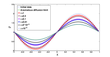
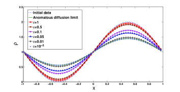
Figure 1: The densities $\rho(T=0.1,x)$ for the micro-macro schemes and the anomalous diffusion limit scheme. Left: the case of heavy-tailed equilibrium. Right: the case of degenerate collision frequency.

3 Duhamel formulation based scheme

In this section, our goal is to derive numerical schemes for (1) which go beyond the AP property. More precisely, our aim to construct numerical schemes whose accuracy in time is uniform with respect to $\varepsilon$. Note that although the scheme of the last section is AP, it does not enjoy this uniform accuracy property (see [3]). The starting point of the derivation is a Duhamel formulation of (1) in Fourier variable, which leads, after an integration in $v$ against $\nu$, to an exact equation on $\hat{\rho}_{\nu}$

$$\hat{\rho}_{\nu}(t,k)=\hat{A}_{0}(t,k)+(\left\langle\nu(v)M\right\rangle)^{-1}\int_{0}^{\frac{t}{\varepsilon^{\alpha}}}\left\langle\mathrm{e}^{-s(\nu(v)+\mathrm{i}\varepsilon k\cdot v)}\nu(v)^{2}M(v)\right\rangle\hat{\rho}_{\nu}(t-\varepsilon^{\alpha}s,k)\mathrm{d}s,$$ (8)

with $\hat{A}_{0}(t,k)=\left\langle\mathrm{e}^{-\frac{t}{\varepsilon^{\alpha}}\left(\nu(v)+\mathrm{i}\varepsilon k\cdot v\right)}\nu(v)\hat{f}_{0}(k,v)\right\rangle/\left\langle\nu(v)M\right\rangle$. Considering discrete time values $t_{n}=n\Delta t,0\leq n\leq N,N\Delta t=T,(T,\Delta t>0)$, and evaluating (8) at $t=t_{n+1}$ leads to

$$\hat{\rho}_{\nu}(t_{n+1},k)=\hat{A}_{0}(t_{n+1},k)+(\left\langle\nu(v)M\right\rangle)^{-1}\sum_{j=0}^{n}\int_{\frac{t_{j}}{\varepsilon^{\alpha}}}^{\frac{t_{j+1}}{\varepsilon^{\alpha}}}\left\langle\mathrm{e}^{-s(\nu(v)+\mathrm{i}\varepsilon k\cdot v)}\nu(v)^{2}M(v)\right\rangle\hat{\rho}_{\nu}(t_{n+1}-\varepsilon^{\alpha}s,k)\mathrm{d}s.$$

For $s\in[t_{j}/\varepsilon^{\alpha},t_{j+1}/\varepsilon^{\alpha}]$, using $\hat{\rho}_{\nu}^{n}\sim\hat{\rho}_{\nu}(t_{n})$, we consider the approximation $\rho_{\nu}(t_{n+1}-\varepsilon^{\alpha}s,k)\approx(t_{j+1}-\varepsilon^{\alpha}s)/\Delta t\;\rho_{\nu}^{n+1-j}+(\varepsilon^{\alpha}s-t_{j})/\Delta t\;\rho_{\nu}^{n-j}$ and get the following proposition.

Proposition 3.1

We introduce the Duhamel formulation based scheme defined for all $x\in\mathbb{R}^{d},v\in\mathbb{R}^{d}$ and all time index $0\leq n\leq N,N\Delta t=T$ by

$$\hat{\rho}^{n+1}_{\nu}=\hat{A}_{0}(t^{n+1},k)+\frac{1}{\left\langle\nu(v)M\right\rangle}\sum\limits_{j=0}^{n}(c_{j}-b_{j})\hat{\rho}^{n+1-j}_{\nu}+b_{j}\hat{\rho}^{n-j}_{\nu},$$ (9)

where

$$b_{j} =\int_{\frac{t_{j}}{\varepsilon^{\alpha}}}^{\frac{t_{j+1}}{\varepsilon^{\alpha}}}\frac{\varepsilon^{\alpha}s-t_{j}}{\Delta t}\left\langle\nu(v)^{2}M\mathrm{e}^{-s\nu(v)}\right\rangle\mathrm{d}s+\int_{\frac{t_{j}}{\varepsilon^{\alpha}}}^{\frac{t_{j+1}}{\varepsilon^{\alpha}}}\frac{\varepsilon^{\alpha}s-t_{j}}{\Delta t}\left\langle\nu(v)^{2}M\left(\mathrm{e}^{-s(\nu(v)+\mathrm{i}\varepsilon k\cdot v)}-\mathrm{e}^{-s\nu(v)}\right)\right\rangle\mathrm{d}s,$$ (10)

$$c_{j} =\int_{\frac{t_{j}}{\varepsilon^{\alpha}}}^{\frac{t_{j+1}}{\varepsilon^{\alpha}}}\left\langle\nu(v)^{2}M\mathrm{e}^{-s\nu(v)}\right\rangle\mathrm{d}s+\int_{\frac{t_{j}}{\varepsilon^{\alpha}}}^{\frac{t_{j+1}}{\varepsilon^{\alpha}}}\left\langle\nu(v)^{2}M\left(\mathrm{e}^{-s(\nu(v)+\mathrm{i}\varepsilon k\cdot v)}-\mathrm{e}^{-s\nu(v)}\right)\right\rangle\mathrm{d}s.$$ (11)

This scheme is of order $1$ uniformly in $\varepsilon$: $\exists C>0$ independent from $\varepsilon$, such that $\max_{k}|\hat{\rho}_{\nu}(t^{n},k)-\hat{\rho}_{\nu}^{n}(k)|\leq C\Delta t,\forall 0\leq n\leq N,N\Delta t=T$.

We refer to [3] and [4] for more details and for the proof of the uniform accuracy of this scheme.

The result of this proposition implies in particular, that this semi-discrete scheme enjoys the AP property. Moreover, we will show below how to discretize the velocity integrals in order to preserve this uniform accuracy property for the fully discretized scheme. In fact, as in the previous section, a direct rectangular velocity discretization in (10)-(11) leads to a wrong limit as $\varepsilon$ goes to $0$. Therefore, a change of variable in these velocity integrals is necessary before any discretization to ensure the right anomalous diffusion limit.

In Case $1$ (heavy-tailed equilibrium), we perform the change of variables $w=\varepsilon|k|v$ only in the second velocity bracket of (10) and do the same for (11). Then, a rectangle formula is applied to the obtained integrals. The first velocity bracket in (10) is computed directly using a rectangle formula, and the same is done for (11). We proceed similarly for Case $2$ (degenerate collision frequency), except that we perform the change of variable $w=\varepsilon|k|v/\nu(v)$ at the same places. It is important to note that the discretizations in velocity are independent of $\varepsilon$ and we still have the first order (in time) uniform accuracy with respect to $\varepsilon$; this statement is proved in [4].

In order to highlight the AP character of this scheme, we present in Fig. 2 the densities obtained with the initial data $f_{0}(x,v)=(1+\sin(\pi x))M(v),x\in[-1,1]$ at time $T=0.1$ and with $\Delta t=10^{-2}$. In the case of the heavy-tailed equilibrium, we took $\beta=2.5$ and in the case of the degenerate collision frequency, we took $\beta=0.5$. In both cases, we consider $v_{\text{max}}=5$ and $200$ points of discretization in velocity.

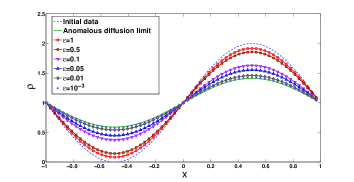
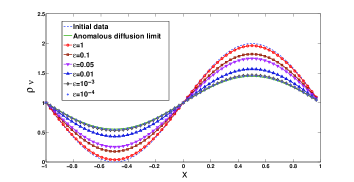
Figure 2: The densities $\rho_{\nu}(T=0.1,x)$ for the Duhamel schemes and the anomalous diffusion limit scheme. Left: the case of heavy-tailed equilibrium. Right: the case of degenerate collision frequency.

Note that in both cases, the distribution function $f$ can be easily recovered from the values of $\rho_{\nu}$ given by the previous scheme, using a Duhamel formulation of the kinetic equation for $f$. The same uniform accuracy property for $f$ is inherited for that of $\rho_{\nu}$.

References

- [1] N. Ben Abdallah, A. Mellet, M. Puel, Anomalous diffusion limit for kinetic equations with degenerate collision frequency. Math. Models Methods Appl. Sci., , , 2011.
- [2] N. Ben Abdallah, A. Mellet, M. Puel, Fractional diffusion limit for collisional kinetic equations: a Hilbert expansion approach. Kinet. Relat. Models, volume , issue , 2011.
- [3] N. Crouseilles, H. Hivert, M. Lemou, Numerical schemes for kinetic equations in the anomalous diffusion limit. Part I: the case of heavy-tailed equilibrium, arXiv: 1503.04586, 2015.
- [4] N. Crouseilles, H. Hivert, M. Lemou, Numerical schemes for kinetic equations in the anomalous diffusion limit. Part II: the case of degenerate collision frequency, in preparation.
- [5] M. Lemou, L. Mieussens, A new asymptotic preserving scheme based on micro-macro formulation for linear kinetic equations in the diffusion limit, SIAM J. Sci. Comput, volume no. , 2008.
- [6] A. Mellet, S. Mischler, C. Mouhot, Fractionnal diffusion limit for collisional kinetic equations, Arch. Ration. Mech. Anal., Vol no., 2011.