Seamless Integration of global Dirichlet-to-Neumann boundary condition and spectral elements for transformation electromagnetics

Abstract.

In this paper, we present an efficient spectral-element method (SEM) for solving general two-dimensional Helmholtz equations in anisotropic media, with particular applications in accurate simulation of polygonal invisibility cloaks, concentrators and circular rotators arisen from the field of transformation electromagnetics (TE). In practice, we adopt a transparent boundary condition (TBC) characterized by the Dirichlet-to-Neumann (DtN) map to reduce wave propagation in an unbounded domain to a bounded domain. We then introduce a semi-analytic technique to integrate the global TBC with local curvilinear elements seamlessly, which is accomplished by using a novel elemental mapping and analytic formulas for evaluating global Fourier coefficients on spectral-element grids exactly.

From the perspective of TE, an invisibility cloak is devised by a singular coordinate transformation of Maxwell’s equations that leads to anisotropic materials coating the cloaked region to render any object inside invisible to observers outside. An important issue resides in the imposition of appropriate conditions at the outer boundary of the cloaked region, i.e., cloaking boundary conditions (CBCs), in order to achieve perfect invisibility. Following the spirit of [48], we propose new CBCs for polygonal invisibility cloaks from the essential “pole” conditions related to singular transformations. This allows for the decoupling of the governing equations of inside and outside the cloaked regions. With this efficient spectral-element solver at our disposal, we can study the interesting phenomena when some defects and lossy or dispersive media are placed in the cloaking layer of an ideal polygonal cloak.

1. Introduction and problem statement

Accurate simulation of wave propagations in inhomogeneous and anisotropic media plays an exceedingly important part in a wide range of applications related to the exploration and design of novel materials that enjoy unusual and remarkable properties in steering waves. In many situations involving time-harmonic wave propagations, the development of high-order methods (i.e., spectral and spectral-element solvers) for the Helmholtz equation and time-harmonic Maxwell equations, is of fundamental importance.

We are concerned with the two-dimensional Helmholtz equation governing time-harmonic wave propagation in anisotropic media:

$$\nabla\cdot\big{(}{\boldsymbol{C}}(\boldsymbol{r})\,\nabla u(\boldsymbol{r})\big{)}+k^{2}n(\boldsymbol{r})u(\boldsymbol{r})=f(\boldsymbol{r}),\quad\boldsymbol{r}=\boldsymbol{x}=(x,y)\in{\mathbb{R}^{2}},$$ (1.1)

where $k>0$ is the wave number in free space. In general, we make the following assumptions.

• $\boldsymbol{C}$ is a symmetric positive definite matrix in ${\mathbb{R}^{2\times 2}},$ and for some positive constants $c_{0},c_{1},$

  $$0<c_{0}\leq\boldsymbol{\xi}^{t}\,\boldsymbol{C}\,\boldsymbol{\xi}\leq c_{1},\;\;\;\forall\,\boldsymbol{\xi}\in{\mathbb{R}}^{2},\;\;\text{a.e. in}\;\;{\mathbb{R}^{2}}.$$ (1.2)

• The coefficient

  $$0<n\leq n_{1},\;\;\;\text{a.e. in}\;\;{\mathbb{R}^{2}}.$$ (1.3)

• The inhomogeneity of the medium is confined in a bounded domain $\Omega_{-}$ with Lipschitz boundary, and $f$ is compactly supported in disc $B_{\!R}$ of radius $R>0$ (see Figure 1.1):

  $${\boldsymbol{C}}={\boldsymbol{I}}_{2},\;\;\;n=1\;\;\;{\rm in}\;\;\;\mathbb{R}^{2}\setminus\bar{\Omega}_{-};\quad{\rm supp}(f)\subseteq B_{\!R},$$ (1.4)

  where $\boldsymbol{I}_{2}$ is the $2\times 2$ identity matrix. In what follows, we are interested in the case where $\Omega_{-}$ is a penetrable scatterer.

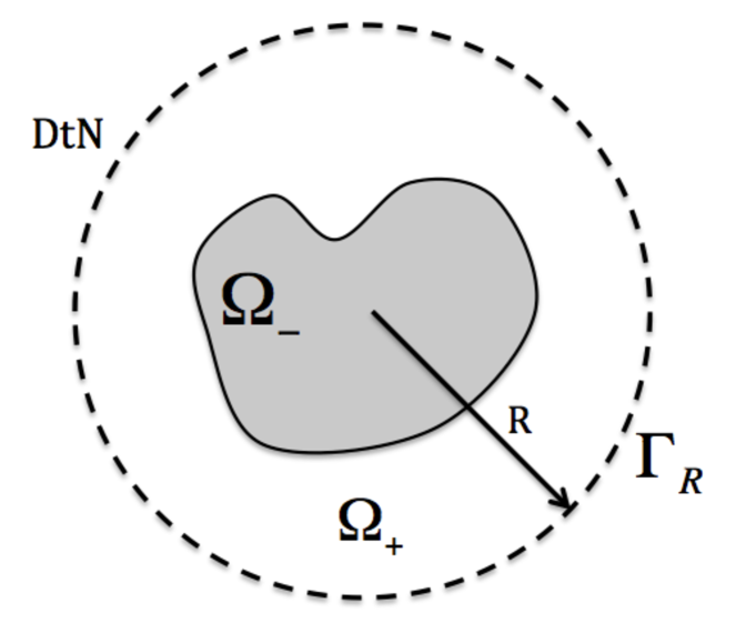
Figure 1.1. Illustration of geometry

We impose the well-known Sommerfeld radiation boundary condition upon the scattering wave: $u_{\rm sc}:=u-u_{\rm in}$ (where $u_{\rm in}$ is a given incident wave):

$$\partial_{r}u_{\rm sc}-{\rm i}k\,u_{\rm sc}=o(r^{-{1}/{2}})\;\;\;{\rm as}\;\;r\rightarrow\infty,$$ (1.5)

where ${\rm i}=\sqrt{-1}$ is the complex unit.  The challenges of the above problem are at least threefold: (i) unboundedness of the computational domain; (ii) indefiniteness of the variational formulation; and (iii) highly oscillatory solution decaying slowly when $k\gg 1.$ In addition, the coefficients ${\boldsymbol{C}}(\boldsymbol{r})$ and $n(\boldsymbol{r})$ might be singular at some interior interface in $\Omega_{-}$ (see Section 3).

The methods of choice to deal with the first issue typically include the perfectly matched layer (PML) technique [5], boundary integral method [22, 30], and the artificial boundary condition [18, 13, 17, 33]. The latter is known as the absorbing boundary condition (ABC), if it leads to a well-posed initial-boundary value problem (IBVP) and some “energy” can be absorbed at the boundary. In particular, if the solution of the reduced problem coincides with that of the original problem, then the related ABC is dubbed as a transparent (or nonreflecting) boundary condition (TBC) (or NRBC). In this paper, we adopt the exact TBC (see [33] and Figure 1.1):

$$\partial_{r}u_{\rm sc}-\mathscr{T}_{R}[u_{\rm sc}]=0\quad{\rm at}\;\;\Gamma_{\!R},$$ (1.6)

where the DtN map $\mathscr{T}_{R}$ is defined as

$${\mathscr{T}}_{R}[\psi]=\sum_{|m|=0}^{\infty}\mathcal{T}_{m}\hat{\psi}_{m}e^{{\rm i}m\theta},\quad{\rm with}$$ (1.7)

$$\hat{\psi}_{m}=\frac{1}{2\pi}\int_{0}^{2\pi}\psi(R,\theta)e^{-{\rm i}m\theta}{\rm d}\theta,\quad{\mathcal{T}}_{m}:=\frac{k{H_{m}^{(1)}}^{\prime}(kR)}{H_{m}^{(1)}(kR)}.$$ (1.8)

Here, $H_{m}^{(1)}(z)$ is the Hankel function of the first kind (cf. [1]). This yields the exact boundary condition for the total field:

$$\partial_{r}u-{\mathscr{T}}_{R}[u]=\partial_{r}u_{\rm in}-{\mathscr{T}}_{R}[u_{\rm in}]:=h\quad{\rm at}\;\;\Gamma_{\!R}.$$ (1.9)

We find it is advantageous to impose DtN TBC for the following reasons.

• The original problem in ${\mathbb{R}}^{2}$ reduces to an equivalent boundary value problem (BVP) in $B_{\!R}.$ One can place $\Gamma_{\!R}$ as close as possible to $\Omega_{-},$ as long as the inhomogeneity of the media and support of the source term are confined in $B_{\!R}.$

• It is essential for accurate and stable simulations especially when the wavenumber is large.

However, the TBC (1.9) is global in space, that is, evaluating ${\mathscr{T}}_{R}[u](x)$ at any point $x_{0}\in\Gamma_{\!R}$ requires to compute the global Fourier integral along the circle $\Gamma_{\!R}.$ This poses challenges in solving the reduced Helmholtz problem by a local element-based method.

• The spectral-element solution (using curvilinear elements along $\Gamma_{\!R}$) is piecewise continuous (i.e., only in $C^{0}(\Gamma_{\!R})$), and defined on spectral-element grids, so the interplay between Fourier points and spectral-element grids via interpolation and fast Fourier transform (FFT) only leads to a first-order convergence.

• One can evaluate the Fourier integral by a composite rule with a decomposition coherent to the spectral-element partition, but due to the elemental mapping between the curvilinear element and reference square, a numerical quadrature is usually necessary, which is prohibitive as the integrands are highly oscillatory for high Fourier modes (see (2.28)).

One main purpose of this paper is to seamlessly integrate the global DtN BC with local spectral elements. The key idea is to construct a new elemental mapping between the curvilinear elements along $\Gamma_{\!R}$ and the reference square (see Figure 2.1), which leads to exact evaluation of the Fourier integrals. It is noteworthy that Fournier [14] proposed a method for calculating global Fourier coefficients for given nodal values on non-conforming spectral elements, where a similar semi-analytic approach was essential for the success of the method therein. We also remark that the recent work [19] addressed the integration of one-dimensional DtN TBC imposed on a line segment with standard rectangular elements along the boundary. Different from these works, our “local-to-global” method is built upon the use of curvilinear elements seamlessly fitting the circular boundary, and the design of a new elemental mapping leading to exact calculation of the involved Fourier integrals (see Subsection 2.3.2).

Underpinned by the advent of metamaterials, transformation electromagnetics (TE) (cf. [36, 27]) provides a powerful tool for creating novel devices and new materials with unconventional properties (see, e.g., [46, 39, 8, 10, 47, 38] and [44] for many original references therein). Some exciting applications of TE include the invisibility cloaks (see, e.g., [36, 16]), rotators (see, e.g., [8]) and concentrators (see, e.g., [39]), which naturally give rise to the model problem (1.1)-(1.5). In particular, the invisibility cloak is devised by a singular coordinate transformation [36] that leads to singular materials coating the cloaked regions and preventing waves from penetrating into the inside region. The imposition of appropriate interface conditions at the inner boundary, i.e., CBCs, where the material parameters are singular, becomes critical. Significant efforts have been devoted to CBCs for circular cylindrical and spherical cloaks. Ruan et al. [41] first analytically studied the sensitivity of the ideal circular cloak [36] to a small $\delta$-perturbation of the inner boundary. Zhang et al. [50] provided deep insights into the physical effects of the singular transformation (also see [49]). To shield the incoming waves, the perfect magnetic conductor (PMC) condition was imposed at the inner boundary in finite-element simulations (see, e.g., [11, 28, 31]). Weder [43] proposed CBCs for the ideal spherical cloak of Pendry et al. [36] from the perspective of energy conservation. Lassas and Zhou [26, 25] proposed some non-local pesudo-differential CBCs. Based upon the principle that a well-behaved electromagnetic field in the original space must be well-behaved in the transformed space as well, Yang and Wang [48] obtained CBCs for circular and elliptical cloaks that intrinsically relate to the essential “pole” conditions of a singular transformation.

The polygonal cloaks enjoy more flexibility to hide objects with complex shapes, which are however much less studied. Indeed, many of the previous principles and approaches for CBCs are not extendable to the polygonal case. Following the spirit of [48], we propose new CBCs under a “local” coordinate system (see Proposition 3.1), under which the governing equation in the cloaked region is decoupled from the exterior region. Accordingly, no wave can propagate into the cloaked region, and vice versa. We emphasise that the new CBCs are indispensable for spectrally accurate simulations. We also show that the proposed spectral-element solver provides a reliable tool to study how the defects affect the perfectness of an ideal cloak (see Subsection 3.5).

The rest of the paper is organised as follows. In Section 2, we review the form invariant of Maxwell equations and illustrate the derivation of the above model problem. We then introduce the technique to seamlessly integrate the global DtN BC with local spectral elements. Section 3 is for accurate simulation of polygonal invisibility cloak, where new CBCs are derived and efficient techniques are introduced to deal with singular material parameters. Various numerical results are provided to show the perfectness of invisibility, and the effects of defects and lossy or dispersive media. Section 4 concerns the extension of the spectral-element solver to the simulation of electromagnetic concentrators and rotators.

2. TE and spectral-element discretization of DtN BC

In this section, we first illustrate the scenarios of the aforementioned model Helmholtz problem arisen from transformation electromagnetics. We then discretise the model problem by spectral-element method and focus on how to seamlessly integrate the global DtN BC with local elements.

2.1. Form invariant of Maxwell equations

Consider the time-harmonic Maxwell system:

$$\breve{\nabla}_{\!\breve{\boldsymbol{r}}}\times\breve{\boldsymbol{E}}-{\rm i}\omega\mu_{0}\,\breve{\boldsymbol{H}}=\boldsymbol{0},\quad\nabla_{\!\breve{\boldsymbol{r}}}\times\breve{\boldsymbol{H}}+{\rm i}\omega\epsilon_{0}\,\breve{\boldsymbol{E}}=\boldsymbol{0},$$ (2.1)

in Cartesian coordinates: $\breve{\boldsymbol{r}}=\breve{\boldsymbol{x}}=(\breve{x},\breve{y},\breve{z})\in{\mathbb{R}}^{3},$ where the electric permittivity $\epsilon_{0},$ the magnetic permeability $\mu_{0},$ and the angular frequency $\omega$ are positive constants. Note that $e^{-{\rm i}\omega t}$ time-dependence is assumed for the electric and magnetic fields.

A remarkable property of the Maxwell system is its form invariant under any coordinate transformation (cf. [37]). More precisely, given a coordinate transformation $\boldsymbol{r}=\boldsymbol{r}(\breve{\boldsymbol{r}})$ with the Jacobian matrix $\boldsymbol{J}=\partial{\boldsymbol{r}}/\partial{\breve{\boldsymbol{r}}},$ the transformed Maxwell system takes the same form:

$$\nabla\times{\boldsymbol{E}}-{\rm i}\omega\mu_{0}{\boldsymbol{\mu}}\,{\boldsymbol{H}}=\boldsymbol{0},\quad\nabla\times{\boldsymbol{H}}+{\rm i}\omega\epsilon_{0}{\boldsymbol{\epsilon}}\,{\boldsymbol{E}}=\boldsymbol{0},$$ (2.2)

where $\nabla\times$ is the curl operator in the new coordinates, and

$$\boldsymbol{E}(\boldsymbol{r})=(\boldsymbol{J}^{t})^{-1}\breve{\boldsymbol{E}}(\breve{\boldsymbol{r}}),\quad\boldsymbol{H}(\boldsymbol{r})=(\boldsymbol{J}^{t})^{-1}\breve{\boldsymbol{H}}(\breve{\boldsymbol{r}}),\quad{\boldsymbol{\mu}}={\boldsymbol{\epsilon}}={\boldsymbol{J}\boldsymbol{J}^{t}}\big{/}{{\rm det}({\boldsymbol{J}})}.$$ (2.3)

We are concerned with the two-dimensional electromagnetic wave propagations in media with in-plane anisotropy. Accordingly, under the transverse-electric (TE) polarization, we consider ${\boldsymbol{E}}=(0,0,u(x,y))^{t}$ and $\boldsymbol{H}=(H_{1},H_{2},0)^{t}$. Letting $z=\breve{z}$ in the coordinate transformation, the material parameters in (2.3) reduce to

$${\boldsymbol{\mu}}={\boldsymbol{\epsilon}}=\begin{bmatrix}{\boldsymbol{C}}&\boldsymbol{0}^{t}\\[2.0pt] \boldsymbol{0}&n\end{bmatrix}=\begin{bmatrix}C_{11}&C_{12}&0\\[1.0pt] C_{12}&C_{22}&0\\[1.0pt] 0&0&n\end{bmatrix},$$ (2.4)

where

$${\boldsymbol{C}}=\frac{\boldsymbol{J}_{\!{\rm cn}}\,\boldsymbol{J}^{t}_{\!{\rm cn}}}{{\rm det}(\boldsymbol{J}_{\!{\rm cn}})},\quad n=\frac{1}{{\rm det}(\boldsymbol{J}_{\!{\rm cn}})}\;\;\;{\rm with}\;\;\;\boldsymbol{J}_{\!{\rm cn}}:=\begin{bmatrix}\partial_{\breve{x}}x&\partial_{\breve{y}}x\\[1.0pt] \partial_{\breve{x}}y&\partial_{\breve{y}}y\\[1.0pt] \end{bmatrix}.$$ (2.5)

Note that ${\rm det}(\boldsymbol{C})=1,$ and

$${\boldsymbol{\mu}}^{-1}={\boldsymbol{\epsilon}}^{-1}=\begin{bmatrix}C_{22}&-C_{12}&0\\[1.0pt] -C_{12}&C_{11}&0\\[1.0pt] 0&0&n^{-1}\end{bmatrix}.$$ (2.6)

Then we derive from the first equation of (2.2) and (2.6) that

$$\begin{split}{\boldsymbol{H}}&=\frac{{\boldsymbol{\mu}}^{-1}}{{\rm i}\omega\mu_{0}}\nabla\times{\boldsymbol{E}}=\frac{{\boldsymbol{\mu}}^{-1}}{{\rm i}\omega\mu_{0}}\big{(}u_{y},-u_{x},0\big{)}^{t}=\frac{1}{{\rm i}\omega\mu_{0}}\big{(}C_{12}u_{x}+C_{22}u_{y},-C_{11}u_{x}-C_{12}u_{y},0\big{)}^{t}.\end{split}$$ (2.7)

Inserting it into the second equation of (2.2), we obtain the two-dimensional Helmholtz equation:

$$\nabla\cdot({\boldsymbol{C}}(\boldsymbol{r})\;\nabla u(\boldsymbol{r}))+k^{2}n(\boldsymbol{r})\,u(\boldsymbol{r})=0,$$ (2.8)

where $k=\omega\sqrt{\epsilon_{0}\mu_{0}}$ is the wavenumber in free space.

In Sections 3-4, we shall introduce the coordinate transformations for polygonal invisibility cloaks, concentrators and rotators, and compute the corresponding material parameters $\boldsymbol{C}$ and $n$ via (2.5). It is noteworthy that in all cases, the coordinate transformations are identity in ${\mathbb{R}}^{2}\setminus(\Omega_{-}\cup\Omega_{+})$ (cf. Figure 1.1), so (1.4) can be met. Moreover, we can derive (2.12) below from the standard transmission conditions (see, e.g., [35, Sec. 1.5] and [32]), that is, the continuity of the tangential components of $\boldsymbol{E}$ and $\boldsymbol{H}$ at the interface $\Gamma:=\partial\Omega_{-}.$

In summary, the problem of interest reads

$$\nabla\cdot({\boldsymbol{C}}(\boldsymbol{r})\nabla u(\boldsymbol{r}))+k^{2}n(\boldsymbol{r})u(\boldsymbol{r})=f(\boldsymbol{r})\quad{\rm in}\;\;B_{R},$$ (2.9)

$$\llbracket u\rrbracket=\llbracket\boldsymbol{C}\,\nabla u\rrbracket=0\;\quad{\rm at}\;\;\Gamma,$$ (2.10)

$$\partial_{r}u-{\mathscr{T}}_{R}[u]=h\qquad{\rm at}\;\;\Gamma_{\!R},$$ (2.11)

where

$$\llbracket u\rrbracket:=u^{-}-u^{+},\quad\llbracket\boldsymbol{C}\,\nabla u\rrbracket:={\boldsymbol{n}}\cdot({\boldsymbol{C}}^{-}\nabla u^{-}-\boldsymbol{C}^{+}\nabla u^{+}),$$ (2.12)

$u^{\pm}:=u|_{\Omega_{\pm}},$ $\boldsymbol{C}^{\pm}:=\boldsymbol{C}|_{\Omega_{\pm}}$ and $\boldsymbol{n}$ is the unit outer normal vector along $\Gamma.$

2.2. Spectral-element scheme

Let $\Omega$ be a generic bounded domain, and $L^{2}(\Omega)$ be the space of square integrable functions with the inner product and norm denoted by $(\cdot,\cdot)_{\Omega}$ and $\|\cdot\|_{\Omega}$ as usual. The Sobolev space $H^{m}(\Omega)$ with $m>0$ is defined as in Admas [2] with the normal $\|u\|_{m,\Omega}.$ Define the trace integral

$$\langle u,v\rangle_{\Gamma_{\!R}}:=\oint_{\Gamma_{\!R}}u\,\bar{v}\,{\rm d}\gamma.$$ (2.13)

A weak formulation of (2.9)-(2.11) is to find $u\in H^{1}(B_{\!R})$ such that

$$\begin{split}\mathscr{B}(u,v):&=({\boldsymbol{C}}\,\nabla u,\nabla v)_{B_{\!R}}-k^{2}(nu,v)_{B_{\!R}}-\langle{\mathscr{T}}_{R}[u],v\rangle_{\Gamma_{\!R}}\\ &=\mathscr{F}(v):=-(f,v)_{B_{\!R}}+\langle h,v\rangle_{\Gamma_{\!R}},\quad\forall v\in H^{1}(B_{\!R}),\end{split}$$ (2.14)

where by (1.7)-(1.8),

$$\langle{\mathscr{T}}_{R}[u],v\rangle_{\Gamma_{\!R}}=\frac{R}{2\pi}\sum_{|m|=0}^{\infty}\mathcal{T}_{m}\Big{(}\int_{0}^{2\pi}u(R,\theta)e^{-{\rm i}m\theta}{\rm d}\theta\Big{)}\Big{(}\overline{\int_{0}^{2\pi}v(R,\theta)e^{-{\rm i}m\theta}{\rm d}\theta}\Big{)}.$$ (2.15)

Remark 2.1.

Recall that (cf. [33, P. 87])

$$-\frac{|m|+1}{R}\leq{\rm Re}(\mathcal{T}_{m})\leq\frac{1}{R},\quad 0<{\rm Im}(\mathcal{T}_{m})\leq k,\;\;\;|m|=0,1,\cdots.$$ (2.16)

We can claim the unique solvability of (2.14) from (1.2)-(1.4) and (2.16) (cf. [33]). ∎

For simplicity, we assume that the scatterer $\Omega_{-}$ is a polygonal domain or a disk, though our approach is extendable to more complicated domain. We partition the computational domain $B_{\!R}$ into a finite number of non-overlapping straight-sided or curvilinear quadrilateral elements $\{\Omega^{e}\}_{e=1}^{E},$ such that the inner interfaces are aligned with the “edges” of the elements. In particular, we have

$$\Gamma_{\!R}=\bigcup_{e=1}^{E_{R}}\Gamma_{\!\!R}^{e}=\bigcup_{e=1}^{E_{R}}\big{[}\theta_{e},\theta_{e+1}\big{]}=[0,2\pi],\quad r=R,$$ (2.17)

where $\Gamma_{\!\!R}^{e}:=\Gamma_{\!R}\cap\bar{\Omega}^{e}\not=\emptyset$ for all $e\in\{1,\cdots,E\},$ and $\theta_{1}=\theta_{E_{R}+1}$ (see Figure 2.1 (a)). Let $\boldsymbol{\chi}^{e}:Q:=(-1,1)^{2}\to\Omega^{e}$ be a one-to-one elemental mapping defined by

$$\boldsymbol{r}={\boldsymbol{x}}=(x,y)=\boldsymbol{\chi}^{e}(\xi,\eta):=\big{(}\chi^{e}_{1}(\xi,\eta),\chi^{e}_{2}(\xi,\eta)\big{)},\quad\forall\,(\xi,\eta)\in Q.$$ (2.18)

Recall that one commonly-used elemental mapping, originally proposed by Gordon and Hall [15], transforms $Q$ to any quadrilateral $\Omega^{e}$ with straight or curved sides (see, e.g., [12, 6]). Here, we shall use a special Gordon and Hall transform in (2.23)-(2.24) below.

Denote by $\mathcal{P}_{N}$ the set of all polynomials of degree at most $N$ in $[-1,1].$ Introduce the spectral-element solution space

$$V_{N}^{E}:=\big{\{}v\in C(B_{\!R})\,:\,v(\boldsymbol{x})|_{\Omega^{e}}=v(\boldsymbol{\chi}^{e})\in{\mathcal{P}}_{N}^{2},\;1\leq e\leq E\big{\}}.$$ (2.19)

The spectral-element approximation of (2.14) is to find $u_{N}^{E}\in V_{N}^{E}$ such that

$$\mathscr{B}(u_{N}^{E},v_{N}^{E})=\mathscr{F}(v_{N}^{E}),\quad\forall\,v_{N}^{E}\in V_{N}^{E}.$$ (2.20)

In view of Remark 2.1, we can show the well-posedness of (2.20) as with (2.14).

2.3. Seamless integration of SEM with DtN TBC

As usual, the continuous inner product $(\cdot,\cdot)_{\Omega}$ can be evaluated by element-wise discrete inner product based on tensorial Legendre-Gauss-Lobatto (LGL) quadrature, and likewise for the term $\langle h,v_{N}^{E}\rangle_{\Gamma_{\!R}}$ (see, e.g., [12]). However, much care is needed to deal with the term $\langle{\mathscr{T}}_{R}[u_{N}^{E}],v_{N}^{E}\rangle_{\Gamma_{\!R}},$ as the DtN operator is global, but the spectral-element solution is piecewise. One can evaluate (2.27) by using the fast Fourier transform (FFT), but this requires an intermediate interpolation to interplay between spectral-element grids and Fourier points. Since $u_{N}^{E}|_{\Gamma_{\!R}}\in C^{0},$ a naive interpolation only results in a first-order convergence.

In what follows, we introduce an efficient semi-analytical means to compute $\langle{\mathscr{T}}_{R}[u_{N}^{E}],v_{N}^{E}\rangle_{\Gamma_{\!R}}.$ Let $\{\xi_{j}=\eta_{j}\}_{j=0}^{N}$ (in ascending order) be the LGL points in $[-1,1],$ and let $\{l_{j}\}_{j=0}^{N}$ be the associated Lagrange interpolating basis polynomials. Correspondingly, the spectral-element grids and basis on $\bar{\Omega}^{e}$ are given by

$$\boldsymbol{x}_{ij}=\boldsymbol{\chi}^{e}(\xi_{i},\eta_{j}),\quad\psi_{ij}(\boldsymbol{x})=l_{i}(\xi)l_{j}(\eta),\quad 0\leq i,j\leq N.$$ (2.21)

Formally, we can write

$$u_{N}^{E}(x,y)\big{|}_{\Omega^{e}}=\sum_{i,j}\tilde{u}_{ij}^{e}\,l_{i}(\xi)l_{j}(\eta),$$ (2.22)

where the unknowns $\{\tilde{u}_{ij}^{e}\}$ are determined by the scheme (2.20).

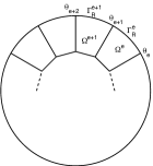
(a) Curvilinear elements

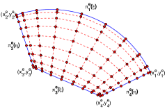
(b) Mapped LGL points on $\Omega^{e}$

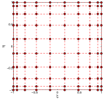
(c) LGL points on $Q$

Figure 2.1. Curvilinear elements and tensorial LGL points on the reference square and a curvilinear element via the new elemental mapping.

We now particularly look at the Gordon-Hall transform for a curvilinear element $\Omega^{e}$ with vertices $\{(x_{i}^{e},y_{i}^{e})\}_{i=1}^{4}$ along $\Gamma_{\!R}$ (with three straight sides). Let $\{\boldsymbol{\pi}_{j}^{e}(t),t\in[-1,1]\}_{j=1}^{4}$ be, respectively, the parametric form of four sides such that

$$\boldsymbol{\pi}_{1}^{e}(-1)=\boldsymbol{\pi}_{4}^{e}(1),\;\;\boldsymbol{\pi}_{1}^{e}(1)=\boldsymbol{\pi}_{2}^{e}(1),\;\;\boldsymbol{\pi}_{2}^{e}(-1)=\boldsymbol{\pi}_{3}^{e}(1),\;\;\boldsymbol{\pi}_{3}^{e}(-1)=\boldsymbol{\pi}_{4}^{e}(-1),$$ (2.23)

see Figure 2.1 (b). In this case, the Gordon-Hall transform takes the form

$$\begin{split}{\boldsymbol{x}}={\boldsymbol{\chi}}^{e}(\xi,\eta)=&{\boldsymbol{\pi}}_{1}^{e}(\xi)\frac{1+\eta}{2}+{\boldsymbol{\pi}}_{3}^{e}(\xi)\frac{1-\eta}{2}+\frac{1+\xi}{2}{\boldsymbol{\pi}}_{2}^{e}(\eta)+\frac{1-\xi}{2}{\boldsymbol{\pi}}_{4}^{e}(\eta)\\ &-\bigg{(}{\boldsymbol{\pi}}_{1}^{e}(-1)\frac{1-\xi}{2}+{\boldsymbol{\pi}}_{1}^{e}(1)\frac{1+\xi}{2}\bigg{)}\frac{1+\eta}{2}\\ &-\bigg{(}{\boldsymbol{\pi}}_{3}^{e}(-1)\frac{1-\xi}{2}+{\boldsymbol{\pi}}_{3}^{e}(1)\frac{1+\xi}{2}\bigg{)}\frac{1-\eta}{2}\,,\end{split}$$ (2.24)

where the edge $\eta=1$ of $Q$ is mapped to the arc $\Gamma_{\!\!R}^{e}=\{r=R,\;\theta\in(\theta_{e},\theta_{e+1})\}$ of $\Omega_{e},$ i.e.,

$$\Gamma^{e}_{\!R}\,:\,\;x=\chi_{1}^{e}(\xi,1)=\pi_{11}^{e}(\xi),\;\;y=\chi_{2}^{e}(\xi,1)=\pi_{12}^{e}(\xi),\quad\forall\,\xi\in(-1,1).$$ (2.25)

Accordingly, the spectral-element grids in polar coordinates on $\Gamma_{\!\!R}^{e}$ (see Figure 2.1) satisfy

$$\cos\theta_{j}^{e}=R^{-1}{\pi_{11}^{e}(\xi_{j})}\;\;{\rm or}\;\;\sin\theta_{j}^{e}=R^{-1}{\pi_{12}^{e}(\xi_{j})},\quad 1\leq j\leq N.$$ (2.26)

We now turn to $\langle{\mathscr{T}}_{R}[u_{N}^{E}],v_{N}^{E}\rangle_{\Gamma_{\!R}}$ in (2.20). Thanks to (2.15) and (2.22), we need to evaluate

$$\begin{split}\int_{0}^{2\pi}u_{N}^{E}(x,y)\big{|}_{\Gamma_{\!R}}e^{-{\rm i}m\theta}\,{\rm d}\theta&=\sum_{e=1}^{E_{R}}\int_{\theta_{e}}^{\theta_{e+1}}u_{N}^{E}(x,y)\big{|}_{\Gamma_{\!R}^{e}}e^{-{\rm i}m\theta}\,{\rm d}\theta\\ &=\sum_{e=1}^{E_{R}}\sum_{i}\tilde{u}_{iN}^{e}\int_{-1}^{1}l_{i}(\xi)e^{-{\rm i}m\theta(\xi)}\frac{{\rm d}\theta}{{\rm d}\xi}\,{{\rm d}\xi}.\end{split}$$ (2.27)

As the nodal basis $\{l_{i}\}$ can be represented in terms of Legendre polynomials, it suffices to compute

$${\mathbb{I}}_{nm}^{e}:=\int_{-1}^{1}P_{n}(\xi)\,e^{-{\rm i}m\theta(\xi)}\,\frac{{\rm d}\theta}{{\rm d}\xi}\,{\rm d}\xi,\;\;\;\;{\rm for}\;\;n\geq 0,\;\;|m|\geq 0,$$ (2.28)

where $P_{n}$ is the Legendre polynomial of degree $n$, and by (2.25),

$$\frac{{\rm d}\theta}{{\rm d}\xi}=\frac{1}{R}\frac{{\rm d}\gamma}{{\rm d}\xi}=R^{-1}\sqrt{\big{[}\partial_{\xi}\pi_{11}^{e}(\xi)\big{]}^{2}+\big{[}\partial_{\xi}\pi_{12}^{e}(\xi)\big{]}^{2}}\,.$$ (2.29)

It is seen that the integrand is highly oscillatory for large $|m|,$ and the efficiency and accuracy in computing ${\mathbb{I}}_{nm}^{e}$ essentially relies on the choice of the parametric form for $\boldsymbol{\pi}_{1}(\xi).$ We next introduce a parametric form that allows for exact evaluation of (2.29) by analytic formulas (see Propositions 2.1-2.2). To stimulate the idea, we first consider a commonly-used parametric form.

2.3.1. A commonly-used parametric form for $\boldsymbol{\pi}^{e}_{1}(\xi)$

Following the ideas of the cubed-sphere transformation (cf. [40, 52]) and the “ray” coordinates (cf. [23]), one can project the secant line: $(x_{1}^{e},y_{1}^{e})$, $(x_{2}^{e},y_{2}^{e})$ to the arc $\Gamma^{e}_{\!R}$ via the “rays” from the origin. This leads to the parameterisation:

$$\boldsymbol{\pi}^{e}_{1}(\xi)=(\pi^{e}_{11}(\xi),\pi^{e}_{12}(\xi))=\bigg{(}\frac{R\,d_{1}(\xi)}{\sqrt{d_{1}^{2}(\xi)+d^{2}_{2}(\xi)}},\frac{R\,d_{2}(\xi)}{\sqrt{d_{1}^{2}(\xi)+d^{2}_{2}(\xi)}}\bigg{)},$$ (2.30)

where

$$d_{1}(\xi)=\frac{x_{2}^{e}-x_{1}^{e}}{2}\xi+\frac{x_{1}^{e}+x_{2}^{e}}{2},\quad d_{2}(\xi)=\frac{y_{2}^{e}-y_{1}^{e}}{2}\xi+\frac{y_{1}^{e}+y_{2}^{e}}{2}.$$ (2.31)

Since $\cos\theta=R^{-1}\pi_{11}^{e}(\xi),$ we find

$$\theta(\xi)=\begin{cases}\alpha,\quad&{\rm if}\;\;\;\theta\in[0,\pi),\\[4.0pt] 2\pi-\alpha,\quad&{\rm if}\;\;\;\theta\in[\pi,2\pi),\end{cases}\quad\alpha:=\cos^{-1}\bigg{(}\frac{d_{1}(\xi)}{\sqrt{d_{1}^{2}(\xi)+d^{2}_{2}(\xi)}}\bigg{)}\,,$$ (2.32)

and (2.29) reads

$$\frac{{\rm d}\theta}{{\rm d}\xi}=\frac{|x_{1}^{e}y_{2}^{e}-x_{2}^{e}y_{1}^{e}|}{2(d_{1}^{2}(\xi)+d^{2}_{2}(\xi))},\quad\forall\,\xi\in[-1,1].$$ (2.33)

Inserting (2.32) and (2.33) into (2.28), one immediately finds that ${\mathbb{I}}_{nm}^{e}$ appears complicated and must be evaluated numerically. However, the integrand is highly oscillatory, when $|m|$ is large.

2.3.2. A new parametric form for $\boldsymbol{\pi}^{e}_{1}(\xi)$

We next take a very different route to parameterise $\Gamma^{e}_{\!R}.$ The essential idea is to look for

$$\boldsymbol{\pi}^{e}_{1}(\xi)=\big{(}\pi_{11}^{e}(\xi),\pi_{12}^{e}(\xi)\big{)}=R(\cos\theta,\sin\theta),\quad\theta\in[\theta_{e},\theta_{e+1}],\;\;\xi\in[-1,1],$$ (2.34)

such that ${\rm d}{\gamma}=a\,{\rm d}\xi,$ that is, the arc length $\gamma$ is linear in $\xi.$

Proposition 2.1.

Let $\Omega^{e}$ be the curvilinear element as in Figure 2.1 (b). Then the new elemental mapping from the reference square $Q$ to $\Omega^{e}$ takes the form

$$x =\pi_{11}^{e}(\xi)\frac{1+\eta}{2}+\frac{(1+\xi)(1-\eta)}{4}x_{3}^{e}+\frac{(1-\xi)(1-\eta)}{4}x_{4}^{e},$$ (2.35)

$$y =\pi_{12}^{e}(\xi)\frac{1+\eta}{2}+\frac{(1+\xi)(1-\eta)}{4}y_{3}^{e}+\frac{(1-\xi)(1-\eta)}{4}y_{4}^{e},$$ (2.36)

where

$$\boldsymbol{\pi}^{e}_{1}(\xi)=\big{(}\pi_{11}^{e}(\xi),\pi_{12}^{e}(\xi)\big{)}=R\big{(}\cos(\hat{\theta}_{e}\xi+\beta_{e}),\sin(\hat{\theta}_{e}\xi+\beta_{e})\big{)},$$ (2.37)

with

$$\hat{\theta}_{e}=\frac{\theta_{e+1}-\theta_{e}}{2},\quad\beta_{e}=\frac{\theta_{e}+\theta_{e+1}}{2}.$$ (2.38)

Proof.

Let $\gamma=a\xi+b.$ The arc length along $\Gamma_{\!R}^{e}$ is $\gamma=R(\theta-\theta_{e}),$ so we have

$$a\xi+b=R(\theta-\theta_{e}).$$ (2.39)

Since $\theta=\theta_{e}$ (resp. $\theta=\theta_{e+1}$) is mapped to $\xi=-1$ (resp. $\xi=1$), we find

$$a=b=\hat{\theta}_{e}R,\quad\theta=\hat{\theta}_{e}\xi+\beta_{e},\quad\xi\in[-1,1].$$ (2.40)

Inserting it into (2.34) leads to the new parametric form (2.37). Then we obtain (2.35)-(2.36) from the equations of the straight sides, e.g.,

$$\boldsymbol{\pi}_{4}^{e}(\eta)=\frac{\boldsymbol{x}_{1}^{e}-\boldsymbol{x}_{4}^{e}}{2}\eta+\frac{\boldsymbol{x}_{1}^{e}+\boldsymbol{x}_{4}^{e}}{2},\quad\eta\in[-1,1],$$ (2.41)

and the Gordon-Hall transform (2.24). ∎

Observe that in distinctive contrast to (2.32)-(2.33), the new transformation has a linear dependence of $\theta$ in $\xi,$ so in (2.28),

$$\theta(\xi)=\hat{\theta}_{e}\xi+\beta_{e},\quad\frac{{\rm d}\theta}{{\rm d}\xi}=\hat{\theta}_{e}.$$ (2.42)

This leads to the following analytic means for computing the integrals of interest.

Proposition 2.2.

Under the new transformation in Proposition 2.1, the integral in (2.28) can be computed by

$$\begin{split}&{\mathbb{I}}_{n0}^{e}=2\hat{\theta}_{e}\delta_{n0};\quad{\mathbb{I}}_{nm}^{e}=\frac{2\hat{\theta}_{e}R}{{\rm i}^{n}}\sqrt{\frac{\pi}{2m\hat{\theta}_{e}}}J_{n+1/2}(m\hat{\theta}_{e})\,e^{-{\rm i}m\beta_{e}},\end{split}$$ (2.43)

and ${\mathbb{I}}_{n,-m}^{e}=({\mathbb{I}}_{nm}^{e})^{*}$ for $n\geq 0$ and $m\geq 1,$ where $J_{n+1/2}$ is the Bessel function of the first kind, and $\hat{\theta},\beta_{e}$ are the same as in (2.38).

Proof.

By (2.28) and (2.42),

$${\mathbb{I}}_{nm}^{e}=\int_{-1}^{1}P_{n}(\xi)\,e^{-{\rm i}m\theta(\xi)}\frac{{\rm d}\theta}{{\rm d}\xi}\,{\rm d}\xi=\hat{\theta}_{e}\,e^{-{\rm i}m\beta_{e}}\int_{-1}^{1}P_{n}(\xi)e^{-{\rm i}m\hat{\theta}_{e}\xi}\,{\rm d}\xi.$$ (2.44)

It is clear that for $m=0,$ we have ${\mathbb{I}}_{00}^{e}=2\hat{\theta}_{e},$ and by the orthogonality of Legendre polynomials, we have ${\mathbb{I}}_{n0}^{e}=0$ when $n\geq 1.$ Moreover, we have ${\mathbb{I}}_{n,-m}^{e}=({\mathbb{I}}_{nm}^{e})^{*},$ so we only need to compute the integrals with $m\geq 1.$ Recall the identity (cf. [3])

$$\int_{-1}^{1}P_{n}(\xi)\,e^{-{\rm i}mx\xi}\,{\rm d}\xi=\frac{1}{{\rm i}^{n}}\sqrt{\frac{2\pi}{mx}}J_{n+1/2}(mx),\quad{\rm for}\;\;mx>0.$$ (2.45)

Thus, (2.43) follows immediately. ∎

2.4. An illustrative numerical example

As a by-product, the new parameterisation provides an efficient means to compute the Fourier coefficients via piecewise Legendre approximation. In a nutshell, we partition $[0,2\pi]$ into $\{[\theta_{e},\theta_{e+1}]\}_{e=1}^{E_{R}},$ and approximate the underlying function on each subinterval by Legendre polynomials using (2.37) so that the analytical formula (2.43) can be applied. Here, we provide an example to illustrate this numerical-analytic approach.

Consider the Fourier expansion of a plane wave (cf. [1, P. 360]):

$$e^{{\rm i}k(x\cos\theta_{0}+y\sin\theta_{0})}=\sum_{|m|=0}^{\infty}\hat{g}_{m}e^{{\rm i}m\theta}\;\;\;{\rm with}\;\;\;\hat{g}_{m}={\rm i}^{m}J_{m}(kR)e^{-{\rm i}m\theta_{0}},$$ (2.46)

for some constant $\theta_{0}$, where $J_{m}$ is the Bessel function of the first kind of order $m$ as before. Let $\hat{g}_{m,N}^{E_{R}}$ be the numerical approximation to $\hat{g}_{m},$ and denote the error ${\rm max}_{|m|\leq M}|\hat{g}_{m}-\hat{g}_{m,N}^{E_{R}}|.$ Note that $\hat{g}_{m}$ decays exponentially as $|m|$ increases. We depict the errors against $N$ (with fixed $E_{R}=4$) in Figure 2.2 (left), and against the number of elements $E_{R}$ (with fixed $N=10$) in Figure 2.2 (right), for $R=1$, $M=20,k=10,20,30$ and $\theta_{0}={\pi}/{4}$. We observe exponential convergence in both cases.

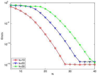
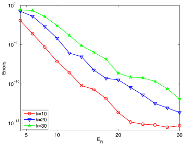
Figure 2.2. Numerical error ${\rm max}_{|m|\leq M}|\hat{g}_{m}-\hat{g}_{m,N}^{E_{R}}|$ with fixed $M=20$, $\theta_{0}={\pi}/{4}$ and $k=10,20,30$. Left: errors against $N$ with $E_{R}=4$. Right: errors against $E_{R}$ with $N=10$.

3. Accurate simulation of polygonal invisibility cloaks

As already mentioned, the invisibility cloak is one of the most exciting examples of transformation electromagnetics outlined in Subsection 2.1. In this section, we apply the spectral-element solver proposed in Section 2 to simulate the polygonal invisibility cloak, and numerically study the effects of defects, lossy media or dispersive media in the cloaking layer. We particularly address the following two important issues.

• How to impose appropriate cloaking boundary conditions at the boundary of the cloaked region to perfectly hide the objects inside the cloaked region?

• How to efficiently treat the singular material parameters in spectral-element discretisation to ensure accurate simulation?

3.1. Coordinate transformation and material parameters

As with Pendry et al. [36], the underlying coordinate transformation for a polygonal cloak blows up the origin $O$ in the original $(\breve{x},\breve{y})$-coordinates in Figure 3.1 (a) to the polygonal domain $\Omega_{-}^{p}=A_{p}B_{p}\cdots F_{p}$ in Figure 3.1 (b), which forms the “cloaked region”. It is expected that the waves from outside can not propagate into $\Omega_{-}^{p}$ so that any object inside is concealed. Accordingly, the polygonal domain $\Omega_{-}$ (i.e., the polygon $AB\cdots F$) is compressed into the polygonal annulus $\Omega_{-}^{a}=\Omega_{-}\setminus\bar{\Omega}_{-}^{p}$, called the “cloaking layer”.

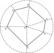
(a) $(\breve{x},\breve{y})$-domain

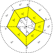
(b) $(x,y)$-domain

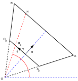
(c) $\boldsymbol{\tau}$ and $\boldsymbol{n}$

Figure 3.1. Schematic geometry of a polygonal cloak. (a) The polygonal domain in the original coordinates $(\breve{x},\breve{y}).$ (b) Through (3.2), the origin is spanned into the polygonal domain $\Omega_{-}^{p}=A_{p}B_{p}\cdots F_{p}$ that forms the cloaked region. Consequently, the original polygonal domain in (a) is compressed into the polygonal annulus $\Omega_{-}^{a}$ (i.e., the shaded part) that forms the cloaking layer. (c) The “local” coordinate system $(\boldsymbol{\tau},\boldsymbol{n}).$

In fact, the coordinate transformations can be best characterised in two polar coordinates as depicted in the diagram:

$${\small\ovalbox{Original: $(\breve{x},\breve{y})$}\xleftarrow{\makebox[8.5359pt]{}}\xrightarrow{\makebox[8.5359pt]{}}\ovalbox{Polar: $(\breve{r},\breve{\theta})$}\xrightarrow{\makebox[51.21504pt]{Transform}}\ovalbox{Polar: $(r,\theta)$}\xleftarrow{\makebox[8.5359pt]{}}\xrightarrow{\makebox[8.5359pt]{}}\ovalbox{Physical: $(x,y)$}}$$ (3.1)

With this, the coordinate transformation for a polygonal cloak takes the form (see, e.g., [53]):

$$\begin{cases}r=(1-\rho)\,\breve{r}+\,R_{1},\quad&\breve{r}\in[0,R_{2}],\;\;\;r\in[R_{1},R_{2}],\\[4.0pt] \theta=\breve{\theta},\quad&\breve{\theta},\theta\in[0,2\pi),\end{cases}$$ (3.2)

where

$$\rho=\frac{OA_{p}}{OA}=\frac{OB_{p}}{OB}=\cdots=\frac{OF_{p}}{OF},\quad 0<\rho<1,$$ (3.3)

and $(R_{1}(\theta),\theta)$ (resp. $(R_{2}(\theta),\theta)$) is the polar parametric form of the side of the cloaked region $\Omega_{-}^{p}$ (resp. the domain $\Omega_{-}$).

We find it is more convenient to introduce a “local” coordinate system to represent $R_{i}$ ($i=1,2$) when we impose the cloaking boundary conditions later on. Consider any side of the insidemost polygonal domain $\Omega_{-}^{p},$ say $A_{p}B_{p}$ in Figure 3.1 (c), with vertices $(x_{1},y_{1})$ and $(x_{2},y_{2}).$ Then its unit tangential vector $\boldsymbol{\tau}$ and unit normal vector $\boldsymbol{n}$ are given by

$${\boldsymbol{\tau}}=\frac{(x_{2}-x_{1},y_{2}-y_{1})}{\sqrt{(x_{2}-x_{1})^{2}+(y_{2}-y_{1})^{2}}}:=(\tau_{1},\tau_{2}),\quad{\boldsymbol{n}}=(\tau_{2},-\tau_{1}),$$ (3.4)

respectively, which form a “local” coordinate system. Noting that for any $(x,y)=(R_{1}\cos\theta,R_{1}\sin\theta)$ along this side, we have $(x,y)\cdot\boldsymbol{n}=(x_{2},y_{2})\cdot\boldsymbol{n}=(x_{1},y_{1})\cdot\boldsymbol{n},$ and

$$R_{1}(\theta)=\frac{\tau_{2}x_{2}-\tau_{1}y_{2}}{\tau_{2}\cos\theta-\tau_{1}\sin\theta},\quad R_{2}(\theta)=\rho^{-1}R_{1}(\theta).$$ (3.5)

We can use (2.5) and (3.2) to derive the coefficients $\boldsymbol{C}$ and $n$ in the Helmholtz equation (2.9). More precisely, the coefficients in $B_{\!R}=\Omega_{-}^{p}\cup\bar{\Omega}_{-}^{a}\cup\Omega_{+}$ take different forms as follows.

• In the cloaking layer $\Omega_{-}^{a}$, the entries of $\boldsymbol{C}$ in (2.4)-(2.5) are given by (see Appendix A):

  $$C_{11} =\frac{r-R_{1}}{r}\frac{x^{2}}{r^{2}}+\frac{1}{r(r-R_{1})}\bigg{(}\frac{{\rm d}R_{1}}{{\rm d}\theta}\frac{x}{r}-y\bigg{)}^{2}\,,$$ (3.6)

  $$C_{22} =\frac{r-R_{1}}{r}\frac{y^{2}}{r^{2}}+\frac{1}{r(r-R_{1})}\bigg{(}\frac{{\rm d}R_{1}}{{\rm d}\theta}\frac{y}{r}+x\bigg{)}^{2}\,,$$ (3.7)

  $$C_{12} =\frac{r-R_{1}}{r}\frac{xy}{r^{2}}+\frac{1}{r(r-R_{1})}\bigg{(}\frac{{\rm d}R_{1}}{{\rm d}\theta}\frac{x}{r}-y\bigg{)}\bigg{(}\frac{{\rm d}R_{1}}{{\rm d}\theta}\frac{y}{r}+x\bigg{)},$$ (3.8)

  and

  $$n=\frac{r-R_{1}}{r(1-\rho)^{2}}\,.$$ (3.9)

• In $\Omega_{+}=B_{R}\setminus\bar{\Omega}_{-}$, we have $\boldsymbol{C}=\boldsymbol{I}_{2}$ and $n=1.$

• Following [36], we set ${\boldsymbol{C}}=\boldsymbol{I}_{2}$ and $n=1$ in $\Omega_{-}^{p}.$

Remark 3.1.

It is seen from (3.5) that $R_{1}$ has a different representation in different trapezoids $\{\Omega_{T}^{i}\}_{i=1}^{6}$ in Figure 3.1 (b), so the entries of $\boldsymbol{C}$ and the coefficient $n$ are piecewise functions, which might be not continuous across the sides in the radial direction, e.g., $A_{p}A$. ∎

3.2. Transmission conditions and new CBCs

For notational convenience, we partition the disk $B_{R}$ into a finite number of non-overlapping subdomains based on the nature of material parameters. Take the setting in Figure 3.1 as an example, and decompose

$$B_{\!R}=\Omega_{-}^{p}\cup\bar{\Omega}_{-}^{a}\cup\Omega_{+},\quad\bar{\Omega}_{-}^{a}=\cup_{i=1}^{6}\bar{\Omega}_{T}^{i},\quad\bar{\Omega}_{+}=\cup_{i=1}^{6}\bar{\Omega}^{i},$$ (3.10)

where $\{\Omega_{T}^{i}\}$ are trapezoids. Denote by $\Gamma_{\!\pm}^{p}$ the “outside” and “inside” boundaries of the cloaked region $\Omega_{-}^{p},$ respectively. We further denote by $\Gamma^{a}:=\bar{\Omega}_{+}\cap\bar{\Omega}_{-}^{a},$ i.e., the outer boundary of $\Omega^{a}.$

We next impose interface conditions: (i) at $\Gamma^{a}$ and sides in the radial direction of the trapezoids $\{\Omega_{T}^{i}\};$ and (ii) at the cloaking boundary $\Gamma_{\!\pm}^{p}.$ In the former case, the material parameters are bounded below and above, so we impose the usual transmission conditions. Recall that under the TE polarisation, $\boldsymbol{E}=(0,0,u)^{t},$ so we have

$$\llbracket u\rrbracket=\llbracket\boldsymbol{C}\nabla u\rrbracket=0\;\quad\text{for case (i)}.$$ (3.11)

In the latter case, the material parameters degenerate at $\Gamma^{p}_{\!+}$ (cf. (3.6)-(3.8)), so the above transmission conditions are not applicable. In fact, the tangential component of $\boldsymbol{E}$ is not continuous across the cloaking boundary. Indeed, it is the singular non-isotropic medium in the cloaking layer $\Omega_{-}^{a}$ that offers the possibility of achieving invisibility within the innermost polygonal domain $\Omega_{-}^{p}$. In practice, the perfect conduct shell, i.e., PEC (under TM polarisation) or PMC (under TE polarisation) was enforced at $\Gamma_{\!+}^{p}$ in simulations (see, e.g., [11] for circular cylindrical cloaks, [21, 24] for elliptic cloaks, [53, 45] for polygonal cloaks, and [54, 29] for time domain cloaks). However, as commented in [11], such a condition was sufficient but not necessary. Indeed, it was shown in [48], the PEC or PMC could not lead to an independent, meaningful boundary condition for circular cylindrical cloaks in polar coordinates.

Following the spirit of [48], we next introduce the essential “pole” conditions associated with the singular transformation (3.2). As we will see, it is important to use the “local” coordinate system $(\boldsymbol{\tau},\boldsymbol{n})$ in (3.4) to decompose the differential operators and then carefully study the singularity.

Proposition 3.1.

Let $(\boldsymbol{\tau},\boldsymbol{n})$ be the “local” coordinate system in (3.4). The CBCs take the form

$$\nabla_{\!\boldsymbol{\tau}}u^{+}=\boldsymbol{\tau}\cdot\nabla u^{+}=0\;\;{\rm at}\;\;\Gamma_{\!+}^{p};\quad\nabla_{\!\boldsymbol{n}}u^{-}=\boldsymbol{n}\cdot\nabla u^{-}=0\;\;{\rm at}\;\;\Gamma_{\!-}^{p},$$ (3.12)

where $u^{+}=u|_{B\setminus\bar{\Omega}_{-}^{p}}$ and $u^{-}=u|_{\bar{\Omega}_{-}^{p}}.$

Proof.

In order to achieve spectral accuracy in simulations involving singular transformations, we follow [48] (also see [42]) and require that the well-behaved and finite electromagnetic fields in the original coordinates $\breve{\boldsymbol{r}}=(\breve{x},\breve{y})$ must be well-behaved and finite in the new coordinates $\boldsymbol{r}=(x,y)$. We therefore apply this principle to the magnetic field in the cloaking layer, and show that the essential “pole” condition of the transformation (3.2) takes the form

$$\nabla_{\!\boldsymbol{\tau}}u^{+}=0\;\;\;\;{\rm at}\;\;\;\Gamma_{\!+}^{p}.$$ (3.13)

Recall that by (2.7), $\boldsymbol{H}^{+}=\boldsymbol{H}|_{B\setminus\bar{\Omega}_{-}^{p}}$ can be expressed as

$${\boldsymbol{H}}^{+}=(H_{1}^{+},H_{2}^{+},0)^{t}=\frac{1}{{\rm i}\omega\mu_{0}}\big{(}C_{12}u_{x}^{+}+C_{22}u_{y}^{+},-C_{11}u_{x}^{+}-C_{12}u_{y}^{+},0\big{)}^{t}.$$ (3.14)

Then we have

$$u_{x}^{+}=\tau_{1}\nabla_{\!\boldsymbol{\tau}}u^{+}-\tau_{2}\nabla_{\!\boldsymbol{n}}u^{+},\quad u_{y}^{+}=\tau_{2}\nabla_{\!\boldsymbol{\tau}}u^{+}+\tau_{1}\nabla_{\!\boldsymbol{n}}u^{+}.$$ (3.15)

Inserting (3.6)-(3.8) and (3.15) into (3.14) and collecting the terms, we obtain

$${\rm i}\omega\mu_{0}H_{1}^{+} =-\Big{(}\frac{r-R_{1}}{r}\tau_{1}+\frac{{\rm d}R_{1}}{{\rm d}\theta}\frac{\tau_{2}}{r}\Big{)}\nabla_{\!\boldsymbol{n}}u^{+}+\frac{{\rm d}R_{1}}{{\rm d}\theta}\frac{\tau_{1}}{r}\nabla_{\!\boldsymbol{\tau}}u^{+}+\frac{\tau_{2}}{r-R_{1}}\Big{(}r+\Big{(}\frac{{\rm d}R_{1}}{{\rm d}\theta}\Big{)}^{2}\frac{1}{r}\Big{)}\nabla_{\!\boldsymbol{\tau}}u^{+},$$ (3.16)

$${\rm i}\omega\mu_{0}H_{2}^{+} =-\Big{(}\frac{r-R_{1}}{r}\tau_{2}-\frac{{\rm d}R_{1}}{{\rm d}\theta}\frac{\tau_{1}}{r}\Big{)}\nabla_{\!\boldsymbol{n}}u^{+}+\frac{{\rm d}R_{1}}{{\rm d}\theta}\frac{\tau_{2}}{r}\nabla_{\!\boldsymbol{\tau}}u^{+}-\frac{\tau_{1}}{r-R_{1}}\Big{(}r+\Big{(}\frac{{\rm d}R_{1}}{{\rm d}\theta}\Big{)}^{2}\frac{1}{r}\Big{)}\nabla_{\!\boldsymbol{\tau}}u^{+}.$$ (3.17)

By (3.5),

$$\frac{{\rm d}R_{1}}{{\rm d}\theta}=R_{1}\dfrac{\tau_{1}x+\tau_{2}y}{\tau_{2}x-\tau_{1}y},$$ (3.18)

which is uniformly bounded in $\bar{\Omega}_{-}^{a}$ (note: $\tau_{2}x-\tau_{1}y=0$ implies the side of the polygonal passes through the origin, which is not possible). Thus, $\boldsymbol{H}^{+}$ is a finite field in $\bar{\Omega}_{-}^{a}$, if and only if the first condition in (3.12) holds.

Let $\boldsymbol{H}^{-}=\boldsymbol{H}|_{\bar{\Omega}_{-}^{p}}.$ From (3.4), (3.6)-(3.8) and (3.14), we obtain

$$\begin{split}\boldsymbol{n}\times\big{(}\boldsymbol{H}^{+}-\boldsymbol{H}^{-}\big{)}\big{|}_{r=R_{1}}&=\frac{1}{{\rm i}\omega\mu_{0}}\big{(}0,0,-\boldsymbol{n}\cdot(\boldsymbol{C}\nabla u^{+})+\nabla_{\boldsymbol{n}}u^{-}\big{)}^{t}\big{|}_{r=R_{1}}\\ &=\frac{1}{{\rm i}\omega\mu_{0}}\Big{(}0,0,-\frac{r-R_{1}}{r}\nabla_{\!\boldsymbol{n}}u^{+}+\frac{1}{r}\frac{dR_{1}}{d\theta}\nabla_{\!\boldsymbol{\tau}}u^{+}+\nabla_{\boldsymbol{n}}u^{-}\Big{)}^{t}\Big{|}_{r=R_{1}},\end{split}$$ (3.19)

where the restriction at $r=R_{1}$ means that we approach the cloaking boundary from the inside and the outside. Suppose that $\nabla_{\boldsymbol{n}}u^{+}$ is finite. Then by (3.13),

$$\boldsymbol{n}\times\big{(}\boldsymbol{H}^{+}-\boldsymbol{H}^{-}\big{)}\big{|}_{r=R_{1}}=\frac{1}{{\rm i}\omega\mu_{0}}\big{(}0,0,\nabla_{\boldsymbol{n}}u^{-}\big{)}^{t}\big{|}_{r=R_{1}}.$$ (3.20)

By imposing the second condition in (3.12), we find

$$\boldsymbol{H}^{-}\times\boldsymbol{n}=\frac{1}{{\rm i}\omega\mu_{0}}\big{(}\nabla\times\boldsymbol{E}^{-}\big{)}\times\boldsymbol{n}=0\quad{\rm at}\;\;\Gamma_{-}^{p},$$ (3.21)

and by (3.19), the tangential component of the magnetic field $\boldsymbol{H}$ is continuous across the cloaking boundary. ∎

Remark 3.2.

Weder [43] proposed CBCs for point-transformed 3D invisibility cloaks:

$$\boldsymbol{E}^{+}\times\boldsymbol{n}=\boldsymbol{H}^{+}\times\boldsymbol{n}=\boldsymbol{0}\quad{\rm at}\;\;\partial K_{+};$$ (3.22)

$$(\nabla\times\boldsymbol{E}^{-})\cdot\boldsymbol{n}=(\nabla\times\boldsymbol{H}^{-})\cdot\boldsymbol{n}=0\quad{\rm at}\;\;\partial K_{-},$$ (3.23)

where $K$ is the cloaked region. These allowed for the decoupling of the governing equations of the inside and outside, and the spherical cloak was considered as a particular application. It is important to remark that (3.22)-(3.23) are not applicable to the 2D polygonal cloak, as

$$\boldsymbol{E}^{+}\times\boldsymbol{n}=(\tau_{1},\tau_{2},0)^{t}\,u^{+}\not=\boldsymbol{0}\quad{\rm at}\;\;\Gamma_{\!+}^{p}.$$

Indeed, $\boldsymbol{E}^{+}=(0,0,u^{+})^{t}$ does not vanish at the outer cloaking boundary. Moreover, the condition (3.23) is different from (3.21). Notably, the CBCs in (3.12) also leads to the decoupling of the inside and outside, as we will see below. ∎

With the new CBCs in (3.12), the governing equations can be decoupled into

$$\nabla\cdot({\boldsymbol{C}}(\boldsymbol{r})\,\nabla u^{+}(\boldsymbol{r}))+k^{2}n(\boldsymbol{r})u^{+}(\boldsymbol{r})=0\quad{\rm in}\;\;B_{\!R}\setminus\bar{\Omega}_{-}^{p},$$ (3.24)

$$\text{Transmission conditions in \eqref{tranmissionA}};\quad\nabla_{\!\boldsymbol{\tau}}u^{+}=0\;\;\;{\rm at}\;\;\Gamma_{\!+}^{p},$$ (3.25)

$$\partial_{r}u^{+}-{\mathscr{T}}_{R}[u^{+}]=h\quad{\rm at}\;\;\partial B_{\!R},$$ (3.26)

and

$$\Delta u^{-}+k^{2}u^{-}=0\quad{\rm in}\;\;\Omega_{-}^{p};\quad\nabla_{\boldsymbol{n}}u^{-}=0\quad{\rm at}\;\;\Gamma_{-}^{p}.$$ (3.27)

Remark 3.3.

It is standard to show that (3.27) has a unique solution $u^{-}(\boldsymbol{r})\equiv 0,$ if $k^{2}$ is not an eigenvalue of $-\Delta$ in $\Omega_{-}^{p}$ with homogeneous Neumann boundary condition. ∎

3.3. Treatment of singularities in spectral-element discretisation

For accurate simulation, it is advisable to build the boundary condition $\nabla_{\!\boldsymbol{\tau}}u^{+}=0$ at $\Gamma_{\!+}^{a}$ in the spectral-element solution space. Naturally, we adopt the partition in (3.10), and consider for example $\Omega^{1}_{T}=A_{p}B_{p}BA,$ where $A_{p}B_{p}$ has vertices $(x_{1},y_{1})$ and $(x_{2},y_{2}).$ Suppose that $A_{p}B_{p}$ is mapped to $\eta=-1$ via the Gordon-Hall transform (2.24), namely,

$${\boldsymbol{r}}={\boldsymbol{\chi}}^{e}(\xi,-1)=\Big{(}\frac{x_{2}-x_{1}}{2}\xi+\frac{x_{1}+x_{2}}{2},\frac{y_{2}-y_{1}}{2}\xi+\frac{y_{1}+y_{2}}{2}\Big{)},\quad\xi\in[-1,1],$$ (3.28)

which yields

$$\partial_{x}\xi=\frac{2}{x_{2}-x_{1}},\;\;\partial_{y}\xi=\frac{2}{y_{2}-y_{1}},\;\;\partial_{x}\eta=\partial_{y}\eta=0.$$ (3.29)

One verifies readily that

$$0 =\nabla_{\boldsymbol{\tau}}u^{+}\big{|}_{A_{p}B_{p}}=\big{(}\tau_{1}\partial_{x}\xi+\tau_{2}\partial_{y}\xi\big{)}\partial_{\xi}u^{e}(\xi,-1)+\big{(}\tau_{1}\partial_{x}\eta+\tau_{2}\partial_{y}\eta\big{)}\partial_{\eta}u^{e}(\xi,-1)$$

$$=\frac{4}{\sqrt{(x_{1}-x_{2})^{2}+(y_{1}-y_{2})^{2}}}\partial_{\xi}u^{e}(\xi,-1),$$

where $u^{e}=u^{+}({\boldsymbol{\chi}}^{e}(\xi,-1)).$ This leads to the corresponding boundary condition in $(\xi,\eta)$-coordinates:

$$\partial_{\xi}u^{e}(\xi,-1)=0,\;\;\;\xi\in[-1,1].$$ (3.30)

Accordingly, we modify the approximation space in (2.19) as

$$\begin{split}V_{N}^{E}=\big{\{}v\in C(B_{R}\setminus\bar{\Omega}_{-}^{p})\,:\,&v(\boldsymbol{r})|_{\Omega^{e}}=v(\boldsymbol{\chi}^{e}(\xi,\eta))\in{\mathcal{P}}_{N}^{2},\;1\leq e\leq E\;\;{\rm and}\\ &\nabla_{\boldsymbol{\tau}}v(\boldsymbol{r})|_{\Omega^{e}_{T}\cap\Gamma_{\!+}^{p}}=\partial_{\xi}v(\boldsymbol{\chi}^{e}(\xi,-1))=0,\;\;1\leq e\leq E_{T}\big{\}},\end{split}$$ (3.31)

where $E=12$ and $E_{T}=6$ for the setting in Figure 3.1. To meet the boundary condition at $\Gamma_{\!+}^{p}$, we modify the tensorial nodal basis in (2.21):

$$\psi_{00}=l_{0}(\eta),\quad\psi_{ij}=l_{i}(\xi)l_{j}(\eta),\quad 0\leq i\leq N,\;\;1\leq j\leq N,$$ (3.32)

and one verifies readily that

$$\partial_{\xi}\psi_{00}=0,\quad\partial_{\xi}\psi_{ij}\big{|}_{\eta=-1}=l_{i}^{\prime}(\xi)l_{j}(-1)=0,\quad 0\leq i\leq N,\;\;1\leq j\leq N.$$ (3.33)

With such a modification, the singularity can be absorbed by the basis and the spectral-element scheme (2.20) can be implemented as usual.

3.4. Simulation results for perfect polygonal cloaks

We now provide some numerical results and compare them with results obtained from the finite-element-based COMSOL Multiphysics package. Assume that the incident source is a TE plane wave with an incident angle $\theta_{0}$:

$$u_{\rm in}(r,\theta)=e^{{\rm i}kr\cos(\theta-\theta_{0})}=\sum_{|m|=0}^{\infty}{\rm i}^{m}J_{m}(kr)e^{{\rm i}m(\theta-\theta_{0})},$$ (3.34)

so $h$ in (1.9) takes the form

$$h=\partial_{r}u_{\rm in}-{\mathscr{T}}_{R}[u_{\rm in}]={\rm i}k\cos(\theta-\theta_{0})u_{\rm in}-\sum_{|m|=0}^{\infty}{\rm i}^{m}J_{m}(kR){\mathcal{T}}_{m}e^{-{\rm i}m\theta_{0}},$$

where ${\mathcal{T}}_{m}$ is defined in (1.8). In the following tests, we consider a pentagonal cloak where the polar coordinates of $A,B,\cdots,E$ are $\theta=\pi/5,3\pi/7,8\pi/9,6\pi/5,7\pi/4,$ respectively, and $r=0.7$ for all vertices. We take $\rho=0.7$ in (3.3) and $R=1.0$, and truncate the infinite series in (3.34) with a cut-off number $M=60.$

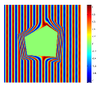
(a) FEM electric field

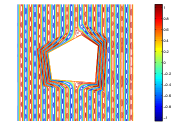
(b) Contour (FEM)

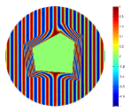
(c) SEM electric field

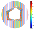
(d) Contour (SEM)

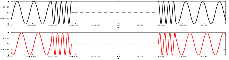
(e) Profiles of the real and imaginary parts of the electric field along $\theta=0$ by SEM

Figure 3.2. A comparison study: SEM versus FEM, where $\theta_{0}=0$ and $k=40.$ In SEM simulation, $40\times 40$-grid is used for each element with a total DOF: $16,000.$ In FEM simulation, a total DOF: $726,933$ is used.

In Figure 3.2, we plot the electric field distribution (real part) for $k=40$ obtained by (i) SEM with $N=40$ in each element and the degree of freedom (DOF): $16,000$, and (ii) FEM with with a total DOF: $726,933$ (in order to obtain reasonable results). Observe that the magnitude of the field obtained from FEM is about $1.05$ (see the colour bar of (a)), which is expected to be $1$ as shown in (c). As a result, the wavefront of the field in the contour appears blurred, while that of the SEM is very accurate. Indeed, the use of exact DtN boundary condition and new CBCs allows us to simulate the ideal cloak very accurately.

We further challenge SEM with higher wavenumber $k=80$ and oblique incident angle $\theta_{0}=\pi/4$ (see Figure 3.3). We depict in (a) the electric field distribution (real part) with cut-off number $M=80$ and $N=80$ in each element with the same geometric setting in Figure 3.2 (c). Again, the highly oscillatory oblique incident wave is perfectly steered by the cloaking layer and completely shielded from the cloaked region. Apart from plotting the electric-field distributions, we also depict the time-averaged Poynting vector (cf. [35]): ${\boldsymbol{S}}={\rm Re}\,\{{\boldsymbol{E}}\times{\boldsymbol{H}}^{*}\}/2,$ which indicates the directional energy flux density. In (b), we depict the associated Poynting vector fields. We find that the waves are again steered smoothly around the polygonal cloaked region without reflecting and scattering.

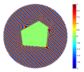
(a) Electric field

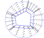
(b) Poynting vector

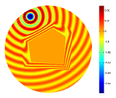
(c) External source

Figure 3.3. SEM with high frequency wave and external source. (a) Real part of the electric field distribution and (b) the related Poynting vector, where $k=80$, $\theta_{0}=\pi/4.$ (c) Real part of the electric field with external source (3.36).

We now add an external source, compactly supported in $\Omega_{+}$ as the wavemaker, and turn off the incident wave. More precisely, we modify (3.24) and (3.26) as

$$\nabla\cdot({\boldsymbol{C}}(\boldsymbol{r})\nabla u^{+}(\boldsymbol{r}))+k^{2}n(\boldsymbol{r})u^{+}(\boldsymbol{r})=f(\boldsymbol{r})\;\;{\rm in}\;\;\Omega_{+};\quad\partial_{r}u^{+}-{\mathscr{T}}_{R}[u^{+}]=0\quad{\rm at}\;\;\Gamma_{\!R}.$$ (3.35)

In practice, we use the Guassian function in Cartesian coordinates:

$$f(\boldsymbol{r})=\alpha\;{\rm exp}\Big{(}{-\frac{(x-\beta)^{2}+(y-\kappa)^{2}}{2\gamma^{2}}}\Big{)},$$ (3.36)

where $\alpha,\beta,\kappa,\gamma$ are tuneable constants. To this end, we take $\alpha=100$, $\beta=-0.41$, $\kappa=0.75$ and $\gamma=0.04,$ so the source at $B_{\!R}$ is nearly zero. The plot of the electric field distributions in Figure 3.3 (c) is computed from SEM with $k=40$, $M=60$ and $N=40$ in each element. The anti-plane waves generated by the source are smoothly bent and the cloak does not produce any scattering. Observe that the waves seamlessly pass through the outer artificial boundary without any reflecting.

3.5. Numerical study of effects of defects, lossy media and dispersive media

We next demonstrate that the proposed SEM provides a reliable tool to study the effect of defects and sensitivity to the variation of the media within the cloaking layer. Interesting investigation (mostly from analytic point of view) has been devoted to the circular and spherical cloaks (see, e.g., [11, 7, 34, 4, 51]), but the tools appear non-trivial to be extended to the polygonal cloaks.

3.5.1. Defects in the cloaking layer

We consider the influence of defects to the perfect polygonal cloak. As illustrated in Figure 3.4 (a)-(b), a rectangular defect with length $a$ and width $b$ is embedded into the cloaking layer. We set $\boldsymbol{C}=\boldsymbol{I}_{2}$ and $n=1$ within the defect, so the traditional transmission condition (2.10) can be imposed at four sides, if the defect is not aligned with the cloaking boundary. In Figure 3.4 (a), we depict the electric field distribution with defect $a=b=0.06$ obtained by the proposed SEM with $k=40$, $\theta_{0}=0$, $M=60$ and $N=40.$ Observe that even with such a small defect, the electric field distribution is apparently disturbed, especially for the forward-scattering region, and the magnitude increases approximately up to $1.5$ (note: it is $1$ for the perfect cloak). Also notice that in the back-scattering region, the waves appear not significantly affected, so the cloaking effects seem still good. In Figure 3.4 (b), we enlarge the defect and set $a=0.24,$ $b=0.06.$ The field in both the back and forward scattering regions is deteriorated more.

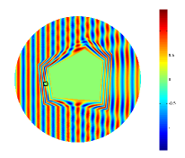
(a) Defect with $a=b=0.06$

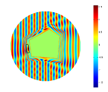
(b) Defect with $a=0.24,\,b=0.06$

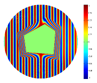
(c) Loss tangent $\tan\delta=0.01$

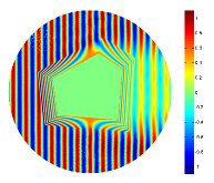
(d) Loss tangent $\tan\delta=0.05$

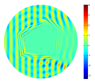
(e) Dispersion with $k=39$

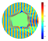
(f) Dispersion with $k=41$

Figure 3.4. The effects of defects, loss and dispersion on the polygonal invisibility cloak. Defects: real part of the electric field distributions with homogeneous defects with sizes (a) $a=b=0.06$ and (b) $a=0.24$, $b=0.06$. Loss: real part of the electric field distributions with loss tangents (c) $\tan\delta=0.01$ and (d) $\tan\delta=0.05$. Dispersion: fix $k_{c}=40$, the real part of the electric field distributions with wave numbers (e) $k=39$ and (f) $k=41$.

3.5.2. Lossy media in the cloaking layer

Similar to the setting in [11, 7] for the circular and spherical cloaks, we replace the media in cloaking layer by a electric-lossy medium (cf. [35]). More precisely, the real electric permittivity $\boldsymbol{\epsilon}$ in (2.2) is replaced by a complex electric permittivity $(1+{\rm i}\tan\delta)\boldsymbol{\epsilon},$ where $\tan\delta$ is a tunable constant termed as loss tangent to quantify the absorptive property of the medium. Note that this replacement only brings about the modification of the two-dimensional Helmholtz equation (2.8) as

$$\nabla\cdot({\boldsymbol{C}}(\boldsymbol{r})\;\nabla u(\boldsymbol{r}))+k^{2}(1+{\rm i}\tan\delta)n(\boldsymbol{r})\,u(\boldsymbol{r})=0.$$

In Figure 3.4, we depict the electric field distributions with loss tangent $\tan\delta=0.01,0.05$ in (c) and (d), respectively, where we take $k=40$, $\theta_{0}=0$, $M=60$ and $N=40$ in each element. Observe that in the first case, the effect of the loss is almost imperceptible. As we enlarge the loss tangent to $0.05$ in (d), the cloaking effect appears good in the backscattering region but is apparently deteriorated in the forward-scattering region, which is inevitable because the lossy medium absorbs the forward-travelling wave power. We point out that similar phenomena were observed for the circular and spherical cloaks in [11, 7].

3.5.3. Drude model and dispersive media in the cloaking layer

Based on the form-invariant coordinate transformation, the polygonal cloak can perfectly conceal arbitrary objects inside the interior polygonal domain. However, as an ideal cloak, the material parameters are dispersive, and perfect invisibility can only be achieved for a single frequency, known as the “cloaking frequency” (cf. [36, 51, 9]). It is of much physical relevance to study the response of an ideal cloak to a non-monochromatic electromagnetic wave passing through such a dispersive cloak. The investigation along this line has been very limited to mostly analytic treatments of circular and spherical cloaks (cf. [4, 51]). We demonstrate that the proposed SEM offers an accurate means to understand some interesting phenomena of a nonmonochromatic wave interacting with a polygonal cloak.

Following the procedure in [34], we start with diagonalizing the symmetric matrices $\boldsymbol{\epsilon}$ and $\boldsymbol{\mu}$ in (2.4)-(2.5), i.e.,

$$\boldsymbol{\epsilon}=\boldsymbol{\mu}={\boldsymbol{P}}{\boldsymbol{\Lambda}}{\boldsymbol{P}}^{t},\quad\boldsymbol{\Lambda}={\rm diag}(\lambda_{1},\lambda_{2},\lambda_{3}),$$ (3.37)

where ${\boldsymbol{P}}=(P_{ij})_{1\leq i,j\leq 3}$ is an orthonormal matrix (with $P_{j3}=P_{3j}=0$ for $j=1,2,$ and $P_{33}=1$), and the eigenvalues are

$$\lambda_{1}=\frac{C_{11}+C_{22}+\sqrt{(C_{11}+C_{22})^{2}-4}}{2},\quad\lambda_{2}=\frac{C_{11}+C_{22}-\sqrt{(C_{11}+C_{22})^{2}-4}}{2},\quad\lambda_{3}=n.$$ (3.38)

From (3.6)-(3.7), we have

$$C_{11}+C_{22}=\frac{r-R_{1}}{r}+\frac{1}{r(r-R_{1})}\Big{(}r^{2}+\Big{(}\frac{dR_{1}}{d\theta}\Big{)}^{2}\Big{)}\geq\frac{r-R_{1}}{r}+\frac{r}{r-R_{1}}\geq 2,$$ (3.39)

which implies $\lambda_{1}>1.$ However, $\lambda_{2}$ and $\lambda_{3}$ are less than $1$ for some $r\in(R_{1},R_{2})$. Based on the principle in [34, 51], we modify $\lambda_{2}$ and $\lambda_{3}$ by using the Drude model (cf. [35]). More precisely, let $\omega_{c}>0$ be the “cloaking frequency”, and define

$$\tilde{\lambda}_{i}:=\tilde{\lambda}_{i}(\boldsymbol{r},\omega)=1-\frac{\omega_{p,i}^{2}}{\omega(\omega+{\rm i}\gamma_{i})},\;\;\;{\rm with}\;\;\;\omega_{p,i}^{2}:=\omega_{c}(\omega_{c}+{\rm i}\gamma_{i})(1-\lambda_{i}),\quad i=2,3,$$ (3.40)

where $\{\gamma_{i}\}_{i=2}^{3}$ are given collision frequencies, and $\{\omega_{p,i}\}_{i=2}^{3}$ are known as the plasma frequencies. For notational convenience, we define

$$\beta_{i}:=\frac{\omega_{c}(\omega_{c}+{\rm i}\gamma_{i})}{\omega(\omega+{\rm i}\gamma_{i})},\;\;\;{\rm so}\;\;\;\tilde{\lambda}_{i}=1+\beta_{i}(\lambda_{i}-1),\quad i=2,3.$$ (3.41)

Denoting $\widetilde{\boldsymbol{\Lambda}}={\rm diag}(\tilde{\lambda}_{1},\tilde{\lambda}_{2},\tilde{\lambda}_{3})$ with $\tilde{\lambda}_{1}=\lambda_{1},$ we then replace the material parameters $\boldsymbol{\epsilon}$ and $\boldsymbol{\mu}$ in (2.2), respectively, by

$$\tilde{\boldsymbol{\epsilon}}=\tilde{\boldsymbol{\mu}}={\boldsymbol{P}}\widetilde{\boldsymbol{\Lambda}}{\boldsymbol{P}}^{t}=\begin{bmatrix}\widetilde{\boldsymbol{C}}&\boldsymbol{0}^{t}\\[2.0pt] \boldsymbol{0}&\tilde{n}\end{bmatrix},$$ (3.42)

where by a direct calculation, we have

$$\widetilde{\boldsymbol{C}}=\begin{bmatrix}\widetilde{C}_{11}&\widetilde{C}_{12}\\[2.0pt] \widetilde{C}_{12}&\widetilde{C}_{22}\end{bmatrix}=\boldsymbol{C}+(1-\beta_{2})(1-\lambda_{2})\begin{bmatrix}P_{12}^{2}&P_{12}P_{22}\\[2.0pt] P_{12}P_{22}&P_{22}^{2}\end{bmatrix},$$ (3.43)

and

$$\tilde{n}=1+\beta_{3}(\lambda_{3}-1)=\tilde{\lambda}_{3}.$$ (3.44)

One verifies readily from (3.42) that

$${\rm det}(\tilde{\boldsymbol{\epsilon}})={\rm det}(\tilde{\boldsymbol{\mu}})=\tilde{\lambda}_{1}\tilde{\lambda}_{2}\tilde{\lambda}_{3}=\lambda_{1}\tilde{\lambda}_{2}\,\tilde{n}={\rm det}(\widetilde{\boldsymbol{C}})\,\tilde{n}.$$ (3.45)

Thus, using the fact $\lambda_{1}\lambda_{2}=1$ (cf. (3.38)), we obtain from (3.41) and (3.45) that

$${\rm det}(\widetilde{\boldsymbol{C}})=\lambda_{1}\tilde{\lambda}_{2}=\lambda_{1}(\beta_{2}\lambda_{2}+1-\beta_{2})=\beta_{2}+(1-\beta_{2})\lambda_{1}.$$ (3.46)

Accordingly, we find that the counterpart of (2.6) becomes

$$\tilde{\boldsymbol{\mu}}^{-1}=\tilde{\boldsymbol{\epsilon}}^{-1}=\begin{bmatrix}\widehat{C}_{22}&-\widehat{C}_{12}&0\\[1.0pt] -\widehat{C}_{12}&\widehat{C}_{11}&0\\[1.0pt] 0&0&\tilde{n}^{-1}\end{bmatrix},\;\;\;{\rm where}\;\;\;\widehat{C}_{ij}=\frac{\widetilde{C}_{ij}}{\beta_{2}+(1-\beta_{2})\lambda_{1}},$$ (3.47)

for $i,j=1,2.$ Using (2.7) with $\widehat{C}_{ij}$ and $\tilde{n}$ in place of $C_{ij}$ and $n$, we obtain the new model defined in the cloaking layer:

$$\nabla\cdot\big{(}\widehat{\boldsymbol{C}}(\boldsymbol{r},\omega)\;\nabla u(\boldsymbol{r})\big{)}+k^{2}\,\tilde{n}(\boldsymbol{r},\omega)\,u(\boldsymbol{r})=0,$$ (3.48)

where $\widehat{\boldsymbol{C}}=(\widehat{C}_{ij})_{1\leq i,j\leq 2},$ and $k=\omega\sqrt{\epsilon_{0}\mu_{0}}$ as before.

Remark 3.4.

Observe from (3.41) that if $\omega=\omega_{c},$ then $\beta_{i}=1$ and $\lambda_{i}=\tilde{\lambda}_{i}$ for $i=1,2.$ Thus, in this case, (3.48) reduces to (2.8) and $\widehat{\boldsymbol{C}}(\boldsymbol{r},\omega_{c})$ is singular at the cloaking boundary $r=R_{1}$. However, if $\omega\not=\omega_{c}$ (so $\beta_{2}\not=1$), then $\widehat{\boldsymbol{C}}(\boldsymbol{r},\omega)$ becomes regular at $r=R_{1}.$ Indeed, by (3.47),

$$\widehat{C}_{ij}=\frac{(r-R_{1})\widetilde{C}_{ij}}{\beta_{2}(r-R_{1})+(1-\beta_{2})(r-R_{1})\lambda_{1}}.$$

In fact, one can verify that if $\beta_{2}\not=1,$

$$\lim_{r\to R_{1}}(r-R_{1})\big{\{}\boldsymbol{C},\lambda_{1},\lambda_{2}\big{\}}\;\;\text{all exist}.$$

Thus, we can claim from (3.43) and the above that $\widehat{\boldsymbol{C}}(\boldsymbol{r},\omega)$ is well-defined at $r=R_{1}.$ In view of this, the CBCs can not be applied. Here, we follow [4, 51] and impose a PMC shell instead. ∎

In the computation, we take $\omega_{c}=k_{c}/\sqrt{\epsilon_{0}\mu_{0}}$ with $k_{c}=40,$ and $\gamma_{i}/\sqrt{\epsilon_{0}\mu_{0}}=0.0001$ for $i=2,3$. In Figure 3.4 (e)-(f), we plot the electric field distributions with $k=39$ and $k=41$ illuminated by plane wave in (3.34) with incident angle $\theta_{0}=0$ and the cut-off number $M=60$ and $N=45$ in each element. In contrast with Figure 3.2 (c) (where perfect cloaking effect can be obtained for $k_{c}=40$), we observe from Figure 3.4 that the electric field distributions are affected and distorted in both cases (i.e., $k=k_{c}\pm 1$), in particular, more severely when $k<k_{c}.$ Indeed, similar to the phenomena observed in [51, 4] for circular and spherical cloaks, the incident wave with frequency slightly deviated below $k_{c}$, the field after the wave passes the cloak is dissipated and a large shadow appears in the forward scattering region. While for the incident wave with frequency slightly deviated above $k_{c}$, the field in most part of the cloaking layer does not change much, except for the part close to the cloaking boundary $r=R_{1}$, and the field behind the cloak is reinforced. This can be regarded as the frequency shift effect as in [51].

4. Accurate simulation of electromagnetic concentrators and rotators

In this section, we further apply the efficient spectral-element solver to accurately simulate the electromagnetic concentrators and rotators.

4.1. Polygonal concentrators

The electromagnetic concentrator aims at intensifying electromagnetic waves in a certain region, which play an important role in the harnessing of light in solar cells or similar devices, where high field intensities are needed.

Here, we are interested in the polygonal concentrator with a configuration similar to the polygonal cloak illustrated in Figure 4.1 (b), where EM waves are expected to be concentrated in the interior convex polygonal region $\Omega_{-}^{p}$. It is accomplished by a coordinate transformation that maps the “polygonal annulus” in Figure 4.1 (a) to the “polygonal annulus” in Figure 4.1 (b), where the interior portion of the latter has larger area. More precisely, the polygonal concentrator is mapped from the same structure in Figure 4.1 (b) but with a different ratio (see Figure 4.1 (a)):

$$\breve{\rho}=\frac{OA_{o}}{OA}=\frac{OB_{o}}{OB}=\cdots,\quad 0<\rho<\breve{\rho}<1,$$ (4.1)

where $\rho$ is defined in (3.3). Then the ratio $\rho/\breve{\rho}$ is known as the rate of concentration. For notational convenience, we define

$$\varrho:=1-\dfrac{1-\rho}{1-\breve{\rho}}.$$ (4.2)

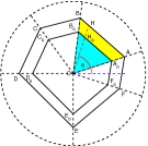
(a) $(\breve{x},\breve{y})$-domain

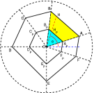
(b) $(x,y)$-domain

(c) Circular rotator

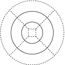
(d) Partition of $B_{R}$

Figure 4.1. Schematic geometry of a polygonal concentrator and a circular rotator. (a) The polygonal domain in the original coordinates $(\breve{x},\breve{y}).$ (b) Through the coordinate transformation (4.3), the polygonal domain $\Omega_{-}^{o}=A_{o}B_{o}\cdots F_{o}$ is compressed into the polygonal domain $\Omega_{-}^{p}$ that forms the concentration region. Consequently, the original polygonal annulus domain $\Omega_{-}\setminus\bar{\Omega}_{-}^{o}$ in (a) is expanded into the polygonal annulus $\Omega_{-}^{a}$. (c) Through the coordinate transformation (4.13), points in the circular annulus $a<r<b$ are rotated with a fixed angle $\theta_{1}$. (d) The computational mesh for the circular rotator.

The corresponding coordinate transformation takes the form (see, e.g., [20]):

• In $\Omega_{-}$,

  $$\begin{cases}r=\dfrac{\rho}{\breve{\rho}}\,\breve{r},\quad&\breve{r}\in[0,\breve{R}_{1}],\;\;r\in[0,R_{1}],\\[8.0pt] r=(1-\varrho)\,\breve{r}+\varrho\,R_{2},\quad&\breve{r}\in[\breve{R}_{1},R_{2}],\;\;r\in[R_{1},R_{2}],\end{cases}$$ (4.3)

  and $\theta=\breve{\theta}\in[0,2\pi);$

• In $\Omega_{+}=B_{R}\setminus\bar{\Omega}_{-}$, the transformation is identity: $r=\breve{r},\;\theta=\breve{\theta}.$

Here, $R_{i},\;i=1,2,$ are the same as in (3.5) and $\breve{R}_{1}=\breve{\rho}/\rho R_{1}.$ Using (2.5), we can derive the coefficients $\boldsymbol{C}$ and $n$ as follows (see Appendix A):

• In $\Omega_{-}^{\rm p}$,

  $${\boldsymbol{C}}={\boldsymbol{I}}_{2},\quad n={\breve{\rho}^{2}}/{\rho^{2}}\,.$$ (4.4)

• In $\Omega_{-}^{\rm a}$,

  $$C_{11} =\frac{r-\varrho R_{2}}{r}\,\frac{x^{2}}{r^{2}}+\frac{\varrho}{r-\varrho R_{2}}\bigg{(}\frac{\varrho}{r}\frac{{\rm d}R_{2}}{{\rm d}\theta}\frac{x^{2}}{r^{2}}-\frac{2xy}{r^{2}}\bigg{)}\frac{{\rm d}R_{2}}{{\rm d}\theta}+\frac{r}{r-\varrho R_{2}}\,\frac{y^{2}}{r^{2}},$$ (4.5)

  $$C_{22} =\frac{r-\varrho R_{2}}{r}\,\frac{y^{2}}{r^{2}}+\frac{\varrho}{r-\varrho R_{2}}\bigg{(}\frac{\varrho}{r}\frac{{\rm d}R_{2}}{{\rm d}\theta}\frac{y^{2}}{r^{2}}+\frac{2xy}{r^{2}}\bigg{)}\frac{{\rm d}R_{2}}{{\rm d}\theta}+\frac{r}{r-\varrho R_{2}}\,\frac{x^{2}}{r^{2}},$$ (4.6)

  $$C_{12} =\bigg{(}\frac{r-\varrho R_{2}}{r}-\frac{r}{r-\varrho R_{2}}\bigg{)}\,\frac{xy}{r^{2}}+\frac{\varrho}{r-\varrho R_{2}}\bigg{(}\frac{x^{2}}{r^{2}}+\frac{\varrho}{r}\frac{{\rm d}R_{2}}{{\rm d}\theta}\frac{xy}{r^{2}}-\frac{y^{2}}{r^{2}}\bigg{)}\frac{{\rm d}R_{2}}{{\rm d}\theta},$$ (4.7)

  and

  $$n=\frac{r-\varrho R_{2}}{r(1-\varrho)^{2}}\,.$$ (4.8)

• In $\Omega_{+}$, we have $\boldsymbol{C}=\boldsymbol{I}_{2}$ and $n=1.$

In summary, the governing equation for the polygonal concentrator reads

$$\nabla\cdot({\boldsymbol{C}}(\boldsymbol{r})\,\nabla u(\boldsymbol{r}))+k^{2}n(\boldsymbol{r})u(\boldsymbol{r})=0\quad{\rm in}\;\;B_{R},$$ (4.9)

$$\llbracket u\rrbracket=\llbracket\boldsymbol{C}\,\nabla u\rrbracket=0\quad{\rm at}\;\;\Gamma^{p}\cup\Gamma^{a},$$ (4.10)

$$\partial_{r}u-{\mathscr{T}}_{R}[u]=h\quad{\rm at}\;\;\partial B_{R}.$$ (4.11)

Note that in the interior polygon, (4.9) becomes the Helmholtz equation:

$$\Delta u+\frac{\breve{\rho}^{2}}{\rho^{2}}k^{2}u=0\quad{\rm in}\;\;\Omega_{-}^{p},$$ (4.12)

where the ratio ${\breve{\rho}^{2}}/{\rho^{2}}>1$ is a constant. Therefore, the coordinate transformation enlarges the wavenumber $k$ that produces the effect of concentration.

We can implement the spectral-element solver based on the partition of the computational domain as with the previous application. However, different from the previous case, the interior region is part of the computational domain, where a normal transmission condition is imposed along its boundary (see (4.10)). Below, we provide some numerical results with the setting: a square concentrator centred at the origin with length of each side $1.2$ and the parameters: $\rho=1/3,\;\breve{\rho}=2/3$ in (3.3) and (4.1) and $R=1.0.$ We set the cut-off number $M=60$ in the DtN operator. In Figure 4.2, we depict the electric field distributions and the associated time averaged Poynting vectors illuminated with different incident angles ((a)-(b): $\theta_{0}=0$ and (c)-(d): $\theta_{0}=\pi/4$) with $k=40$ and the grid $N=50$ in each element. It can be seen that the electric field and energy flux are smoothly concentrated into the inner concentration region $\Omega_{-}^{p}$, and the field outside is not affected regardless of the incident angle on the concentrator.

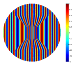
(a) Electric field with $\theta_{0}=0$

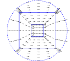
(b) Poynting vector

(c) Electric field with $\theta_{0}=\pi/4$

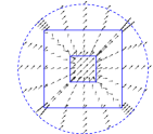
(d) Poynting vector

Figure 4.2. The real part of the electric field distributions and associated Poynting vectors for square concentrators with (a)-(b): $\theta_{0}=0$ and (c)-(d): $\theta_{0}=\pi/4$, respectively.

4.2. Circular rotators

In contrast with the invisibility cloak and concentrator, the electromagnetic rotator is based upon a coordinate transformation of the angular variable rather than the radial variable in (3.1).

As illustrated in Figure 4.1 (c), the domain $\Omega_{-}$ is a disk of radius $r=b,$ which encloses a concentric disk of radius $r=a<b.$ The waves are expected to rotate with a fixed angle $\theta_{1}$ in the interior disk. This can be realised by the coordinate transformation (cf. [8]):

$$\begin{cases}r=\breve{r},\;\;\;\theta=\breve{\theta}+\theta_{1},\quad&0<\breve{r}<a,\;\;\breve{\theta},\,\theta\in[0,2\pi),\\[8.0pt] r=\breve{r},\;\;\;\theta=\breve{\theta}+\dfrac{s(b)-s(\breve{r})}{{s}(b)-s(a)}\theta_{1},\quad&a<\breve{r}<b,\;\;\breve{\theta},\,\theta\in[0,2\pi),\end{cases}$$ (4.13)

where $s$ is any smooth function such that $s(b)\not=s(a).$ As before, the transformation is identity exterior to $\Omega_{-}.$

Define

$$\kappa=\dfrac{s(r)^{\prime}}{{s}(b)-s(a)}\,\theta_{1}.$$ (4.14)

Working out the material parameters as before (see Appendix A), we have

$${\boldsymbol{C}}=\frac{1}{r^{2}}\begin{bmatrix}r^{2}+2\kappa xy+\kappa^{2}y^{2}&-\kappa x^{2}-\kappa^{2}xy+\kappa y^{2}\;\\[3.0pt] -\kappa x^{2}-\kappa^{2}xy+\kappa y^{2}&r^{2}-2\kappa xy+\kappa^{2}x^{2}\;\end{bmatrix},\;\;\;n=1\quad{\rm for}\;\;a<r<b,$$ (4.15)

and

$${\boldsymbol{C}}={\boldsymbol{I}}_{2},\quad n=1\quad{\rm for}\;\;0<r<a,\;\;b<r<R.$$ (4.16)

In Figure 4.1 (d), we illustrate a partition of the computational domain $B_{R}.$ Together with the standard transmission conditions in (2.12), we can implement the spectral element scheme as the previous cases with a similar partition of the computational domain (see Figure 4.1 (d)). In the computation, we set $a=0.3,\;b=0.7$ and $s(r)=r$ in (4.13) and choose $R=1.0$, $M=60$ and $N=40$ in each element. In Figure 4.3, we fix $k=40$, and plot the electric field distribution (real part) and the corresponding time averaged Poynting vector with the same incident angle $\theta_{0}=0$ and different rotation angles ((a)-(b): $\theta_{1}=\pi/4$, (c)-(d): $\theta_{1}=3\pi/4$). We find that the electric field distribution rotates its direction by $\pi/4$ in Figure 4.3 (a) and the power flux (b) flows with the same direction in the closed region $r<a$. It can be observed in Figure 4.3 (c)-(d) that even for a very sharp rotation angle $\theta_{1}=3\pi/4$, the field rotates exactly by $3\pi/4$ angle without introducing any scattering wave outside.

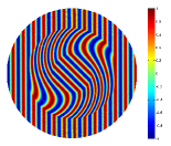
(a) Electric field with $\theta_{1}=\pi/4$

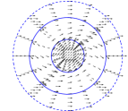
(b) Poynting vector

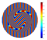
(c) Electric field with $\theta_{1}=3\pi/4$

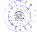
(d) Poynting vector

Figure 4.3. The real part of the electric field distributions and associated Poynting vectors for circular rotators with (a)-(b): $\theta_{1}=\pi/4$ and (c)-(d): $\theta_{1}=3\pi/4$, respectively.

Concluding remarks

In this paper, we presented an accurate and efficient spectral-element solver for time-harmonic Helmholtz equations in general inhomogeneous and anisotropic media. We focused on several applications arisen from transformation electromagnetics which included the polygonal invisibility cloaks and concentrators, and circular rotators. We introduced new ideas of how to seamlessly integrate local elements and global DtN boundary condition. This can shed light on the three-dimensional simulation where the DtN BC involves spherical harmonic expansions. We proposed new cloaking boundary conditions for accurate simulation of perfect polygonal invisibility cloaks. The proposed method also provided a reliable alternative to the analytic tools to study the interesting phenomena when defects and other media were embedded or placed in a perfect cloak.

Appendix A Derivation of material parameters for polygonal cylindrical cloaks, concentrators and circular rotators

As illustrated by (3.1) in Section 3, the transformation is given from polar coordinates $(\breve{r},\breve{\theta})$ (of the original Cartesian coordinates $(\breve{x},\breve{y})$) to polar coordinates $(r,\theta)$ (of the physical Cartesian coordinates $(x,y)$), so by the chain rule, the Jacobian matrix $\boldsymbol{J}_{\!{\rm cn}}$ can be computed by

$$\boldsymbol{J}_{\!{\rm cn}}=\begin{bmatrix}\partial_{\breve{x}}x&\partial_{\breve{y}}x\\[1.0pt] \partial_{\breve{x}}y&\partial_{\breve{y}}y\\[1.0pt] \end{bmatrix}=\begin{bmatrix}\partial_{r}x&\partial_{\theta}x\\[1.0pt] \partial_{r}y&\partial_{\theta}y\\[1.0pt] \end{bmatrix}\begin{bmatrix}\partial_{\breve{r}}r&\partial_{\breve{\theta}}r\\[1.0pt] \partial_{\breve{r}}\theta&\partial_{\breve{\theta}}\theta\\[1.0pt] \end{bmatrix}\begin{bmatrix}\partial_{\breve{x}}\breve{r}&\partial_{\breve{y}}\breve{r}\\[0.5pt] \partial_{\breve{x}}\breve{\theta}&\partial_{\breve{y}}\breve{\theta}\\[0.5pt] \end{bmatrix}.$$ (A.1)

It is clear that

$$\begin{bmatrix}\partial_{r}x&\partial_{\theta}x\\[1.0pt] \partial_{r}y&\partial_{\theta}y\\[1.0pt] \end{bmatrix}=\begin{bmatrix}\cos\theta&-r\sin\theta\\[1.0pt] \sin\theta&r\cos\theta\\[1.0pt] \end{bmatrix},\quad{\rm det}\bigg{(}\begin{bmatrix}\partial_{r}x&\partial_{\theta}x\\[1.0pt] \partial_{r}y&\partial_{\theta}y\\[1.0pt] \end{bmatrix}\bigg{)}=r,$$ (A.2)

and

$$\begin{bmatrix}\partial_{\breve{x}}\breve{r}&\partial_{\breve{y}}\breve{r}\\[0.5pt] \partial_{\breve{x}}\breve{\theta}&\partial_{\breve{y}}\breve{\theta}\\[0.5pt] \end{bmatrix}=\begin{bmatrix}\cos\breve{\theta}&\sin\breve{\theta}\\[0.1pt] -\sin\breve{\theta}/\breve{r}&\cos\breve{\theta}/\breve{r}\\[0.1pt] \end{bmatrix},\quad{\rm det}\bigg{(}\begin{bmatrix}\partial_{\breve{x}}\breve{r}&\partial_{\breve{y}}\breve{r}\\[0.5pt] \partial_{\breve{x}}\breve{\theta}&\partial_{\breve{y}}\breve{\theta}\\[0.5pt] \end{bmatrix}\bigg{)}=\frac{1}{\breve{r}}.$$ (A.3)

Denote

$${\boldsymbol{\tilde{J}}}:=\begin{bmatrix}\partial_{\breve{r}}r&\partial_{\breve{\theta}}r\\[1.0pt] \partial_{\breve{r}}\theta&\partial_{\breve{\theta}}\theta\\[1.0pt] \end{bmatrix},$$ (A.4)

which is determined by specific coordinate transformations. With a direct calculation, we derive from (2.5) the material parameters $\boldsymbol{C}$ and $n$ for the general transformation in (3.1):

$$C_{11} =\frac{\breve{r}}{r^{3}{\rm det}(\boldsymbol{\tilde{J}})}\Big{(}\big{(}x\partial_{\breve{r}}r-ry\partial_{\breve{r}}\theta\big{)}^{2}+\frac{1}{\breve{r}^{2}}\big{(}x\partial_{\breve{r}}\theta-ry\partial_{\breve{\theta}}\theta\big{)}^{2}\Big{)}\,,$$ (A.5)

$$C_{22} =\frac{\breve{r}}{r^{3}{\rm det}(\boldsymbol{\tilde{J}})}\Big{(}\big{(}y\partial_{\breve{r}}r+rx\partial_{\breve{r}}\theta\big{)}^{2}+\frac{1}{\breve{r}^{2}}\big{(}y\partial_{\breve{r}}r+rx\partial_{\breve{\theta}}\theta\big{)}^{2}\Big{)}\,,$$ (A.6)

$$C_{12} =\frac{\breve{r}}{r^{3}{\rm det}(\boldsymbol{\tilde{J}})}\Big{(}xy\Big{(}\partial^{2}_{\breve{r}}r+\frac{1}{\breve{r}^{2}}\partial^{2}_{\breve{\theta}}r-r^{2}\partial^{2}_{\breve{r}}\theta-\frac{r^{2}}{\breve{r}^{2}}\partial^{2}_{\breve{\theta}}\theta\Big{)}+\frac{(x^{2}-y^{2})r}{\breve{r}^{2}}\big{(}\breve{r}^{2}\partial_{\breve{r}}r\partial_{\breve{r}}\theta+\partial_{\breve{\theta}}r\partial_{\breve{\theta}}\theta\big{)}\Big{)},$$ (A.7)

and

$$n=\frac{1}{{\rm det}(\boldsymbol{J}_{\!{\rm cn}})}=\frac{\breve{r}}{r{\rm det}(\boldsymbol{\tilde{J}})}\,.$$ (A.8)

For the polygonal cylindrical cloak, we derive from (3.2) that in $\Omega_{-}^{a}$,

$$\breve{r}=\dfrac{1}{1-\rho}(r-\,R_{1}),\quad\breve{\theta}=\theta,$$ (A.9)

which leads to

$$\boldsymbol{\tilde{J}}=\begin{bmatrix}1-\rho&\partial_{\theta}R_{1}\\[1.0pt] 0&1\\[1.0pt] \end{bmatrix},\quad\rm{det}(\boldsymbol{\tilde{J}})=1-\rho.$$ (A.10)

Recall that $\partial_{\theta}R_{1}$ can be worked out by (3.5). Thus, the material parameters $\boldsymbol{C}$ and $n$ in (3.6)-(3.9) can be obtained by substituting (A.9)-(A.10) into (A.5)-(A.8).

Similarly, for the polygonal cylindrical concentrator, we obtain from the transformation (4.3) that in $\Omega_{-}^{\rm a}$,

$$\breve{r}=\frac{1}{1-\varrho}(r-\varrho R_{2}),\quad\breve{\theta}=\theta,$$ (A.11)

and

$$\boldsymbol{\tilde{J}}=\begin{bmatrix}1-\varrho&\varrho\partial_{\theta}R_{2}\\[1.0pt] 0&1\\[1.0pt] \end{bmatrix},\quad\rm{det}(\boldsymbol{\tilde{J}})=1-\varrho\,.$$ (A.12)

Inserting (A.11) and (A.12) into (A.5)-(A.8), we obtain $\boldsymbol{C}$ and $n$ in (4.5)-(4.8).

For the circular rotators, we have from (4.13) that

$$\breve{r}=r,\;\;\;\breve{\theta}=\theta-\dfrac{s(b)-s(r)}{{s}(b)-s(a)}\theta_{1},$$ (A.13)

and

$$\begin{bmatrix}\partial_{\breve{r}}r&\partial_{\breve{\theta}}r\\[1.0pt] \partial_{\breve{r}}\theta&\partial_{\breve{\theta}}\theta\\[1.0pt] \end{bmatrix}=\begin{bmatrix}1&0\\[1.0pt] -\kappa&1\\[1.0pt] \end{bmatrix},$$ (A.14)

where $\kappa$ is defined in (4.14). Then we can compute the material parameters (4.14) in a similar fashion.

References

- [1] M. Abramowitz and I.A. Stegun, editors. Handbook of Mathematical Functions with Formulas, Graphs, and Mathematical Tables. A Wiley-Interscience Publication. John Wiley & Sons Inc., New York, 1984. Reprint of the 1972 edition, Selected Government Publications.
- [2] R.A. Adams and J.J. Fournier. Sobolev Spaces, volume 140. Academic press, 2003.
- [3] G.B. Arfken and H.J. Weber. Mathematical Methods for Physicists. Harcourt/Academic press, 2001.
- [4] C. Argyropoulos, E. Kallos, and Y. Hao. Dispersive cylindrical cloaks under nonmonochromatic illumination. Phys. Rev. E., 81(1):016611, 2010.
- [5] J.P. Berenger. A perfectly matched layer for the absorption of electromagnetic waves. J. Comput. Phys., 114(2):185–200, 1994.
- [6] C. Canuto, M.Y. Hussaini, A. Quarteroni, and T.A. Zang. Spectral Methods: Evolution to Complex Geometries and Applications to Fluid Dynamics. Springer, 2007.
- [7] H.S. Chen, B.I. Wu, B.L. Zhang, and J.A. Kong. Electromagnetic wave interactions with a metamaterial cloak. Phys. Rev. Lett., 99:063903, 2007.
- [8] H.Y. Chen and C.T. Chan. Transformation media that rotate electromagnetic fields. Appl. Phys. Lett., 90(24):241105, 2007.
- [9] H.Y. Chen, Z.X. Liang, P.J. Yao, X.Y. Jiang, H.R. Ma, and C.T. Chan. Extending the bandwidth of electromagnetic cloaks. Phys. Rev. B., 76(24):241104, 2007.
- [10] H.Y. Chen, X.D. Luo, H.R. Ma, and C.T. Chan. The anti-cloak. Opt. Express, 16(19):14603–14608, 2008.
- [11] S. Cummer, B. Popa, D. Schurig, D. Smith, and J.B. Pendry. Full-wave simulations of electromagnetic cloaking structures. Phys. Rev. E., 74(3):036621, 2006.
- [12] M.O. Deville, P.F. Fischer, and E.H. Mund. High-Order Methods for Incompressible Fluid Flow, volume 9. Cambridge University Press, 2002.
- [13] B. Engquist and A. Majda. Absorbing boundary conditions for the numerical simulation of waves. Math. Comp., 31(139):629–651, 1977.
- [14] A. Fournier. Exact calculation of fourier series in nonconforming spectral-element methods. J. Comput. Phys., 215:1–5, 2006.
- [15] W.J. Gordon and C.A. Hall. Transfinite element methods: blending-function interpolation over arbitrary curved element domains. Numer. Math., 21(2):109–129, 1973.
- [16] A. Greenleaf, Y. Kurylev, M. Lassas, and G. Uhlmann. Cloaking devices, electromagnetic wormholes, and transformation optics. SIAM Rev., 51(1):3–33, 2009.
- [17] M.J. Grote and J.B. Keller. On non-reflecting boundary conditions. J. Comput. Phys., 122:231–243, 1995.
- [18] T. Hagstrom. Radiation boundary conditions for the numerical simulation of waves. Acta numer., 8:47–106, 1999.
- [19] Y. He, M. Min, and D.P. Nicholls. A spectral element method with transparent boundary condition for periodic layered media scattering.
- [20] W.X. Jiang, T.J. Cui, Q. Cheng, J.Y. Chin, X.M. Yang, R.P. Liu, and D.R. Smith. Design of arbitrarily shaped concentrators based on conformally optical transformation of nonuniform rational b-spline surfaces. Appl. Phys. Lett., 92(26):264101, 2008.
- [21] W.X. Jiang, T.J. Cui, G.X. Yu, X.Q. Lin, Q. Cheng, and J.Y. Chin. Arbitrarily elliptical–cylindrical invisible cloaking. J. Phys. D: Appl. Phys., 41(8):085504, 2008.
- [22] J.M. Jin, J.L. Volakis, and J.D. Collins. A finite element-boundary integral method for scattering and radiation by two-and three-dimensional structures. IEEE Antennas. Propag. Mag., 33(3):22–32, 1991.
- [23] G. Karniadakis and S. Sherwin. Spectral/hp Element Methods for Computational Fluid Dynamics. Oxford University Press, 2005.
- [24] D.H. Kwon and D.H. Werner. Two-dimensional eccentric elliptic electromagnetic cloaks. Appl. Phys. Lett., 92(1):013505, 2008.
- [25] M. Lassas and T. Zhou. Singular partial differential operators and pseudo-differential boundary conditions in invisibility cloaking. In Fourier Analysis, Trends in Mathematics, pages 263–284, 2014. Springer, Switzerland.
- [26] M. Lassas and T. Zhou. Two dimensional invisibility cloaking for Helmholtz equation and non-local boundary conditions. Math. Res. Lett., 18(3):473–488, 2011.
- [27] U. Leonhardt. Optical conformal mapping. Science, 312(5781):1777–1780, 2006.
- [28] J.C. Li and Y.Q. Huang. Mathematical simulation of cloaking metamaterial structures. Adv. Appl. Math. Mech, 4:93–101, 2012.
- [29] J.C. Li, Y.Q. Huang, and W. Yang. Developing a time-domain finite-element method for modeling of electromagnetic cylindrical cloaks. J. Comput. Phys., 231(7):2880–2891, 2012.
- [30] Y. Lin, J.H. Lee, J.G. Liu, M. Chai, J. A. Mix, and Q.H. Liu. A hybrid SIM-SEM method for 3-D electromagnetic scattering problems. IEEE Trans. Antennas. Propag., 57(11):3655–3663, 2009.
- [31] H. Ma, S.B. Qu, Z. Xu, J.Q. Zhang, B.W. Chen, and J.F. Wang. Material parameter equation for elliptical cylindrical cloaks. Phys. Rev. A., 77(1):013825, 2008.
- [32] P. Monk. Finite Element Methods for Maxwell’s Equations. Numerical Mathematics and Scientific Computation. Oxford University Press, New York, 2003.
- [33] J.C. Nédélec. Acoustic and Electromagnetic Equations, volume 144 of Applied Mathematical Sciences. Springer-Verlag, New York, 2001. Integral representations for harmonic problems.
- [34] N. Okada and J.B. Cole. FDTD modeling of a cloak with a nondiagonal permittivity tensor. ISRN. Opt., 2012:063903, 2012.
- [35] S.J. Orfanidis. Electromagnetic Waves and Antennas. Rutgers University, 2002.
- [36] J.B. Pendry, D. Schurig, and D.R. Smith. Controlling electromagnetic fields. Science, 312(5781):1780–1782, 2006.
- [37] E.J. Post. Formal Structure of Electromagnetics: General Covariance and Electromagnetics. Courier Corporation, 1997.
- [38] M. Rahm, D.A. Roberts, J.B. Pendry, and D.R. Smith. Transformation-optical design of adaptive beam bends and beam expanders. Opt. Express, 16(15):11555–11567, 2008.
- [39] M. Rahm, D. Schurig, D.A. Roberts, S.A. Cummer, D.R. Smith, and J.B. Pendry. Design of electromagnetic cloaks and concentrators using form-invariant coordinate transformations of maxwell s equations. Phot. Nano. Fund. Appl., 6(1):87–95, 2008.
- [40] C. Ronchi, R. Lacono, and P.S. Paolucci. The cubed sphere : a new method for the solution of partial differential equations in spherical geometry. J. Comput. Phys., 124(1):93–114, 1996.
- [41] Z. Ruan, M. Yan, C.W. Neff, and M. Qiu. Ideal cylindrical cloak: perfect but sensitive to tiny perturbations. Phys. Rev. Lett., 99(11):113903, 2007.
- [42] J. Shen, T. Tang, and L.L. Wang. Spectral Methods: Algorithms, Analysis and Applications, volume 41 of Springer Series in Computational Mathematics. Springer-Verlag, Berlin, Heidelberg, 2011.
- [43] R. Weder. The boundary conditions for point transformed electromagnetic invisibility cloaks. J. Phys. A: Math. Theor., 41(41):415401, 2008.
- [44] D.H. Werner and D.H. Kwon. Transformation Electromagnetics and Metamaterials. Springer, 2013.
- [45] Q. Wu, K. Zhang, F.Y. Meng, and L.W. Li. Material parameters characterization for arbitrary -sided regular polygonal invisible cloak. J. Phys. D: Appl. Phys., 42(3):035408, 2009.
- [46] M. Yan, W. Yan, and M. Qiu. Cylindrical superlens by a coordinate transformation. Phys. Rev. B., 78(12):125113, 2008.
- [47] T. Yang, H.Y. Chen, X.D. Luo, and H.R. Ma. Superscatterer: enhancement of scattering with complementary media. Opt. Express, 16(22):18545–18550, 2008.
- [48] Z.G. Yang and L.L. Wang. Accurate simulation of ideal circular and elliptic cylindrical invisibility cloaks. Commun. Comput. Phys., 17(03):822–849, 2015.
- [49] B.L. Zhang. Electrodynamics of transformation-based invisibility cloaking. Light: Science & Applications, 1(10):e32, 2012.
- [50] B.L. Zhang, H.S. Chen, B.I. Wu, Y. Luo, L. Ran, and J.A. Kong. Response of a cylindrical invisibility cloak to electromagnetic waves. Phys. Rev. B., 76(12):121101, 2007.
- [51] B.L. Zhang, B.I. Wu, H.S. Chen, and J.A. Kong. Rainbow and blueshift effect of a dispersive spherical invisibility cloak impinged on by a nonmonochromatic plane wave. Phys. Rev. Lett., 101(6):063902, 2008.
- [52] J. Zhang, L.L. Wang, and Z.J. Rong. A prolate-element method for nonlinear PDEs on the sphere. J. Sci. Comput., 47(1):73–92, 2011.
- [53] J.J. Zhang, Y. Luo, H.S. Chen, and B.I. Wu. Cloak of arbitrary shape. J. Opt. Soc. Am. B., 25(11):1776–1779, 2008.
- [54] Y. Zhao, C. Argyropoulos, and Y. Hao. Full-wave finite-difference time-domain simulation of electromagnetic cloaking structures. Opt. Express, 16(9):6717–6730, 2008.