Multi-level segment analysis: definition and application in turbulent systems

Abstract

For many complex systems the interaction of different scales is among the most interesting and challenging features. It seems not very successful to extract the physical properties in different scale regimes by the existing approaches, such as structure-function and Fourier spectrum method. Fundamentally these methods have their respective limitations, for instance scale mixing, i.e. the so-called infrared and ultraviolet effects. To make improvement in this regard, a new method, multi-level segment analysis (MSA) based on the local extrema statistics, has been developed. Benchmark (fractional Brownian motion) verifications and the important case tests (Lagrangian and two-dimensional turbulence) show that MSA can successfully reveal different scaling regimes, which has been remaining quite controversial in turbulence research. In general the MSA method proposed here can be applied to different dynamic systems in which the concepts of multiscaling and multifractal are relevant.

Keywords: intermittency, multifractal, two-dimensional turbulence, Lagrangian turbulence

1 Introduction

Multiscale is one of the most important features commonly existing in complex systems, where a large range of spatial/temporal scales coexist and interact with each other. Typically such interaction generates scaling relations in the respective scale ranges. To understand the multiscale statistical behavior has been remaining as the research focus in various areas, such as fluid turbulence (Frisch, 1995), financial market analysis (Mantegna and Stanley, 1996; Schmitt et al., 1999; Li and Huang, 2014), environmental science (Schmitt et al., 1998) and population dynamics (Seuront et al., 1999), to list a few. Among a number of existing analysis approaches for such problems, the standard and most cited one is structure-function (SF), which is first introduced by Kolmogorov in his famous homogeneous and isotropic turbulence theory in 1941 (Kolmogorov, 1941; Frisch, 1995). However, the average operation in SF mixes regions with different correlations (Wang and Peters, 2006, 2008). Mathematically, SF acts as a filter with a weight function of $W(k,\ell)=1-\cos(2\pi k\ell)$, in which $k$ is the wavenumber and $\ell$ is the separation scale (Davidson and Pearson, 2005; Huang et al., 2010). It thus makes the statistics at different scale $\ell$ strongly mixed, resulting in the so-called infrared and ultraviolet effects, respectively for large-scale and small-scale contamination (Huang et al., 2013). The situation will be more serious when an energetic structure presents, e.g., annual cycle in collected geoscience data (Huang et al., 2009), large-scale circulations in Rayleigh-Bénard convection, vortex trapping events in Lagrangian turbulence (Huang et al., 2013; Wang, 2014).

Fourier analysis in the frequency domain has the similar deficiency as SF, i.e. any local event will propagate the influence over the entire analyzed domain, especially for the nonlinear and nonstationary turbulent structures (Huang et al., 1998, 2011). Farge (1992) claimed that a localized expansion should be preferred over unbounded trigonometric functions used in Fourier analysis, because it is believed that trigonometric functions are at risk of misinterpreting the characters of field phenomena. An alternative approach, namely wavelet transform is then proposed to overcome the possible shortcoming of the Fourier transform with local capability (Daubechies, 1992; Farge et al., 1996). However, the same problem as Fourier analysis still exists, if the fixed mother wavelet has a shape different from the analyzed data structure. We also note that the classical structure-function analysis is referred to as ‘the poor man’s wavelet’(Lovejoy and Schertzer, 2012).

To overcome the potential weaknesses of SF or Fourier analysis, several methodologies have been proposed in recent years to emphasize the local geometrical features, such as wavelet-based methodologies (wavelet leader (Jaffard et al., 2005; Lashermes et al., 2008), wavelet transform modulus maxima (Muzy et al., 1993; Oświȩcimka et al., 2006), etc.), detrended fluctuation analysis (Peng et al., 1994), detrended structure-function (Huang, 2014), scaling of maximum probability density function of increments (Huang et al., 2011; Qiu et al., 2014), and Hilbert spectral analysis (Huang et al., 2008, 2011), to name a few. Note that different approaches may have different performances, and their own advantages and disadvantages. For example, the detrended structure-function can constrain the influence of the large-scale structure, using the detrending procedure to remove the scales larger than the separation distance $\ell$. In practice, the famous $4/5$-law can then be more clearly retrieved than the classical SF (Huang, 2014). However, this method is still biased with the vortex trapping event in Lagrangian turbulence, which typically possesses a time scale around $3\sim 5\tau_{\eta}$ in the dissipative range (Toschi et al., 2005). The scaling of maximum probability density function of increments helps to quantify the background fluctuation of turbulent fields. Compared with SF, it can efficiently extract the first-order scaling relations (Huang et al., 2011; Qiu et al., 2014); however, it is difficult to extend to higher $q$th-order cases.

A new view on the field structure is based on the topological features of the extremal points. In principle, physical systems may assume different complexity and interpretability in different spaces, such as physical or Fourier (Wang and Peters, 2013). The extremal point structure in physical space has the straightforward advantage in defining characteristic parameters. Considering a fluctuating quantity, turbulence disturbs the flow field to generate the local extrema, while viscous diffusion will smooth the field to annihilate the extremal points. By nature the statistics of local extremal points inherits the process physics. Based on this idea, Wang, Peters and other collaborators have studied passive scalar turbulence via dissipation element analysis (Wang and Peters, 2006, 2008). Wang (2014) analyzed the Lagrangian velocity by defining the trajectory segment structure from the extrema of particles’ local acceleration. Such diagnosis verifies successfully the Kolmogorov scaling relation, which has been argued controversially for a long time (Falkovich et al., 2012). However, under some circumstances the extremal points may largely be contaminated by noise, thus partly be spurious. In other words extremal points are sensitive to noise perturbation. Although data smoothing can relieve this problem, some artificial arbitrariness will inevitably be introduced; moreover it may not be easy to design reliable smoothing algorithms from case to case. In this regard the extrema-based analyses are not generally applicable, e.g. with noises from measurement inaccuracy, interpolation error or external perturbations.

In this paper a new method, multi-level segment analysis (MSA), has been developed. The key idea hereof is based on the observation that local extrema are conditionally valid, indicating a kind of multi-level structure. Compared with the aforementioned extrema-based analyses, this new method is a reasonable extension with more applicability. Details in algorithm definition, verification and applications will be introduced in the following.

2 Multi-level segment analysis: method definition

Considering any function $f(x)$ in some physical process, where $x$ is the independent variable, e.g., the spatial or temporal coordinates, $x_{0}$ is a local extremal point with respect to scale $s$ is defined as $f(x_{0})\leq f(x),\forall x\in(x_{0}-s,x_{0}+s)$ (minimum), or $f(x_{0})\geq f(x),\forall x\in(x_{0}-s,x_{0}+s)$ (maximum). Extrema are conditionally valid. For instance, if $x_{0}$ is extremal at scale $s$, it may not be extremal at a larger scale $s_{1}>s$. Figure 1 illustrates that for an artificially generated signal, at different $s$ levels both the number density and the fluctuation amplitude of the extremal points will change accordingly. Under some special conditions extremal points have simple but interesting properties. For instance, for a monotonous function, there is no extrema for any $s$; for a single harmonic wave function with a period of $T$, the number of extremal point remains constant. For real complex multiscale systems as turbulence, variation of extremal point is continuously dependant on $s$.

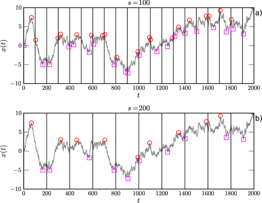
Figure 1: (Color online) An illustration of the extracted extreme points at different $s$ levels: a) $s=100$, and b) $s=200$. The local maxima and minima are demonstrated respectively by $\ocircle$ and $\square$. The vertical line indicates the window size $s$. To ensure spacial homogeneity, a sliding window with level $s$ scans over the whole data set, see more detail in the text.

At a specific $s$ level, denote the corresponding extremal point set as $x_{s,i}$, $i=1,2,...$ (along the coordinate increasing direction). Numerical tests show that typically these points are $\max-\min$ alternated for small $s$, while when $s$ increases $\max-\max$ or $\min-\min$ events may also appear but with low probability (e.g., $5\%$), depending on the $f(x)$ structure and the process physics. The segment is defined as the part of $f(x)$ between two adjacent extremal points. The characteristic parameters to describe the structure skeleton are the function difference, i.e., $f(x_{s,i})-f(x_{s,i-1})$ and the length scale, i.e., $\ell=x_{s,i}-x_{s,i-1}$. By varying the $s$ value, different extremal point sets, and thus different segment sets, can be obtained. In this sense this procedure is named as multi-level segment analysis (MSA); while the existing approaches based on local extremal points (Wang and Peters, 2006, 2008; Wang, 2014) calculate extrema from the DNS data; thus can be understood as single-level. Compared with the conventional SF, in MSA the segment length scale is not an independent input, but determined by $f(x)$.

For a specified $s$, scan over the data domain to have the corresponding segment characteristics, i.e. $f(x_{s,i})-f(x_{s,i-1})$ and $\ell=x_{s,i}-x_{s,i-1}$. Collect the results for different $s$, the functional statistics can be defined. Numerically the same segments may be counted repeatedly for different $s$, which then need to be excluded. In terms of structure function, the mathematical expression is (for the $q$th order case)

$$\mathcal{D}_{q}(\ell)=\langle[f(x_{s,i})-f(x_{s,i-1})]^{q}|{x_{s,i}-x_{s,i-1}=\ell}\rangle_{s},$$ (1)

where $\langle\cdot\rangle_{s}$ denotes sampling over different $s$. If any scaling relation exists, one may expect a power-law behavior as

$$\mathcal{D}_{q}(\ell)\sim\ell^{\xi(q)},$$ (2)

in which $\xi(q)$ is the MSA scaling exponent.

For comparison we also include here briefly the classical SF and wavelet-leader definitions. The $q$th order SF is written as

$$S_{q}(\ell)=\langle|\Delta x_{\ell}(t)|^{q}\rangle\sim\ell^{\zeta(q)},$$ (3)

where $\Delta x_{\ell}(t)=x(t+\ell)-x(t)$ and $\ell$ is the time separation scale. The scaling exponent $\zeta(q)$ characterizes the fluctuation statistics. $\zeta(q)$ is linear for monofractal processes such as fractional Brownian motion, and nonlinear and concave for multifractal processes (Schertzer et al., 1997). As mentioned above, SF mixes information from different scales. It is also limited by the slope of the Fourier spectrum $E(f)\sim f^{-\beta}$, e.g., $1<\beta<3$ (Frisch, 1995; Huang et al., 2010). We denote this as $\beta$-limitation.

There are several different wavelet-based methods, for example, wavelet-transform-modulus-maxima (WTMM) (Muzy et al., 1991; Mallat and Hwang, 1992; Muzy et al., 1993) and wavelet-leader (WL) (Jaffard et al., 2005; Wendt et al., 2007; Lashermes et al., 2008). We consider here only WL. More detailed discussions of those methods can refer to Ref. (Jaffard et al., 2005; Oświȩcimka et al., 2006; Huang et al., 2011) and references therein.
The discrete wavelet transform is defined as

$$\psi(k,j)=\int_{\mathbb{R}}x(t)\varphi\left(2^{-j}t-k\right)\mathrm{\,d}t,$$ (4)

where $\varphi$ is the chosen wavelet, $\psi(k,j)$ is the wavelet coefficient, $k$ is the position index, $j$ is the scale index, and $\ell=2^{j}$ is the corresponding scale (Daubechies, 1992; Mallat, 1999). Every discrete wavelet coefficient $\psi(k,j)$ can be associated with the dyadic interval $\varrho(k,j)$

$$\varrho(k,j)=[2^{j}k,2^{j}(k+1)).$$ (5)

Thus the wavelet coefficients can be represented as $\psi(\varrho)=\psi(k,j)$. The wavelet-leader is defined as

$$l(k,j)=\sup_{\varrho^{\prime}\subset 3\varrho(k,j),j^{\prime}\leq j}|\psi(\varrho^{\prime})|,$$ (6)

where $3\varrho(k,j)=\varrho(k-1,j)\cup\varrho(k,j)\cup\varrho(k+1,j)$ (Jaffard et al., 2005; Lashermes et al., 2008; Wendt et al., 2007). The expected scaling behavior can be expressed as

$$Z_{q}(j)=\langle l(k,j)^{q}\rangle\sim 2^{j\chi(q)},$$ (7)

in which $\chi(q)$ is the corresponding scaling exponent. The calculation efficiency has been discussed for various datasets (Jaffard et al., 2005; Wendt et al., 2007; Lashermes et al., 2008).

As shown in the rest of this paper, for simple cases, MSA and the classic methods show pretty identical results; while for complex analyses as turbulence, because of the algorithmic principle to depict the function structure, the former one is more effective and efficient.

Some additional comments are stated as follows. First, MSA can be considered as a dynamic-based approach without any basis assumption a priori. Since local extrema imply the change of the sign of $f^{\prime}(x)$ across $x_{s,i}$. Assuming that $f(x)$ represents a velocity signal, $f^{\prime}(x)$ is then the acceleration, i.e. a dynamical variable. Second, MSA shares the spirit of the wavelet-transform-modulus-maxima (WTMM) (Muzy et al., 1993), in which only the maximum modulus of the wavelet coefficient is considered. However, as argued in several Refs. (Huang et al., 1998, 2011), if the shape of the chosen mother wavelet is different with the specific turbulent structure, e.g., ramp-cliff in the passive scalar field, additional high-order harmonic components are then mixed to fit the difference between the physical structure and the mother wavelets, which then biases the extracted scaling (Huang et al., 2011). In this aspect MSA can be considered as a data-driven type of WTMM without any transform. Similar with the wavelet leader, Welter and Esquef (2013) proposed a multifractal analysis based on the amplitude extrema of intrinsic mode functions, which can be retrieved by the empirical mode decomposition algorithm (Huang et al., 1998). In some synthesized data tests, a proposed parameter $m=2$ is used to determine the search domain for the local amplitude maxima.

3 Case verification and applications

3.1 Fractional Brownian motion

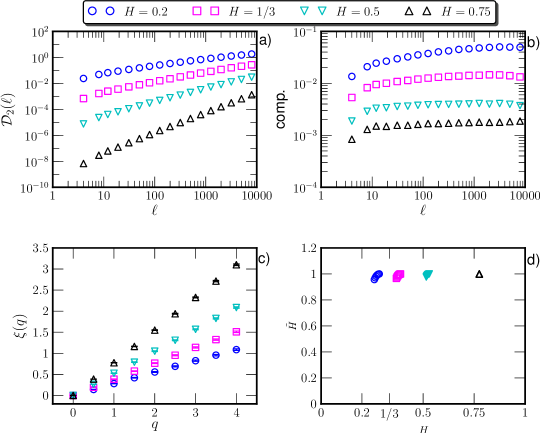
Figure 2: (Color online) a) Calculated second-order $\mathcal{D}_{2}(\ell)$ by MSA for fractional Brownian motion with Hurst number $H=0.2$ ($\ocircle$), $H=1/3$ ($\square$), $H=0.5$ ($\bigtriangledown$) and $H=0.75$ ($\triangle$), respectively. Power-law behavior can be observed for all $H$. b) Compensated curves $\mathcal{D}_{2}(\ell)\times\ell^{-2H}$. For display clarity, these curves have been vertical shifted. c) Experimental scaling exponents $\xi_{H}(q)$ in the range $0\leq q\leq 4$. The errorbar implies the standard deviation from 100 realizations. d) Measured singularity spectrum $f(\alpha)$.

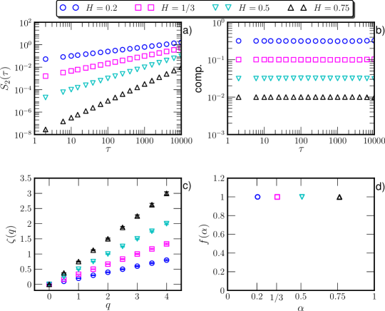
Figure 3: (Color online) Experimental results for the SF analysis: a) the measured second-order SFs $S_{2}(\tau)$; b) compensated curves $S_{2}(\tau)\times\tau^{-2H}$; c) measured scaling exponent $\zeta(q)$, and d) the measured singularity spectrum $f(\alpha)$ versus $\alpha$. Symbols are the same as in figure 2.

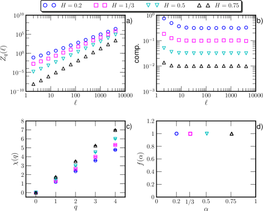
Figure 4: (Color online) Experimental results for the wavelet leader: a) the measured second-order $Z_{2}(\ell)$; b) compensated curves $Z_{2}(\ell)\times\tau^{-(2H+2)}$; c) measured scaling exponent $\chi(q)$, and d) the measured singularity spectrum $f(\alpha)$ versus $\alpha$. The symbols are the same as in figure 2.

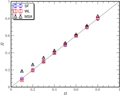
Figure 5: (Color online) Comparison of the measured Hurst number $\tilde{H}$ versus the given $H$. The theoretical value is indicated by the the solid line.

Fractional Brownian motion (fBm) is a generalization of the classical Brownian motion. It was introduced by Kolmogorov (1940) and extensively studied by Mandelbrot and co-workers in the 1960s (Mandelbrot and Van Ness, 1968). Since then, it is considered as a classical scaling stochastic process in many fields (Beran, 1994; Rogers, 1997; Doukhan et al., 2003). In the multifractal context, fBm is a simple self-similar process. More precisely, the measured SF scaling exponent $\zeta_{H}(q)$ is linear with the moment order $q$, i.e., $\zeta_{H}(q)=qH$, in which $H\in(0,1)$ is the Hurst number. The above linear scaling relation has been verified by various methodologies, such as, classical SF, wavelet-based method, detrended fluctuation analysis and detrended structure-function, to list a few. In the present work, a fast Fourier transform based Wood-Chan algorithm (Wood and Chan, 1994) is used to synthesize the fBm data with 100 realizations, and $10^{6}$ points for each $H$.

Figure 2 a) shows respectively the calculated second-order $\mathcal{D}_{2}(\ell)$ by MSA for Hurst number $H=0.2$ ($\ocircle$), $H=1/3$ ($\square$), $H=0.5$ ($\bigtriangledown$), and $H=0.75$ ($\triangle$). The power-law behavior is observed for all $H$ considered here. To emphasize the agreement between the measured $\xi_{H}(q)$ and the theoretical value, compensated curves of $\mathcal{D}_{2}(\ell)\ell^{-2H}$ are shown in figure  2 b). For display clarity, these curves have been vertical shifted. Visually, when $H<1/3$, the measured $\xi(q)$ deviates from the theoretical prediction. Such outcome may be related to MSA itself or the fBm date generation algorithm. Further investigation will be conducted hereof. Figure 2 c) shows the measured $\xi(q)$, which are estimated in the range $10<\ell<10,000$ by least-square-fitting. The errorbars indicate the standard deviation from 100 realizations (same in the following). These curves demonstrate for all the cases the linear dependence of the measured scaling exponent $\xi(q)$ with $q$, whose slope is $\tilde{H}$. In other words, multifractality can successfully be detected by MSA for all $H$ values (including $H<1/3$). Consider the so-called singularity spectrum, which is defined through a Legendre transform as,

$$\alpha=\frac{\mathrm{\,d}\xi(q)}{\mathrm{\,d}q},\quad f(\alpha)=\min_{q}\left\{\alpha q-\xi(q)+1\right\}.$$ (8)

For a monofractal process, $\alpha$ is independent with $q$, e.g., $\alpha=H$, and $f(\alpha)=1$ (Frisch, 1995). In practice, for a prescribed $q$, a wider range of $\alpha$ has, a more intermittent the process is. Figure 2 d) shows the measured $f(\alpha)$ in the range $0\leq q\leq 4$. It confirms the monofractal property of the fBm process.

Figure 3 lists the results from SF: a) the measured second-order SFs, $S_{2}(\tau)$, b) the compensated curves $S_{2}(\tau)\times\tau^{-2H}$, c) the measured scaling exponents $\zeta(q)$ and d) the corresponding singularity spectrum $f(\alpha)$ versus $\alpha$, respectively. Visually, a plateau is observed for all $\tau$, showing a perfect agreement between the detected scaling and theory. Here the scaling exponents $\zeta(q)$ are also estimated in the same the range $10<\tau<10,000$ by least-square-fitting. It shows that $\zeta(q)$ is linear with $q$, and the measured singularity spectrum $f(\alpha)$ detects correctly the monofractal property of the fBm process.

Figure 4 shows the results from the second-order WLs. Power-law behavior is observed for all $H$. Compensated curves $Z_{2}(\ell)\times\ell^{-(2H+2)}$ show a clear plateau when $\ell\geq 10$. Similar as MSA, misalignment is observed when $\ell<10$, which may be due to the fBm generator used in this study. Scaling exponents are then estimated in $10<\tau<10,000$. The measured $\chi(q)$ and the corresponding singularity spectrum $f(\alpha)$ capture the monofractal property of the fBm. Note that the singularity spectrum of WLs is defined as (Huang et al., 2011),

$$\alpha=\frac{\mathrm{\,d}\chi(q)}{\mathrm{\,d}q}-1,f(\alpha)=\min_{q}\left\{\alpha q-\chi(q)+1+q\right\}.$$ (9)

Figure 5 shows the comparison of the different estimated Hurst numbers $\tilde{H}$, which are calculated by linear fitting of the measured scaling exponent $\xi(q)$, $\zeta(q)$ and $\chi(q)$, respectively. Visually, SF and WL provide almost the same performance, while MSA slightly overestimates $H$ when $H>1/3$. All methods considered here confirm the monofractal property of the fBm process. Considering that the turbulent data are much different from the simple fBm, as already shown in Ref. Huang et al. (2011), both SF and WL are strongly influenced by the real turbulent structures.

We provide a comment here on the deviation of the measured $\xi(q)$ from the theoretical prediction when $H\leq 1/3$. In the context of extreme point based MSA, the intrinsic structure of fBm is presented by these extrema. Therefore how $\xi(q)$ will behave is determined by the relation between the Hurst number $H$ and the distribution of the extreme points, as well as the fBm data generation. Or in other words, the retrieved $\xi(q)$ relies on the dynamic behavior of the process itself, which is deeply related with the distribution of the extrema point. This is beyond the topic of this paper. We will present more details on this topic in the follow-up studies.

3.2 Lagrangian velocity

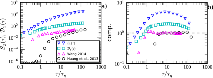
Figure 6: (Color online) a) Results from various methods: classical SF ($\bigtriangledown$) and the Hilbert-based method ($\ocircle$) for the second-order statistics, the trajectory-segment method ($\triangle$) and MSA $\mathcal{D}_{1}(\tau)$ ($\square$) for the first-order statistics. For the Hilbert-based statistics, frequency has been converted to time by $\tau=1/\omega$. b) The corresponding curves compensated by the dimensional scalings, i.e. $S_{2}(\tau)\sim\varepsilon\tau$ and $S_{1}(\tau)\sim(\varepsilon\tau)^{1/2}$. There is no plateau from SF, in consistency with other reports in the literature. The following convincing scaling ranges can be observed: about $2<\tau/\tau_{\eta}<60$ from MSA, $2<\tau/\tau_{\eta}<50$ from the trajectory segment analysis and $10<\tau/\tau_{\eta}<100$ from the Hilbert-based method, which verify the prediction of the Kolmogorov-Landau’s phenomenological theory. For display clarity, these curves have been vertical shifted.

The Lagrangian velocity SF has been extensively studied. Because the time scale separation in the Lagrangian frame is more Reynolds number dependent than the length scale case in the Eulerian frame, the finite Reynolds number influence becomes stronger, making the Lagrangian velocity scaling relation quite controversial (Falkovich et al., 2012). More specifically, this is recognized as a consequence of mixing between large-scale structures and energetic small-scale structures, e.g., vortex trapping events (Toschi et al., 2005; Huang et al., 2013). The $q$th-order SF of the velocity component $u_{i}\ (i=1,2,$ or $3)$ is defined as:

$$S_{q}(\tau)\equiv\langle[u_{i}(t+\tau)-u_{i}(t)]^{q}\rangle,$$ (10)

where $\tau$ is an arbitrary time separation scale. From dimensional analysis, the 2nd-order SF is supposed to satisfy (Falkovich et al., 2012):

$$S_{2}(\tau)=C_{0}\varepsilon\tau,$$ (11)

where $\varepsilon$ is the rate of energy dissipation per unit mass and $C_{0}$ is assumed as a universal constant at high Reynolds numbers.

To analyze this problem, we adopted the data from direct numerical simulation (DNS), implemented for the isotropic turbulence in a $2048^{3}$ cubic domain. The boundary conditions are periodic along each spatial direction and kinetic energy is continuously provided at few lowest wave number components. A fine resolution of $dx\sim\eta$ (the Kolmogorov scale) ensures resolving the detailed small-scale velocity dynamics. The Taylor scale $\lambda$ based Reynolds number $Re_{\lambda}$ is about $400$. Totally $0.2$ million Lagrangian particle samples are collected, each of which has about one integral time life span. During the evolution process, the velocity and velocity derivatives are recorded at each $\tau_{\eta}/20$, which $\tau_{\eta}$ is the Kolmogorov time. More numerical details can be found in Ref. Benzi et al. (2009) and references therein.

Recently, this database has been analyzed respectively by Huang et al. (2013), and Wang (2014) to identify the inertial scaling behavior. The former study employed the Hilbert-based approach, in which different scale events are separated by the empirical mode decomposition without any a priori basis assumption and the corresponding frequency $\omega$ is extracted by the Hilbert spectral analysis. They observed clearly an inertial range of $0.01<\omega\tau_{\eta}<0.1$, i.e. $10<\tau/\tau_{\eta}<100$. The scaling exponents $\zeta(q)$ agree well with the multifractal model (see details in Ref. Huang et al. (2013)). The latter one studies the extrema of the fluid particle acceleration, which physically can be considered as the boundary markers between different flow regions. With the help of the so-called trajectory segment structure, the clear scaling range does appear. Because of interpolation inaccuracy (noise), DNS data need to be particularly smoothed (Wang, 2014), which may lead to some artificial input.

Figure 6 a) shows the numerical results from various methods: classical SF ($\bigtriangledown$) and the Hilbert-based method ($\ocircle$) for the second-order statistics, the trajectory-segment method ($\triangle$) and MSA ($\square$) for the first-order statistics. Except for SF, clear power-law behaviors can be observed for others. To emphasize this, curves compensated by the dimensional scalings, i.e. $S_{2}(\tau)\sim\varepsilon\tau$ and $S_{1}(\tau)\sim(\varepsilon\tau)^{1/2}$, are plotted in Fig. 6 b). The SF curve does not show any plateau, which is consistent with reports in the literature (Falkovich et al., 2012; Sawford and Yeung, 2011), even for high $Re$ cases as $Re_{\lambda}\simeq 815$ experimentally or $Re_{\lambda}\simeq 1000$ numerically. The absence of the clear inertial range makes the Kolmogorov-Landau’s phenomenological theory quite controversial. In comparison, the MSA curve shows a convincing plateau in the range $2<\tau/\tau_{\eta}<60$.

It need to mention that for this DNS database the inertial range has been recognized as $10<\tau/\tau_{\eta}<100$ for both the single particle statistics using the Hilbert-based methodology (Huang et al., 2013) and the energy dissipation statistics to check the Lagrangian version refined similarity hypothesis (Huang and Schmitt, 2014). Here the inertial range $2<\tau/\tau_{\eta}<60$ detected by MSA is due to the different scale definition.

3.3 2D turbulence velocity field

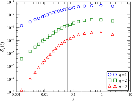
Figure 7: (Color online) Measured structure-function $S_{q}(\ell)$ for the two-dimensional turbulent velocity. Due to the scale-mixing in SF analysis, there is no power-law behavior.

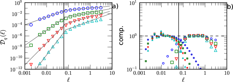
Figure 8: (Color online) a) Measured $q$th-order $\mathcal{D}_{q}(\ell)$ from MSA. A dual-cascade power-law behavior is observed in the range $0.004<\ell<0.04$ for the forward enstrophy cascade, and $0.15<\ell<1$ for the inverse energy cascade. b) The curves compensated by the least square fitted scaling exponent $\zeta(q)$ to emphasize the power-law behavior. The vertical solid line indicates the forcing scale $\ell_{f}=0.0614.$

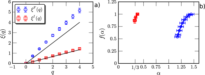
Figure 9: (Color online) a) Fitted scaling exponents $\xi(q)$ for both the forward enstrophy ($\ocircle$) and inverse energy ($\square$) cascades. The two solid lines represent respectively the Krainchan’s prediction $\xi(q)=q$ for the forward cascade and $\xi(q)=q/3$ for the inverse cascade. b) Measured singularity spectrum $f(\alpha)$. The inset shows the enlargement part in $0.2<\alpha<0.5$. A broader range of $1.17\leq\alpha\leq 1.45$ and $0.54\leq f(\alpha)\leq 1$ for the forward enstrophy cascade indicates a stronger intermittency.

Two-dimensional (2D) turbulence is an ideal model for the large scale movement of the ocean or atmosphere (Boffetta and Ecke, 2012; Kraichnan and Montgomery, 1980; Tabeling, 2002; Bouchet and Venaille, 2012). We recall here briefly the main theoretical results of 2D turbulence advocated by Kraichnan (1967).

The 2D Ekman-Navier-Stokes equation can be written as

$$\partial_{t}\mathbf{u}+\mathbf{u}\cdot\nabla\mathbf{u}=-\nabla p+\nu\bigtriangledown^{2}\mathbf{u}-\alpha\mathbf{u}+\mathbf{f}_{u},$$ (12)

in which $\mathbf{u}(\mathbf{x},t)=[u(\mathbf{x},t),v(\mathbf{x},t)]$ is the velocity vector, $\nu$ is the fluid viscosity, $\alpha$ is the Ekman friction and $\mathbf{f}_{u}$ is an external source of energy inputting into the whole system at scale $\ell_{\mathbf{f}}=1/k_{\mathbf{f}}$ (Boffetta, 2007). Parallelly, the vorticity $\omega=\nabla\times\mathbf{u}$ equation is

$$\partial_{t}\omega++\mathbf{u}\cdot\nabla\omega=\nu\bigtriangledown^{2}\omega-\alpha\omega+\mathbf{f}_{\omega}.$$ (13)

To keep the whole system balance, two conservation laws emerge. The first one is the so-called energy conservation, inducing an inverse energy cascade from the forcing scale $\ell_{\mathbf{f}}$ to large scales, i.e., $\ell>\ell_{\mathbf{f}}$, which then leads to a five-third law in the Fourier space above the forcing scale, i.e.,

$$E_{u}(k)=C\epsilon^{2/3}_{\alpha}k^{-5/3},\quad k_{\alpha}\ll k\ll k_{\mathbf{f}}\textrm{ for the inverse energy cascade},$$ (14)

where $E_{u}(k)$ is the Fourier power spectrum of $\mathbf{u}$, $\epsilon_{\alpha}$ is the energy dissipation by the Ekman friction, $k_{\alpha}$ is the Ekman friction scale and $k_{\mathbf{f}}=1/\ell_{\mathbf{f}}$ is the forcing scale. Below the forcing scale $\ell<\ell_{\mathbf{f}}$, the enstrophy conservation law yields

$$E_{u}(k)=C^{\prime}\eta^{2/3}_{\nu}k^{-3},\quad k_{\mathbf{f}}\ll k\ll k_{\nu}\textrm{ for the forward enstrophy cascade},$$ (15)

in which $\eta_{\nu}$ is the enstrophy dissipation by the viscosity $\nu$ and $k_{\nu}$ is the viscosity scale. This double-cascade 2D turbulence theory has been recognized as one of the most important results in turbulence since Kolmogorov’s 1941 work (Falkovich and Sreenivasan, 2006).

For the last few decades, numerous experiments and numerical simulations have been devoted to verify the above mentioned forward and inverse cascades (Bruneau and Kellay, 2005; Rutgers, 1998; Kellay et al., 1998; Bernard et al., 2006; Boffetta, 2007; Falkovich and Lebedev, 2011; Tan et al., 2014) with partially verification of the theory by Kraichnan. For example, Boffetta and Musacchio (2010) performed a very high resolution numerical simulation, up to a grid number $N=32,768^{2}$. They stated that due to the scale separation problem, numerically the dual-cascade requires a very high resolution for verification. The inverse and forward cascades were observed for the third-order velocity structure function as predicted by the theory (Boffetta and Musacchio, 2010, see Figure 3). For the inverse cascade, it is found that the inverse energy cascade is almost nonintermittent (Nam et al., 2000; Tan et al., 2014), while for the forward enstrophy cascade, the intermittency effect still remains as a open question. This is because, according to the convergency condition, the structure-function requires a Fourier spectrum $E(k)\sim k^{-\beta}$ with $\beta\in(1,3)$, the $\beta$-limitation (Huang et al., 2010). Coincidentally, the Fourier scaling exponent for the enstrophy cascade is $\beta\geq 3$, see equation (15) and discussion in Ref. Boffetta and Musacchio (2010). Theoretically, Nam et al. (2000) found that the Ekman friction leads to an intermittent forward enstrophy cascade (Bernard, 2000), which has been verified indirectly by studying the passive scalar field, instead of the vorticity field (Boffetta et al., 2002). More recently, this claim has been confirmed by Tan et al. (2014) using Hilbert spectral analysis. A log-Poisson model without justice is proposed to fit the forward enstrophy cascade scaling exponent, see detail in Ref. Tan et al. (2014). However, to identify whether the forward enstrophy cascade is intermittent or not is still a challenge in the sense of data analysis.

The DNS data for present analysis is based on a fully resolved vorticity field simulation (Boffetta, 2007), with an artificially added friction coefficient. Numerical integral of equation (13) is performed by a pseudo-spectral, fully dealiased on a doubly periodic square domain of size $L=2\pi$ with $N^{2}=8192^{2}$ grid points (Boffetta, 2007). The key parameters adopted are $\nu=2\times 10^{-6}$, $\alpha=0.025$ and the energy input wave number $k_{\mathbf{f}}=100$ with very short correlation in time. The velocity field is be solved from the Poisson equation of the stream function $\psi$, i.e., $\mathbf{u}=[\partial_{y}\psi,-\partial_{x}\psi]$. Totally, five snapshots with $8192^{2}\times 5=3.36\times 10^{8}$ data points are used for analysis. More details of this database can be found in Ref. Boffetta (2007).

The conventional SFs are shown in figure 7 and no clear scaling range can be observed, neither any indication of the aforementioned two regimes. As discussed above and also in Ref. Tan et al. (2014), such outcome can be ascribed to the scaling mixing in SF analysis (Huang et al., 2010). For comparison the results from MSA are shown in figure 8 a), in which two regimes with different scaling relations appear, specifically in the range $0.004<\ell<0.04$ for the forward enstrophy cascade and $0.15<\ell<1$ for the inverse energy cascade. To emphasize the observed power-law behavior, the compensated curves are then displayed in figure 8 b) by using the fitted scaling exponents $\xi(q)$. Two clear plateaus appear, confirming the existence of the dual-cascade process in the 2D turbulence. The scaling exponents $\xi(q)$ are then estimated in these scaling ranges by a least-square-fitting algorithm. Figure 9 a) shows the measured dual-cascade $\xi(q)$. The theoretical predictions by equations (14) (i.e. $q/3$) and (15) (i.e. $q$) are indicated by solid lines. Note that the measured forward cascade curve is larger than the theoretical one. A similar observation for the Fourier power spectrum has been reported in Ref. Boffetta (2007), which is considered as an influence of the fluid viscosity $\nu$.

To detect the multifractality, the singularity spectrum $f(\alpha)$ is then estimated, which is shown in figure 9 b). Based on the fBm case test, one can conclude that the inverse cascade is nonintermittent as expected; while the forward enstrophy cascade shows a clear sign of multifractality: a broad change of $\alpha$ and $f(\alpha)$. Note that $\alpha$ is the generalized Hurst number. The value range $\alpha\in(1.17,1.45)$ implies a Hurst number $H>1$, much larger than the one indicated by the equation (15), i.e., $H=1$. Such outcome may be an effect of the logarithmic correction (Pasquero and Falkovich, 2002), while it is reported by Tan et al. (2014) that the logarithmic correlation for the vorticity field is weak. It also has to point out here that the measured $\alpha$ and $f(\alpha)$ could be a function of $\nu$ or the Ekman friction (Boffetta, 2007; Boffetta and Ecke, 2012; Tan et al., 2014). Systematic analysis of the 2D velocity field with different parameter is necessary in the future for deeper insights.

4 Discussion and Conclusions

In summary, we propose in this paper a multiscale statistical method, namely multi-level segment analysis, without employing any decomposition. The statistical properties of extremal points at multiple $s$ level inherit the intrinsic multi-scale physics of complex systems. For each $s$, the corresponding extremal point series defines the so-called segment, which can be characterized by the separation distance and the function difference at adjacent extrema. As an important extension of the existing work, the MSA method introduced in this paper proves meaningful in complex data analysis. This new approach has been verified by revealing the monofractal property of the synthesized fBm processes, while the Hurst number $H$ is slightly overestimated especially when $H<1/3$. When applied to two numerical turbulent datasets, i.e. the high-resolution Lagrangian 2D turbulence, MSA shows interesting outcome. The conventional methodologies, such as SF, fail to detect the inertial scaling of the velocity field, which is now recognized partially as the $\beta$-limitation, and partially as contamination by the energetic structures (Huang et al., 2013). Very differently, MSA detects successfully the clear scaling ranges for both cases. More precisely for 2D turbulence, the retrieved multifractal property of the forward enstrophy confirms the theoretical prediction by Nam et al. (2000). More systematic study of such multifractality and parametric dependance (e.g. the fluid viscosity) is important in future to provide a better understanding of 2D turbulence.

Finally, we provide the following general remarks:

• In principle, MSA is generally applicable without special requirements on the data itself, such as periodicity, the Fourier spectrum slope $\beta$ ( steeper than $3$), noise perturbation and unsmoothness structures.

• The length scale in the context of MSA is determined by the functional structure rather than being an independent input. At different $s$ levels the segments are different and thus the scales as well, which conforms with the multi-scale physics.

• A serious deficiency of the conventional SF is the strong mixing of different correlation and scaling regimes due to sample averaging, i.e. the filtering (as infrared and ultraviolet) effect. To define the segment structure helps to annihilate such filtering and extract the possible scaling relations in the respective scale regimes, which has been proved from analyzing the Lagrangian and 2D turbulence data.

• Moreover irregular sampling (e.g. missed points) is a common problem for data collection as in the geophysical experiments, LDV (Laser Doppler Velocimetry) measurement, etc. However, typically methods as Fourier analysis and others require uniform spacial data points. Such trouble is easy to overcome in MSA since only extremal instead of all the functional points are involved.

References

- (1)
- Benzi et al. (2009) Benzi R, Biferale L, Calzavarini E, Lohse D and Toschi F 2009 Phys. Rev. E 80(6), 066318.
- Beran (1994) Beran J 1994 Statistics for long-memory processes CRC Press.
- Bernard (2000) Bernard D 2000 EPL (Europhysics Letters) 50, 333.
- Bernard et al. (2006) Bernard D, Boffetta G, Celani A and Falkovich G 2006 Nature Phys. 2(2), 124–128.
- Boffetta (2007) Boffetta G 2007 J. Fluid Mech. 589, 253–260.
- Boffetta et al. (2002) Boffetta G, Celani A, Musacchio S and Vergassola M 2002 Phys. Rev. E 66(2), 026304.
- Boffetta and Ecke (2012) Boffetta G and Ecke R 2012 Annu. Rev. Fluid Mech 44, 427–51.
- Boffetta and Musacchio (2010) Boffetta G and Musacchio S 2010 Phys. Rev. E 82(1), 016307.
- Bouchet and Venaille (2012) Bouchet F and Venaille A 2012 Phys. Rep. 515, 227–95.
- Bruneau and Kellay (2005) Bruneau C H and Kellay H 2005 Phys. Rev. E 71(4), 046305.
- Daubechies (1992) Daubechies I 1992 Ten lectures on wavelets Philadelphia: SIAM.
- Davidson and Pearson (2005) Davidson P A and Pearson B R 2005 Phys. Rev. Lett. 95, 214501.
- Doukhan et al. (2003) Doukhan P, Taqqu M and Oppenheim G 2003 Theory and Applications of Long-Range Dependence Birkhauser, Berlin.
- Falkovich and Lebedev (2011) Falkovich G and Lebedev V 2011 Phys. Rev. E 83(4), 045301.
- Falkovich and Sreenivasan (2006) Falkovich G and Sreenivasan K R 2006 Phys. Today 59, 43.
- Falkovich et al. (2012) Falkovich G, Xu H, Pumir A, Bodenschatz E, Biferale L, Boffetta G, Lanotte A and Toschi F 2012 Phys. Fluids 24(4), 055102.
- Farge (1992) Farge M 1992 Annu. Rev. Fluid Mech. 24(1), 395–457.
- Farge et al. (1996) Farge M, Kevlahan N, Perrier V and Goirand E 1996 IEEE J PROC 84(4), 639–669.
- Frisch (1995) Frisch U 1995 Turbulence: the legacy of AN Kolmogorov Cambridge University Press.
- Huang et al. (1998) Huang N, Shen Z, Long S, Wu M, Shih H, Zheng Q, Yen N, Tung C and Liu H 1998 Proc. R. Soc. London, Ser. A 454(1971), 903–995.
- Huang (2014) Huang Y 2014 J. Turb. 15(4), 209–220.
- Huang et al. (2013) Huang Y, Biferale L, Calzavarini E, Sun C and Toschi F 2013 Phys. Rev. E 87, 041003(R).
- Huang and Schmitt (2014) Huang Y and Schmitt F G 2014 J. Fluid Mech. 741, R2.
- Huang et al. (2011) Huang Y, Schmitt F G, Hermand J P, Gagne Y, Lu Z and Liu Y 2011 Phys. Rev. E 84(1), 016208.
- Huang et al. (2010) Huang Y, Schmitt F G, Lu Z, Fougairolles P, Gagne Y and Liu Y 2010 Phys. Rev. E 82(2), 026319.
- Huang et al. (2008) Huang Y, Schmitt F G, Lu Z and Liu Y 2008 Europhys. Lett. 84, 40010.
- Huang et al. (2009) Huang Y, Schmitt F G, Lu Z and Liu Y 2009 J. Hydrol. 373, 103–111.
- Huang et al. (2011) Huang Y, Schmitt F G, Zhou Q, Qiu X, Shang X, Lu Z and Liu Y 2011 Phys. Fluids 23, 125101.
- Jaffard et al. (2005) Jaffard S, Lashermes B and Abry P 2005 Wavelet Analysis and Applications .
- Kellay et al. (1998) Kellay H, Wu X and Goldburg W 1998 Phys. Rev. Lett. 80(2), 277–280.
- Kolmogorov (1940) Kolmogorov A N 1940 Dokl. Akad. Nauk SSSR 26(2), 115–118.
- Kolmogorov (1941) Kolmogorov A N 1941 Dokl. Akad. Nauk SSSR 30, 301.
- Kraichnan (1967) Kraichnan R 1967 Phys. Fluids 10, 1417–1423.
- Kraichnan and Montgomery (1980) Kraichnan R and Montgomery D 1980 Rep.Prog. Phys. 43, 547.
- Lashermes et al. (2008) Lashermes B, Roux S, Abry P and Jaffard S 2008 Eur. Phys. J. B 61(2), 201–215.
- Li and Huang (2014) Li M and Huang Y 2014 Physica A 406, 222–229.
- Lovejoy and Schertzer (2012) Lovejoy S and Schertzer D 2012 Nonlinear Processes in Geophysics 19(5), 513–527.
- Mallat (1999) Mallat S 1999 A wavelet tour of signal processing Academic Pr.
- Mallat and Hwang (1992) Mallat S and Hwang W 1992 IEEE Transactions on Information Theory 38(2), 617–643.
- Mandelbrot and Van Ness (1968) Mandelbrot B and Van Ness J 1968 SIAM Review 10, 422.
- Mantegna and Stanley (1996) Mantegna R and Stanley H 1996 Nature 383(6601), 587–588.
- Muzy et al. (1991) Muzy J, Bacry E and Arneodo A 1991 Phys. Rev. Lett. 67(25), 3515–3518.
- Muzy et al. (1993) Muzy J, Bacry E and Arneodo A 1993 Phys. Rev. E 47(2), 875–884.
- Nam et al. (2000) Nam K, Ott E, Antonsen Jr T and Guzdar P 2000 Phys. Rev. Lett. 84(22), 5134–5137.
- Oświȩcimka et al. (2006) Oświȩcimka P, Kwapień J and Drożdż S 2006 Phys. Rev. E 74(1), 16103.
- Pasquero and Falkovich (2002) Pasquero C and Falkovich G 2002 Phys. Rev. E 65(5), 56305.
- Peng et al. (1994) Peng C, Buldyrev S, Havlin S, Simons M, Stanley H and Goldberger A 1994 Phys. Rev. E 49(2), 1685–1689.
- Qiu et al. (2014) Qiu X, Huang Y, Zhou Q and Sun C 2014 J. Hydrodyn. 26(3), 351–362.
- Rogers (1997) Rogers L 1997 Math. Finance 7(1), 95–105.
- Rutgers (1998) Rutgers M A 1998 Phys. Rev. Lett. 81(11), 2244.
- Sawford and Yeung (2011) Sawford B and Yeung P 2011 Phys. Fluids 23, 091704.
- Schertzer et al. (1997) Schertzer D, Lovejoy S, Schmitt F G, Chigirinskaya Y and Marsan D 1997 Fractals 5(3), 427–471.
- Schmitt et al. (1999) Schmitt F G, Schertzer D and Lovejoy S 1999 Appl. Stoch. Models and Data Anal. 15(1), 29–53.
- Schmitt et al. (1998) Schmitt F G, Vannitsem S and Barbosa A 1998 J. Geophys. Res. 103(D18), 23181–23193.
- Seuront et al. (1999) Seuront L, Schmitt F G, Lagadeuc Y, Schertzer D and Lovejoy S 1999 J. Plankton Res. 21(5), 877–822.
- Tabeling (2002) Tabeling P 2002 Phys. Rep. 362(1), 1–62.
- Tan et al. (2014) Tan H, Huang Y and Meng J P 2014 Phys. Fluids 26(2), 015106.
- Toschi et al. (2005) Toschi F, Biferale L, Boffetta G, Celani A, Devenish B and Lanotte A 2005 J. Turbu. 6(6), 15.
- Wang (2014) Wang L 2014 Phys. Fluids 26(4), 045104.
- Wang and Peters (2006) Wang L and Peters N 2006 J. Fluid Mech. 554, 457–475.
- Wang and Peters (2008) Wang L and Peters N 2008 J. Fluid Mech. 608, 113–138.
- Wang and Peters (2013) Wang L and Peters N 2013 Philosophical Transactions of the Royal Society A 371(1982), 20120169.
- Welter and Esquef (2013) Welter G S and Esquef P A 2013 Phys. Rev. E 87(3), 032916.
- Wendt et al. (2007) Wendt H, Abry P and Jaffard S 2007 IEEE Signal Processing Mag. 24(4), 38–48.
- Wood and Chan (1994) Wood A and Chan G 1994 J. Comput. Graph. Stat. 3(4), 409–432.