Abstract

Reaching a theoretical accuracy in the prediction of the lightest MSSM Higgs-boson mass, $M_{h}$, at the level of the current experimental precision requires the inclusion of momentum-dependent contributions at the two-loop level. Recently two groups presented the two-loop QCD momentum-dependent corrections to $M_{h}$ [1, 2], using a hybrid on-shell–$\overline{\mathrm{DR}}$ scheme, with apparently different results. We show that the differences can be traced back to a different renormalization of the top-quark mass, and that the claim in Ref. [2] of an inconsistency in Ref. [1] is incorrect. We furthermore compare consistently the results for $M_{h}$ obtained with the top-quark mass renormalized on-shell and $\overline{\mathrm{DR}}$. The latter calculation has been added to the FeynHiggs package and can be used to estimate missing higher-order corrections beyond the two-loop level.

1 Introduction

The particle discovered in the Higgs-boson searches by ATLAS [3] and CMS [4] at CERN shows, within experimental and theoretical uncertainties, properties compatible with the Higgs boson of the Standard Model (SM) [5, 6, 7]. It can also be interpreted as the Higgs boson of extended models, however, where the lightest Higgs boson of the Minimal Supersymmetric Standard Model (MSSM) [8] is a prime candidate.

The Higgs sector of the MSSM with two scalar doublets accommodates five physical Higgs bosons. In lowest order these are the light and heavy ${\cal CP}$-even $h$ and $H$, the ${\cal CP}$-odd $A$, and the charged Higgs bosons $H^{\pm}$. At tree level, the Higgs sector can be parameterized in terms of the gauge couplings, the mass of the ${\cal CP}$-odd Higgs boson, $M_{A}$, and $\tan\beta\equiv v_{2}/v_{1}$, the ratio of the two vacuum expectation values; all other masses and mixing angles follow as predictions.

Higher-order contributions can give large corrections to the tree-level relations  [9, 10], and in particular to the mass of the lightest Higgs boson, $M_{h}$. For the MSSM with real parameters the status of higher-order corrections to the masses and mixing angles in the neutral Higgs sector is quite advanced, see Refs. [16, 17, 18, 19] for the calculations of the full one-loop level. At the two-loop level [20, 21, 22, 23, 24, 25, 26, 27, 28, 29, 30, 31, 32, 33, 34, 15] in particular the ${\cal O}(\alpha_{t}\alpha_{s})$ and ${\cal O}(\alpha_{t}^{2})$ contributions ($\alpha_{t}\equiv h_{t}^{2}/(4\pi)$, $h_{t}$ being the top-quark Yukawa coupling) to the self-energies – evaluated in the Feynman-diagrammatic (FD) as well as in the effective potential (EP) method – as well as the ${\cal O}(\alpha_{b}\alpha_{s})$, ${\cal O}(\alpha_{t}\alpha_{b})$ and ${\cal O}(\alpha_{b}^{2})$ contributions – evaluated in the EP approach – are known for vanishing external momenta. An evaluation of the momentum dependence at the two-loop level in a pure $\overline{\mathrm{DR}}$ calculation was presented in Ref. [35]. The latest status of the momentum-dependent two-loop corrections will be discussed below. A (nearly) full two-loop EP calculation, including even the leading three-loop corrections, has also been published [36]. Within the EP method all contributions are evaluated at zero external momentum, however, in contrast to the FD method which in principle allows for non-vanishing external momenta. Furthermore, the calculation presented in Ref. [36] is not publicly available as a computer code for Higgs-boson mass calculations. Subsequently, another leading three-loop calculation of ${\cal O}(\alpha_{t}\alpha_{s}^{2})$, depending on the various SUSY mass hierarchies, was completed [37], resulting in the code H3m which adds the three-loop corrections to the FeynHiggs [38, 21, 39, 11, 40] result. Most recently, a combination of the full one-loop result, supplemented with leading and subleading two-loop corrections evaluated in the FD/EP method and a resummation of the leading and subleading logarithmic corrections from the scalar-top sector has been published [40] in the latest version of the code FeynHiggs.

The measured mass value of the observed Higgs-boson is currently known to about $250\,\,\mathrm{MeV}$ accuracy [5], reaching the level of a precision observable. At a future linear collider (ILC), the precise determination of the light Higgs-boson properties and/or heavier MSSM Higgs-bosons within the kinematic reach will be possible [41]. In particular, a mass measurement of the light Higgs-boson with an accuracy below $\sim 0.05\,\,\mathrm{GeV}$ is anticipated [42].

In Ref. [39] the remaining theoretical uncertainty in the calculation of $M_{h}$, from unknown higher-order corrections, was estimated to be up to $3\,\,\mathrm{GeV}$, depending on the parameter region; see also Refs. [40, 43] for updated results. As the accuracy of the $M_{h}$ prediction should at least match the one of the experimental result, higher-order corrections which do not dominate the size of the Higgs-boson mass values have to be included in the Higgs-boson mass predictions.

To better control the size of momentum-dependent contributions, we recently presented the calculation of the ${\cal O}(p^{2}\alpha_{t}\alpha_{s})$ corrections to $M_{h}$ (the leading momentum-dependent two-loop QCD corrections). The calculation was performed in a hybrid on-shell/$\overline{\mathrm{DR}}$ scheme [1] at the two-loop level, where $M_{A}$ and the tadpoles are renormalized on-shell (OS), whereas the Higgs-boson fields and $\tan\beta$ are renormalized $\overline{\mathrm{DR}}$. At the one-loop level the top/stop parameters are renormalized OS. Subsequently, in Ref. [2] this calculation was repeated with a different result (also, a calculation in a pure $\overline{\mathrm{DR}}$ scheme as well as the two-loop corrections of ${\cal O}(\alpha\alpha_{s})$ were presented). Within Ref. [2] the discrepancy between Refs. [1] and [2] was explained by an inconsistency in the renormalization scheme used for the Higgs-boson field renormalization in Ref. [1].

In this paper we demonstrate that this claim is incorrect. The renormalization scheme for the Higgs-boson fields used in Ref. [1] is (up to corrections beyond the two-loop level) identical to the one employed in Ref. [2]. We clarify that the differences between the two results originates in a difference of the top-quark-mass renormalization scheme. While in Ref. [1] a full OS renormalization was used, in Ref. [2] the contributions to the top-quark self-energy of ${\cal O}(\varepsilon)$ (with $4-D=2\varepsilon$, $D$ being the space-time dimension) were neglected, leading to the observed numerical differences. We also demonstrate how this difference in the treatment of the contributions from the top quark mass can be linked to a difference in the two-loop field renormalization constant and explain why this difference should be regarded as a theoretical uncertainty at the two-loop level, which would be fixed only at three loop order.

We further present a consistent calculation of the ${\cal O}(p^{2}\alpha_{t}\alpha_{s})$ corrections to $M_{h}$ in a scheme where the top quark is renormalized $\overline{\mathrm{DR}}$, whereas the scalar tops continue to be renormalized OS. This new scheme is available from FeynHiggs version 2.11.1 on, allowing for an improved estimate of (some) unknown higher-order corrections beyond the two-loop level originating from the top/stop sector.

The paper is organized as follows. An overview of the relevant sectors and the renormalization employed in our calculation is given in Sect. 2. In Sect. 3 we compare analytically and numerically the results of Refs. [1] and [2]. Results obtained using the $\overline{\mathrm{DR}}$ scheme for the top-quark mass are given in Sect. 4. Our conclusions are given in Sect. 5.

2 The relevant sectors and their renormalization

2.1 The Higgs-boson sector of the MSSM

The MSSM requires two scalar doublets, which are conventionally written in terms of their components as follows,

$${\cal H}_{1} =\left(\begin{array}[]{c}{\cal H}_{1}^{0}\\[2.15277pt] {\cal H}_{1}^{-}\end{array}\right)=\left(\begin{array}[]{c}v_{1}+\frac{1}{\sqrt{2}}(\phi_{1}^{0}-i\chi_{1}^{0})\\[2.15277pt] -\phi_{1}^{-}\end{array}\right)\,,$$

$${\cal H}_{2} =\left(\begin{array}[]{c}{\cal H}_{2}^{+}\\[2.15277pt] {\cal H}_{2}^{0}\end{array}\right)=\left(\begin{array}[]{c}\phi_{2}^{+}\\[2.15277pt] v_{2}+\frac{1}{\sqrt{2}}(\phi_{2}^{0}+i\chi_{2}^{0})\end{array}\right)\,.$$

The bilinear part of the Higgs potential leads to the tree-level mass matrix for the neutral ${\cal CP}$-even Higgs-bosons,

$$M_{\text{Higgs}}^{2,\text{tree}}=\left(\begin{array}[]{cc}m_{\phi_{1}}^{2}&m_{\phi_{1}\phi_{2}}^{2}\\ m_{\phi_{1}\phi_{2}}^{2}&m_{\phi_{2}}^{2}\end{array}\right)=\left(\begin{array}[]{cc}M_{A}^{2}\sin^{2}\!\beta+M_{Z}^{2}\cos^{2}\!\beta&-(M_{A}^{2}+M_{Z}^{2})\sin\beta\cos\beta\\ -(M_{A}^{2}+M_{Z}^{2})\sin\beta\cos\beta&M_{A}^{2}\cos^{2}\!\beta+M_{Z}^{2}\sin^{2}\!\beta\end{array}\right),$$ (5)

in the $(\phi_{1},\phi_{2})$ basis, expressed in terms of the $Z$ boson mass, $M_{Z}$, $M_{A}$ and the angle $\beta$. Diagonalization via the angle $\alpha$ yields the tree-level masses $m_{h,{\rm tree}}$ and $m_{H,{\rm tree}}$. Below we also use $M_{W}$, denoting the $W$ boson mass and $s_{\mathrm{w}}$, the sine of the weak mixing angle, $s_{\mathrm{w}}=\sqrt{1-c_{\mathrm{w}}^{2}}=\sqrt{1-M_{W}^{2}/M_{Z}^{2}}$.

The higher-order-corrected ${\cal CP}$-even Higgs-boson masses in the MSSM are obtained from the corresponding propagators dressed by their self-energies. The calculation of these and their renormalization is performed in the $(\phi_{1},\phi_{2})$ basis, which has the advantage that the mixing angle $\alpha$ does not appear and expressions are in general simpler. The inverse propagator matrix in the $(\phi_{1},\phi_{2})$ basis is given by

$$(\Delta_{\text{Higgs}})^{-1}=-\text{i}\left(\begin{matrix}p^{2}-m_{\phi_{1}}^{2}+\hat{\Sigma}_{\phi_{1}}(p^{2})&-m_{\phi_{1}\phi_{2}}^{2}+\hat{\Sigma}_{\phi_{1}\phi_{2}}(p^{2})\\ -m_{\phi_{1}\phi_{2}}^{2}+\hat{\Sigma}_{\phi_{1}\phi_{2}}(p^{2})&p^{2}-m_{\phi_{2}}^{2}+\hat{\Sigma}_{\phi_{2}}(p^{2})\end{matrix}\right),$$ (6)

where $\hat{\Sigma}(p^{2})$ denote the renormalized Higgs-boson self-energies, $p$ being the external momentum. The renormalized self-energies can be expressed through the unrenormalized self-energies, $\Sigma(p^{2})$, and counterterms involving renormalization constants $\delta m^{2}$ and $\delta Z$ from parameter and field renormalization. With the self-energies expanded up to two-loop order, $\hat{\Sigma}=\hat{\Sigma}^{(1)}+\hat{\Sigma}^{(2)}$, one has for the ${\cal CP}$-even part at the $i$-loop level ($i=1,2$),

$$\hat{\Sigma}_{\phi_{1}}^{(i)}(p^{2}) =\,\Sigma_{\phi_{1}}^{(i)}(p^{2})+\delta Z_{\phi_{1}}^{(i)}\,(p^{2}-m_{\phi_{1}}^{2})-\delta m_{\phi_{1}}^{2(i)}~{},$$ (7a)

$$\hat{\Sigma}_{\phi_{1}\phi_{2}}^{(i)}(p^{2}) =\,\Sigma_{\phi_{1}\phi_{2}}^{(i)}(p^{2})-\delta Z_{\phi_{1}\phi_{2}}^{(i)}\,m_{\phi_{1}\phi_{2}}^{2}-\delta m_{\phi_{1}\phi_{2}}^{2(i)}~{},$$ (7b)

$$\hat{\Sigma}_{\phi_{2}}^{(i)}(p^{2}) =\,\Sigma_{\phi_{2}}^{(i)}(p^{2})+\delta Z_{\phi_{2}}^{(i)}\,(p^{2}-m_{\phi_{2}}^{2})-\delta m_{\phi_{2}}^{2(i)}~{}.$$ (7c)

At the two-loop level the expressions in Eqs. (7) do not contain contributions of the type (1-loop) $\times$ (1-loop); such terms do not appear at ${\cal O}(\alpha_{t}\alpha_{s})$ and hence can be omitted in the context of this paper. For the general expressions see Ref. [15].

Beyond the one-loop level, unrenormalized self-energies contain sub-loop renormalizations. At the two-loop level, these are one-loop diagrams with counterterm insertions at the one-loop level.

2.2 Renormalization

The following section summarizes the renormalization worked out in Ref. [1], based on Ref. [21]. The field renormalization is carried out by assigning one renormalization constant to each doublet,

$${\cal H}_{1}\to(1+\tfrac{1}{2}\delta Z_{{\cal H}_{1}})\,{\cal H}_{1},\quad{\cal H}_{2}\to(1+\tfrac{1}{2}\delta Z_{{\cal H}_{2}}){\cal H}_{2}\,,$$ (8)

which can be expanded to one- and two-loop order according to

$$\delta Z_{{\cal H}_{1}} =\,\delta Z_{{\cal H}_{1}}^{(1)}+\delta Z_{{\cal H}_{1}}^{(2)}\,,\quad\delta Z_{{\cal H}_{2}}\,=\,\delta Z_{{\cal H}_{2}}^{(1)}+\delta Z_{{\cal H}_{2}}^{(2)}\,.$$ (9)

The field renormalization constants appearing in (7) are then given by

$$\delta Z_{\phi_{1}}^{(i)}=\delta Z_{{\cal H}_{1}}^{(i)}\,,\quad\delta Z_{\phi_{2}}^{(i)}=\delta Z_{{\cal H}_{2}}^{(i)}\,,\quad\delta Z_{\phi_{1}\phi_{2}}^{(i)}=\tfrac{1}{2}(\delta Z_{{\cal H}_{1}}^{(i)}+\delta Z_{{\cal H}_{2}}^{(i)})\,.$$ (10)

The mass counterterms $\delta m^{2(i)}_{ab}$ in Eq. (7) are derived from the Higgs potential, including the tadpoles, by the following parameter renormalization,

$$M_{A}^{2} \to M_{A}^{2}+\delta M_{A}^{2(1)}+\delta M_{A}^{2(2)}, T_{1} \to T_{1}+\delta T_{1}^{(1)}+\delta T_{1}^{(2)},$$ (11)

$$M_{Z}^{2} \to M_{Z}^{2}+\delta M_{Z}^{2(1)}+\delta M_{Z}^{2(2)}, T_{2} \to T_{2}+\delta T_{2}^{(1)}+\delta T_{2}^{(2)},$$

$$\tan\beta \to\tan\beta\left(1+\delta\tan\beta^{(1)}+\delta\tan\beta^{(2)}\right)~{}.$$

The parameters $T_{1}$ and $T_{2}$ are the terms linear in $\phi_{1}$ and $\phi_{2}$ in the Higgs potential. The renormalization of the $Z$-mass $M_{Z}$ does not contribute to the $\mathcal{O}(\alpha_{s}\alpha_{t})$ corrections we are pursuing here; it is listed for completeness only.

The basic renormalization constants for parameters and fields have to be fixed by renormalization conditions according to a renormalization scheme. Here we choose the on-shell scheme for the parameters and the $\overline{\rm{DR}}$ scheme for field renormalization and give the expressions for the two-loop part. This is consistent with the renormalization scheme used at the one-loop level.

The tadpole coefficients are chosen to vanish at all orders; hence their two-loop counterterms follow from

$$T_{1,2}^{(2)}+\delta T_{1,2}^{(2)}=0\,,\quad\text{i.e.\ }\quad\delta T_{1}^{(2)}=-{T_{1}^{(2)}},\quad\delta T_{2}^{(2)}=-{T_{2}^{(2)}}\,,$$ (12)

where $T_{1}^{(2)}$, $T_{2}^{(2)}$ are obtained from the two-loop tadpole diagrams. The two-loop renormalization constant of the $A$-boson mass reads

$$\delta M_{A}^{2(2)}=\mathop{\mathrm{Re}}\Sigma_{AA}^{(2)}(M_{A}^{2}),$$ (13)

in terms of the $A$-boson unrenormalized self-energy $\Sigma_{AA}$. The appearance of a non-zero momentum in the self-energy goes beyond the ${\cal O}(\alpha_{t}\alpha_{s})$ corrections evaluated in Refs. [20, 21, 26].

For the renormalization constants $\delta Z_{{\cal H}_{1}}$, $\delta Z_{{\cal H}_{2}}$ and $\delta\tan\beta$ several choices are possible, see the discussion in [47]. As shown there, the most convenient choice is a $\overline{\rm{DR}}$ renormalization of $\delta\tan\beta$, $\delta Z_{{\cal H}_{1}}$ and $\delta Z_{{\cal H}_{2}}$, which at the two-loop level reads

$$\delta Z_{{\cal H}_{1}}^{(2)} =\delta Z_{{\cal H}_{1}}^{\overline{\mathrm{DR}}(2)}\;=\;-\left[\mathop{\mathrm{Re}}\Sigma^{\prime(2)}_{\phi_{1}}\right]^{\text{div}}_{|p^{2}=0}\,,$$ (14a)

$$\delta Z_{{\cal H}_{2}}^{(2)} =\delta Z_{{\cal H}_{2}}^{\overline{\mathrm{DR}}(2)}\;=\;-\left[\mathop{\mathrm{Re}}\Sigma^{\prime(2)}_{\phi_{2}}\right]^{\text{div}}_{|p^{2}=0}\,,$$ (14b)

$$\delta\tan\beta^{(2)} =\delta\tan\beta^{\overline{\mathrm{DR}}(2)}\;=\;\tfrac{1}{2}\left(\delta Z_{{\cal H}_{2}}^{(2)}-\delta Z_{{\cal H}_{1}}^{(2)}\right)\,.$$ (14c)

The term in Eq. (14c) is in general not the proper expression beyond one-loop order even in the $\overline{\rm{DR}}$ scheme. For our approximation, however, with only the top Yukawa coupling at the two-loop level, it is the correct $\overline{\rm{DR}}$ form [48].

The two-loop mass counterterms in the renormalized self-energies (7) are now expressed in terms of the two-loop parameter renormalization constants, determined above, as follows,

$$\delta m_{\phi_{1}}^{2(2)} =\,\delta M_{Z}^{2(2)}\,\cos^{2}\!\beta+\delta M_{A}^{2(2)}\sin^{2}\!\beta$$ (15a)

$$\quad-\delta T_{1}^{(2)}\frac{e}{2M_{W}s_{\mathrm{w}}}\,\cos\beta(1+\sin^{2}\!\beta)+\delta T_{2}^{(2)}\frac{e}{2M_{W}s_{\mathrm{w}}}\,\cos^{2}\!\beta\sin\beta$$

$$\quad+2\,\delta\tan\beta^{(2)}\,\cos^{2}\!\beta\sin^{2}\!\beta\,(M_{A}^{2}-M_{Z}^{2})\,,$$

$$\delta m_{\phi_{1}\phi_{2}}^{2(2)} =-(\delta M_{Z}^{2(2)}+\delta M_{A}^{2(2)})\sin\beta\cos\beta$$ (15b)

$$\quad-\delta T_{1}^{(2)}\frac{e}{2M_{W}s_{\mathrm{w}}}\,\sin^{3}\!\beta-\delta T_{2}^{(2)}\frac{e}{2M_{W}s_{\mathrm{w}}}\,\cos^{3}\!\beta$$

$$\quad-\delta\tan\beta^{(2)}\,\cos\beta\sin\beta\cos 2\beta\,(M_{A}^{2}+M_{Z}^{2})\,,$$

$$\delta m_{\phi_{2}}^{2(2)} =\delta M_{Z}^{2(2)}\sin^{2}\!\beta+\delta M_{A}^{2(2)}\cos^{2}\!\beta$$ (15c)

$$\quad+\delta T_{1}^{(2)}\frac{e}{2M_{W}s_{\mathrm{w}}}\,\sin^{2}\!\beta\cos\beta-\delta T_{2}^{(2)}\frac{e}{2M_{W}s_{\mathrm{w}}}\,\sin\beta(1+\cos^{2}\!\beta)$$

$$\quad-2\,\delta\tan\beta^{(2)}\,\cos^{2}\!\beta\sin^{2}\!\beta\,(M_{A}^{2}-M_{Z}^{2})\,.$$

The $Z$-mass counterterm is again kept for completeness; it does not contribute in the approximation of ${\cal O}(\alpha_{t}\alpha_{s})$ considered here.

2.3 Diagram evaluation

Our calculation is performed in the Feynman-diagrammatic (FD) approach. To arrive at expressions for the unrenormalized self-energies and tadpoles at ${\cal O}(\alpha_{t}\alpha_{s})$, the evaluation of genuine two-loop diagrams and one-loop graphs with counterterm insertions is required. For the counterterm insertions, described in subsection 2.4, one-loop diagrams with external top quarks/squarks have to be evaluated as well, as displayed in Fig. 1. The calculation is performed in dimensional reduction [49].

The complete set of contributing Feynman diagrams was generated with the program FeynArts [50] (using the model file including counterterms from Ref. [51]), tensor reduction and the evaluation of traces was done with support from the programs FormCalc [52] and TwoCalc [53], yielding algebraic expressions in terms of the scalar one-loop functions $A_{0}$, $B_{0}$ [54], the massive vacuum two-loop functions [55], and two-loop integrals which depend on the external momentum. These integrals were evaluated with the program SecDec [44, 45, 46], where up to four different masses in 34 different mass configurations needed to be considered, with differences in the kinematic invariants of several orders of magnitude.

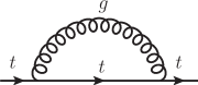
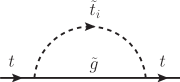
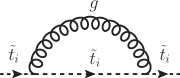
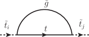
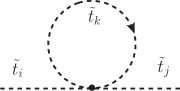
Figure 1: Generic one-loop diagrams for subrenormalization counterterms for the top quark (upper row) and for the scalar tops (lower row) ($i,j,k=1,2$).

2.4 The scalar-top sector of the MSSM

The bilinear part of the top-squark Lagrangian,

$${\cal L}_{\tilde{t},\text{mass}} =-\begin{pmatrix}{{\tilde{t}}_{L}}^{\dagger},{{\tilde{t}}_{R}}^{\dagger}\end{pmatrix}{\mathbf{M}}_{\tilde{t}}\begin{pmatrix}{\tilde{t}}_{L}\\ {\tilde{t}}_{R}\end{pmatrix}\,,$$ (16)

contains the stop-mass matrix

$${\mathbf{M}}_{\tilde{t}} =\begin{pmatrix}M_{\tilde{t}_{L}}^{2}+m_{t}^{2}+M_{Z}^{2}\cos 2\beta\,(T_{t}^{3}-Q_{t}s_{\mathrm{w}}^{2})&m_{t}X_{t}\\[1.99997pt] m_{t}X_{t}&M_{\tilde{t}_{R}}^{2}+m_{t}^{2}+M_{Z}^{2}\cos 2\beta\,Q_{t}\,s_{\mathrm{w}}^{2}\end{pmatrix},$$ (17)

with

$$X_{t} =A_{t}-\mu\,\cot\beta$$ (18)

where $Q_{t}$ and $T_{t}^{3}$ denote the charge and isospin of the top quark, $A_{t}$ the trilinear coupling between the Higgs bosons and the scalar tops, and $\mu$ the Higgsino mass parameter. Below we use $M_{\rm SUSY}:=M_{\tilde{t}_{L}}=M_{\tilde{t}_{R}}$ for our numerical evaluation. The analytical calculation was performed for arbitrary $M_{\tilde{t}_{L}}$ and $M_{\tilde{t}_{R}}$, however. ${\mathbf{M}}_{\tilde{t}}$ can be diagonalized with the help of a unitary transformation matrix ${{\mathbf{U}}}_{\tilde{t}}$, parameterized by a mixing angle ${\theta}_{\tilde{t}}$, to provide the eigenvalues $m_{\tilde{t}_{1}}^{2}$ and $m_{\tilde{t}_{2}}^{2}$ as the squares of the two on-shell top-squark masses.

For the evaluation of the ${\cal O}(\alpha_{t}\alpha_{s})$ two-loop contributions to the self-energies and tadpoles of the Higgs sector, renormalization of the top/stop sector at ${\cal O}(\alpha_{s})$ is required, giving rise to the counterterms for sub-loop renormalization. We follow the renormalization at the one-loop level given in Refs. [23, 56, 57, 58], where details can be found. In particular, in the context of this paper, an OS renormalization is performed for the top-quark mass as well as for the scalar-top masses. This is different from the approach pursued, for example, in Ref. [35], where a $\overline{\mathrm{DR}}$ renormalization was employed, or similarly in the pure $\overline{\mathrm{DR}}$ renormalization presented in Ref. [2]. Using the OS scheme allows us to consistently combine our new correction terms with the hitherto available self-energies included in FeynHiggs.

Besides employing a pure OS renormalization for the top/stop masses in our calculation, we also obtain a result in which the top-quark mass is renormalized $\overline{\mathrm{DR}}$. This new top-quark mass renormalization is included as a new option in the code FeynHiggs. The comparison of the results using the $\overline{\mathrm{DR}}$ and the OS renormalization allows to estimate (some) missing three-loop corrections in the top/stop sector.

Finally, at ${\cal O}(\alpha_{t}\alpha_{s})$, gluinos appear as virtual particles only at the two-loop level (hence, no renormalization for the gluinos is needed). The corresponding soft-breaking gluino mass parameter $M_{3}$ determines the gluino mass, $m_{\tilde{g}}=M_{3}$.

2.5 Evaluation and implementation in the program FeynHiggs

The resulting new contributions to the neutral ${\cal CP}$-even Higgs-boson self-energies, containing all momentum-dependent and additional constant terms, are assigned to the differences

$$\Delta\hat{\Sigma}_{ab}(p^{2})=\hat{\Sigma}_{ab}^{(2)}(p^{2})-\tilde{\Sigma}_{ab}^{(2)}(0)\,,\qquad ab=\{HH,hH,hh\}\,.$$ (19)

These are the new terms evaluated in Ref. [1], included in FeynHiggs. Note the tilde (not hat) on $\tilde{\Sigma}^{(2)}(0)$ which signifies that not only the self-energies are evaluated at zero external momentum but also the corresponding counterterms, following Refs. [20, 21]. A finite shift $\Delta\hat{\Sigma}(0)$ therefore remains in the limit $p^{2}\to 0$ due to $\delta M_{A}^{2(2)}=\mathop{\mathrm{Re}}\Sigma_{AA}^{(2)}(M_{A}^{2})$ being computed at $p^{2}=M_{A}^{2}$ in $\hat{\Sigma}^{(2)}$, but at $p^{2}=0$ in $\tilde{\Sigma}^{(2)}$; for details see Eqs. (13) and (15). For the sake of simplicity we will refer to these terms as ${\cal O}(p^{2}\alpha_{t}\alpha_{s})$ despite the $M_{A}^{2}$ dependence.

3 Discussion of renormalization schemes

In this section we compare our results for the ${\cal O}(p^{2}\alpha_{t}\alpha_{s})$ contributions to the MSSM Higgs-boson self-energies, as given in Ref. [1] to the ones presented subsequently in Ref. [2]. We first show analytically the agreement in the Higgs field renormalization in the two calculations and discuss the differences in the $m_{t}$ renormalizations. We also present some numerical results in both schemes, demonstrating agreement with Ref. [2] once the ${\cal O}(\varepsilon)$ terms are dropped from the top-quark mass counterterm.

Using an OS renormalization for the top-quark mass, the counterterm is determined from the components of the ${\cal O}(\alpha_{s})$ top-quark self-energy (Fig. 1) as follows,

$$\frac{\delta m_{t}^{\rm OS}}{m_{t}} =\frac{1}{2}\mathop{\mathrm{Re}}\left\{\left[\Sigma_{t}^{L}(m_{t}^{2})+\Sigma_{t}^{R}(m_{t}^{2})\right]+\left[\Sigma_{t}^{SL}(m_{t}^{2})+\Sigma_{t}^{SR}(m_{t}^{2})\right]\right\},$$ (20)

where the top-quark self-energy is decomposed according to

$$\Sigma_{t}(p) =\not\!p\,\omega_{-}\Sigma_{t}^{L}(p^{2})+\not\!p\,\omega_{+}\Sigma_{t}^{R}(p^{2})+m_{t}\,\omega_{-}\Sigma_{t}^{SL}(p^{2})+m_{t}\,\omega_{+}\Sigma_{t}^{SR}(p^{2})~{}.$$ (21)

with the projectors $\omega_{\pm}=\frac{1}{2}({\rm 1\mskip-4.25mul}\pm\gamma_{5})$.

3.1 Analytical comparison

In the ${\cal O}(\alpha_{t}\alpha_{s})$ calculation of the Higgs-boson self-energies the renormalization of the top-quark mass at ${\cal O}(\alpha_{s})$ is required. The contributing diagrams are shown in the top row of Fig. 1. The top-quark mass counterterm is inserted into the sub-loop renormalization of the two-loop contributions to the Higgs-boson self-energies, where two sample diagrams are shown in Fig. 2. The left diagram contributes to the momentum-dependent two-loop self-energies, while the right one contributes only to the momentum-independent part. Evaluating the expression in Eq. (20) in $4-2\varepsilon$ dimensions yields the OS top-quark mass counterterm at the one-loop level, which can be written as a Laurent expansion in $\varepsilon$,

$$\delta m_{t}^{\rm OS} =\frac{1}{\varepsilon}\,\delta m_{t}^{\rm div}+\delta m_{t}^{\rm fin}+\varepsilon\,\delta m_{t}^{\varepsilon}+\ldots\,;$$ (22)

higher powers in $\varepsilon$, indicated by the ellipses, do not contribute at the two-loop level for $\varepsilon\to 0$ after renormalization. Accordingly, the $\overline{\mathrm{DR}}$ top-quark mass counterterm is given by the singular part of Eq. (22),

$$\delta m_{t}^{\overline{\mathrm{DR}}} =\frac{1}{\varepsilon}\,\delta m_{t}^{\rm div}\,.$$ (23)

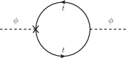
Figure 2: One-loop subrenormalization diagram contributing to $\delta_{\Sigma_{22}}(p^{2})$ and $\delta_{A}(p^{2})$, with the counterterm insertion denoted by a cross. The right diagram only contributes to $\delta_{\Sigma_{22}}(0)$ and $\delta_{A}(0)$.

For further use we define the quantity

$$\delta m_{t}^{\rm FIN} =\frac{1}{\varepsilon}\,\delta m_{t}^{\rm div}+\delta m_{t}^{\rm fin}\,.$$ (24)

At ${\cal O}(\alpha_{s})$ the OS counterterm is given as

$$\frac{\delta m_{t}^{\rm OS}}{m_{t}} =\frac{\alpha_{s}}{6\pi}\,\Bigg{\{}-2\frac{A_{0}(m_{t}^{2})}{m_{t}^{2}}-4\,B_{0}(m_{t}^{2},0,m_{t}^{2})$$

$$\quad-2\frac{A_{0}(m_{\tilde{g}}^{2})}{m_{t}^{2}}+\frac{A_{0}(m_{\tilde{t}_{1}}^{2})}{m_{t}^{2}}+\frac{A_{0}(m_{\tilde{t}_{2}}^{2})}{m_{t}^{2}}$$

$$\quad+\frac{m_{\tilde{g}}^{2}+m_{t}^{2}-m_{\tilde{t}_{1}}^{2}-4\,\sin\theta_{\tilde{t}}\cos\theta_{\tilde{t}}\,m_{\tilde{g}}\,m_{t}}{m_{t}^{2}}\,\mathop{\mathrm{Re}}[B_{0}(m_{t}^{2},m_{\tilde{g}}^{2},m_{\tilde{t}_{1}}^{2})]$$

$$\quad+\frac{m_{\tilde{g}}^{2}+m_{t}^{2}-m_{\tilde{t}_{2}}^{2}+4\,\sin\theta_{\tilde{t}}\cos\theta_{\tilde{t}}\,m_{\tilde{g}}\,m_{t}}{m_{t}^{2}}\,\mathop{\mathrm{Re}}[B_{0}(m_{t}^{2},m_{\tilde{g}}^{2},m_{\tilde{t}_{2}}^{2})]\Bigg{\}}\;.$$ (25)

The one- and two-point functions $A_{0}(m^{2})$ and $B_{0}(p^{2},m_{1}^{2},m_{2}^{2})$ are expanded in $\varepsilon$ as follows,

$$A_{0}(m^{2}) =\frac{1}{\varepsilon}\,A_{0}^{\text{div}}(m^{2})+A_{0}^{\text{fin}}(m^{2})+\varepsilon\,A_{0}^{\varepsilon}(m^{2})~{},$$

$$B_{0}(p^{2},m_{1}^{2},m_{2}^{2}) =\frac{1}{\varepsilon}\,B_{0}^{\text{div}}(p^{2},m_{1}^{2},m_{2}^{2})+B_{0}^{\text{fin}}(p^{2},m_{1}^{2},m_{2}^{2})+\varepsilon\,B_{0}^{\varepsilon}(p^{2},m_{1}^{2},m_{2}^{2})~{}.$$ (26)

Consequently, the term at ${\cal O}(\varepsilon)$, $\delta m_{t}^{\varepsilon}/m_{t}$, is given by Eq. (25), but taking only into account the pieces $\propto A_{0}^{\varepsilon},\,B_{0}^{\varepsilon}$. The special cases of $A_{0}^{\varepsilon}(m^{2})$ and $B_{0}^{\varepsilon}(m^{2},0,m^{2})$ are given by

$$A_{0}^{\varepsilon}(m^{2}) =m^{2}\left\{1-\log(m^{2}/\mu^{2})+\frac{1}{2}\log^{2}(m^{2}/\mu^{2})+\frac{\pi^{2}}{12}\right\},$$

$$B_{0}^{\varepsilon}(m^{2},0,m^{2}) =4-2\,\log(m^{2}/\mu^{2})+\frac{1}{2}\log^{2}(m^{2}/\mu^{2})+\frac{\pi^{2}}{12}\,,$$ (27)

where the factor $4\pi\mathrm{e}^{-\gamma_{E}}$ is absorbed into the renormalization scale. The expression for $B_{0}^{\varepsilon}$ depending on three mass scales can be found e.g. in Ref. [59].

In our calculation in Ref. [1] we include terms up to ${\cal O}(\varepsilon)$, originating from the top-quark self-energy, in the top-mass counterterm, i.e.

$$\delta m_{t}^{\mbox{\tiny\cite[cite]{[\@@bibref{}{Mh-p2-BH4}{}{}]}}}=\delta m_{t}^{\rm OS}~{}.$$ (28)

The derivation in Ref. [2] proceeds differently. The renormalized Higgs-boson self-energies are first calculated in a pure $\overline{\mathrm{DR}}$ scheme. This concerns the top mass, the scalar-top masses, the Higgs field renormalization, and $\tan\beta$. In this way it is ensured that in particular the Higgs fields are renormalized using $\overline{\mathrm{DR}}$, $\delta Z_{{\cal H}_{i}}=\delta Z_{{\cal H}_{i}}^{\overline{\mathrm{DR}}}$, where this quantity contains the contribution from the one- and two-loop level. Using this pure $\overline{\mathrm{DR}}$ scheme a finite result is obtained in which all poles in $1/\varepsilon$ and $1/\varepsilon^{2}$ cancel, such that the limit $\varepsilon\to 0$ can be taken. Subsequently, the $\overline{\mathrm{DR}}$ top-quark mass counterterm, $\delta m_{t}^{\overline{\mathrm{DR}}}$, is replaced by an on-shell counterterm, and the top-quark mass definition is changed accordingly. (The same procedure is applied for the scalar-top masses.) Since these finite expressions for the renormalized Higgs-boson self-energies do not contain any term of ${\cal O}(1/\varepsilon)$, the $\delta m_{t}^{\varepsilon}$ part of the OS top-quark mass counterterm does not contribute, i.e.

$$\delta m_{t}^{\mbox{\tiny\cite[cite]{[\@@bibref{}{Mh-p2-DDVS}{}{}]}}} =\delta m_{t}^{\rm FIN}~{}.$$ (29)

The numerical results for the renormalized Higgs-boson self-energies obtained this way differ significantly from the ones obtained in Ref. [1], as pointed out in Ref. [2].

In the following we discuss the different Higgs-boson field renormalizations, where we use the notation of $\delta Z_{{\cal H}_{2}}^{\delta m_{t}^{\text{X}}}$ for the field renormalization derived using $\delta m_{t}^{\text{X}}$, with $\text{X}=\overline{\mathrm{DR}}$, FIN, $\mathrm{OS}$. The field renormalization can be decomposed into one-loop, two-loop, …parts as

$$\delta Z_{{\cal H}_{2}}^{\delta m_{t}^{\text{X}}} =\delta Z_{{\cal H}_{2}}^{\delta m_{t}^{\text{X}}(1)}+\delta Z_{{\cal H}_{2}}^{\delta m_{t}^{\text{X}}(2)}+\ldots$$ (30)

In Ref. [2] it was claimed that using an OS top-quark mass renormalization from the start results in a non-$\overline{\mathrm{DR}}$ renormalization of $\delta Z_{{\cal H}_{2}}$. While it is correct that an OS value for $m_{t}$ yields different results in the one- and two-loop part,

$$\delta Z_{{\cal H}_{2}}^{\delta m_{t}^{\rm OS}(1)}\neq\delta Z_{{\cal H}_{2}}^{\delta m_{t}^{\overline{\mathrm{DR}}}(1)},\quad\delta Z_{{\cal H}_{2}}^{\delta m_{t}^{\rm OS}(2)}\neq\delta Z_{{\cal H}_{2}}^{\delta m_{t}^{\overline{\mathrm{DR}}}(2)},$$ (31)

the sum of the one- and two-loop parts are identical, independently of the choice of the top-quark mass renormalization (see e.g. Eqs. (3.60)–(3.62) in Ref. [63]),

$$\left(\delta Z_{{\cal H}_{2}}^{\mbox{\tiny\cite[cite]{[\@@bibref{}{Mh-p2-BH4}{}{}]}}}=\right)\;\delta Z_{{\cal H}_{2}}^{\delta m_{t}^{\rm OS}}\Big{|}_{\text{div}} =\delta Z_{{\cal H}_{2}}^{\delta m_{t}^{\rm FIN}}=\delta Z_{{\cal H}_{2}}^{\delta m_{t}^{\overline{\mathrm{DR}}}}\;\left(=\delta Z_{{\cal H}_{2}}^{\mbox{\tiny\cite[cite]{[\@@bibref{}{Mh-p2-DDVS}{}{}]}}}\right)\,,$$ (32)

provided that also in $\delta Z_{{\cal H}_{2}}^{\delta m_{t}^{\rm OS}}$ all finite pieces are dropped, as done in Ref. [1]. Differences between $\delta Z_{{\cal H}_{2}}^{\mbox{\tiny\cite[cite]{[\@@bibref{}{Mh-p2-BH4}{}{}]}}}$ and $\delta Z_{{\cal H}_{2}}^{\mbox{\tiny\cite[cite]{[\@@bibref{}{Mh-p2-DDVS}{}{}]}}}$ arise only at the three-loop level. Consequently, the claim in Ref. [2] that using $\delta m_{t}^{\rm OS}$ leads to an inconsistency in the Higgs field renormalization in Ref. [1] is not correct. The field renormalizations thus cannot be responsible for the observed differences between Refs. [1] and [2].

More explicitly, the difference between the two calculations results from non-vanishing $\delta m_{t}^{\varepsilon}$ terms in the renormalized Higgs-boson self-energies. Those terms naturally appear when performing a full expansion in the dimensional regulator $\varepsilon$. The latter corresponds to choosing $\delta m_{t}^{\rm OS}$ (as done in Ref. [1]) instead of $\delta m_{t}^{\rm FIN}$ (as done in Ref. [2]).

In order to isolate the contributions coming from ${\cal O}(\varepsilon)$ terms $\times$ $1/\varepsilon$ poles we define the following quantities, where superscripts $\mathrm{OS}$, $\mathrm{FIN}$ refer to the respective use of $\delta m_{t}^{\rm OS}$, $\delta m_{t}^{\rm FIN}$:

$$\delta T_{i}^{(2)\mathrm{OS}} =\delta T_{i}^{(2)\,\mathrm{FIN}}+\delta_{T_{i}}~{},$$ (33a)

$$\Sigma_{\phi_{ij}}^{(2)\mathrm{OS}}(p^{2}) =\Sigma_{\phi_{ij}}^{(2)\,\mathrm{FIN}}(p^{2})+\delta_{\Sigma_{ij}}(p^{2})~{},$$ (33b)

$$\Sigma_{AA}^{(2)\mathrm{OS}}(p^{2}) =\Sigma_{AA}^{(2)\,\mathrm{FIN}}(p^{2})+\delta_{A}(p^{2})~{},$$ (33c)

where the last equation yields a shift for the $A$-boson mass counterterm in Eq. (11),

$$\delta M_{A}^{2(2)\mathrm{OS}} =\delta M_{A}^{2(2)\,\mathrm{FIN}}+\delta_{A}(M_{A}^{2})\,.$$ (34)

The $\delta$-terms are defined as the finite contributions stemming from $\delta m_{t}^{\varepsilon}$-dependent parts in the counterterms (see the left diagram in Fig. 2 for an example). The $\overline{\mathrm{DR}}$-renormalized quantities do not contain a finite $\delta m_{t}^{\varepsilon}$-dependent part by definition. Furthermore, since $\phi_{1}$ has no coupling to the top quark, there are no terms proportional to $\delta m_{t}^{\varepsilon}$ in $\Sigma_{\phi_{1}}^{(2)}$, $\Sigma_{\phi_{1}\phi_{2}}^{(2)}$, and $\delta T_{1}^{(2)}$, and it is sufficient to consider $\delta_{\Sigma_{22}}$, $\delta_{A}$, and $\delta_{T_{2}}$ only. While $\delta_{T_{2}}$ is $p^{2}$-independent, we find

$$\delta_{\Sigma_{22}}(p^{2}) =\frac{3\alpha_{t}}{2\pi}\,p^{2}\frac{\delta m_{t}^{\varepsilon}}{m_{t}}+\delta_{\Sigma_{22}}(0)\,,$$ (35)

$$\delta_{A}(p^{2}) =\frac{3\alpha_{t}}{2\pi}\,p^{2}\cos^{2}\!\beta\,\frac{\delta m_{t}^{\varepsilon}}{m_{t}}+\delta_{A}(0)\,.$$ (36)

Using Eqs. (7), (15) we find that the following relations hold for the renormalized Higgs-boson self-energies:

$$-\sin^{2}\!\beta\,\delta_{A}(0)-\frac{e}{2M_{W}s_{\mathrm{w}}}\,\cos^{2}\!\beta\sin\beta\,\delta_{T_{2}} \;=\;0~{}\quad(\text{for }\hat{\Sigma}_{\phi_{1}}^{(2)})\,,$$

$$\sin\beta\cos\beta\,\delta_{A}(0)+\frac{e}{2M_{W}s_{\mathrm{w}}}\,\cos^{3}\!\beta\,\delta_{T_{2}} \;=\;0~{}\quad(\text{for }\hat{\Sigma}_{\phi_{1}\phi_{2}}^{(2)})\,,$$

$$\delta_{\Sigma_{22}}(0)-\cos^{2}\!\beta\,\delta_{A}(0)+\frac{e}{2M_{W}s_{\mathrm{w}}}\,\sin\beta(1+\cos^{2}\!\beta)\,\delta_{T_{2}} \;=\;0~{}\quad(\text{for }\hat{\Sigma}_{\phi_{2}}^{(2)})\,.$$ (37)

This is in agreement with the observation that in the renormalized Higgs-boson self-energies at zero external momentum at ${\cal O}(\alpha_{t}\alpha_{s})$, the terms containing $\delta m_{t}^{\varepsilon}$ drop out in the final (finite) result. Such a cancellation is to be expected as the same combination of one-loop self-energies that potentially contributes to this finite contribution also appears in the ${\cal O}(1/\varepsilon)$ term, where they must cancel. This argument in principle still holds when the momentum-dependent ${\cal O}(\alpha_{t}\alpha_{s})$ corrections are calculated and all counterterms are evaluated with a full expansion in $\varepsilon$. Since the counterterm $\delta_{A}$ is evaluated at $p^{2}=M_{A}^{2}$, and the Higgs-boson fields are renormalized in the $\overline{\mathrm{DR}}$ scheme, however, one finds, using Eqs. (7), (15) for the three renormalized Higgs-boson self-energies,

$$-\sin^{2}\!\beta\,\left(\delta_{A}(M_{A}^{2})-\delta_{A}(0)\right) =\frac{3\alpha_{t}}{2\pi}\left(-\cos^{2}\beta\,\sin^{2}\beta\,M_{A}^{2}\right)\frac{\delta m_{t}^{\varepsilon}}{m_{t}}~{}\;(\mbox{for~{}}\hat{\Sigma}_{\phi_{1}}^{(2)})\,,$$

$$+\sin\beta\cos\beta\,\left(\delta_{A}(M_{A}^{2})-\delta_{A}(0)\right) =\frac{3\alpha_{t}}{2\pi}\left(+\cos^{3}\beta\,\sin\beta\,M_{A}^{2}\right)\frac{\delta m_{t}^{\varepsilon}}{m_{t}}~{}\;(\mbox{for~{}}\hat{\Sigma}_{\phi_{1}\phi_{2}}^{(2)})\,,$$

$$\left(\delta_{\Sigma_{22}}(p^{2})-\delta_{\Sigma_{22}}(0)\right)-\cos^{2}\!\beta\,\left(\delta_{A}(M_{A}^{2})-\delta_{A}(0)\right) =\frac{3\alpha_{t}}{2\pi}\left(p^{2}-\cos^{4}\beta\,M_{A}^{2}\right)\frac{\delta m_{t}^{\varepsilon}}{m_{t}}~{}\;(\mbox{for~{}}\hat{\Sigma}_{\phi_{2}}^{(2)})\,,$$ (38)

i.e. the $\delta m_{t}^{\varepsilon}$ terms contribute in the newly evaluated ${\cal O}(p^{2}\alpha_{t}\alpha_{s})$ corrections. They are $p^{2}$-independent in $\hat{\Sigma}_{\phi_{1}}^{(2)}$ and $\hat{\Sigma}_{\phi_{1}\phi_{2}}^{(2)}$, while they do depend on $p^{2}$ in $\hat{\Sigma}_{\phi_{2}}^{(2)}$.

The $p^{2}$-dependent terms coming from the expansion of terms like $(-p^{2})^{-\varepsilon}$ multiplying a $1/\varepsilon^{2}$ divergence must certainly cancel after inclusion of the counterterms, because non-local terms cannot appear in a renormalizable theory. However, the cancellation of the $\varepsilon$-dependent terms stemming from the mass renormalization is not necessarily fulfilled once the two-loop amplitude carries full momentum dependence. Similarly, the truncation of the field renormalization to the divergent part cuts away terms involving $\delta m_{t}^{\varepsilon}$, leading to further non-cancellations. The explicit $\overline{\mathrm{DR}}$ renormalization of the Higgs-boson fields drops the corresponding finite contributions, such that no $\delta m_{t}^{\rm fin}$, $\delta m_{t}^{\varepsilon}$ terms are taken into account. The different dependence on the external momentum and the $\overline{\mathrm{DR}}$ prescription for the Higgs field renormalization leads to Eqs. (38).

Equivalent momentum-dependent terms of ${\cal O}(\varepsilon)$ of the scalar-top mass counterterms, evaluated from the diagrams in the lower row of Fig. 1, do not contribute. The diagrams with top-squark counterterm insertions are depicted in Fig. 3. The first diagram is momentum independent. In the second diagram, the corresponding loop integral is a massive scalar three-point function ($C_{0}$) with only scalar particles running in the loop, and thus is UV finite. Consequently, the top-squark mass counterterm insertions of ${\cal O}(\varepsilon)$ do not contribute. In the third diagram the stop mass counterterm can enter via the (dependent) counterterm for $A_{t}$ [21, 57]. This diagram does not possess a momentum-dependent divergence, however, and thus the ${\cal O}(\varepsilon)$ term of the scalar top mass counterterm again does not contribute.

             

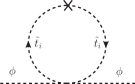
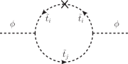
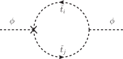
Figure 3: One-loop subrenormalization diagrams containing top-squark loops with counterterm insertions.

3.2 Physics content and interpretation

In the following we give another view on the finite $\delta m_{t}^{\varepsilon}$ term from the top mass renormalization and on the interpretation of the different results for the Higgs-boson masses with and without this term.

In the approximation with $p^{2}=0$ for the two-loop self-energies, the results are the same for either dropping or including the $\delta m_{t}^{\varepsilon}$ term, provided that this is done everywhere in the contributions from the top–stop sector in the renormalized two-loop self-energies.

As explained above, abandoning the $p^{2}=0$ approximation yields an additional $\delta m_{t}^{\varepsilon}$ in the $p^{2}$-coefficient of the self-energy $\Sigma_{\phi_{2}}^{(2)}(p^{2})$ when the on-shell top-quark mass counterterm, see Eq. (22), is used, as well as in the $A$-boson self-energy $\Sigma_{AA}(p^{2})$ from which it induces an additive term $\sim M_{A}^{2}\,\delta m_{t}^{\varepsilon}/m_{t}$ to the mass counterterm $\delta M_{A}^{2}$.

In the renormalized self-energy $\hat{\Sigma}_{\phi_{2}}^{(2)}(p^{2})$, Eq. (7c), this extra $p^{2}$-dependent term survives when $\delta Z_{{\cal H}_{2}}^{(2)}$ is defined in the minimal way containing only the $1/\varepsilon$ and $1/\varepsilon^{2}$ singular parts; however, it disappears in $\hat{\Sigma}_{\phi_{2}}^{(2)}(p^{2})$ when the minimal $\delta Z_{{\cal H}_{2}}^{(2)}=\delta Z_{{\cal H}_{2}}^{\delta m_{t}^{\rm OS}\,(2)}\Big{|}_{\rm div}$ is replaced by

$$\delta Z_{{\cal H}_{2}}^{(2)}\,\to\;\delta Z_{{\cal H}_{2}}^{(2)}-\frac{3\alpha_{t}}{2\pi}\frac{\delta m_{t}^{\varepsilon}}{m_{t}}\,,$$ (39)

which now accommodates also a finite part of two-loop order.

This shift in $\delta Z_{{\cal H}_{2}}^{(2)}$ by a finite term has also an impact on the counterterm for $\tan\beta$ via $\delta\!\tan\beta=\frac{1}{2}\delta Z_{{\cal H}_{2}}^{(2)}$. This has the consequence that the extra $\delta m_{t}^{\varepsilon}$ term in $\delta M_{A}^{2}$ drops out in the constant counterterms for the renormalized self-energies $\hat{\Sigma}_{\phi_{ij}}^{(2)}(p^{2})$ in Eq. (7) because of cancellations with the $\delta m_{t}^{\varepsilon}$ term in $\delta\!\tan\beta$ and $\delta Z_{{\cal H}_{2}}^{(2)}$ (this can be seen from the explicit expressions given in Eqs. (10) and (15) ).

Accordingly, keeping or dropping the finite $\delta m_{t}^{\varepsilon}$ part is thus equivalent to a finite shift in the field-renormalization constant $\delta Z_{{\cal H}_{2}}$ at the two-loop level, which corresponds to a finite shift in $\tan\beta$ as input quantity. Numerically, the shift in $\tan\beta$ is small, and cannot explain the differences in the $M_{h}$ predictions from the two schemes. Hence, these differences originate from the different $p^{2}$ coefficients in $\hat{\Sigma}_{\phi_{2}}^{(2)}(p^{2})$.

The impact of a modification of the two-loop field-renormalization constant on the mass $M_{h}$ can best be studied in terms of the self-energy $\Sigma_{hh}$ in the $h,H$ basis, which is composed of the $\Sigma_{\phi_{ij}}$ in the following way,

$$\Sigma_{hh} =\,\cos^{2}\!\alpha\,\Sigma_{\phi_{2}}+\sin^{2}\!\alpha\,\Sigma_{\phi_{1}}-2\sin\!\alpha\cos\!\alpha\,\Sigma_{\phi_{1}\phi_{2}}\,,$$ (40)

where only $\Sigma_{\phi_{2}}$ contains the $p^{2}$-dependent $\delta m_{t}^{\varepsilon}$ contribution. In order to simplify the discussion and to point to the main features, we assume sufficiently large values of $\tan\beta$ that we can write $\hat{\Sigma}_{hh}\simeq\,\hat{\Sigma}_{\phi_{2}}$, and $h,H$ mixing effects play only a marginal role (both simplifications apply to the numerical discussions in the subsequent section). Moreover, to simplify the notation, we drop the indices and define

$$\Sigma_{hh}\equiv\Sigma,\quad\hat{\Sigma}_{hh}\equiv\hat{\Sigma},\quad\delta Z_{hh}\equiv\delta Z\,,$$ (41)

where $\delta Z_{hh}=\cos^{2}\!\alpha\,\delta Z_{{\cal H}_{2}}+\sin^{2}\!\alpha\,\delta Z_{{\cal H}_{1}}\simeq\delta Z_{{\cal H}_{2}}$. Starting from the tree-level mass $m_{h}$ and the renormalized $h$ self-energy up to the two-loop level,

$$\hat{\Sigma}(p^{2}) =\,\Sigma(p^{2})-\delta m_{h}^{2}+\delta Z(p^{2}-m_{h}^{2})\,,$$ (42)

we obtain the higher-order corrected mass $M_{h}$ from the pole of the propagator, i.e.

$$M_{h}^{2}-m_{h}^{2}+\hat{\Sigma}(M_{h}^{2}) =\,0\,.$$ (43)

The Taylor-expansion of the unrenormalized self-energy around $p^{2}=0$,

$$\Sigma(p^{2}) =\,\Sigma(0)+p^{2}\,\Sigma^{\prime}(0)+\tilde{\Sigma}(p^{2})\,,$$ (44)

yields the first two terms containing the singularities in $1/\varepsilon$ and $1/\varepsilon^{2}$, and the residual fully finite and scheme-independent part denoted by $\tilde{\Sigma}(p^{2})$. With this expansion inserted into Eq. (42) one obtains from the pole condition Eq. (43) the relation

$$(M_{h}^{2}-m_{h}^{2})\big{[}1+\delta Z+\Sigma^{\prime}(0)\big{]}+\big{[}\Sigma(0)-\delta m_{h}^{2}+m_{h}^{2}\,\Sigma^{\prime}(0)\big{]}+\,\tilde{\Sigma}(M_{h}^{2}) =\,0\,,$$ (45)

where the expressions in the square brackets are each finite, irrespective of a possible finite term in the definition of $\delta Z$.

Taking into account that $M_{h}^{2}$ differs from $m_{h}^{2}$ by a a higher-order shift, we can replace

$$\tilde{\Sigma}(M_{h}^{2}) =\,\tilde{\Sigma}(m_{h}^{2})+(M_{h}^{2}-m_{h}^{2})\,\tilde{\Sigma}^{\prime}(m_{h}^{2})+\cdots$$ (46)

and obtain

$$M_{h}^{2}-m_{h}^{2} =\,-\frac{\Sigma(0)-\delta m_{h}^{2}+m_{h}^{2}\,\Sigma^{\prime}(0)+\tilde{\Sigma}(m_{h}^{2})}{1+\delta Z+\Sigma^{\prime}(0)+\tilde{\Sigma}^{\prime}(m_{h}^{2})}$$ (47)

$$=\,-\big{[}\Sigma(0)-\delta m_{h}^{2}+m_{h}^{2}\,\Sigma^{\prime}(0)+\tilde{\Sigma}(m_{h}^{2})\big{]}_{\rm 1loop\,+\,2loop}$$

$$\quad+\big{[}\Sigma(0)-\delta m_{h}^{2}+m_{h}^{2}\,\Sigma^{\prime}(0)+\tilde{\Sigma}(m_{h}^{2})\big{]}_{\rm 1loop}\cdot\big{[}\delta Z+\Sigma^{\prime}(0)+\tilde{\Sigma}^{\prime}(m_{h}^{2})\big{]}_{\rm 1loop}+\,\cdots$$

showing explicitly all terms up to two-loop order. It does not contain the two-loop part of the field-renormalization constant, which indeed would show up at the three-loop level. Hence, effects resulting from different conventions for $\delta Z^{({\rm 2loop})}$ in the finite part have to be considered in the current situation as part of the theoretical uncertainty.

3.3 Numerical comparison

In this section the renormalized momentum-dependent ${\cal O}(p^{2}\alpha_{t}\alpha_{s})$ self-energy contributions $\Delta\hat{\Sigma}_{hh}$, $\Delta\hat{\Sigma}_{hH}$, $\Delta\hat{\Sigma}_{HH}$ of Eq. (19) and the mass shifts

$$\Delta M_{h}=M_{h}-M_{h,0},\quad\Delta M_{H}=M_{H}-M_{H,0}$$ (48)

are compared using either $\delta m_{t}^{\rm OS}$ or $\delta m_{t}^{\rm FIN}$, as discussed above. $M_{h,0}$ and $M_{H,0}$ denote the Higgs-boson mass predictions without the newly obtained ${\cal O}(p^{2}\alpha_{t}\alpha_{s})$ corrections.

The results are obtained for two different scenarios. Scenario 1 is adopted from the $m_{h}^{\rm max}$ scenario described in Ref. [64]. We use the following parameters:

$$m_{t} =173.2\,\,\mathrm{GeV},\;M_{\rm SUSY}=1\,\,\mathrm{TeV},\;X_{t}=2\,M_{\rm SUSY}\;,$$

$$m_{\tilde{g}} =1500\,\,\mathrm{GeV},\;\mu=M_{2}=200\,\,\mathrm{GeV}\,.$$ (49)

Here $M_{2}$ denotes the $SU(2)$ soft SUSY-breaking parameter, where the $U(1)$ parameter is derived via the GUT relation $M_{1}=(5/3)\,(s_{\mathrm{w}}^{2}/c_{\mathrm{w}}^{2})\,M_{2}$. Scenario 2 is an updated version of the “light-stop scenario” of Refs. [64, 65]

$$m_{t} =173.2\,\,\mathrm{GeV},\;M_{\rm SUSY}=0.5\,\,\mathrm{TeV},\;X_{t}=2\,M_{\rm SUSY}\;,$$

$$m_{\tilde{g}} =1500\,\,\mathrm{GeV},\;\mu=M_{2}=400\,\,\mathrm{GeV}\;M_{1}=340\,\,\mathrm{GeV}\,,$$ (50)

leading to stop mass values of

$$m_{\tilde{t}_{1}}=326.8\,\,\mathrm{GeV},\;m_{\tilde{t}_{2}}=673.2\,\,\mathrm{GeV}~{}.$$ (51)

A renormalization scale of $\mu=m_{t}$ is set in all numerical evaluations.

Self-energies

In Fig. 4 we present the results for the $\delta_{A}$ (upper plot) and $\delta_{\Sigma_{22}}$ (lower plot) contributions for $\tan\beta=5(20)$ in red (blue) in Scenario 1, where $\delta_{A},\delta_{\Sigma_{22}}$ are defined in Eqs. (33). In the upper plot $\delta_{A}(M_{A}^{2})$ ($\delta_{A}(0)$) is shown as solid (dashed) line; correspondingly, in the lower plot $\delta_{\Sigma_{22}}(p^{2})$ ($\delta_{\Sigma_{22}}(0)$) is depicted as solid (dashed) line. The contribution is seen to decrease quadratically with $M_{A}$ or $p\ (:=\sqrt{p^{2}})$ when including the momentum-dependent terms, see Eq. (38). For $\delta_{A}$ it is suppressed with $\tan^{2}\beta$. For high values of $M_{A}$ and low $\tan\beta$, the $\delta_{A}$ contribution becomes sizable. Similarly, for large $p$ the $\delta_{\Sigma_{22}}$ term becomes sizable, showing the relevance of the $\delta m_{t}^{\varepsilon}$ contribution.

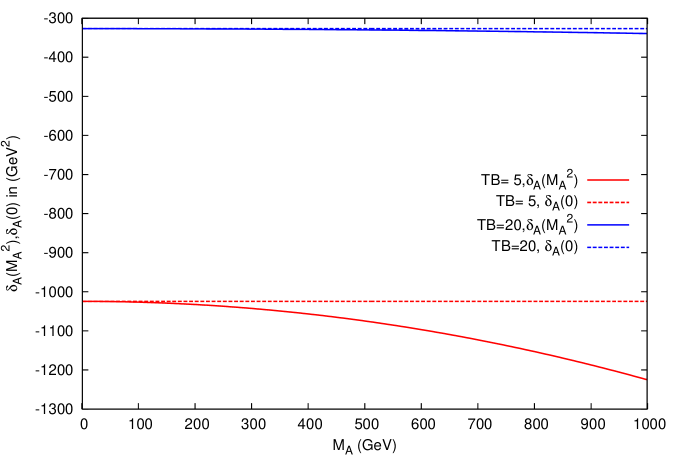
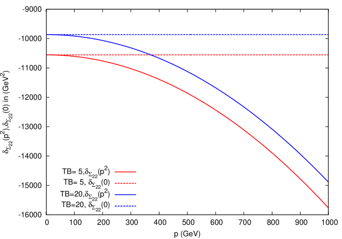
Figure 4: $\delta_{A}(M_{A}^{2})$ and $\delta_{A}(0)$ varying $M_{A}$ shown in the upper plot, $\delta_{\Sigma_{22}}(p^{2})$ and $\delta_{\Sigma_{22}}(0)$ in the lower plot, both within Scenario 1.

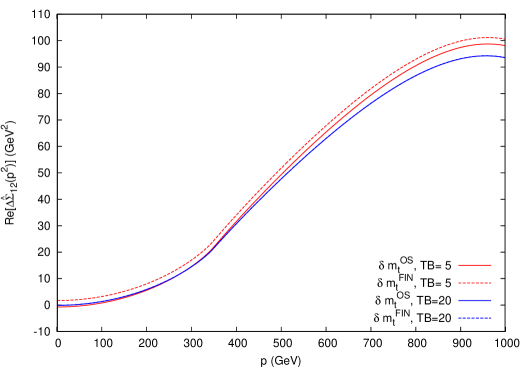
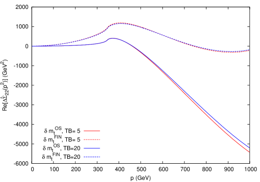
Figure 5: $\Delta\hat{\Sigma}_{\phi_{ij}}$ in Scenario 1 (with $M_{A}=250\,\,\mathrm{GeV}$) for $ij=11,12,22$ in the upper, the middle and the lower plot, respectively. The solid (dashed) lines show the result obtained with $\delta m_{t}^{\rm OS}$ ($\delta m_{t}^{\rm FIN}$); the red (blue) lines correspond to $\tan\beta=5(20)$.

The behavior of the real parts of the two-loop contributions to the self-energies $\Delta\hat{\Sigma}_{ab}$ is analyzed in Fig. 5. Solid lines show the result evaluated with $\delta m_{t}^{\rm OS}$, as obtained in Ref. [1] (i.e. the new contribution added to the previous FeynHiggs result in Ref. [1], see Eq. (19)). Dashed lines show the result evaluated with $\delta m_{t}^{\rm FIN}$, as obtained in Ref. [2]. We show $M_{A}=250\,\,\mathrm{GeV}$ and $\tan\beta=5(20)$ as red (blue) lines. The difference between the $\delta m_{t}^{\rm FIN}$ and $\delta m_{t}^{\rm OS}$ calculations for $\Delta\hat{\Sigma}_{\phi_{1}}$ and $\Delta\hat{\Sigma}_{\phi_{1}\phi_{2}}$ is $p$-independent, as discussed below Eq. (38), and the difference between the two schemes is numerically small. For $\Delta\hat{\Sigma}_{\phi_{2}}$, on the other hand, the difference becomes large for large values of $p$. This self-energy contribution is mostly relevant for the light ${\cal CP}$-even Higgs-boson, however, i.e. for $p\sim M_{h}$, and thus the relevant numerical difference remains relatively small (but non-zero) compared to the larger differences at large $p$. For completeness it should be mentioned that the imaginary part is not affected by the variation of the top-quark renormalization, as only the real parts of the counterterm insertions enter the calculation.

Scenario 2 was omitted as the relevant aspects for the analysis of the self-energies using $\delta m_{t}^{\rm OS}$ vs. $\delta m_{t}^{\rm FIN}$ have become sufficiently apparent within Scenario 1.

Mass shifts

We now turn to the effects on the neutral ${\cal CP}$-even Higgs-boson masses themselves. The numerical effects on the two-loop corrections to the Higgs-boson masses $M_{h,H}$ are investigated by analyzing the mass shifts $\Delta M_{h}$ and $\Delta M_{H}$ of Eq. (48). The results are shown for the two renormalization schemes for the top-quark mass, i.e. using $\delta m_{t}^{\rm OS}$ or $\delta m_{t}^{\rm FIN}$. The color coding is as in Fig. 5. The results for Scenario 1 are shown in Fig. 6 and are in agreement with Figs. 2 and 3 (left) in Ref. [2], i.e. we reproduce the results of Ref. [2] using $\delta m_{t}^{\rm FIN}$. The results for Scenario 2 are shown in Fig. 7. The results are again in agreement with Figs. 2 and 3 (right) in Ref. [2]. This agreement confirms the use of $\delta m_{t}^{\rm FIN}$ in Ref. [2], in comparison with $\delta m_{t}^{\rm OS}$ used in the evaluation of our results. For the contribution to $M_{H}$, peaks can be observed at $M_{A}=2m_{\tilde{t}_{1}}$, $m_{\tilde{t}_{1}}+m_{\tilde{t}_{2}}$, $2m_{\tilde{t}_{2}}$, see also Ref. [1] and the discussion of Fig. 9 below.

Since the the results using $\delta m_{t}^{\rm OS}$ and $\delta m_{t}^{\rm FIN}$ correspond to two different renormalization schemes, their difference should be regarded as an indication of missing higher-order momentum-dependent corrections.

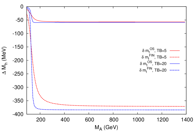
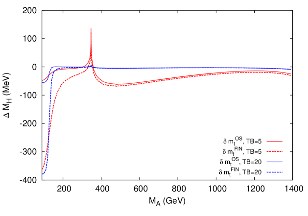
Figure 6: Variation of the mass shifts $\Delta M_{h},\Delta M_{H}$ with the $A$-boson mass $M_{A}$ within Scenario 1, for $\tan\beta=5$ (red) and $\tan\beta=20$ (blue) in- or excluding some $\delta$ terms. The peak in $\Delta M_{H}$ originates from a threshold at $2\,m_{t}$.

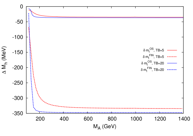
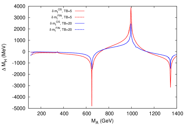
Figure 7: Variation of the mass shifts $\Delta M_{h},\Delta M_{H}$ with the $A$-boson mass $M_{A}$ within Scenario 2, for $\tan\beta=5$ (red) and $\tan\beta=20$ (blue) in- or excluding some $\delta$ terms. The peaks in $\Delta M_{H}$ originate from thresholds at $2\,m_{t}$, $2\,m_{\tilde{t}_{1}}$, $m_{\tilde{t}_{1}}+m_{\tilde{t}_{2}}$ and $2\,m_{\tilde{t}_{2}}$, where the threshold at $2\,m_{t}$ is suppressed by $1/\tan^{2}\beta$.

4 Comparison with the $m_{t}$ $\overline{\mathrm{DR}}$ renormalization

Having examined the renormalization of the top-quark mass, we will now analyze the numerical differences between an $m_{t}^{\overline{\mathrm{DR}}}$ and an $m_{t}^{\mathrm{OS}}$ calculation. This has been realized by employing a $\overline{\mathrm{DR}}$ renormalization of the top-quark mass in all steps of the calculation. The top-squark masses are kept renormalized on-shell. This can be seen as an intermediate step towards a full $\overline{\mathrm{DR}}$ analysis.

4.1 Implementation in the program FeynHiggs

In the $\overline{\mathrm{DR}}$ scheme the top-quark mass parameter entering the calculation is the MSSM $\overline{\mathrm{DR}}$ top-quark mass, which at one-loop order is related to the pole mass $m_{t}$ (given in the user input) in the following way,

$$m_{t}^{\overline{\mathrm{DR}}}(\mu) =m_{t}\cdot\left[1+\frac{\delta m_{t}^{\rm fin}}{m_{t}}+\mathcal{O}\left(\bigl{(}\alpha_{s}^{\overline{\mathrm{DR}}}\bigr{)}^{2}\right)\right]\,.$$ (52)

The term $\delta m_{t}^{\rm fin}$ can be obtained from Eq. (22), with the formal replacement $\alpha_{s}\rightarrow\alpha_{s}^{\overline{\mathrm{DR}}}(\mu)$, yielding

$$\frac{\delta m_{t}^{\rm fin}}{m_{t}}=\alpha_{s}^{\overline{\mathrm{DR}}}(\mu) \left(-\frac{5}{3\pi}+\frac{1}{\pi}\log(m_{t}^{2}/\mu^{2})+\frac{m_{\tilde{g}}^{2}}{3m_{t}^{2}\pi}\left(-1+\log(m_{\tilde{g}}^{2}/\mu^{2})\right)\right.$$

$$+\frac{1}{6m_{t}^{2}\pi}\Bigl{(}m_{\tilde{t}_{1}}^{2}(1-\log(m_{\tilde{t}_{1}}^{2}/\mu^{2}))+m_{\tilde{t}_{2}}^{2}(1-\log(m_{\tilde{t}_{2}}^{2}/\mu^{2}))$$

$$+(m_{\tilde{g}}^{2}+m_{t}^{2}-m_{\tilde{t}_{1}}^{2}-2m_{\tilde{g}}m_{t}\sin(2\theta_{t}))\mathop{\mathrm{Re}}[B_{0}^{\rm fin}(m_{t}^{2},m_{\tilde{g}}^{2},m_{\tilde{t}_{1}}^{2})]$$

$$+(m_{\tilde{g}}^{2}+m_{t}^{2}-m_{\tilde{t}_{2}}^{2}+2m_{\tilde{g}}m_{t}\sin(2\theta_{t}))\mathop{\mathrm{Re}}[B_{0}^{\mathrm{fin}}(m_{t}^{2},m_{\tilde{g}}^{2},m_{\tilde{t}_{2}}^{2})]\Bigr{)}\biggr{)}.$$ (53)

At zeroth order, $\alpha_{s}^{\overline{\mathrm{DR}}}(\mu)=\alpha_{s}^{\overline{\mathrm{MS}}}(\mu)$.

As on-shell renormalized quantities the stop masses $m_{\tilde{t}_{1}}$ and $m_{\tilde{t}_{2}}$ should have fixed values, independently of the renormalization chosen for the top-quark mass. We compensate for the changes induced by $\delta m_{t}^{\rm fin}$ in the stop mass matrix, Eq. (17), by shifting the SUSY-breaking parameters as follows,

$$M_{\tilde{t}_{L}}^{2} \to M_{\tilde{t}_{L}}^{\prime 2}=M_{\tilde{t}_{L}}^{2}+(m_{t}^{\mathrm{OS}})^{2}-(m_{t}^{\overline{\mathrm{DR}}})^{2}\,,$$ (54a)

$$M_{\tilde{t}_{R}}^{2} \to M_{\tilde{t}_{R}}^{\prime 2}=M_{\tilde{t}_{R}}^{2}+(m_{t}^{\mathrm{OS}})^{2}-(m_{t}^{\overline{\mathrm{DR}}})^{2}\,,$$ (54b)

$$A_{t} \to A_{t}^{\prime}=\frac{m_{t}^{\mathrm{OS}}}{m_{t}^{\overline{\mathrm{DR}}}}\left(A_{t}-\frac{\mu}{\tan\beta}\right)+\frac{\mu}{\tan\beta}\,.$$ (54c)

(Except for $A_{t}$, which actually appears in the Feynman rules, FeynHiggs only pretends to perform these shifts but computes the sfermion masses using $m_{t}^{\mathrm{OS}}$.)

This procedure is available in FeynHiggs from version 2.11.1 on and is activated by setting the new value 2 for the runningMT flag. The comparison of the results with $\overline{\mathrm{DR}}$ and with OS renormalization admits an improved estimate of (some) of the missing three-loop corrections in the top/stop sector.

4.2 Numerical analysis

In the following plots we show the difference

$$\bar{\Delta}M_{\phi}:=M_{\phi}(m_{t}^{\mathrm{OS}})-M_{\phi}(m_{t}^{\overline{\mathrm{DR}}}),\quad\phi=h,H,$$ (55)

between $M_{\phi}$ evaluated in the OS scheme, i.e. using $m_{t}^{\mathrm{OS}}$ (not $m_{t}^{\mathrm{FIN}}$), and in the $\overline{\mathrm{DR}}$ scheme, i.e. using $m_{t}^{\overline{\mathrm{DR}}}$.

Dependence on $M_{A}$

In the upper half of Fig. 8, $\bar{\Delta}M_{h}$ is plotted in Scenario 1 as a function of $M_{A}$ with $\tan\beta=5(20)$ in red (blue). The solid (dashed) lines show the difference evaluated at the full one-loop level (including the ${\cal O}(\alpha_{t}\alpha_{s})$ corrections). The dotted lines include the newly calculated ${\cal O}(p^{2}\alpha_{t}\alpha_{s})$ corrections. For $M_{A}\;\raisebox{-3.00003pt}{$\stackrel{{\scriptstyle\displaystyle>}}{{\sim}}$}\;200\,\,\mathrm{GeV}$ one observes large differences of ${\cal O}(10\,\,\mathrm{GeV})$ at the one-loop level, indicating the size of missing higher-order corrections from the top/stop sector beyond one-loop. This difference is strongly reduced at the two-loop level, to about $\sim 3\,\,\mathrm{GeV}$, now corresponding to missing higher orders beyond two-loop from the top/stop sector. The dotted lines are barely visible below the dashed lines, indicating the relatively small effect of the ${\cal O}(p^{2}\alpha_{t}\alpha_{s})$ corrections as derived in Ref. [1].

The lower plot of Fig. 8 shows the corresponding results for $\bar{\Delta}M_{H}$ with the same color/line coding. Here large effects are only visible for low $M_{A}$, where the higher-order corrections to $M_{H}$ are sizable (and the light Higgs-boson receives only very small higher-order corrections). In this part of the parameter space the same reduction of $\bar{\Delta}M_{H}$ going from one-loop to two-loop can be observed.

The behavior is similar for Scenario 2, shown in Fig. 9 (with the same line/color coding as in Fig. 8), only the size of the difference $\bar{\Delta}M_{h}$ is $\sim 20\%$ smaller at the one-loop, and $\sim 50\%$ smaller at the two-loop level compared to Scenario 1. The same peak structure due to thresholds as in Fig. 7 is visible.

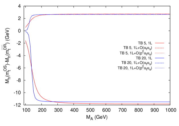
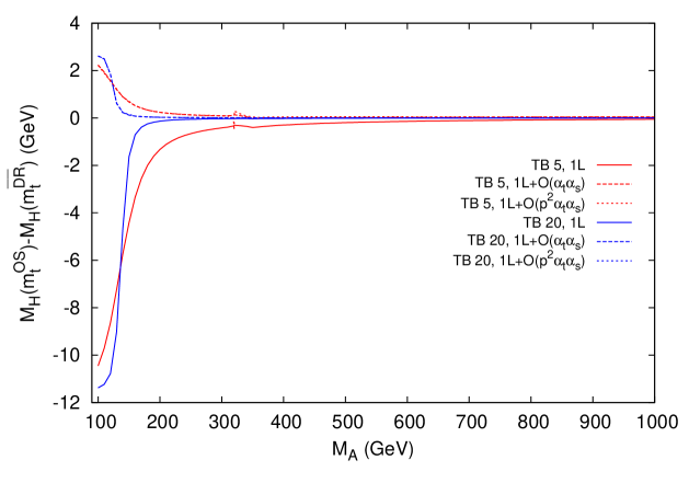
Figure 8: $\bar{\Delta}M_{\phi}=M_{\phi}(m_{t}^{\mathrm{OS}})-M_{\phi}(m_{t}^{\overline{\mathrm{DR}}})$ for $\phi=h$ (upper plot) and $\phi=H$ (lower plot). The difference is shown as solid (dashed/dotted) line at the one-loop (${\cal O}(\alpha_{t}\alpha_{s})$/${\cal O}(p^{2}\alpha_{t}\alpha_{s})$) level as a function of $M_{A}$ for $\tan\beta=5(20)$ in red (blue) within Scenario 1.

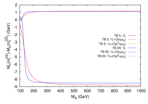
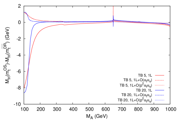
Figure 9: $\bar{\Delta}M_{\phi}=M_{\phi}(m_{t}^{\mathrm{OS}})-M_{\phi}(m_{t}^{\overline{\mathrm{DR}}})$ for $\phi=h$ (upper plot) and $\phi=H$ (lower plot) as a function of $M_{A}$ within Scenario 2, with the same line/color coding as in Fig. 8. The peak in the lower plot originates from a threshold at $2\,m_{\tilde{t}_{1}}$. The threshold at $2\,m_{t}$ is suppressed by $1/\tan^{2}\beta$.

Dependence on $m_{\tilde{g}}$

In Figs. 10, 11 we analyze $\bar{\Delta}M_{\phi}$ as a function of $m_{\tilde{g}}$ in Scenario 1 and 2, respectively. We fix $M_{A}=250\,\,\mathrm{GeV}$ and use the same line/color coding as in Fig. 8. Due to the choice of an MSSM $\overline{\mathrm{DR}}$ top-quark mass definition, $m_{t}^{\overline{\mathrm{DR}}}$ varies with $m_{\tilde{g}}$ already at the one-loop level.

In the upper plots we show the light ${\cal CP}$-even Higgs-boson case, where it can be observed that the scheme dependence is strongly reduced at the two-loop level. It reaches $2-3\,\,\mathrm{GeV}$ in Scenario 1 and $\sim 1\,\,\mathrm{GeV}$ in Scenario 2, largely independently of $\tan\beta$. At the one-loop level the scheme dependence grows with $m_{\tilde{g}}$, whereas the dependence is much milder at the two-loop level. The effects of the ${\cal O}(p^{2}\alpha_{t}\alpha_{s})$ corrections become visible at larger $m_{\tilde{g}}$, in agreement with Ref. [1].

The heavy ${\cal CP}$-even Higgs-boson case is shown in the lower plots. At small $\tan\beta$ scheme differences of ${\cal O}(600\,\,\mathrm{MeV}(150\,\,\mathrm{MeV}))$ can be observed at the one-(two-)loop level. For large $\tan\beta$ the differences always stay below ${\cal O}(50\,\,\mathrm{MeV})$, in agreement with Fig. 8. The dependence on $m_{\tilde{g}}$ is similar as for the light Higgs-boson, but again somewhat weaker.

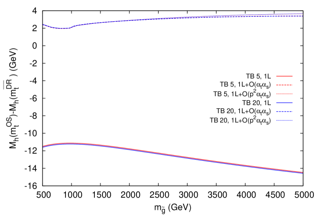
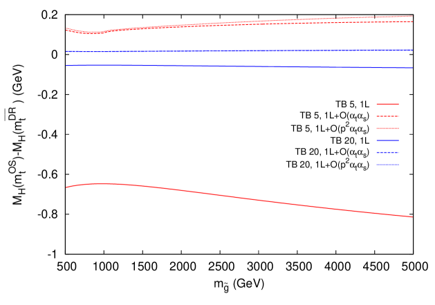
Figure 10: $\bar{\Delta}M_{\phi}=M_{\phi}(m_{t}^{\mathrm{OS}})-M_{\phi}(m_{t}^{\overline{\mathrm{DR}}})$ for $\phi=h$ (upper plot) and $\phi=H$ (lower plot) as a function of $m_{\tilde{g}}$ within Scenario 1, for $M_{A}=250\,\,\mathrm{GeV}$ and with the same line/color coding as in Fig. 8.

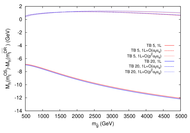
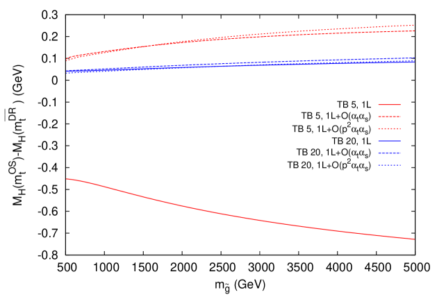
Figure 11: $\bar{\Delta}M_{\phi}=M_{\phi}(m_{t}^{\mathrm{OS}})-M_{\phi}(m_{t}^{\overline{\mathrm{DR}}})$ for $\phi=h$ (upper plot) and $\phi=H$ (lower plot) as a function of $m_{\tilde{g}}$ within Scenario 2, for $M_{A}=250\,\,\mathrm{GeV}$ and with the same line/color coding as in Fig. 8.

Dependence on $X_{t}$

Finally, in Figs. 12, 13 we analyze $\bar{\Delta}M_{\phi}$ as a function of $X_{t}=X_{t}^{\mathrm{OS}}$ in Scenario 1 and 2, respectively. We again fix $M_{A}=250\,\,\mathrm{GeV}$ and use the same line/color coding as in Fig. 8.

In the upper plots we show the light ${\cal CP}$-even Higgs-boson case. As before the scheme dependence is strongly reduced when going from the one-loop to the two-loop case. In general a smaller scheme dependence is found from small $X_{t}$, while it increases for larger $|X_{t}|$ values, in agreement with Ref. [66]. For most parts of the parameter space, when the two-loop corrections are included, it is found to be below $\sim 3\,\,\mathrm{GeV}$. The contribution of ${\cal O}(p^{2}\alpha_{t}\alpha_{s})$ remains small for all $X_{t}$ values.

In the heavy ${\cal CP}$-even Higgs-boson case, shown in the lower plots, the dependence of the size of the effects is slightly more involved, though the general picture of a strongly reduced scheme dependence can be observed here, too. In both scenarios, for large negative $X_{t}$ and $\tan\beta=5$ the ${\cal O}(p^{2}\alpha_{t}\alpha_{s})$ contributions can become sizable with respect to the ${\cal O}(\alpha_{t}\alpha_{s})$ corrections.

In conclusion, the scheme dependence is found to be reduced substantially when going from the pure one-loop calculation to the two-loop ${\cal O}(\alpha_{t}\alpha_{s})$ corrections. This indicates that corrections at the three-loop level and beyond, stemming from the top/stop sector are expected at the order of the observed scheme dependence, i.e. at the level of $\sim 3\,\,\mathrm{GeV}$. This is in agreement with existing calculations beyond two-loop [40, 37]. A further reduction of the scheme dependence might be expected by adding the ${\cal O}(\alpha_{t}^{2})$ contributions. The $m_{t}^{\overline{\mathrm{DR}}}$ value calculated at ${\cal O}(\alpha_{s}+\alpha_{t})$ is substantially closer to $m_{t}^{\mathrm{OS}}$, reducing already strongly the scheme dependence at the one-loop level. This extended analysis is beyond the scope of our paper, however.

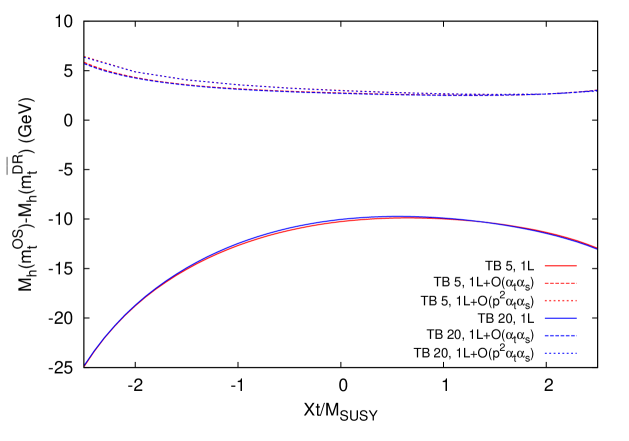
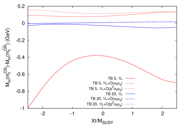
Figure 12: $\bar{\Delta}M_{\phi}=M_{\phi}(m_{t}^{\mathrm{OS}})-M_{\phi}(m_{t}^{\overline{\mathrm{DR}}})$ for $\phi=h$ (upper plot) and $\phi=H$ (lower plot) as a function of $X_{t}=X_{t}^{\mathrm{OS}}$ within Scenario 1, with the same line/color coding as in Fig. 8.

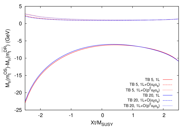
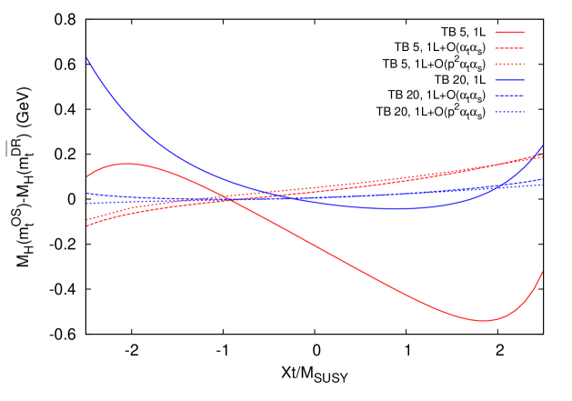
Figure 13: $\bar{\Delta}M_{\phi}=M_{\phi}(m_{t}^{\mathrm{OS}})-M_{\phi}(m_{t}^{\overline{\mathrm{DR}}})$ for $\phi=h$ (upper plot) and $\phi=H$ (lower plot) as a function of $X_{t}=X_{t}^{\mathrm{OS}}$ within Scenario 2, with the same line/color coding as in Fig. 8.

5 Conclusions

In this paper we analyzed the scheme dependence of the ${\cal O}(\alpha_{t}\alpha_{s})$ corrections to the neutral ${\cal CP}$-even Higgs-boson masses in the MSSM. In a first step we investigated the differences in the ${\cal O}(p^{2}\alpha_{t}\alpha_{s})$ corrections as obtained in Refs. [1] and [2]. We have shown that the difference can be attributed to different renormalizations of the top-quark mass. In both calculations an “on-shell” top-quark mass was employed. The evaluation in Ref. [1] includes the ${\cal O}(\varepsilon)$ terms of the top-quark mass counterterm, $\delta m_{t}^{\varepsilon}$, however, whereas this contribution was omitted in Ref. [2]. We have shown analytically that the terms involving $\delta m_{t}^{\varepsilon}$ do not cancel in the ${\cal O}(p^{2}\alpha_{t}\alpha_{s})$ corrections to the renormalized Higgs-boson self-energies (an effect that was already observed in the ${\cal O}(\alpha_{t}\alpha_{s})$ corrections in the NMSSM Higgs sector [63]). Numerical agreement between Refs. [1] and [2] is found as soon as the $\delta m_{t}^{\varepsilon}$ terms are dropped from the calculation in Ref. [1]. Moreover, as an alternative interpretation, we have shown that omitting the $\delta m_{t}^{\varepsilon}$ terms is equivalent to a redefinition of the finite part of the two-loop field-renormalization constant which affects the Higgs-boson mass prediction at the three-loop order (apart from a numerically insignificant shift in $\tan\beta$ as an input parameter). The differences between the two calculations can thus be regarded as an indication of the size of the missing momentum-dependent corrections beyond the two-loop level, and reach up to several hundred MeV in the case of the light ${\cal CP}$-even Higgs-boson.

In a second step we performed a calculation of the ${\cal O}(\alpha_{t}\alpha_{s})$ and ${\cal O}(p^{2}\alpha_{t}\alpha_{s})$ corrections employing a $\overline{\mathrm{DR}}$ top-quark mass counterterm. We analyzed the numerical difference of the Higgs-boson masses evaluated with $\delta m_{t}^{\rm OS}$ and with $\delta m_{t}^{\overline{\mathrm{DR}}}$. By varying the ${\cal CP}$-odd Higgs-boson mass, $M_{A}$, the gluino mass, $m_{\tilde{g}}$ and the off-diagonal entry in the scalar-top mass matrix, $X_{t}$, we found that in all cases the scheme dependence, in particular of the light ${\cal CP}$-even Higgs-boson mass, is strongly reduced by going from the full one-loop result to the two-loop result including the ${\cal O}(\alpha_{t}\alpha_{s})$ corrections. The further inclusion of the ${\cal O}(p^{2}\alpha_{t}\alpha_{s})$ contributions had a numerically small effect. The differences found at the two-loop level indicate that corrections at the three-loop level and beyond, stemming from the top/stop sector, are expected at the level of $\sim 3\,\,\mathrm{GeV}$. This is in agreement with existing calculations beyond two-loop [40, 37]. The possibility to use $m_{t}^{\overline{\mathrm{DR}}}$ instead of $m_{t}^{\mathrm{OS}}$ has been added to the FeynHiggs package and allows an improved estimate of the size of missing corrections beyond the two-loop order.

Acknowledgements

We thank P. Breitenlohner, H. Haber, S. Jones, M. Mühlleitner, H. Rzehak, P. Slavich and G. Weiglein, for helpful discussions. The work of S.H. is supported in part by CICYT (grant FPA 2013-40715-P) and by the Spanish MICINN’s Consolider-Ingenio 2010 Program under Grant MultiDark No. CSD2009-00064. S.B. gratefully acknowledges financial support by the ERC Advanced Grant MC@NNLO (340983). This research was supported in part by the Research Executive Agency (REA) of the European Union under the Grant Agreement PITN-GA2012-316704 (HiggsTools).

References

- [1] S. Borowka, T. Hahn, S. Heinemeyer, G. Heinrich and W. Hollik, Eur. Phys. J. C 74 (2014) 8, 2994 [arXiv:1404.7074 [hep-ph]].
- [2] G. Degrassi, S. Di Vita and P. Slavich, Eur. Phys. J. C 75 (2015) 2, 61 [arXiv:1410.3432 [hep-ph]].
- [3] G. Aad et al. [ATLAS Collaboration], Phys. Lett. B 716 (2012) 1 [arXiv:1207.7214 [hep-ex]].
- [4] S. Chatrchyan et al. [CMS Collaboration], Phys. Lett. B 716 (2012) 30 [arXiv:1207.7235 [hep-ex]].
- [5] G. Aad et al. [ATLAS and CMS Collaborations], arXiv:1503.07589 [hep-ex].
- [6] The ATLAS collaboration, ATLAS-CONF-2015-008, ATLAS-COM-CONF-2015-006.
- [7] V. Khachatryan et al. [CMS Collaboration], arXiv:1412.8662 [hep-ex].
-
[8]
H. Nilles,
Phys. Rept. 110 (1984) 1;
H. Haber and G. Kane, Phys. Rept. 117 (1985) 75;
R. Barbieri, Riv. Nuovo Cim. 11 (1988) 1. -
[9]
A. Djouadi,
Phys. Rept. 459 (2008) 1
[arXiv:hep-ph/0503173];
S. Heinemeyer, Int. J. Mod. Phys. A 21 (2006) 2659 [arXiv:hep-ph/0407244]. - [10] S. Heinemeyer, W. Hollik and G. Weiglein, Phys. Rept. 425 (2006) 265 [arXiv:hep-ph/0412214].
- [11] M. Frank, T. Hahn, S. Heinemeyer, W. Hollik, H. Rzehak and G. Weiglein, JHEP 0702 (2007) 047 [arXiv:hep-ph/0611326].
- [12] S. Heinemeyer, W. Hollik, H. Rzehak and G. Weiglein, Phys. Lett. B 652 (2007) 300 [arXiv:0705.0746 [hep-ph]].
- [13] D. Demir, Phys.Rev. D 60 (1999) 055006 [arXiv:hep-ph/9901389].
- [14] A. Pilaftsis and C. Wagner, Nucl. Phys. B 553 (1999) 3 [arXiv:hep-ph/9902371].
- [15] W. Hollik and S. Paßehr, JHEP 1410 (2014) 171 [arXiv:1409.1687[hep-ph]].
-
[16]
J. Ellis, G. Ridolfi and F. Zwirner,
Phys. Lett. B 257 (1991) 83;
Y. Okada, M. Yamaguchi and T. Yanagida, Prog. Theor. Phys. 85 (1991) 1;
H. Haber and R. Hempfling, Phys. Rev. Lett. 66 (1991) 1815. - [17] A. Brignole, Phys. Lett. B 281 (1992) 284.
- [18] P. Chankowski, S. Pokorski and J. Rosiek, Phys. Lett. B 286 (1992) 307; Nucl. Phys. B 423 (1994) 437 [arXiv:hep-ph/9303309].
- [19] A. Dabelstein, Nucl. Phys. B 456 (1995) 25 [arXiv:hep-ph/9503443]; Z. Phys. C 67 (1995) 495 [arXiv:hep-ph/9409375].
- [20] S. Heinemeyer, W. Hollik and G. Weiglein, Phys. Rev. D 58 (1998) 091701 [arXiv:hep-ph/9803277]; Phys. Lett. B 440 (1998) 296 [arXiv:hep-ph/9807423].
- [21] S. Heinemeyer, W. Hollik and G. Weiglein, Eur. Phys. J. C 9 (1999) 343 [arXiv:hep-ph/9812472].
- [22] S. Heinemeyer, W. Hollik and G. Weiglein, Phys. Lett. B 455 (1999) 179 [arXiv:hep-ph/9903404].
- [23] S. Heinemeyer, W. Hollik, H. Rzehak and G. Weiglein, Eur. Phys. J. C 39 (2005) 465 [arXiv:hep-ph/0411114].
- [24] M. Carena, H. Haber, S. Heinemeyer, W. Hollik, C. Wagner, and G. Weiglein, Nucl. Phys. B 580 (2000) 29 [arXiv:hep-ph/0001002].
-
[25]
R. Zhang,
Phys. Lett. B 447 (1999) 89
[arXiv:hep-ph/9808299];
J. Espinosa and R. Zhang, JHEP 0003 (2000) 026 [arXiv:hep-ph/9912236]. - [26] G. Degrassi, P. Slavich and F. Zwirner, Nucl. Phys. B 611 (2001) 403 [arXiv:hep-ph/0105096].
- [27] R. Hempfling and A. Hoang, Phys. Lett. B 331 (1994) 99 [arXiv:hep-ph/9401219].
- [28] A. Brignole, G. Degrassi, P. Slavich and F. Zwirner, Nucl. Phys. B 631 (2002) 195 [arXiv:hep-ph/0112177].
- [29] J. Espinosa and R. Zhang, Nucl. Phys. B 586 (2000) 3 [arXiv:hep-ph/0003246].
- [30] J. Espinosa and I. Navarro, Nucl. Phys. B 615 (2001) 82 [arXiv:hep-ph/0104047].
- [31] A. Brignole, G. Degrassi, P. Slavich and F. Zwirner, Nucl. Phys. B 643 (2002) 79 [arXiv:hep-ph/0206101].
- [32] G. Degrassi, A. Dedes and P. Slavich, Nucl. Phys. B 672 (2003) 144 [arXiv:hep-ph/0305127].
-
[33]
M. Carena, J. Espinosa, M. Quirós and C. Wagner,
Phys. Lett. B 355 (1995) 209
[arXiv:hep-ph/9504316];
M. Carena, M. Quirós and C. Wagner, Nucl. Phys. B 461 (1996) 407 [arXiv:hep-ph/9508343]. - [34] J. Casas, J. Espinosa, M. Quirós and A. Riotto, Nucl. Phys. B 436 (1995) 3, [Erratum-ibid. B 439 (1995) 466] [arXiv:hep-ph/9407389].
- [35] S. Martin, Phys. Rev. D 71 (2005) 016012 [arXiv:hep-ph/0405022].
-
[36]
S. Martin,
Phys. Rev. D 65 (2002) 116003
[arXiv:hep-ph/0111209];
Phys. Rev. D 66 (2002) 096001
[arXiv:hep-ph/0206136];
Phys. Rev. D 67 (2003) 095012
[arXiv:hep-ph/0211366];
Phys. Rev. D 68 (2003) 075002
[arXiv:hep-ph/0307101];
Phys. Rev. D 70 (2004) 016005
[arXiv:hep-ph/0312092];
Phys. Rev. D 71 (2005) 116004
[arXiv:hep-ph/0502168];
Phys. Rev. D 75 (2007) 055005
[arXiv:hep-ph/0701051];
S. Martin and D. Robertson, Comput. Phys. Commun. 174 (2006) 133 [arXiv:hep-ph/0501132]. - [37] R. Harlander, P. Kant, L. Mihaila and M. Steinhauser, Phys. Rev. Lett. 100 (2008) 191602 [Phys. Rev. Lett. 101 (2008) 039901] [arXiv:0803.0672 [hep-ph]]; JHEP 1008 (2010) 104 [arXiv:1005.5709 [hep-ph]].
-
[38]
S. Heinemeyer, W. Hollik and G. Weiglein,
Comput. Phys. Commun. 124 (2000) 76
[arXiv:hep-ph/9812320];
T. Hahn, S. Heinemeyer, W. Hollik, H. Rzehak and G. Weiglein, Comput. Phys. Commun. 180 (2009) 1426; see: feynhiggs.de. - [39] G. Degrassi, S. Heinemeyer, W. Hollik, P. Slavich and G. Weiglein, Eur. Phys. J. C 28 (2003) 133 [arXiv:hep-ph/0212020].
- [40] T. Hahn, S. Heinemeyer, W. Hollik, H. Rzehak and G. Weiglein, Phys. Rev. Lett. 112 (2014) 14, 141801 [arXiv:1312.4937 [hep-ph]].
- [41] D. Asner et al., ILC Higgs White Paper, arXiv:1310.0763 [hep-ph].
- [42] H. Baer et al., The International Linear Collider Technical Design Report - Volume 2: Physics, arXiv:1306.6352 [hep-ph].
- [43] O. Buchmueller et al., Eur. Phys. J. C 74 (2014) 3, 2809 [arXiv:1312.5233 [hep-ph]].
- [44] J. Carter and G. Heinrich, Comput. Phys. Commun. 182 (2011) 1566 [arXiv:1011.5493 [hep-ph]].
- [45] S. Borowka, J. Carter and G. Heinrich, Comput. Phys. Commun. 184 (2013) 396 [arXiv:1204.4152 [hep-ph]].
- [46] S. Borowka, G. Heinrich, S. P. Jones, M. Kerner, J. Schlenk and T. Zirke, arXiv:1502.06595 [hep-ph].
-
[47]
M. Frank, S. Heinemeyer, W. Hollik and G. Weiglein,
arXiv:hep-ph/0202166;
A. Freitas and D. Stöckinger, Phys. Rev. D 66, 095014 (2002) [arXiv:hep-ph/0205281];
K. Ender, T. Graf, M. Mühlleitner and H. Rzehak, Phys. Rev. D 85 (2012) 075024 [arXiv:1111.4952 [hep-ph]]. - [48] M. Sperling, D. Stöckinger and A. Voigt, JHEP 1307 (2013) 132 [arXiv:1305.1548 [hep-ph]]; JHEP 1401 (2014) 068 [arXiv:1310.7629 [hep-ph]].
-
[49]
W. Siegel,
Phys. Lett. B 84 (1979) 193;
D. Capper, D. Jones, and P. van Nieuwenhuizen, Nucl. Phys. B 167 (1980) 479. -
[50]
J. Küblbeck, M. Böhm and A. Denner,
Comput. Phys. Commun. 60 (1990) 165;
T. Hahn, Comput. Phys. Commun. 140 (2001) 418 [arXiv:hep-ph/0012260];
T. Hahn and C. Schappacher, Comput. Phys. Commun. 143 (2002) 54 [arXiv:hep-ph/0105349].
The program and the user’s guide are available from feynarts.de. - [51] T. Fritzsche, T. Hahn, S. Heinemeyer, F. von der Pahlen, H. Rzehak and C. Schappacher, Comput. Phys. Commun. 185 (2014) 1529 [arXiv:1309.1692 [hep-ph]].
- [52] T. Hahn and M. Pérez-Victoria, Comput. Phys. Commun. 118 (1999) 153 [arXiv:hep-ph/9807565].
-
[53]
G. Weiglein, R. Scharf and M. Böhm,
Nucl. Phys. B 416 (1994) 606
[arXiv:hep-ph/9310358];
G. Weiglein, R. Mertig, R. Scharf and M. Böhm, in New Computing Techniques in Physics Research 2, ed. D. Perret-Gallix (World Scientific, Singapore, 1992), p. 617. - [54] G. ’t Hooft and M. Veltman, Nucl. Phys. B 153 (1979) 365.
- [55] A. I. Davydychev and J. B. Tausk, Nucl. Phys. B 397 (1993) 123.
- [56] W. Hollik and H. Rzehak, Eur. Phys. J. C 32 (2003) 127 [arXiv:hep-ph/0305328].
- [57] S. Heinemeyer, H. Rzehak and C. Schappacher, Phys. Rev. D 82 (2010) 075010 [arXiv:1007.0689 [hep-ph]].
- [58] T. Fritzsche, S. Heinemeyer, H. Rzehak and C. Schappacher, Phys. Rev. D 86 (2012) 035014 [arXiv:1111.7289 [hep-ph]].
- [59] U. Nierste, D. Muller and M. Böhm, Z. Phys. C 57 (1993) 605.
- [60] K. Melnikov and T. van Ritbergen, Nucl. Phys. B 591 (2000) 515 [arXiv:hep-ph/0005131].
- [61] R. Bonciani, A. Ferroglia, T. Gehrmann, A. von Manteuffel and C. Studerus, JHEP 1101 (2011) 102 [arXiv:1011.6661 [hep-ph]].
- [62] B. Kniehl, A. Pikelner, O. Veretin, [arXiv:1503.02138 [hep-ph]]
- [63] M. Mühlleitner, D. Nhung, H. Rzehak and K. Walz, arXiv:1412.0918 [hep-ph].
- [64] M. Carena, S. Heinemeyer, O. Stål, C. Wagner and G. Weiglein, Eur. Phys. J. C 73 (2013) 2552 [arXiv:1302.7033 [hep-ph]].
- [65] E. Bagnaschi, R.V. Harlander, S. Liebler, H. Mantler, P. Slavich and A. Vicini, JHEP 1406 (2014) 167 [arXiv:1404.0327 [hep-ph]].
- [66] B. Allanach, A. Djouadi, J. Kneur, W. Porod and P. Slavich, JHEP 0409 (2004) 044 [arXiv:hep-ph/0406166].