Abstract

Individual quantum systems may be interacting with surrounding environments having a small number of degrees of freedom. It is therefore relevant to understand the extent to which such small (but uncontrollable) environments could affect the quantum properties of the system of interest. Here we discuss a simple system-environment toy model, constituted by a two-level atom (atom 1) interacting with a single mode cavity field. The field is also assumed to be (weakly) coupled to an external noisy subsystem, the small environment, modeled as a second two-level atom (atom 2). We investigate the action of the minimal environment on the dynamics of the linear entropy (state purity) and the atomic dipole squeezing of atom 1, as well as the entanglement between atom 1 and the field. We also obtain the full analytical solution of the two atom Tavis-Cummings model for both arbitrary coupling strengths and frequency detunings, necessary to analyze the influence of the field-environment detuning on the evolution of the above mentioned quantum properties. For complementarity, we discuss the role of the degree of mixedness of the environment by analyzing the time-averaged linear entropy of atom 1.

A simple model for a minimal environment: the two-atom Tavis-Cummings model revisited

G.L. Deçordi and A. Vidiella-Barranco

1 Introduction

The evolution of quantum systems in contact with external environments has been the subject of investigation for quite some time [1]. The environment is usually modeled as a (quantum) system having a large number of degrees of freedom, Viz., a reservoir, and number of methods, mainly perturbative, have been developed in order to study its influence on the behaviour of quantum systems [1]. It is in general possible to derive an equation describing the evolution of the reduced density operator of the system of interest - the master equation, obtained by tracing over the degrees of freedom of the environment. Generally speaking, the coupling to an external environment has a detrimental action on the quantum properties of the system of interest, causing effects such as the loss of quantum coherence (decoherence) [2, 3, 4]. The models of environment mostly rely on the assumption of the existence of an ideal (large) reservoir, which naturally leads to irreversibility and relaxation features. For a system of interest being a single mode (cavity) field of the quantized field, cavity losses (dissipation) may be modeled via ideal reservoirs constituted by a large collection of either independent field modes [1] or a beam of two-level atoms [5]. Both procedures lead basically to the same master equation for the reduced density operator of the cavity field.

With the recent advances of quantum technologies [6, 7], the investigation of the influence of the surrounding environments on the evolution of quantum systems became particularly important. Even if the environment has a small number of degrees of freedom, one expects that those unwanted couplings will affect in some way the quantum properties of the system of interest, as well as bring memory effects. Remarkably, a “minimal environment” constituted by a single electron may strongly affect a coherent signature, i.e., the interference fringes related to a second electron (system of interest), as has been experimentally demonstrated in the double photoionization of $\mbox{H}_{2}$ molecules [see reference [8]]. Besides, the effects of small environments (e.g., a single harmonic oscillator) have also been addressed in [9, 10, 11, 12]. As a matter of fact, one of the smallest possible environments could be constituted by a single two-level system, opposed to the model of a reservoir containing a large number of atoms [5]. In [10] it is studied a system made of a two-level system (atom 1) coupled to an oscillator (field mode) which is itself in interaction with a minimal environment constituted by a second two-level system (atom 2). This is the well-known two-atom Tavis-Cummings model (TCM) [13], but where an asymmetric partition of the system has been considered; the system of interest being constituted by atom 1 + field, while a partial trace is performed over the environment (atom 2). In [10], the discussion is restricted to the exact resonance case, i.e, the atom 1(2)-field detunings being equal ($\Delta_{1}=\Delta_{2}=0$), although the atoms are assumed to be coupled with different strengths to the field ($\lambda_{1}\neq\lambda_{2}$). If the field is completely isolated from atom 2, i.e., $\lambda_{2}=0.0$, we have the basic Jaynes-Cummings model [14, 15], a particular case of the TCM ($N=1$). The Jaynes-Cummings model has well known features; for instance, coherent Rabi oscillations of the atomic inversion as well as the linear entropy of the atom, $S=1-Tr(\rho^{2}_{a})$, if the field is initially prepared in a Fock state. Such a characteristic behavior may be useful to evaluate the influence of external systems on the regular evolution of a quantum system, and thus we could focus our attention on the reduced density operator of atom 1, $\rho_{a1}$. Here we investigate in which way some quantum features of the system of interest are affected due to its coupling to a small, but noisy environment. We analyze the evolution of non-classical effects like the atomic dipole squeezing [16, 17], as well the entanglement between atom 1 and the field, given that in general non-classical effects are susceptible to external influences. Besides, we also study the influence of the detuning between the field and the environment on the evolution of the system. We note that the analytical solutions of the two-atom TCM found in the literature are restricted to particular cases. Namely, the atom-field coupling constants may be assumed to be equal (identical atoms) [18], or different (non-identical atoms), but still having the frequency of the field equal to the atomic transition frequencies [19, 17]. A step further is given in [20], where it is presented a solution of the model for non-identical atoms and non-zero detuning. However the authors consider the same detuning for both atoms ($\Delta_{1}=\Delta_{2}=\Delta$). As we would like to explore a more general situation, we worked out an exact analytical solution of the two-atom TCM for distinct coupling constants ($\lambda_{1},\lambda_{2}$) and arbitrary detunings ($\Delta_{1},\Delta_{2}$). Such a general solution provides us additional flexibility, and we may treat the case in which the environment is detuned from the field while atom 1 remains in resonance with it. Yet, in a realistic set-up we may have some control over $\Delta_{2}$, which in principle would allow partial restoration of the quantum properties of the system. Depending on the property we are interested in, a different amount of detuning may be required. Of course for a very large detuning the environment would be effectively decoupled from the field, allowing the full restoration of every quantum property of the system. Our paper is organized as follows. In section 2 we obtain the general analytical solution of the two-atom TCM with arbitrary detunings and couplings. In section 3 we discuss the time evolution of the linear entropy, the atomic dipole squeezing of atom 1 as well as the atom 1-field entanglement, considering atom 2 as a disturbance (environment). We also show how it would be possible to restore quantum coherence, the atomic dipole squeezing and entanglement by controlling the frequency detuning between the field and the environment (atom 2). In section 4 we make some considerations about the time-averaged linear entropy, and in section 5 we summarize our conclusions. Some details of the calculations are shown in the Appendix.

2 Tavis-Cummings model: an analytical solution for different coupling constants and different detunings

The two-atom TCM is described by the following Hamiltonian (under the rotating wave approximation and making $\hbar=1$)

$$H=\frac{\omega_{1}}{2}\sigma_{1}^{z}+\frac{\omega_{2}}{2}\sigma_{2}^{z}+\omega a^{\dagger}a+\lambda_{1}(a\sigma_{1}^{+}+a^{\dagger}\sigma_{1}^{-})+\lambda_{2}(a\sigma_{2}^{+}+a^{\dagger}\sigma_{2}^{-})\,,$$ (1)

where $a\left(a^{\dagger}\right)$ are the annihilation (creation) operators associated to the field mode, with frequency $\omega$; $\sigma_{i}^{z}\,,\sigma_{i}^{+}$ e $\sigma_{i}^{-}$ are the de Pauli operators relative to the “i-th” atom, each atom having transition frequency $\omega_{i}$. We may rewrite the Hamiltonian above in terms of the detunings $\Delta_{1}=\omega_{1}-\omega$ and $\Delta_{2}=\omega_{2}-\omega$, as

$$H=\omega\left(\frac{\sigma_{1}^{z}+\sigma_{2}^{z}}{2}+a^{\dagger}a\right)+\frac{\Delta_{1}}{2}\sigma_{1}^{z}+\frac{\Delta_{2}}{2}\sigma_{2}^{z}+\lambda_{1}(a\sigma_{1}^{+}+a^{\dagger}\sigma_{1}^{-})+\lambda_{2}(a\sigma_{2}^{+}+a^{\dagger}\sigma_{2}^{-})\;.\\$$ (2)

The Hamiltonian (2) may be split in two parts

$$H=H_{0}+H_{1},$$ (3)

where

$$H_{0}=\omega\left(\frac{\sigma_{1}^{z}+\sigma_{2}^{z}}{2}+a^{\dagger}a\right)$$ (4)

is related to a conserved quantity, and

$$H_{1}=\frac{\Delta_{1}}{2}\sigma_{1}^{z}+\frac{\Delta_{2}}{2}\sigma_{2}^{z}+\lambda_{1}(a\sigma_{1}^{+}+a^{\dagger}\sigma_{1}^{-})+\lambda_{2}(a\sigma_{2}^{+}+a^{\dagger}\sigma_{2}^{-})\;$$ (5)

is the interaction part.

The Schrödinger equation in the interaction representation reads

$$i\,\frac{d}{dt}\left|\psi_{I}\left(t\right)\right\rangle=H_{I}\left|\psi_{I}\left(t\right)\right\rangle\;,$$ (6)

with $H_{I}=\exp\left(i\,H_{0}t\right)H_{1}\exp\left(-i\,H_{0}t\right)$, and $H_{I}=H_{1}$.

The Hamiltonian $H_{I}$ induces transitions between the states $\left|e_{1},e_{2},n\right\rangle$, $\left|e_{1},g_{2},n+1\right\rangle$, $\left|g_{1},e_{2},n+1\right\rangle$, $\left|g_{1},g_{2},n+2\right\rangle$, and therefore we may write the following ansatz

$$\left|\psi_{I}\left(t\right)\right\rangle = C_{1,n}\left(t\right)\left|e_{1},e_{2},n\right\rangle+C_{2,n}\left(t\right)\left|e_{1},g_{2},n+1\right\rangle$$ (7)

$$+ C_{3,n}\left(t\right)\left|g_{1},e_{2},n+1\right\rangle+C_{4,n}\left(t\right)\left|g_{1},g_{2},n+2\right\rangle\;.$$

After substituting the proposed solution (7) above in the Schrödinger equation, we obtain the corresponding set of coupled differential equations for the amplitudes $C_{i,n}(t)$

$$i\,{\dot{C}}_{1,n} = \left(\frac{\Delta_{1}+\Delta_{2}}{2}\right)C_{1,n}+\lambda_{2}\sqrt{n+1}\,C_{2,n}+\lambda_{1}\sqrt{n+1}\,C_{3,n}\,,$$

$$i\,{\dot{C}}_{2,n} = \lambda_{2}\sqrt{n+1}\,C_{1,n}+\left(\frac{\Delta_{1}-\Delta_{2}}{2}\right)C_{2,n}+\lambda_{1}\sqrt{n+2}\,C_{4,n}\,,$$

$$i\,{\dot{C}}_{3,n} = \lambda_{1}\sqrt{n+1}\,C_{1,n}+\left(\frac{\Delta_{2}-\Delta_{1}}{2}\right)C_{3,n}+\lambda_{2}\sqrt{n+2}\,C_{4,n}\,,$$

$$i\,{\dot{C}}_{4,n} = \lambda_{1}\sqrt{n+2}\,C_{2,n}+\lambda_{2}\sqrt{n+2}\,C_{3,n}-\left(\frac{\Delta_{1}+\Delta_{2}}{2}\right)C_{4,n}\,.$$ (8)

In order to solve the system of coupled differential equations (8), we have employed the Laplace transform method, and the set of differential equations is transformed to the following set of algebraic equations

$$\left(-\frac{\Delta_{1}+\Delta_{2}}{2}+i\,s\right)\tilde{C_{1}}-\lambda_{2}\sqrt{n+1}\,\tilde{C}_{2}-\lambda_{1}\sqrt{n+1}\,\tilde{C}_{3} = i\,c_{1}\left(0\right)$$

$$-\lambda_{1}\sqrt{n+1}\,\tilde{C}_{1}+\left(\frac{\Delta_{2}-\Delta_{1}}{2}+i\,s\right)\tilde{C}_{2}-\lambda_{1}\sqrt{n+2}\,\tilde{C}_{4} = i\,c_{2}\left(0\right)$$

$$-\lambda_{1}\sqrt{n+1}\,\tilde{C}_{1}+\left(\frac{\Delta_{1}-\Delta_{2}}{2}+i\,s\right)\tilde{C}_{3}-\lambda_{2}\sqrt{n+2}\,\tilde{C}_{4} = i\,c_{3}\left(0\right)$$

$$-\lambda_{1}\sqrt{n+2}\,\tilde{C}_{2}-\lambda_{2}\sqrt{n+2}\,\tilde{C}_{3}+\left(\frac{\Delta_{1}+\Delta_{2}}{2}+i\,s\right)\tilde{C}_{4} = i\,c_{4}\left(0\right).$$

For simplicity we have denoted $\tilde{C_{j}}\left(s\right)=\tilde{C_{j}}$ in the equations above. The subsequent steps involve the solution of polynomials up to fourth degree, and after some involved calculations we obtain the full solution. Curiously this leads to much more intricate formulae compared to the equal detunings case ($\Delta_{1}=\Delta_{2}$), and as the expressions are rather lengthy, we have included them in the Appendix.

3 Numerical results: quantum state purity, dipole squeezing and entanglement

We discuss now the reduced dynamics of the quantum system, basically focusing on the properties associated to atom 1. In order to do so, we should first trace the total density operator $\rho(t)$ over the variables of atom 2 (the “environment”), obtaining the joint atom 1-field density operator, or $\rho(t)_{a1,f}=Tr_{a2}\rho(t)$. For an isolated atom (Jaynes Cummings model, [14]), we know that the linear entropy has a completely reversible behaviour, for the field initiallly prepared in a Fock state. Moreover, non-classical features such as squeezing [16] may also arise during the atom-field interaction. If we want to focus solely on the atomic properties, we should perform a further partial trace over the field variables, i.e., calculate the reduced density operator relative to atom 1, $\rho(t)_{a1}=Tr_{f}\left[\rho(t)_{a1,f}\right]$. Here we are going to assume initial conditions of the form: $\rho\left(0\right)=\rho_{a1}\left(0\right)\otimes\rho_{f}\left(0\right)\otimes\rho_{a2}\left(0\right)$, with

$$\rho_{a1}\left(0\right)=\left|\phi_{1}\right\rangle\left\langle\phi_{1}\right|\,,\quad\rho_{f}\left(0\right)=\left|N\right\rangle\left\langle N\right|\,,\quad\rho_{a2}\left(0\right)=p\left|e_{2}\right\rangle\left\langle e_{2}\right|+\left(1-p\right)\left|g_{2}\right\rangle\left\langle g_{2}\right|\,.$$ (9)

In other words, having atom 1 prepared in the state $\left|\phi_{1}\right\rangle=\cos\left(\frac{\theta}{2}\right)\left|g_{1}\right\rangle+\sin\left(\frac{\theta}{2}\right)e^{i\phi}\left|e_{1}\right\rangle$ and the field prepared in a Fock state $\left|N\right\rangle$, with $N$ being either $N=1$ or $N=0$. In this section we are going to address the case of a maximally mixed environment, i.e., atom 2 initially in a statistical mixture of its ground and excited states with $p=1/2$, or $\rho_{a2}(0)=\frac{1}{2}\left(\left|g_{2}\right\rangle\left\langle g_{2}\right|+\left|e_{2}\right\rangle\left\langle e_{2}\right|\right)$. We may now discuss some of the quantum dynamical features of the system.

3.1 Reduced dynamics of atom 1: linear entropy evolution

The linear entropy is used to quantify the degree of purity of a quantum state. In the case of atom 1, it may be written as

$$S\left(t\right)=1-Tr_{a1}\left(\rho_{a1}^{2}\right)=2\left[\alpha-\alpha^{2}-\left|\gamma\right|^{2}\right]\,,$$ (10)

where

$$\alpha\left(t\right)=\sin^{2}\left(\frac{\theta}{2}\right)\left\{p\left[\left|C_{3,1}^{\left(I\right)}\right|^{2}+\left|C_{4,1}^{\left(I\right)}\right|^{2}\right]+\left(1-p\right)\left[\left|C_{3,0}^{\left(II\right)}\right|^{2}+\left|C_{4,0}^{\left(II\right)}\right|^{2}\right]\right\}$$

(11)

$$+\cos^{2}\left(\frac{\theta}{2}\right)\left\{p\left[\left|C_{3,0}^{\left(III\right)}\right|^{2}+\left|C_{4,0}^{\left(III\right)}\right|^{2}\right]+\left(1-p\right)\left[\left|C_{3,-1}^{\left(IV\right)}\right|^{2}+\left|C_{4,-1}^{\left(IV\right)}\right|^{2}\right]\right\},$$

and

$$\gamma\left(t\right)=e^{-i\phi}\frac{\sin\left(\theta\right)}{2}\left\{p\left[C_{1,1}^{\left(I\right)^{*}}C_{3,0}^{\left(III\right)}+C_{2,1}^{\left(I\right)^{*}}C_{4,0}^{\left(III\right)}\right]+\right.$$

(12)

$$\left.+\left(1-p\right)\left[C_{1,0}^{\left(II\right)^{*}}C_{3,-1}^{\left(IV\right)}+C_{2,0}^{\left(II\right)^{*}}C_{4,-1}^{\left(IV\right)}\right]\right\}$$

are the populations and coherences (respectively) of the reduced density operator of atom 1

$$\rho_{a1}\left(t\right)=\alpha\left|g_{1}\right\rangle\left\langle g_{1}\right|+(1-\alpha)\left|e_{1}\right\rangle\left\langle e_{1}\right|+\gamma\left|g_{1}\right\rangle\left\langle e_{1}\right|+\gamma^{*}\left|e_{1}\right\rangle\left\langle g_{1}\right|\,.$$ (13)

Here the superscript $i$, $\left(i=I,\,II,\,III,\,IV\right)$ in the amplitudes $C_{j,n}^{\left(i\right)}$ in equations (11) and (12) above are related to the initial conditions. The amplitudes $C_{j,n}\left(t\right)$ may be written as a linear combination of the initial conditions as $C_{j,n}\left(t\right)=\sum_{j,\,m=1}^{4}A_{j\,m}c_{j}\left(0\right)$. The notation employed is such that $C_{1,1}^{\left(I\right)}$, for instance, indicates that $C_{1}\left(0\right)=1$ and the remaining coefficients are zero; the superscript $\left(II\right)$ in $C_{2,0}^{\left(II\right)}$ indicates that $C_{2}\left(0\right)=1,$ and the remaining coefficients are zero and so on.

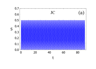
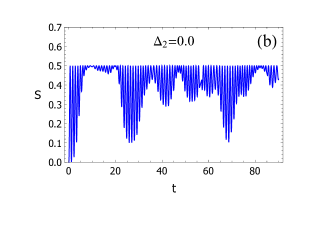
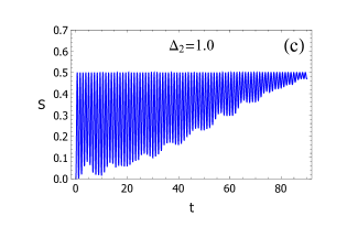
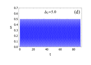
Figure 1: Linear entropy of atom 1 as a function of time. In (a) the field is not coupled to the environment, i.e., $\lambda_{2}=0.0$ (Jaynes Cummings model). For the field coupled to the environment, with $\lambda_{2}=0.1$ and (b) $\Delta_{2}=0.0$; (c) $\Delta_{2}=1.0$, and (d) $\Delta_{2}=5.0$. In all cases $\lambda_{1}=1.0$, and the initial state of the system is a tripartite product state with $\left|\psi_{a1}\right\rangle=\left|e_{1}\right\rangle$, $\rho_{a2}=\frac{1}{2}\left(\left|g_{2}\right\rangle\left\langle g_{2}\right|+\left|e_{2}\right\rangle\left\langle e_{2}\right|\right)$ and $\left|\psi_{f}\right\rangle=\left|1\right\rangle$.

We would like now to analyze the effect of $\Delta_{2}$ (atom 2-field detuning) on the time evolution of the linear entropy of atom 1. In figure (1) we have plots of the linear entropy of atom 1 as a function of time considering different values of $\Delta_{2}$. The field is initially prepared in the one photon Fock state $\left|1\right\rangle$, atom 1 in its excited state $|e_{1}\rangle$, and atom 2 in a maximally mixed state, $\rho_{a2}(0)=\frac{1}{2}\left(\left|g_{2}\right\rangle\left\langle g_{2}\right|+\left|e_{2}\right\rangle\left\langle e_{2}\right|\right)$.

As seen in figure (1a), the linear entropy is a periodic function of time (Rabi oscillations) if atom 2 is decoupled from the field, i.e., for $\lambda_{2}=0.0$. If the interaction between atom 2 and the field is turned on ($\lambda_{2}=0.1$), the evolution of the linear entropy becomes very irregular, as shown in figure (1b), which characterizes a destructive effect due to an unwanted coupling to a noisy sub-system. Nevertheless, it is possible to restore periodicity by controlling the atom 2-field frequency detuning. If $\Delta_{2}$ is increased, we expect less influence of atom 2 over the dynamics of the system of interest. In fact, as shown in figure (1c) and figure (1d), periodicity may be re-established for a sufficiently large $\Delta_{2}$. We remark that atom 1 is kept on resonance with the field ($\Delta_{1}=0.0$) as well as strongly coupled to it ($\lambda_{1}=1.0$).

3.2 Reduced dynamics of atom 1: atomic dipole squeezing

Atomic dipole squeezing is a non-classical effect that may arise in the Jaynes-Cummings model [16]. An atom is said to be dipole squeezed if the quantum fluctuations of the atomic dipole are below the fundamental limit imposed by the Heisenberg inequalities. The components of the (slowly varying) atomic dipole operator (for atom 1) may be written as [16]

$$\sigma_{x} = \sigma_{1}^{+}e^{i\omega_{1}t}+\sigma_{1}^{-}e^{-i\omega_{1}t}\,,$$

$$\sigma_{y} = \frac{1}{i}\left(\sigma_{1}^{+}e^{i\omega_{1}t}-\sigma_{1}^{-}e^{-i\omega_{1}t}\right)\,.$$ (14)

The operators above do not commute ($\left[\sigma_{x},\sigma_{y}\right]=2i\,\sigma_{z}$), and thus they should obey the Heisenberg inequality $\left(\Delta\sigma_{x}\right)\left(\Delta\sigma_{y}\right)\geq\left|\left\langle\sigma_{z}\right\rangle\right|$. Atomic dipole squeezing is verified if

$$\left(\Delta\sigma_{x,\,y}\right)^{2}<\left|\left\langle\sigma_{z}\right\rangle\right|\,,$$ (15)

where $\left(\Delta\sigma_{x}\right)^{2}=1-4\left(Re\left\langle\sigma_{1}^{-}\right\rangle e^{-i\,\omega_{1}t}\right)^{2}$ and $\left(\Delta\sigma_{y}\right)^{2}=1-4\left(Im\left\langle\sigma_{1}^{-}\right\rangle e^{-i\,\omega_{1}t}\right)^{2}$. The conditions for squeezing may be written in terms of the functions $s_{1}$ e $s_{2}$ (indexes of squeezing) as

$$s_{1}=\frac{1-4\left(Re\left\langle\sigma_{1}^{-}\right\rangle e^{-i\,\omega_{1}t}\right)^{2}}{\left|\left\langle\sigma_{z}\right\rangle\right|}<1\quad\mbox{or}\quad s_{2}=\frac{1-4\left(Im\left\langle\sigma_{1}^{-}\right\rangle e^{-i\,\omega_{1}t}\right)^{2}}{\left|\left\langle\sigma_{z}\right\rangle\right|}<1\;,$$ (16)

where $\omega_{1}$ is the frequency of atom 1, and $\left\langle\sigma_{z}\right\rangle$ is its corresponding atomic inversion. Here $\left\langle\sigma_{\alpha}\right\rangle=Tr_{1}\left(\sigma_{\alpha}\rho_{a1}\right)$.

We may rewrite the indexes of squeezing, $s_{1}$ and $s_{2}$, in terms of the functions $\alpha(t)$ and $\gamma(t)$ above, or

$$s_{1} = \frac{1-4\left(Re[\gamma]\cos\left(\omega_{1}t\right)-Im[\gamma]\sin\left(\omega_{1}t\right)\right)^{2}}{\left|1-2\alpha\left(t\right)\right|}<1\quad,$$

$$s_{2} = \frac{1-4\left(Re[\gamma]\sin\left(\omega_{1}t\right)+Im[\gamma]\cos\left(\omega_{1}t\right)\right)^{2}}{\left|1-2\alpha\left(t\right)\right|}<1\;.$$ (17)

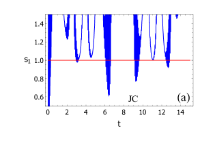
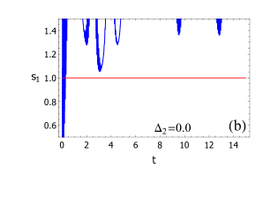
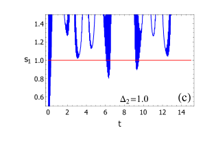
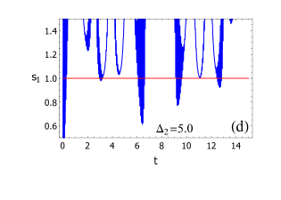
Figure 2: Squeezing index $s_{1}$ as a function of time. In (a) the field is not coupled to the environment, i.e., $\lambda_{2}=0.0$ (Jaynes Cummings model). For the field coupled to the environment, with $\lambda_{2}=0.1$ and (b) $\Delta_{2}=0.0$; (c) $\Delta_{2}=1.0$, and (d) $\Delta_{2}=5.0$. In all cases $\lambda_{1}=1.0$, and the initial state of the system is a tripartite product state with$\left|\psi_{a1}\right\rangle=\cos\left(0.6\right)\left|g_{1}\right\rangle+\sin\left(0.6\right)\left|e_{1}\right\rangle$, $\rho_{a2}=\frac{1}{2}\left(\left|g_{2}\right\rangle\left\langle g_{2}\right|+\left|e_{2}\right\rangle\left\langle e_{2}\right|\right)$ and $\left|\psi_{f}\right\rangle=\left|1\right\rangle$.

Now we choose specific initial conditions which allow dipole squeezing in the case of having atom 2 completely decoupled from the field ($\lambda_{2}=0.0$), which corresponds to the Jaynes-Cummings model. Atom 1 is assumed to be prepared in the superposition state $\left|\phi_{1}(0)\right\rangle=\cos\left(0.6\right)\left|g_{1}\right\rangle+\sin\left(0.6\right)\left|e_{1}\right\rangle$; atom 2 in the maximally mixed state, and the field in the one photon Fock state, $\left|1\right\rangle$. In figure (2) we have plotted the dipole squeezing index $s_{1}$ relative to atom 1 as a function of time. We note that in the absence of the “environment” (atom 2), dipole squeezing occurs for a few narrow intervals of time [figure (2a)]. If atom 2 is weakly coupled to the field, e.g., $\lambda_{2}=0.1$, the dipole squeezing is inhibited due to the action of the environment [see figure (2b)]. Yet, similarly to what we have seen in the previous subsection, dipole squeezing may be restored for a large enough detuning between atom 2 and the field, as shown in figures (2c) and (2d).

3.3 Atom 1-field entanglement

We may quantify the entanglement between atom 1 and the field by evaluating the negativity [21], an entanglement measure convenient in this case. Now we assume the following initial conditions: the field initially prepared in the vacuum state $\left|0\right\rangle$, atom 1 in its excited state $|e_{1}\rangle$, and atom 2 in a maximally mixed state. The negativity may be calculated from the time-dependent atom 1-field reduced density operator

$$\rho_{a1-f}\left(t\right) = \rho_{11}\left|g_{1},0\right\rangle\left\langle g_{1},0\right|+\rho_{22}\left|g_{1},1\right\rangle\left\langle g_{1},1\right|+\rho_{33}\left|g_{1},2\right\rangle\left\langle g_{1},2\right|+$$

$$+\rho_{44}\left|e_{1},0\right\rangle\left\langle e_{1},0\right|+\rho_{55}\left|e_{1},1\right\rangle\left\langle e_{1},1\right|+\rho_{24}\left|g_{1},1\right\rangle\left\langle e_{1},0\right|+$$

$$+\rho_{24}^{*}\left|e_{1},0\right\rangle\left\langle g_{1},1\right|+\rho_{35}\left|g_{1},2\right\rangle\left\langle e_{1},1\right|+\rho_{35}^{*}\left|e_{1},1\right\rangle\left\langle g_{1},2\right|.$$

The relevant matrix elements are

$$\rho_{11}=\frac{1}{2}\left|C_{3,-1}^{\left(II\right)}\right|^{2}\,,\quad\quad\rho_{22}=\frac{1}{2}\left(\left|C_{3,0}^{\left(I\right)}\right|^{2}+\left|C_{4,-1}^{\left(II\right)}\right|^{2}\right)\,,$$

$$\rho_{33}=\frac{1}{2}\left|C_{4,0}^{\left(I\right)}\right|^{2}\,,\qquad\rho_{44}=\frac{1}{2}\left(\left|C_{1,0}^{\left(I\right)}\right|^{2}+\left|C_{2,-1}^{\left(II\right)}\right|^{2}\right)\,,$$

$$\rho_{55}=\frac{1}{2}\left|C_{2,0}^{\left(I\right)}\right|^{2}\,,\qquad\rho_{35}=\frac{1}{2}\left(C_{2,0}^{\left(I\right)}\right)^{*}C_{4,0}^{\left(I\right)}\,,$$

$$\rho_{24}=\frac{1}{2}\left[\left(C_{1,0}^{\left(I\right)}\right)^{*}C_{3,0}^{\left(I\right)}+\left(C_{2,-1}^{\left(II\right)}\right)^{*}C_{4,-1}^{\left(II\right)}\right]\,.$$

Thus the negativity $\mathcal{N}$ may be expressed as

$$\mathcal{N}=2\sum_{i=1}^{2}\left|a_{i}\right|$$

$$a_{1}=\frac{1}{2}\left(\rho_{22}-\sqrt{\rho_{22}^{2}+4\left|\rho_{35}\right|^{2}}\right)\,,\qquad a_{2}=\frac{1}{2}\left(\rho_{11}+\rho_{55}-\sqrt{(\rho_{11}-\rho_{55})^{2}+4\left|\rho_{24}\right|^{2}}\right)\,.$$

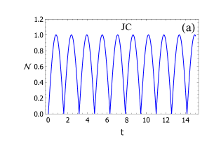
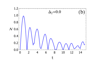
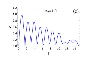
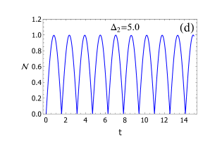
Figure 3: Negativity $\cal{N}$ used to quantify the entanglement between atom 1 and the field as a function of time. In (a) the field is not coupled to the environment, i.e., $\lambda_{2}=0.0$ (Jaynes Cummings model). For the field coupled to the environment, with $\lambda_{2}=0.2$ and (b) $\Delta_{2}=0.0$; (c) $\Delta_{2}=1.0$, and (d) $\Delta_{2}=5.0$. In all cases $\lambda_{1}=1.0$, and the initial state of the system is a tripartite product state with $\left|\psi_{a1}\right\rangle=\left|e_{1}\right\rangle$, $\rho_{a2}=\frac{1}{2}\left(\left|g_{2}\right\rangle\left\langle g_{2}\right|+\left|e_{2}\right\rangle\left\langle e_{2}\right|\right)$ and $\left|\psi_{f}\right\rangle=\left|0\right\rangle$.

We have inserted a factor of $2$ so that the maximum entanglement corresponds to $\mathcal{N}=1$. We note that although the negativity is somehow related to the linear entropy, they may not have the same behaviour, given that in this case the reduced atom 1-field density operator is obtained from a mixed state. In figure (3) we have plotted the negativity $\cal{N}$ as a function of time. For the initial conditions chosen here, the system has a simple evolution, i.e., a oscillatory behaviour as shown in figure (3a), provided the system is isolated (decoupled environment). However, if atom 2 (environment) is resonantly coupled to the field, the entanglement is severely damped [see figure (3b)], similarly to what happens to the linear entropy and atomic dipole squeezing. Again, entanglement may be restored if $\Delta_{2}$ is increased, as shown in figures (3c) and (3d).

4 Time-averaged evolution of the linear entropy

Now we would like to estimate the influence of the degree of mixedness of the small environment in the decoherence process. A simple way of doing that is for instance by calculating the time average of the linear entropy, here denoted as $S_{T}$ and defined as

$$S_{T}\left(T\right)=\frac{1}{T}\int_{0}^{T}S\left(t\right)dt,$$ (18)

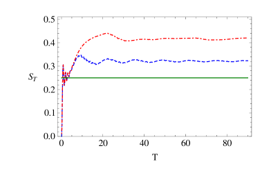
Figure 4: Time-averaged linear entropy ($S_{T}$) of atom 1, as a function of time for a) $p=0.0$ dashed (blue) curve, and b) $p=0.5$ dot-dashed (red) curve. In both cases $\lambda_{1}=1.0$, $\lambda_{2}=0.1$ and $\Delta_{1}=\Delta_{2}=0.0$. We also have $\left|\psi_{a1}\right\rangle=\left|e_{1}\right\rangle$, $\rho_{a2}=p\left|e_{2}\right\rangle\left\langle e_{2}\right|+(1-p)\left|g_{2}\right\rangle\left\langle g_{2}\right|$ and $\left|\psi_{f}\right\rangle=\left|1\right\rangle$. The continuous green line is drawn for $S_{T}=0.25$, corresponding to the uncoupled case, or $\lambda_{2}=0.0$

where $S(t)$ the linear entropy in equation (10). We are not including the resulting expression for $S_{T}$ because it is a rather large one. We calculated the time average of the linear entropy of atom 1 in two distinct situations; for atom 2 initially i) in a pure state ($p=0.0$) and ii) in a maximally mixed state ($p=0.5$). Naturally, larger values of $S_{T}$ (steady state) are an indication of larger degradation of quantum coherence. In figure 4 we have plotted $S_{T}$ (defined above) as a function of time ($T$). The dashed (blue) curve is for $p=0.0$ and the dot-dashed (red) curve for $p=0.5$. The influence of the degree of mixedness of the small environment on the state purity of atom 1 is clear, as we note that there is a significant increase ($\sim 30\%$) in its linear entropy (for long times), if the small environment is initially in a maximally mixed state ($p=0.5$) rather than in a pure state ($p=0.0$). Note that the average value of the linear entropy in the absence of an environment ($\lambda_{2}=0.0$) is $S_{0}=0.25$ (continuous green line in the plot). We would like to remark that a time averaging procedure may also be useful to discuss the effects of additional external fluctuations. Interestingly, solely by performing some kind of time-averaging it is possible to build a model for non-dissipative decoherence, as described in reference [22]. Also, a long-time average of the density operator allows the investigation of the thermalization properties of systems having a small number of degrees of freedom, as shown in [23].

5 Conclusions

We have presented a study of the dynamics of a bipartite quantum system (atom 1$+$field) in which the field is weakly coupled ($\lambda_{2}\approx\lambda_{1}/10$) to a small environment (atom 2). A single atom corresponds to the smallest possible environment considering the atomic beam model for a reservoir [5]. Of course there is no relaxation in this simple model, contrarily to what happens in the case of a “many atoms reservoir”. Instead, due to the incommensurate frequencies characteristic of the model, we expect quasi-recurrences of the considered physical quantities at longer time-scales. For instance, as we have seen, the linear entropy of atom 1 undergoes an irreversible-like evolution. We have also investigated the evolution of quantities related to non-classical behaviour, such as the dipole squeezing of atom 1 and the negativity, which quantifies the atom 1-field quantum entanglement. We have found that both the atomic dipole squeezing and the atom 1-field entanglement are considerably degraded at shorter time scales (especially in the resonant case, $\Delta_{2}=0.0$). In particular, we have verified that dipole squeezing, which occurs at relatively narrow time intervals, is completely suppressed. Of course due to the nature of the toy model here studied, there might occur quasi-revivals at longer times. However, even if a small amount of noise is added to the system, the joint action of the minimal environment and the extra noise could completely destroy the above mentioned quantum properties, as discussed in [10].

Here we have studied a general case, by analytically solving the two-atom TCM for non-identical atoms, with different coupling constants, ($\lambda_{1}\neq\lambda_{2}$) and different detunings ($\Delta_{1}\neq\Delta_{2}$). The solution of the two-atom TCM for non-identical atoms allowed us to assess the effect of the atom 2-field detuning on the dynamics of the system. Indeed there is a competition between the field-environment coupling and the field-environment detuning, but although we were able to determine explicitly the dependence of the quantum state of the system on the parameters ($\lambda_{1},\lambda_{2},\Delta_{1},\Delta_{2}$), the lengthy expressions hindered a more detailed analysis. We have shown that it is possible to have some degree of control over the dynamics of the system and circumvent the destructive effect of the environment. By increasing the atom 2-field detuning $\Delta_{2}$, there will be an effective decoupling of the small environment, and we expect a restoration of the non-classical properties such as squeezing and entanglement. For instance, if $\Delta_{2}=1.0$ it is possible to recover the atomic dipole squeezing property of atom 1. Yet, larger values of detuning would be required to restore the atom-field entanglement, as it is clearly seen in figure (3).

We have also made an estimate of the influence of the degree of mixedness of the small environment on the evolution of the main system by calculating the time-average of the linear entropy for different effective temperatures of the environment.

Appendix. Solution of the two-atom Tavis-Cummings model

Here we present the full analytical solution of the two-atom Tavis-Cummings model (coefficients $A_{kl}$). The diagonal terms are

$$A_{11}=\frac{1}{54}\left\{\frac{e^{-\frac{1}{2}t\left(\sqrt{X}-\sqrt{Y_{1}}\right)}\left(18\left(\sqrt{3}+i\right)D_{1}J_{1}\left(-2ik_{1}+3\sqrt{X}-3\sqrt{Y_{1}}\right)-432D_{1}^{3}-4iJ_{1}^{3}+\left(2ik_{1}-3\sqrt{X}+3\sqrt{Y_{1}}\right){}^{3}\right)}{\sqrt{Y_{1}}\left(-4\sqrt{X}\sqrt{Y_{1}}+4X+Y_{1}-Y_{2}\right)}\right.$$

$$+\frac{e^{-\frac{1}{2}t\left(\sqrt{X}+\sqrt{Y_{1}}\right)}\left(18\left(\sqrt{3}+i\right)iD_{1}J_{1}\left(2k_{1}+3i\left(\sqrt{X}+\sqrt{Y_{1}}\right)\right)+432D_{1}^{3}+i\left(4J_{1}^{3}+\left(2k_{1}+3i\left(\sqrt{X}+\sqrt{Y_{1}}\right)\right){}^{3}\right)\right)}{\sqrt{Y_{1}}\left(4\sqrt{X}\sqrt{Y_{1}}+4X+Y_{1}-Y_{2}\right)}$$

$$+\frac{e^{\frac{1}{2}t\left(\sqrt{X}-\sqrt{Y_{2}}\right)}\left(18\left(\sqrt{3}+i\right)D_{1}J_{1}\left(2ik_{1}+3\sqrt{X}-3\sqrt{Y_{2}}\right)+432D_{1}^{3}+4iJ_{1}^{3}+\left(-2ik_{1}-3\sqrt{X}+3\sqrt{Y_{2}}\right){}^{3}\right)}{\sqrt{Y_{2}}\left(-4\sqrt{X}\sqrt{Y_{2}}+4X-Y_{1}+Y_{2}\right)}$$

$$\left.+\frac{e^{\frac{1}{2}t\left(\sqrt{X}+\sqrt{Y_{2}}\right)}\left(18\left(1-i\sqrt{3}\right)D_{1}J_{1}\left(2k_{1}-3i\left(\sqrt{X}+\sqrt{Y_{2}}\right)\right)-432D_{1}^{3}-i\left(4J_{1}^{3}+\left(2k_{1}-3i\left(\sqrt{X}+\sqrt{Y_{2}}\right)\right){}^{3}\right)\right)}{\sqrt{Y_{2}}\left(4\sqrt{X}\sqrt{Y_{2}}+4X-Y_{1}+Y_{2}\right)}\right\},$$

$$A_{22}=\frac{1}{54}\left\{\frac{e^{-\frac{1}{2}t\left(\sqrt{X}-\sqrt{Y_{1}}\right)}\left(18\left(\sqrt{3}+i\right)D_{2}J_{2}\left(-2ik_{2}+3\sqrt{X}-3\sqrt{Y_{1}}\right)-432D_{2}^{3}-4iJ_{2}^{3}+\left(2ik_{2}-3\sqrt{X}+3\sqrt{Y_{1}}\right){}^{3}\right)}{\sqrt{Y_{1}}\left(-4\sqrt{X}\sqrt{Y_{1}}+4X+Y_{1}-Y_{2}\right)}\right.$$

$$+\frac{e^{-\frac{1}{2}t\left(\sqrt{X}+\sqrt{Y_{1}}\right)}\left(18\left(\sqrt{3}+i\right)iD_{2}J_{2}\left(2k_{2}+3i\left(\sqrt{X}+\sqrt{Y_{1}}\right)\right)+432D_{2}^{3}+i\left(4J_{2}^{3}+\left(2k_{2}+3i\left(\sqrt{X}+\sqrt{Y_{1}}\right)\right){}^{3}\right)\right)}{\sqrt{Y_{1}}\left(4\sqrt{X}\sqrt{Y_{1}}+4X+Y_{1}-Y_{2}\right)}$$

$$+\frac{e^{\frac{1}{2}t\left(\sqrt{X}-\sqrt{Y_{2}}\right)}\left(18\left(\sqrt{3}+i\right)D_{2}J_{2}\left(2ik_{2}+3\sqrt{X}-3\sqrt{Y_{2}}\right)+432D_{2}^{3}+4iJ_{2}^{3}+\left(-2ik_{2}-3\sqrt{X}+3\sqrt{Y_{2}}\right){}^{3}\right)}{\sqrt{Y_{2}}\left(-4\sqrt{X}\sqrt{Y_{2}}+4X-Y_{1}+Y_{2}\right)}$$

$$\left.+\frac{e^{\frac{1}{2}t\left(\sqrt{X}+\sqrt{Y_{2}}\right)}\left(18\left(1-i\sqrt{3}\right)D_{2}J_{2}\left(2k_{2}-3i\left(\sqrt{X}+\sqrt{Y_{2}}\right)\right)-432D_{2}^{3}-i\left(4J_{2}^{3}+\left(2k_{2}-3i\left(\sqrt{X}+\sqrt{Y_{2}}\right)\right){}^{3}\right)\right)}{\sqrt{Y_{2}}\left(4\sqrt{X}\sqrt{Y_{2}}+4X-Y_{1}+Y_{2}\right)}\right\},$$

$$A_{33}=\frac{1}{54}\left\{\frac{e^{-\frac{1}{2}t\left(\sqrt{X}-\sqrt{Y_{1}}\right)}\left(18\left(\sqrt{3}+i\right)D_{3}J_{3}\left(-2ik_{3}+3\sqrt{X}-3\sqrt{Y_{1}}\right)-432D_{3}^{3}-4iJ_{3}^{3}+\left(2ik_{3}-3\sqrt{X}+3\sqrt{Y_{1}}\right){}^{3}\right)}{\sqrt{Y_{1}}\left(-4\sqrt{X}\sqrt{Y_{1}}+4X+Y_{1}-Y_{2}\right)}\right.$$

$$+\frac{e^{-\frac{1}{2}t\left(\sqrt{X}+\sqrt{Y_{1}}\right)}\left(18\left(\sqrt{3}+i\right)iD_{3}J_{3}\left(2k_{3}+3i\left(\sqrt{X}+\sqrt{Y_{1}}\right)\right)+432D_{3}^{3}+i\left(4J_{3}^{3}+\left(2k_{3}+3i\left(\sqrt{X}+\sqrt{Y_{1}}\right)\right){}^{3}\right)\right)}{\sqrt{Y_{1}}\left(4\sqrt{X}\sqrt{Y_{1}}+4X+Y_{1}-Y_{2}\right)}$$

$$+\frac{e^{\frac{1}{2}t\left(\sqrt{X}-\sqrt{Y_{2}}\right)}\left(18\left(\sqrt{3}+i\right)D_{3}J_{3}\left(2ik_{3}+3\sqrt{X}-3\sqrt{Y_{2}}\right)+432D_{3}^{3}+4iJ_{3}^{3}+\left(-2ik_{3}-3\sqrt{X}+3\sqrt{Y_{2}}\right){}^{3}\right)}{\sqrt{Y_{2}}\left(-4\sqrt{X}\sqrt{Y_{2}}+4X-Y_{1}+Y_{2}\right)}$$

$$\left.+\frac{e^{\frac{1}{2}t\left(\sqrt{X}+\sqrt{Y_{2}}\right)}\left(18\left(1-i\sqrt{3}\right)D_{3}J_{3}\left(2k_{3}-3i\left(\sqrt{X}+\sqrt{Y_{2}}\right)\right)-432D_{3}^{3}-i\left(4J_{3}^{3}+\left(2k_{3}-3i\left(\sqrt{X}+\sqrt{Y_{2}}\right)\right){}^{3}\right)\right)}{\sqrt{Y_{2}}\left(4\sqrt{X}\sqrt{Y_{2}}+4X-Y_{1}+Y_{2}\right)}\right\},$$

$$A_{44}=\frac{1}{54}\left\{\frac{e^{-\frac{1}{2}t\left(\sqrt{X}-\sqrt{Y_{1}}\right)}\left(18\left(\sqrt{3}+i\right)D_{4}J_{4}\left(-2ik_{4}+3\sqrt{X}-3\sqrt{Y_{1}}\right)-432D_{4}^{3}-4iJ_{4}^{3}+\left(2ik_{4}-3\sqrt{X}+3\sqrt{Y_{1}}\right){}^{3}\right)}{\sqrt{Y_{1}}\left(-4\sqrt{X}\sqrt{Y_{1}}+4X+Y_{1}-Y_{2}\right)}\right.$$

$$+\frac{e^{-\frac{1}{2}t\left(\sqrt{X}+\sqrt{Y_{1}}\right)}\left(18\left(\sqrt{3}+i\right)iD_{4}J_{4}\left(2k_{4}+3i\left(\sqrt{X}+\sqrt{Y_{1}}\right)\right)+432D_{4}^{3}+i\left(4J_{4}^{3}+\left(2k_{4}+3i\left(\sqrt{X}+\sqrt{Y_{1}}\right)\right){}^{3}\right)\right)}{\sqrt{Y_{1}}\left(4\sqrt{X}\sqrt{Y_{1}}+4X+Y_{1}-Y_{2}\right)}$$

$$+\frac{e^{\frac{1}{2}t\left(\sqrt{X}-\sqrt{Y_{2}}\right)}\left(18\left(\sqrt{3}+i\right)D_{4}J_{4}\left(2ik_{4}+3\sqrt{X}-3\sqrt{Y_{2}}\right)+432D_{4}^{3}+4iJ_{4}^{3}+\left(-2ik_{4}-3\sqrt{X}+3\sqrt{Y_{2}}\right){}^{3}\right)}{\sqrt{Y_{2}}\left(-4\sqrt{X}\sqrt{Y_{2}}+4X-Y_{1}+Y_{2}\right)}$$

$$\left.+\frac{e^{\frac{1}{2}t\left(\sqrt{X}+\sqrt{Y_{2}}\right)}\left(18\left(1-i\sqrt{3}\right)D_{4}J_{4}\left(2k_{4}-3i\left(\sqrt{X}+\sqrt{Y_{2}}\right)\right)-432D_{4}^{3}-i\left(4J_{4}^{3}+\left(2k_{4}-3i\left(\sqrt{X}+\sqrt{Y_{2}}\right)\right){}^{3}\right)\right)}{\sqrt{Y_{2}}\left(4\sqrt{X}\sqrt{Y_{2}}+4X-Y_{1}+Y_{2}\right)}\right\},$$

and the non-diagonal terms read

$$A_{14}=-4\lambda_{1}\lambda_{2}\sqrt{(n+1)(n+2)}\left\{\frac{\left(\sqrt{Y_{1}}-\sqrt{X}\right)e^{-\frac{1}{2}t\left(\sqrt{X}-\sqrt{Y_{1}}\right)}}{\sqrt{Y_{1}}\left(-4\sqrt{X}\sqrt{Y_{1}}+4X+Y_{1}-Y_{2}\right)}+\frac{\left(\sqrt{X}+\sqrt{Y_{1}}\right)e^{-\frac{1}{2}t\left(\sqrt{X}+\sqrt{Y_{1}}\right)}}{\sqrt{Y_{1}}\left(4\sqrt{X}\sqrt{Y_{1}}+4X+Y_{1}-Y_{2}\right)}\right.$$

$$\left.+\frac{\left(\sqrt{X}+\sqrt{Y_{2}}\right)e^{\frac{1}{2}t\left(\sqrt{X}+\sqrt{Y_{2}}\right)}}{\sqrt{Y_{2}}\left(4\sqrt{X}\sqrt{Y_{2}}+4X-Y_{1}+Y_{2}\right)}+\frac{\left(\sqrt{Y_{2}}-\sqrt{X}\right)e^{\frac{1}{2}t\left(\sqrt{X}-\sqrt{Y_{2}}\right)}}{\sqrt{Y_{2}}\left(-4\sqrt{X}\sqrt{Y_{2}}+4X-Y_{1}+Y_{2}\right)}\right\},$$

$$A_{23}=-\frac{2e^{\frac{1}{2}t\left(\sqrt{X}+\sqrt{Y_{2}}\right)}\left(i\left(\Delta_{1}+\Delta_{2}\right)\lambda_{1}\lambda_{2}+(2n+3)\sqrt{X}+(2n+3)\sqrt{Y_{2}}\right)}{\sqrt{Y_{2}}\left(4\sqrt{X}\sqrt{Y_{2}}+4X-Y_{1}+Y_{2}\right)}$$

$$+\frac{e^{-\frac{1}{2}t\left(\sqrt{X}+\sqrt{Y_{1}}\right)}\left(2i\left(\Delta_{1}+\Delta_{2}\right)\lambda_{1}\lambda_{2}-2(2n+3)\sqrt{X}-2(2n+3)\sqrt{Y_{1}}\right)}{\sqrt{Y_{1}}\left(4\sqrt{X}\sqrt{Y_{1}}+4X+Y_{1}-Y_{2}\right)}$$

$$+\frac{e^{\frac{1}{2}t\left(\sqrt{X}-\sqrt{Y_{2}}\right)}\left(2i\left(\Delta_{1}+\Delta_{2}\right)\lambda_{1}\lambda_{2}+(4n+6)\sqrt{X}-2(2n+3)\sqrt{Y_{2}}\right)}{\sqrt{Y_{2}}\left(-4\sqrt{X}\sqrt{Y_{2}}+4X-Y_{1}+Y_{2}\right)}$$

$$+\frac{e^{-\frac{1}{2}t\left(\sqrt{X}-\sqrt{Y_{1}}\right)}\left((4n+6)\sqrt{X}-2\left((2n+3)\sqrt{Y_{1}}+i\left(\Delta_{1}+\Delta_{2}\right)\lambda_{1}\lambda_{2}\right)\right)}{\sqrt{Y_{1}}\left(-4\sqrt{X}\sqrt{Y_{1}}+4X+Y_{1}-Y_{2}\right)},$$

$$A_{13}=-i\lambda_{1}\sqrt{n+1}\left\{-\frac{e^{\frac{1}{2}t\left(\sqrt{X}-\sqrt{Y_{2}}\right)}\left(G+\left(\sqrt{X}-\sqrt{Y_{2}}\right)\left(-2i\Delta_{2}+\sqrt{X}-\sqrt{Y_{2}}\right)\right)}{\sqrt{Y_{2}}\left(-4\sqrt{X}\sqrt{Y_{2}}+4X-Y_{1}+Y_{2}\right)}\right.$$

$$+\frac{e^{\frac{1}{2}t\left(\sqrt{X}+\sqrt{Y_{2}}\right)}\left(G+\left(\sqrt{X}+\sqrt{Y_{2}}\right)\left(-2i\Delta_{2}+\sqrt{X}+\sqrt{Y_{2}}\right)\right)}{\sqrt{Y_{2}}\left(4\sqrt{X}\sqrt{Y_{2}}+4X-Y_{1}+Y_{2}\right)}$$

$$+\frac{e^{-\frac{1}{2}t\left(\sqrt{X}-\sqrt{Y_{1}}\right)}\left(G+\left(\sqrt{X}-\sqrt{Y_{1}}\right)\left(2i\Delta_{2}+\sqrt{X}-\sqrt{Y_{1}}\right)\right)}{\sqrt{Y_{1}}\left(-4\sqrt{X}\sqrt{Y_{1}}+4X+Y_{1}-Y_{2}\right)}$$

$$\left.+\frac{e^{-\frac{1}{2}t\left(\sqrt{X}+\sqrt{Y_{1}}\right)}\left(-G-\left(\sqrt{X}+\sqrt{Y_{1}}\right)\left(2i\Delta_{2}+\sqrt{X}+\sqrt{Y_{1}}\right)\right)}{\sqrt{Y_{1}}\left(4\sqrt{X}\sqrt{Y_{1}}+4X+Y_{1}-Y_{2}\right)}\right\},$$

$$A_{12}=-i\sqrt{n+1}\lambda_{2}\left\{\frac{e^{\frac{1}{2}t\left(\sqrt{X}-\sqrt{Y_{2}}\right)}\left(G-\left(\sqrt{X}-\sqrt{Y_{2}}\right)\left(-2i\Delta_{1}+\sqrt{X}-\sqrt{Y_{2}}\right)\right)}{\sqrt{Y_{2}}\left(-4\sqrt{X}\sqrt{Y_{2}}+4X-Y_{1}+Y_{2}\right)}\right.$$

$$+\frac{e^{\frac{1}{2}t\left(\sqrt{X}+\sqrt{Y_{2}}\right)}\left(-G+\left(\sqrt{X}+\sqrt{Y_{2}}\right)\left(-2i\Delta_{1}+\sqrt{X}+\sqrt{Y_{2}}\right)\right)}{\sqrt{Y_{2}}\left(4\sqrt{X}\sqrt{Y_{2}}+4X-Y_{1}+Y_{2}\right)}$$

$$+\frac{e^{-\frac{1}{2}t\left(\sqrt{X}-\sqrt{Y_{1}}\right)}\left(-G+\left(\sqrt{X}-\sqrt{Y_{1}}\right)\left(2i\Delta_{1}+\sqrt{X}-\sqrt{Y_{1}}\right)\right)}{\sqrt{Y_{1}}\left(-4\sqrt{X}\sqrt{Y_{1}}+4X+Y_{1}-Y_{2}\right)}$$

$$\left.+\frac{e^{-\frac{1}{2}t\left(\sqrt{X}+\sqrt{Y_{1}}\right)}\left(G-\left(\sqrt{X}+\sqrt{Y_{1}}\right)\left(2i\Delta_{1}+\sqrt{X}+\sqrt{Y_{1}}\right)\right)}{\sqrt{Y_{1}}\left(4\sqrt{X}\sqrt{Y_{1}}+4X+Y_{1}-Y_{2}\right)}\right\},$$

$$A_{24}=-i\sqrt{n+2}\lambda_{1}\left\{\frac{e^{-\frac{1}{2}t\left(\sqrt{X}-\sqrt{Y_{1}}\right)}\left(H+\left(\sqrt{X}-\sqrt{Y_{1}}\right)\left(-2i\Delta_{2}+\sqrt{X}-\sqrt{Y_{1}}\right)\right)}{\sqrt{Y_{1}}\left(-4\sqrt{X}\sqrt{Y_{1}}+4X+Y_{1}-Y_{2}\right)}\right.$$

$$+\frac{e^{-\frac{1}{2}t\left(\sqrt{X}+\sqrt{Y_{1}}\right)}\left(-H-\left(\sqrt{X}+\sqrt{Y_{1}}\right)\left(-2i\Delta_{2}+\sqrt{X}+\sqrt{Y_{1}}\right)\right)}{\sqrt{Y_{1}}\left(4\sqrt{X}\sqrt{Y_{1}}+4X+Y_{1}-Y_{2}\right)}$$

$$+\frac{e^{\frac{1}{2}t\left(\sqrt{X}+\sqrt{Y_{2}}\right)}\left(H+\left(\sqrt{X}+\sqrt{Y_{2}}\right)\left(2i\Delta_{2}+\sqrt{X}+\sqrt{Y_{2}}\right)\right)}{\sqrt{Y_{2}}\left(4\sqrt{X}\sqrt{Y_{2}}+4X-Y_{1}+Y_{2}\right)}$$

$$\left.-\frac{e^{\frac{1}{2}t\left(\sqrt{X}-\sqrt{Y_{2}}\right)}\left(H+\left(\sqrt{X}-\sqrt{Y_{2}}\right)\left(2i\Delta_{2}+\sqrt{X}-\sqrt{Y_{2}}\right)\right)}{\sqrt{Y_{2}}\left(-4\sqrt{X}\sqrt{Y_{2}}+4X-Y_{1}+Y_{2}\right)}\right\},$$

$$A_{34}=-i\sqrt{n+2}\lambda_{2}\left\{\frac{e^{-\frac{1}{2}t\left(\sqrt{X}-\sqrt{Y_{1}}\right)}\left(-H+\left(\sqrt{X}-\sqrt{Y_{1}}\right)\left(-2i\Delta_{1}+\sqrt{X}-\sqrt{Y_{1}}\right)\right)}{\sqrt{Y_{1}}\left(-4\sqrt{X}\sqrt{Y_{1}}+4X+Y_{1}-Y_{2}\right)}\right.$$

$$+\frac{e^{-\frac{1}{2}t\left(\sqrt{X}+\sqrt{Y_{1}}\right)}\left(H-\left(\sqrt{X}+\sqrt{Y_{1}}\right)\left(-2i\Delta_{1}+\sqrt{X}+\sqrt{Y_{1}}\right)\right)}{\sqrt{Y_{1}}\left(4\sqrt{X}\sqrt{Y_{1}}+4X+Y_{1}-Y_{2}\right)}$$

$$+\frac{e^{\frac{1}{2}t\left(\sqrt{X}-\sqrt{Y_{2}}\right)}\left(H-\left(\sqrt{X}-\sqrt{Y_{2}}\right)\left(2i\Delta_{1}+\sqrt{X}-\sqrt{Y_{2}}\right)\right)}{\sqrt{Y_{2}}\left(-4\sqrt{X}\sqrt{Y_{2}}+4X-Y_{1}+Y_{2}\right)}$$

$$\left.+\frac{e^{\frac{1}{2}t\left(\sqrt{X}+\sqrt{Y_{2}}\right)}\left(-H+\left(\sqrt{X}+\sqrt{Y_{2}}\right)\left(2i\Delta_{1}+\sqrt{X}+\sqrt{Y_{2}}\right)\right)}{\sqrt{Y_{2}}\left(4\sqrt{X}\sqrt{Y_{2}}+4X-Y_{1}+Y_{2}\right)}\right\}.$$

In the expressions above, the coefficients $X$ and $Y_{1,\,2}$ are given by

$$X=-\frac{2A}{3}+\frac{2^{1/3}\left(A^{2}+12F\right)}{3\beta}+\frac{\Gamma}{3\times 2^{1/3}}$$

$$Y_{1,\,2}=-2A-X\pm\frac{2iB}{\sqrt{X}},$$

where

$$\Gamma=\left[2A^{3}-27B^{2}-72AF+\sqrt{-4\left(A^{2}+12F\right)^{3}+\left(2A^{3}-27B^{2}-72AF\right)^{2}}\right]^{1/3},$$

and

$$A=\frac{1}{2}\left(\Delta_{1}^{2}+\Delta_{2}^{2}+2(2n+3)\left(\lambda_{1}^{2}+\lambda_{2}^{2}\right)\right),$$

$$B=\left(\Delta_{1}\lambda_{2}^{2}+\Delta_{2}\lambda_{1}^{2}\right),$$

$$F = \frac{1}{16}\left\{\left(\Delta_{1}^{2}-\Delta_{2}^{2}\right)\left[\left(\Delta_{1}^{2}-\Delta_{2}^{2}\right)^{2}+4\left(3+2n\right)\left(\lambda_{1}^{2}-\lambda_{2}^{2}\right)\right]+16\left(n^{2}+3n+2\right)\left(\lambda_{1}^{2}-\lambda_{2}^{2}\right)^{2}\right\}.$$

We have also that

$$G=\Delta_{1}^{2}-\Delta_{2}^{2}+4\left(n+2\right)\left(\lambda_{1}^{2}-\lambda_{2}^{2}\right),$$

$$H=\Delta_{1}^{2}-\Delta_{2}^{2}+4\left(n+1\right)\left(\lambda_{1}^{2}-\lambda_{2}^{2}\right),$$

$$D_{i}=\frac{\left(-1\right)^{5/6}\left(3a_{i}+k_{i}^{2}\right)}{3J_{i}}\;,\quad i=1,\,2,\,3,\,4,$$

and

$$J_{i}=\left(-27b_{i}+9a_{i}k_{i}+2k_{i}^{3}-3i\sqrt{3}\sqrt{4a_{i}^{3}-27b_{i}^{2}+18a_{i}b_{i}k_{i}+a_{i}^{2}k_{i}^{2}+4b_{i}k_{i}^{3}}\right)^{1/3}\;,\quad i=1,\,2,\,3,\,4,$$

being

$$a_{1}=a_{4}=\frac{\left[\left(\Delta_{1}-\Delta_{2}\right)^{2}+4\left(n+2\right)\left(\lambda_{1}^{2}+\lambda_{2}^{2}\right)\right]}{4},$$

$$a_{2}=a_{3}=\frac{\left[\left(\Delta_{1}+\Delta_{2}\right)^{2}+4\left(\left(n+1\right)\lambda_{1}^{2}+\left(n+2\right)\lambda_{2}^{2}\right)\right]}{4},$$

$$b_{1}=-b_{4}=-\frac{\left(\Delta_{1}-\Delta_{2}\right)}{8}\left[\Delta_{1}^{2}-\Delta_{2}^{2}+4\left(n+2\right)\left(\lambda_{1}^{2}-\lambda_{2}^{2}\right)\right],$$

$$b_{2}=-b_{3}=-\frac{\left(\Delta_{1}+\Delta_{2}\right)}{8}\left[\Delta_{1}^{2}-\Delta_{2}^{2}+4\left(\left(n+1\right)\lambda_{1}^{2}-\left(n+2\right)\lambda_{2}^{2}\right)\right],$$

$$k_{1}=-k_{4}=-\frac{\left(\Delta_{1}+\Delta_{2}\right)}{2},$$

and

$$k_{2}=-k_{3}=-\frac{\left(\Delta_{1}-\Delta_{2}\right)}{2}.$$

References

- [1] Louisell, W.H. Quantum Statistical Properties of Radiation. John Wiley & Sons Inc, New York, 1973.
- [2] Caldeira A.O.; Leggett A.J. Influence of damping on quantum interference: An exactly soluble model. Phys. Rev. A 1985, 31, 1059.
- [3] Walls D.F.; Milburn G.J. Effect of dissipation on quantum coherence. Phys. Rev. A 1985, 31, 2403.
- [4] Joos E. et al., Decoherence and the Appearance of a Classical World in Quantum Theory, Springer-Verlag, Berlin, 1996.
- [5] Sargent M.; Scully M.O.; Lamb W.E. Laser Physics, Addison-Wesley, Reading (1974); Yamamoto Y.; İmamoğlu A. Mesoscopic Quantum Optics, John Wiley & Sons, Inc., New York, 1999.
- [6] Browne D.; Bose S.; Mintert F.; Kim M.S. From quantum optics to quantum technologies. Prog. Quantum Elec. 2017, 54, 2.
- [7] Barnett S. et al. Journeys from quantum optics to quantum technology. Prog. Quantum Elec. 2017, 54, 19.
- [8] Akoury D. et al., The Simplest Double Slit: Interference and Entanglement in Double Photoionization of . Science 2007, 318, 949.
- [9] Ingold G.-L.; Hänggi P.; Talkner P. Specific heat anomalies of open quantum systems. Phys. Rev. E 2009, 79, 061105.
- [10] Vidiella-Barranco A. Deviations from reversible dynamics in a qubit-oscillator system coupled to a very small environment. Physica A 2014, 402, 209.
- [11] Ashhab S. Landau-Zener transitions in a two-level system coupled to a finite-temperature harmonic oscillator. Phys. Rev. A 2014, 90, 062120.
- [12] Vidiella-Barranco A. Evolution of a quantum harmonic oscillator coupled to a minimal thermal environment. Physica A 2016, 459, 78.
- [13] Tavis M.; Cummings F.W. Exact Solution for an N-Molecule-Radiation-Field Hamiltonian. Phys. Rev. 1968, 170, 379.
- [14] Jaynes E.T.; Cummings F.W. Comparison of Quantum and Semiclassical Radiation Theories with Application to the Beam Maser. Proc. IEEE 1963, 51, 89.
- [15] Shore B.W.; Knight P.L. The Jaynes-Cummings model. J. Mod. Optics 1993, 40, 1195.
- [16] Walls D.F; Zoller P. Reduced Quantum Fluctuations in Resonance Fluorescence. Phys. Rev. Lett. 1981, 47, 709; Li X.S.; Lin D.L.; George T.F. Squeezing of atomic variables in the one-photon and two-photon Jaynes-Cummings model. Phys. Rev. A 1989, 40, 2504.
- [17] Maqbool T.; Razmi M.S.K.; Field and atomic dipole squeezing and emission spectra with two atoms in the cavity. J. Opt. Soc. Amer. B 1993, 10, 112.
- [18] Deng Z. Dynamics of two atoms in a quantized radiation field. Opt. Comm. 1985, 54, 222.
- [19] Mahmood S.; Zubairy M.S. Cooperative atomic interactions in a single-mode laser. Phys. Rev. A 1987, 35, 425.
- [20] Dung H.T; Huyen, N.D. Two Atom-single Mode Radiation Field Interaction. J. Mod. Optics 1994, 41, 453.
- [21] Życzkowski K.; Horodecki P.; Sanpera A.; Lewenstein M. Volume of the set of separable states. Phys. Rev. A 1998, 58, 883.
- [22] Bonifacio R.; Olivares S.; Tombesi P.; Vitali D. Model-independent approach to nondissipative decoherence. Phys. Rev. A 2000, 61, 053802.
- [23] Ikeda T.N.; Mori T.; Kaminishi E.; Ueda M. Entanglement prethermalization in an interaction quench between two harmonic oscillators. Phys. Rev. E 2017, 95, 022129.