Multi-dimensional Summation-By-Parts Operators:
General Theory and Application to Simplex Elements

Abstract

Summation-by-parts (SBP) finite-difference discretizations share many attractive properties with Galerkin finite-element methods (FEMs), including time stability and superconvergent functionals; however, unlike FEMs, SBP operators are not completely determined by a basis, so the potential exists to tailor SBP operators to meet different objectives. To date, application of high-order SBP discretizations to multiple dimensions has been limited to tensor product domains. This paper presents a definition for multi-dimensional SBP finite-difference operators that is a natural extension of one-dimensional SBP operators. Theoretical implications of the definition are investigated for the special case of a diagonal norm (mass) matrix. In particular, a diagonal-norm SBP operator exists on a given domain if and only if there is a cubature rule with positive weights on that domain and the polynomial-basis matrix has full rank when evaluated at the cubature nodes. Appropriate simultaneous-approximation terms are developed to impose boundary conditions weakly, and the resulting discretizations are shown to be time stable. Concrete examples of multi-dimensional SBP operators are constructed for the triangle and tetrahedron; similarities and differences with spectral-element and spectral-difference methods are discussed. An assembly process is described that builds diagonal-norm SBP operators on a global domain from element-level operators. Numerical results of linear advection on a doubly periodic domain demonstrate the accuracy and time stability of the simplex operators.

siscxxxxxxxx–x

1 Introduction

Summation-by-parts (SBP) operators are high-order finite-difference schemes that mimic the symmetry properties of the differential operators they approximate [19]. Respecting such symmetries has important implications; in particular, they enable SBP discretizations that are both time stable and high-order accurate [4, 34, 27], properties that are essential for robust, long-time simulations of turbulent flows [25, 35].

Most existing SBP operators are one-dimensional [30, 24, 31, 23] and are applied to multi-dimensional problems using a multi-block tensor-product formulation [32, 14, 29]. Like other tensor-product methods, the restriction to multi-block grids complicates mesh generation and adaptation, and it limits the geometric complexity that can be considered in practice.

The limitations of the tensor-product formulation motivate our interest in generalizing SBP operators to unstructured grids. There are two ways this generalization has been pursued in the literature: 1) construct global SBP operators on an arbitrary distribution of nodes, or; 2) construct SBP operators on reference elements and assemble a global discretization by coupling these smaller elements.

The first approach is appealing conceptually, and it is certainly viable for second-order accurate SBP schemes. For example, Nordström et al. [28] showed that the vertex-centered second-order-accurate finite-volume scheme has a multi-dimensional SBP property, even on unstructured grids; however, the first approach presents challenges when constructing high-order operators. Kitson et al. [17] showed that, for a given stencil width and design accuracy, there exist grids for which no stable, diagonal-norm SBP operator exists. Thus, building stable high-order SBP operators on arbitrary node distributions may require unacceptably large stencils. When SBP operators do exist for a given node distribution, they must be determined globally by solving a system of equations, in general. The global nature of these SBP operators is exemplified in the mesh-free framework of Chiu et al.[20, 5].

The second approach — constructing SBP operators on reference elements and using these to build the global discretization — is more common and presents fewer difficulties. The primary challenge here is to extend the one-dimensional SBP operators of Kreiss and Scherer [19] to a broader set of operators and domains. The existence of such operators, at least in the dense-norm case, was established by Carpenter and Gottlieb [2]. They proved that operators with the SBP property can be constructed from the Lagrangian interpolant on nearly arbitrary nodal distributions, which is practically feasible on reference elements with relatively few nodes. More recently, Gassner [10] showed that the discontinuous spectral-element method is equivalent to a diagonal-norm SBP discretization when the Legendre-Gauss-Lobatto nodes are used with a lumped mass matrix.

Of particular relevance to the present work is the extension of the SBP concept by Del Rey Fernandez et al.[7]. They introduced a generalized summation-by-parts (GSBP) definition for arbitrary node distributions on one-dimensional elements, and these ideas helped shape the definition of SBP operators presented herein.

Our first objective in the present work is to develop a suitable definition for multi-dimensional SBP operators on arbitrary grids and to characterize the resulting operators theoretically. We note that the discrete-derivative operator presented in [20] is a possible candidate for defining (diagonal-norm) multi-dimensional SBP operators; however, it lacks properties of conventional SBP operators that we would like to retain, such as the accuracy of the discrete divergence theorem [15].

Our second objective is to provide a concrete example of multi-dimensional diagonal-norm SBP operators on non-tensor-product domains. We focus on diagonal-norm operators, because they are better suited to discretizations that conserve non-quadratic invariants [17]; they are also more attractive than dense norms for explicit time-marching schemes. We construct diagonal-norm SBP operators for triangular and tetrahedral elements. The resulting operators are similar to those used in the nodal triangular-spectral-element method [6, 26, 11]. Unlike the spectral-element method based on cubature points, the SBP method is not completely specified by a polynomial basis; we use the resulting freedom to enforce the summation-by-parts property, which leads to provably time-stable schemes.

The remaining paper is structured as follows. Section 2 presents notation and the proposed definition for multi-dimensional SBP operators. We study the theoretical implications of the proposed definition in Section 3. We then describe, in Section 4, how to construct diagonal-norm SBP operators for the triangle and tetrahedron. Section 4 also establishes that SBP operators on subdomains can be assembled into SBP operators on the global domain. Results of applying the triangular SBP operators to the linear advection equation are presented in Section 5. Conclusions are given in Section 6.

2 Preliminaries

To make the presentation concise, we concentrate on multi-dimensional SBP operators in two dimensions; the extension to higher dimensions follows in a straightforward manner. Furthermore, we present definitions and theorems for operators in the $x$ coordinate direction only; the corresponding definitions and theorems for the $y$ coordinate direction follow directly from those in the $x$ direction.

2.1 Notation

We consider discretized derivative operators defined on a set of $n$ nodes, $S=\left\{(x_{i},y_{i})\right\}_{i=1}^{n}$. Capital letters with script type are used to denote continuous functions. For example, $\mathcal{U}(x)\in L^{2}(\Omega)$ denotes a square-integrable function on the domain $\Omega$. We use lower-case bold font to denote the restriction of functions to the nodes. Thus, the restriction of $\mathcal{U}$ to $S$ is given by

$$\bm{u}=\left[\mathcal{U}(x_{1},y_{1}),\dots,\mathcal{U}(x_{n},y_{n})\right]^{\mathrm{T}}.$$

Several theorems and proofs make use of the monomial basis. For two spatial variables, the size of the polynomial basis of total degree $p$ is

$$n^{*}_{p}\equiv\frac{(p+1)(p+2)}{2}.$$

More generally, $n^{*}_{p}=\binom{p+d}{d}$, where $d$ is the spatial dimension. We use the following single-subscript notation for monomial basis functions:

$$\mathcal{P}_{k}(x,y)\equiv x^{i}y^{j-i},\qquad k=j(j+1)/2+i+1,\quad\forall\;j\in\{0,1,\ldots,p\},\quad i\in\{0,1,\ldots,j\}.$$

We will frequently evaluate $\mathcal{P}_{k}$ and $\partial\mathcal{P}_{k}/\partial x$ at the nodes $S$, so we introduce the notation

$$\bm{p}_{k} \equiv\left[\mathcal{P}_{k}(x_{1},y_{1}),\dots,\mathcal{P}_{k}(x_{n},y_{n})\right]^{\mathrm{T}},$$

$$\text{and}\qquad\bm{p}_{k}^{\prime} \equiv\left[\frac{\partial\mathcal{P}_{k}}{\partial x}(x_{1},y_{1}),\dots,\frac{\partial\mathcal{P}_{k}}{\partial x}(x_{n},y_{n})\right]^{\mathrm{T}}.$$

Finally, matrices are represented using capital letters with sans-serif font; for example, the first-derivative operators with respect to $x$ and $y$ are represented by the matrices $\mathsf{D}_{x}$ and $\mathsf{D}_{y}$, respectively. Entries of a matrix are indicated with subscripts, and we follow Matlab^®-like notation when referencing submatrices. For example, $\mathsf{A}_{:,j}$ denotes the $j^{\text{th}}$ column of matrix $\mathsf{A}$, and $\mathsf{A}_{:,1:k}$ denotes its first $k$ columns.

2.2 Multi-dimensional SBP operator definition

We propose the following definition for $\mathsf{D}_{x}$, the SBP first-derivative operator with respect to $x$. An analogous definition holds for $\mathsf{D}_{y}$ and, in three-dimensions, $\mathsf{D}_{z}$. Definition 1 is a natural extension of the definition of GSBP operators proposed in [7], which itself extends the classical SBP operators introduced by Kreiss and Scherer [19].

Definition 1.

Two-dimensional summation-by-parts operator: Consider an open and bounded domain $\Omega\subset\mathbb{R}^{2}$ with a piecewise-smooth boundary $\Gamma$. The matrix $\mathsf{D}_{x}$ is a degree $p$ SBP approximation to the first derivative $\frac{\partial}{\partial x}$ on the nodes $S=\left\{(x_{i},y_{i})\right\}_{i=1}^{n}$ if

1. $\mathsf{D}_{x}\bm{p}_{k}=\bm{p}_{k}^{\prime},\qquad\forall\;k\in\{1,2,\ldots,n^{*}_{p}\}$;

2. $\mathsf{D}_{x}=\mathsf{H}^{-1}\mathsf{S}_{x}$, where $\mathsf{H}$ is symmetric positive-definite, and;

3. $\mathsf{S}_{x}=\mathsf{Q}_{x}+\frac{1}{2}\mathsf{E}_{x}$, where $\mathsf{Q}_{x}^{\mathrm{T}}=-\mathsf{Q}_{x}$, $\mathsf{E}_{x}^{\mathrm{T}}=\mathsf{E}_{x}$, and $\mathsf{E}_{x}$ satisfies

   $$\bm{p}_{k}^{\mathrm{T}}\mathsf{E}_{x}\bm{p}_{m}=\displaystyle\oint_{\Gamma}\mathcal{P}_{k}\mathcal{P}_{m}n_{x}\mathrm{d}\Gamma,\qquad\forall\;k,m\in\{1,2,\ldots,n^{*}_{\tau}\},$$

where $\tau\geq p$ and $n_{x}$ is the $x$ component of $\bm{n}=\left[n_{x},n_{y}\right]^{\mathrm{T}}$, the outward pointing unit normal on $\Gamma$.

Before studying the implications of Definition 1 in Section 3, it is worthwhile to motivate and elaborate on the three properties in the definition.

Property 1 ensures that $\mathsf{D}_{x}$ is an accurate approximation to the first partial derivative with respect to $x$. The operator must be exact for polynomials of total degree less than or equal to $p$, so at least $n^{*}_{p}$ nodes are necessary to satisfy property 1.

Remark 1.

We emphasize that a polynomial basis is not used to define the solution in SBP methods, in contrast with the piecewise polynomial expansions found in finite-element methods. We adopt the monomial basis only to define the accuracy conditions concisely and avoid cumbersome Taylor-series expansions.

The matrix $\mathsf{H}$ must be symmetric positive-definite to guarantee stability: without property 2, the discrete “energy”, $\bm{u}^{\mathrm{T}}\mathsf{H}\bm{u}$, could be negative when $\bm{u}^{\mathrm{T}}\bm{u}>0$, and vice versa. The so-called norm matrix $\mathsf{H}$ can be interpreted as a mass matrix, i.e.

$$\mathsf{H}_{i,j}=\int_{\Omega}\phi_{i}(x,y)\phi_{j}(x,y)\mathrm{d}\Omega,$$

but it is important to emphasize that SBP operators are finite-difference operators, and there is no (known) closed-form expression for an SBP nodal basis $\{\phi_{i}\}_{i=1}^{n}$, in general. In the diagonal norm case, we shall show that another interpretation of $\mathsf{H}$ is as a cubature rule.

Property 3 is needed to mimic integration by parts (IBP). Recall that the IBP formula for the $x$ derivative is

$$\int_{\Omega}\mathcal{V}\frac{\partial\mathcal{U}}{\partial x}\mathrm{d}\Omega+\int_{\Omega}\mathcal{U}\frac{\partial\mathcal{V}}{\partial x}\mathrm{d}\Omega=\oint_{\Gamma}\mathcal{V}\mathcal{U}n_{x}\mathrm{d}\Gamma.$$

The discrete version of the IBP formula, which follows from property 3, is

$$\bm{v}^{\mathrm{T}}\mathsf{H}\mathsf{D}_{x}\bm{u}+\bm{u}^{\mathrm{T}}\mathsf{H}\mathsf{D}_{x}\bm{v}=\bm{v}^{\mathrm{T}}\mathsf{E}_{x}\bm{u},\qquad\forall\;\bm{v},\bm{u}\in\mathbb{R}^{n}.$$

There is a one-to-one correspondence between each term in the IBP formula and its SBP proxy. For example, it is clear from property 3 that $\bm{v}^{\mathrm{T}}\mathsf{E}_{x}\bm{u}$ approximates the surface integral in IBP to order $\tau$. Moreover, in Section 3 we show that diagonal-norm SBP operators also approximate the left-hand side of IBP.

3 Analysis of diagonal-norm, multi-dimensional, summation-by-parts operators

In this section, we determine the implications of Definition 1 on the constituent matrices of a multi-dimensional SBP operator and whether or not such operators exist. We also investigate the time stability of discretizations based on multi-dimensional SBP operators. The focus is on diagonal-norm operators; however, the ideas presented here can be extended to dense-norm operators, i.e. where the matrix $\mathsf{H}$ is not diagonal.

The following lemma will prove useful in the sequel. It follows immediately from properties 1 and 3, so we state it without proof.

Lemma 2 (compatibility).

Let $\mathsf{D}_{x}=\mathsf{H}^{-1}(\mathsf{Q}_{x}+\frac{1}{2}\mathsf{E}_{x})$ be an SBP operator of degree $p$. Then we have the following set of relations:

$$\bm{p}_{m}^{\mathrm{T}}\mathsf{H}\bm{p}_{k}^{\prime}+\bm{p}_{k}^{\mathrm{T}}\mathsf{H}\bm{p}_{m}^{\prime}=\bm{p}_{m}^{\mathrm{T}}\mathsf{E}_{x}\bm{p}_{k},\qquad\forall\;k,m\in\{1,2,\ldots,n^{*}_{p}\}.$$ (1)

We refer to (1) as the compatibility equations for the $x$ derivative; $\mathsf{H}$ must simultaneously satisfy analogous relations for $\mathsf{E}_{y}$. The relation between $\mathsf{H}$ and $\mathsf{E}_{x}$ was first derived by Kreiss and Scherer [19] and Strand [30] to construct a theory for one-dimensional classical finite-difference-SBP operators. Furthermore, Del Rey Fernández et al.[7] have used these relations to extend the theory of such operators to a broader set. What is presented in this paper is a natural extension of those works to multi-dimensional operators, and the derivation of (1) follows in a straightforward manner from any of the mentioned works.

Our first use of the compatibility equations is to prove that, in the diagonal-norm case, the multi-dimensional SBP definition conceals a cubature rule with positive weights.

Theorem 3.

Let $\mathsf{D}_{x}=\mathsf{H}^{-1}\mathsf{S}_{x}$ be a degree $p$, diagonal-norm, multi-dimensional SBP operator on the domain $\Omega$. Then the nodes $S=\{(x_{i},y_{i})\}_{i=1}^{n}$ and the diagonal entries of $\mathsf{H}$ form a degree $2p-1$ cubature rule on $\Omega$.

Proof.

Using property 3 of Definition 1, the compatibility equations become

$$\sum\limits_{j=1}^{n}\mathsf{H}_{j,j}\left[\mathcal{P}_{m}\frac{\partial\mathcal{P}_{k}}{\partial x}+\mathcal{P}_{k}\frac{\partial\mathcal{P}_{m}}{\partial x}\right]_{\left(x_{j},y_{j}\right)}=\oint\limits_{\Gamma}\mathcal{P}_{m}\mathcal{P}_{k}n_{x}\mathrm{d}\Gamma,\qquad\forall\;k,m\in\{1,2,\dots,n^{*}_{p}\}.$$

Using the chain rule on the left and integration by parts on the right results in

$$\sum\limits_{j=1}^{n}\mathsf{H}_{j,j}\left.\frac{\partial\mathcal{P}_{m}\mathcal{P}_{k}}{\partial x}\right|_{\left(x_{j},y_{j}\right)}=\int\limits_{\Omega}\frac{\partial\mathcal{P}_{m}\mathcal{P}_{k}}{\partial x}\mathrm{d}\Omega,\qquad\forall\;k,m\in\{1,2,\dots,n^{*}_{p}\}.$$ (2)

Since $\mathcal{P}_{k}$ and $\mathcal{P}_{m}$ are monomials of degree at most $p$, it follows that $\partial\left(\mathcal{P}_{m}\mathcal{P}_{l}\right)/\partial x$ is a scaled monomial of degree at most $2p-1$; thus, by considering all of the combinations of $k$ and $m$, (2) implies

$$\sum\limits_{j=1}^{n}\mathsf{H}_{j,j}\mathcal{P}_{k}\left(x_{j},y_{j}\right)=\int\limits_{\Omega}\mathcal{P}_{k}\mathrm{d}\Omega,\quad\forall\;k\in\{1,2,\dots,n^{*}_{2p-1}\},$$

which are the conditions for a degree $2p-1$ cubature.   ∎

We now prove one of our central theoretical results, relating the existence of a diagonal-norm SBP operator to the existence of a cubature rule with positive weights.

Theorem 4.

Consider the node set $S=\left\{(x_{i},y_{i})\right\}_{i=1}^{n}$ with $n\geq n^{*}_{p}$ nodes, and define the generalized Vandermonde matrix $\mathsf{V}\in\mathbb{R}^{n\times n^{*}_{p}}$ whose columns are the monomial basis evaluated at the nodes;

$$\mathsf{V}_{:,k}=\bm{p}_{k},\qquad\forall\;k\in\{1,2,\dots,n^{*}_{p}\}$$

Assume that the columns of $\mathsf{V}$ are linearly independent. Then the existence of a cubature rule of degree at least $2p-1$ with positive weights on $S$ is necessary and sufficient for the existence of degree $p$ diagonal-norm SBP operators approximating the first derivatives $\frac{\partial}{\partial x}$ and $\frac{\partial}{\partial y}$ on the node set $S$.

Proof.

The necessary condition on $\mathsf{H}$ follows immediately from Theorem 3. To prove sufficiency, we must show that, given a cubature rule, we can construct an operator that satisfies properties 1–3 of Definition 1 on the same node set as the cubature rule.

Before proceeding, we introduce some matrices that facilitate the proof. Let $\mathsf{V}_{x}\in\mathbb{R}^{n\times n^{*}_{p}}$ be the matrix whose columns are the $x$ derivatives of the monomial-basis:

$$\left(\mathsf{V}_{x}\right)_{:,k}=\bm{p}_{k}^{\prime},\qquad\forall\;k\in\{1,2,\dots,n^{*}_{p}\}.$$

We construct an invertible matrix $\tilde{\mathsf{V}}\in\mathbb{R}^{n\times n}$ by appending a set of vectors, $\mathsf{W}\in\mathbb{R}^{n\times(n-n^{*}_{p})}$, that are linearly independent amongst themselves and to the vectors in $\mathsf{V}$:

$$\tilde{\mathsf{V}}\equiv\begin{bmatrix}\mathsf{V}&\mathsf{W}\end{bmatrix}.$$

Similarly, we define

$$\tilde{\mathsf{V}}_{x}\equiv\begin{bmatrix}\mathsf{V}_{x}&\mathsf{W}_{x}\end{bmatrix},$$

where $\mathsf{W}_{x}\in\mathbb{R}^{n\times(n-n^{*}_{p})}$ is matrix that will be specified later. Below, we use the degrees of freedom in $\mathsf{W}_{x}$ to satisfy the SBP definition.

Let $\mathsf{H}$ be the diagonal matrix whose entries are the cubature weights ordered consistently with the cubature node set $S$. Since the cubature weights are positive, property 2 is satisfied.

Next, we use the cubature to construct a suitable $\mathsf{E}_{x}$. Using $\mathsf{V}$ and $\mathsf{V}_{x}$, we define the symmetric matrix

$$\tilde{\mathsf{E}}_{x}\equiv\mathsf{V}^{\mathrm{T}}\mathsf{H}\mathsf{V}_{x}+\mathsf{V}_{x}^{\mathrm{T}}\mathsf{H}\mathsf{V}.$$ (3)

Since $\mathsf{V}$ and $\mathsf{V}_{x}$ are polynomials of degree $p$ and $p-1$, respectively, evaluated at the nodes, the cubature is exact for the right-hand side of (3):

$$\left(\tilde{\mathsf{E}}_{x}\right)_{k,m}=\int_{\Omega}\frac{\partial\mathcal{P}_{k}}{\partial x}\mathcal{P}_{m}\mathrm{d}\Omega+\int_{\Omega}\mathcal{P}_{k}\frac{\partial\mathcal{P}_{m}}{\partial x}\mathrm{d}\Omega=\oint_{\Gamma}\mathcal{P}_{k}\mathcal{P}_{m}n_{x}\mathrm{d}\Gamma,$$ (4)

$\forall\;k,m\in\{1,2,\dots,n^{*}_{p}\}$. Now we can define the boundary operator

$$\mathsf{E}_{x}\equiv\tilde{\mathsf{V}}^{-\mathrm{T}}\begin{bmatrix}\tilde{\mathsf{E}}_{x}&\mathsf{F}_{x}^{\mathrm{T}}\\ \mathsf{F}_{x}&\mathsf{G}_{x}\end{bmatrix}\tilde{\mathsf{V}}^{-1},$$

where $\mathsf{F}_{x}\in\mathbb{R}^{(n-n^{*}_{p})\times n^{*}_{p}}$ and $\mathsf{G}_{x}=\mathsf{G}_{x}^{\mathrm{T}}\in\mathbb{R}^{(n-n^{*}_{p})\times(n-n^{*}_{p})}$. It follows from this definition that $\mathsf{E}_{x}$ is symmetric. Moreover, together with (4), this definition implies

$$\left(\mathsf{V}^{\mathrm{T}}\mathsf{E}_{x}\mathsf{V}\right)_{k,m}=\left(\tilde{\mathsf{E}}_{x}\right)_{k,m}=\oint_{\Gamma}\mathcal{P}_{k}\mathcal{P}_{m}n_{x}\mathrm{d}\Gamma,\qquad\forall\;k,m\in\{1,2,\dots,n^{*}_{p}\},$$

so $\mathsf{E}_{x}$ satisfies the accuracy condition of property 3.

Finally, let

$$\mathsf{Q}_{x}\equiv\mathsf{H}\tilde{\mathsf{V}}_{x}\tilde{\mathsf{V}}^{-1}-\frac{1}{2}\mathsf{E}_{x}.$$ (5)

The accuracy conditions, which are equivalent to showing $\mathsf{D}_{x}\mathsf{V}=\mathsf{V}_{x}$, follow immediately from this definition of $\mathsf{Q}_{x}$:

$$\mathsf{D}_{x}\mathsf{V}=\mathsf{H}^{-1}\left(\mathsf{Q}_{x}+\frac{1}{2}\mathsf{E}_{x}\right)\mathsf{V}=\mathsf{H}^{-1}\left(\mathsf{H}\tilde{\mathsf{V}}_{x}\tilde{\mathsf{V}}^{-1}\right)\mathsf{V}=\mathsf{V}_{x};$$

thus, property 1 is satisfied.

Our remaining task is to show that $\mathsf{Q}_{x}$ can be constructed to be antisymmetric. If we can show that

$$\tilde{\mathsf{V}}^{\mathrm{T}}\mathsf{Q}_{x}\tilde{\mathsf{V}}=\begin{bmatrix}\mathsf{V}^{\mathrm{T}}\mathsf{Q}_{x}\mathsf{V}&\mathsf{V}^{\mathrm{T}}\mathsf{Q}_{x}\mathsf{W}\\ \mathsf{W}^{\mathrm{T}}\mathsf{Q}_{x}\mathsf{V}&\mathsf{W}^{\mathrm{T}}\mathsf{Q}_{x}\mathsf{W}\end{bmatrix}$$

can be made antisymmetric, then the result will follow for $\mathsf{Q}_{x}$. Consider the first block in the $2\times 2$ block matrix above, i.e.

$$\mathsf{V}^{\mathrm{T}}\mathsf{Q}_{x}\mathsf{V}=\mathsf{V}^{\mathrm{T}}\mathsf{H}\mathsf{V}_{x}-\frac{1}{2}\mathsf{V}^{\mathrm{T}}\mathsf{E}_{x}\mathsf{V}.$$

Adding this block to its transpose, we find

$$\mathsf{V}^{\mathrm{T}}\mathsf{Q}_{x}\mathsf{V}+\mathsf{V}^{\mathrm{T}}\mathsf{Q}_{x}^{\mathrm{T}}\mathsf{V}=\mathsf{V}^{\mathrm{T}}\mathsf{H}\mathsf{V}_{x}+\mathsf{V}_{x}^{\mathrm{T}}\mathsf{H}\mathsf{V}-\mathsf{V}^{\mathrm{T}}\mathsf{E}_{x}\mathsf{V},$$ (6)

where we have used the symmetry of $\mathsf{E}_{x}$. The right-hand side of (6) is the matrix form of the (rearranged) compatibility equations (1). Thus, $\mathsf{V}^{\mathrm{T}}\mathsf{Q}_{x}\mathsf{V}+\mathsf{V}^{\mathrm{T}}\mathsf{Q}_{x}^{\mathrm{T}}\mathsf{V}=\mathsf{0}$, proving that the first block is antisymmetric. For the remaining three blocks, antisymmetry requires

$$\left(\mathsf{V}^{\mathrm{T}}\mathsf{Q}_{x}\mathsf{W}\right)^{\mathrm{T}}=-\mathsf{W}^{\mathrm{T}}\mathsf{Q}_{x}\mathsf{V},\qquad\text{and}\qquad\mathsf{W}^{\mathrm{T}}\mathsf{Q}_{x}\mathsf{W}=-\mathsf{W}^{\mathrm{T}}\mathsf{Q}_{x}^{\mathrm{T}}\mathsf{W}.$$

Substituting $\mathsf{Q}_{x}$ and $\mathsf{E}_{x}$ and simplifying, we obtain the following equations:

$$\mathsf{W}_{x}^{\mathrm{T}}\mathsf{H}\mathsf{V}+\mathsf{W}^{\mathrm{T}}\mathsf{H}\mathsf{V}_{x}=\mathsf{F}_{x}\qquad\text{and}\qquad\mathsf{W}^{\mathrm{T}}\mathsf{H}\mathsf{W}_{x}+\mathsf{W}_{x}^{\mathrm{T}}\mathsf{H}\mathsf{W}=\mathsf{G}_{x}.$$ (7)

The two matrix equations above constitute $n(n-n^{*}_{p})$ scalar equations. We are free to choose $\mathsf{W}_{x}$, $\mathsf{G}_{x}$, and $\mathsf{F}_{x}$, so the matrix equations are underdetermined ($\mathsf{W}_{x}$ alone has $n(n-n^{*}_{p})$ entries). To prove existence of an SBP operator we need only find one solution; for example, take $\mathsf{W}_{x}=\mathsf{0}$, $\mathsf{G}_{x}=\mathsf{0}$, and $\mathsf{F}_{x}=\mathsf{W}^{\mathrm{T}}\mathsf{H}\mathsf{V}_{x}$. Thus, the equations can be satisfied to ensure the antisymmetry of $\mathsf{Q}_{x}$.   ∎

Remark 2.

In general, there are infinitely many operators associated with a given cubature rule that satisfy Definition 1. For example, the proof of Theorem 4 only considered one way to solve (7). Another way to satisfy these conditions is to set $\mathsf{F}_{x}=\mathsf{0}$ and then solve

$$\left(\mathsf{V}^{\mathrm{T}}\mathsf{H}\right)\mathsf{W}_{x}=-\mathsf{V}_{x}^{\mathrm{T}}\mathsf{H}\mathsf{W}$$

for $\mathsf{W}_{x}$ by finding the minimum Frobenius-norm solution. $\mathsf{G}_{x}$ can then be computed directly from the second equation, (7).

The following theorem characterizes the matrices $\mathsf{S}_{x}$ and $\mathsf{Q}_{x}$ in terms of the bilinear forms that they approximate. The theorem is useful when discretizing the weak form of a PDE, rather than the strong form, using SBP finite-difference operators.

Theorem 5.

Let $\mathsf{D}_{x}=\mathsf{H}^{-1}\mathsf{S}_{x}=\mathsf{H}^{-1}\left(\mathsf{Q}_{x}+\frac{1}{2}\mathsf{E}_{x}\right)$ be a diagonal-norm SBP operator of degree $p$ on the domain $\Omega$. Then

$$\bm{p}_{k}^{\mathrm{T}}\mathsf{S}_{x}\bm{p}_{m} =\int_{\Omega}\mathcal{P}_{k}\frac{\partial\mathcal{P}_{m}}{\partial x}\mathrm{d}\Omega,\qquad\forall\;k+m\leq\min\left(n^{*}_{2p},n^{*}_{\tau}\right)$$ (8)

$$\bm{p}_{k}^{\mathrm{T}}\mathsf{Q}_{x}\bm{p}_{m} =\int_{\Omega}\mathcal{P}_{k}\frac{\partial\mathcal{P}_{m}}{\partial x}\mathrm{d}\Omega-\frac{1}{2}\oint_{\Gamma}\mathcal{P}_{k}\mathcal{P}_{m}n_{x}\mathrm{d}\Gamma,\qquad\forall\;k+m\leq\min\left(n^{*}_{2p},n^{*}_{\tau}\right).$$ (9)

Proof.

The proof of (8) is analogous to the proof in [15] for one-dimensional classical finite-difference-SBP operators. With (8) established, we can substitute $\mathsf{S}_{x}=\mathsf{Q}_{x}+\frac{1}{2}\mathsf{E}_{x}$ and rearrange to obtain

$$\bm{p}_{k}^{\mathrm{T}}\mathsf{Q}_{x}\bm{p}_{m} =\displaystyle\int_{\Omega}\mathcal{P}_{k}\frac{\partial\mathcal{P}_{m}}{\partial x}\mathrm{d}\Omega-\frac{1}{2}\bm{p}_{k}^{\mathrm{T}}\mathsf{E}_{x}\bm{p}_{m},$$

$$=\displaystyle\int_{\Omega}\mathcal{P}_{k}\frac{\partial\mathcal{P}_{m}}{\partial x}\mathrm{d}\Omega-\frac{1}{2}\oint_{\Gamma}\mathcal{P}_{k}\mathcal{P}_{m}n_{x}\mathrm{d}\Gamma,\qquad\forall\;k+m\leq\min\left(n^{*}_{2p},n^{*}_{\tau}\right),$$

where we have used the accuracy property of $\mathsf{E}_{x}$ to get the desired result.   ∎

3.1 Stability Analysis

We conclude our analysis of diagonal-norm multi-dimensional SBP operators by investigating the stability of an SBP semi-discretization of the constant-coefficient advection equation

$$\frac{\partial\mathcal{U}}{\partial t}+\beta_{x}\frac{\partial\mathcal{U}}{\partial x}+\beta_{y}\frac{\partial\mathcal{U}}{\partial y}=0,\qquad\forall\;(x,y)\in\Omega,$$ (10)

$$\mathcal{U}(x,y,t)=\mathcal{U}_{\text{bc}}(x,y,t),\qquad\forall\;(x,y)\in\Gamma_{-},$$

where $\Gamma^{-}=\{(x,y)\in\Gamma\;|\;\beta_{x}n_{x}+\beta_{y}n_{y}<0\}$ is the inflow boundary and $\Gamma^{+}=\Gamma\setminus\Gamma^{-}$ is the outflow boundary.

Let $\mathsf{D}_{x}$ and $\mathsf{D}_{y}$ be SBP operators and let $\mathsf{E}_{x}$ and $\mathsf{E}_{y}$ be their corresponding boundary operators. In order to impose the boundary conditions in a stable manner, we introduce the decomposition

$$\beta_{x}\mathsf{E}_{x}+\beta_{y}\mathsf{E}_{y}=\mathsf{E}_{+}+\mathsf{E}_{-},$$ (11)

where $\mathsf{E}_{+}$ is symmetric positive semi-definite and $\mathsf{E}_{-}$ is symmetric negative semi-definite, and

$$\begin{split}\bm{p}_{k}^{\mathrm{T}}\mathsf{E}_{\pm}\bm{p}_{m}=\displaystyle\oint_{\Gamma_{\pm}}\mathcal{P}_{k}\mathcal{P}_{m}\left(\beta_{x}n_{x}+\beta_{y}n_{y}\right)\mathrm{d}\Gamma,\qquad\forall\;k,m\in\{1,2,\dots,n^{*}_{\tau}\}.\end{split}$$

The existence of the decomposition (11) is guaranteed provided $\mathsf{F}_{x}=\mathsf{F}_{y}=\mathsf{0}$; see Appendix A for the proof.

Using $\mathsf{D}_{x}$ and $\mathsf{D}_{y}$ and the matrix $\mathsf{E}_{-}$, a consistent semi-discretization of (10) is given by

$$\frac{d\bm{u}}{dt}+\beta_{x}\mathsf{D}_{x}\bm{u}+\beta_{y}\mathsf{D}_{y}\bm{u}=\sigma\mathsf{H}^{-1}\mathsf{E}_{-}\left(\bm{u}-\bm{u}_{\text{bc}}\right).$$ (12)

The three terms on the left-hand side of (12) correspond to the three terms in the strong-form of the PDE. The terms on the right-hand side of (12) are penalties that enforce the boundary conditions weakly using simultaneous-approximation terms (SATs) [9, 3]. The boundary data is supplied by the vector $\bm{u}_{\text{bc}}$, which must produce a sufficiently accurate reconstruction of $\mathcal{U}_{\text{bc}}$ along the boundary. Evaluating $\mathcal{U}_{\text{bc}}$ is adequate when the nonzeros of $\mathsf{E}_{x}$ correspond to nodes that lie on $\Gamma$, such as the simplex operators presented below. More generally, a preprocessing step can be performed to find a suitable $\bm{u}_{\text{bc}}$.

We now show that (12) is time stable.

Theorem 6.

Let $\bm{u}$ be the solution to (12) with homogeneous boundary conditions and bounded initial condition. Then the norm $\|\bm{u}\|_{\mathsf{H}}=\sqrt{\bm{u}^{\mathrm{T}}\mathsf{H}\bm{u}}$ is non-increasing if $\sigma\geq\frac{1}{2}$.

Proof.

Multiplying the semi-discretization (with $\bm{u}_{\text{bc}}=\bm{0}$) from the left by $\bm{u}^{\mathrm{T}}\mathsf{H}$ we find

$$\bm{u}^{\mathrm{T}}\mathsf{H}\frac{d\bm{u}}{dt}+\beta_{x}\bm{u}^{\mathrm{T}}\mathsf{S}_{x}\bm{u}+\beta_{y}\bm{u}^{\mathrm{T}}\mathsf{S}_{y}\bm{u}=\sigma\bm{u}^{\mathrm{T}}\mathsf{E}_{-}\bm{u}$$

$$\Rightarrow\qquad\frac{d\|\bm{u}\|_{\mathsf{H}}^{2}}{dt}=-\bm{u}^{\mathrm{T}}\mathsf{E}_{+}\bm{u}+(2\sigma-1)\bm{u}^{\mathrm{T}}\mathsf{E}_{-}\bm{u}.$$

To obtain the last line, we used the definitions of $\mathsf{S}_{x}$ and $\mathsf{S}_{y}$, as well as the decomposition (11). The first quadratic form on the right is non-positive by definition of $\mathsf{E}_{+}$. The result follows if $\sigma\geq\frac{1}{2}$, since $\mathsf{E}_{-}$ is negative semi-definite.   ∎

4 Constructing the operators

This section describes how we construct diagonal-norm SBP operators for triangles and tetrahedra. The algorithms described below have been implemented in the Julia package SummationByParts.

4.1 The node coordinates and the norm matrix

Theorem 3 tells us that the diagonal entries in $\mathsf{H}$ are positive weights from a cubature that is exact for polynomials of total degree $2p-1$. Thus, our first task is to find cubature rules with positive weights for the triangle and tetrahedron. Additionally, we seek rules that use as few nodes as possible for a given order of accuracy while respecting the symmetries of the triangle and tetrahedron; the former condition is for efficiency while the latter condition is to reduce directional biases.

For the operators considered in this work, we require that ${p+d-1\choose d-1}$ cubature nodes lie on each boundary facet, where $d$ is the spatial dimension. This requirement on the nodes is motivated by the particular form of the $\mathsf{E}_{x}$, $\mathsf{E}_{y}$, and $\mathsf{E}_{z}$ operators that we consider below; however, Definition 1 does not require a prescribed number of boundary nodes, and SBP operators for the 2- and 3-simplex may exist that do not have any boundary nodes at all.

Cubature rules that meet our requirements for triangular elements are presented in references [21, 6, 26, 11] in the context of the spectral-element and spectral-difference methods. Table LABEL:tab:orbits_tri summarizes the rules that are adopted for triangular-element SBP operators of degree $p=1,2,3$, and 4. For reference, the node locations for the triangular cubature rules are shown in Figure LABEL:fig:tri_nodes.

To find cubature rules for the tetrahedron, we follow the ideas presented in [11, 36, 33]. Our procedure is briefly outlined below for completeness, but we make no claims regarding the novelty of the cubature rules or our method of finding them.

We assume that each node belongs to a (possibly degenerate) symmetry orbit [36]. As indicated above, we assume that the cubature node set includes $p+1$ nodes along each edge and $(p+1)(p+2)/2$ nodes on each triangular face. For the interior nodes, we activate the minimum number of symmetry orbits necessary to satisfy the accuracy conditions; these orbits have been identified through trial and error.

Each symmetry orbit has a cubature weight associated with it, and orbits that are non-degenerate are parameterized using one or more barycentric parameters. Together, the orbit parameters and the weights are the degrees of freedom that must be determined. They are found by solving the nonlinear accuracy conditions using the Levenberg-Marquardt algorithm. The accuracy conditions are implemented using the integrals of orthogonal polynomials on the tetrahedron [18, 8].

Table LABEL:tab:orbits_tet summarizes the node sets used for the tetrahedron cubature rules, and Figure LABEL:fig:tet_nodes illustrates the node coordinates.

4.2 The boundary operators

Definition 1 implies that the boundary operator $\mathsf{E}_{x}$ satisfies

$$\bm{v}^{\mathrm{T}}\mathsf{E}_{x}\bm{u}=\oint_{\Gamma}\mathcal{U}\mathcal{V}n_{x}\,d\Gamma$$

for all polynomials $\mathcal{U}$ and $\mathcal{V}$ whose total degree is less than $\tau\geq p$. In particular, if we choose $\mathcal{U}$ and $\mathcal{V}$ to be nodal basis functions on the faces, we can isolate the entries of $\mathsf{E}_{x}$. This is possible because we have insisted on operators with ${p+d-1\choose d-1}$ nodes on each facet, which leads to a complete nodal basis. For further details on the construction of the boundary operators, we direct the interested reader to [13, pg. 187].

Remark 3.

The boundary operators, when restricted to the boundary nodes, are dense matrices. Contrast this with the tensor-product case, where the boundary operators are diagonal matrices. In the simplex case, we have not found a way to construct diagonal $\mathsf{E}_{x}$, $\mathsf{E}_{y}$ and $\mathsf{E}_{z}$ that are sufficiently accurate.

4.3 The antisymmetric part

The accuracy conditions are used to determine the antisymmetric matrices $\mathsf{Q}_{x}$, $\mathsf{Q}_{y}$, and $\mathsf{Q}_{z}$. We will describe the process for $\mathsf{Q}_{x}$, since it can be adapted in a straightforward way to $\mathsf{Q}_{y}$ and, in the case of the tetrahedron, $\mathsf{Q}_{z}$.

In theory, we can compute $\mathsf{Q}_{x}$ using the monomials that appear in the SBP operator definition; however, the monomials are known to produce ill-conditioned Vandermonde matrices. Instead, we follow the standard practice in spectral-element methods and apply the accuracy conditions to appropriate orthogonal bases on the triangle and tetrahedron [18, 8, 13]. Unlike finite- and spectral-element methods, the basis alone does not completely specify an SBP operator.

Let $\mathsf{P}$ and $\mathsf{P}_{x}$ be the matrices whose columns are the orthogonal basis function values and derivatives, respectively, evaluated at the nodes. Then the accuracy conditions imply $\mathsf{D}_{x}\mathsf{P}=\mathsf{P}_{x}$, or, in terms of the unknown $\mathsf{Q}_{x}$,

$$\mathsf{Q}_{x}\mathsf{P}=\mathsf{H}\mathsf{P}_{x}-\frac{1}{2}\mathsf{E}_{x}\mathsf{P}.$$

This can be recast as the linear system

$$\mathsf{A}\bm{q}=\bm{b},$$ (13)

where $\bm{q}$ denotes a vector whose entries are the strictly lower part of $\mathsf{Q}_{x}$:

$$\bm{q}\left({\scriptstyle\frac{(i-2)(i-1)}{2}}+j\right)=\left(\mathsf{Q}_{x}\right)_{i,j},\qquad 2\leq i\leq n,1\leq j<i.$$

There are $(n-1)n/2$ unknowns and $n\times{p+d\choose d}$ equations in (13); thus, for the operators considered here, there are more equations than unknowns. Fortunately, the compatibility conditions ensure that the system is consistent. Indeed, for $p\geq 3$ the rank of $\mathsf{A}$ is actually less than the size of $\bm{q}$, so there are an infinite number of solutions. In these cases, we choose the minimum-norm least-squares solution [12] to (13).

4.4 Similarities and differences with existing operators

There is a vast literature on high-order discretizations for simplex elements, so we focus on the two that share the most in common with the proposed SBP operators: the diagonal mass-matrix spectral-element (SE) method [6, 26, 11] and the spectral-difference (SD) method [22].

Our norm matrices $\mathsf{H}$ are identical to the lumped mass matrices in the SE method. The difference between the methods arises in the definition of $\mathsf{S}_{x}$. In the SE method of Giraldo and Taylor [11], the $\mathsf{S}_{x}$ matrix is defined as

$$\left(\mathsf{S}_{x}^{\text{SE}}\right)_{i,j}=\sum_{k=0}^{n}\mathsf{H}_{k,k}\phi_{i}(x_{k},y_{k})\frac{\partial\phi_{j}}{\partial x}(x_{k},y_{k}),$$

where $\left\{\phi_{i}\right\}_{i=1}^{n}$ is the so-called cardinal basis. For a degree $p$ operator, the cardinal basis is a polynomial nodal basis that is a super-set of the basis for degree $p$ polynomials; the basis contains polynomials of degree greater than $p$, because the number of nodes $n$ is greater than ${p+d\choose d}$, in general. Consequently, the cubature defined by $\mathsf{H}$ is not exact for the product $\phi_{i}\partial\phi_{j}/\partial x$ when $p\geq 2$, and the resulting $\mathsf{S}_{x}^{\text{SE}}$ does not satisfy the SBP definition for the $p\geq 2$ discretizations. Indeed, as the results below demonstrate, the higher-order SE operators are unstable and require filtering or numerical dissipation even for linear problems.

Remark 4.

The $\mathsf{S}_{x}^{\text{SE}}$ matrix in the diagonal mass-matrix SE method can be made to satisfy the SBP definition by using a cubature rule that is exact for the cardinal basis; however, such a cubature rule would require additional cubature points and would defeat the purpose (i.e. efficiency) of collocating the cubature and basis nodes.

Diagonal-norm SBP operators can also be viewed as a special case of the SD method in which the unknowns and fluxes are collocated. As pointed out in [22], this means that our proposed SBP operators require more unknowns to achieve a given accuracy than spectral-difference methods; however, collocation eliminates the reconstruction step, so there is a tradeoff between memory and floating-point operations. More importantly, this relative increase in unknowns applies only to discontinuous methods. If we assemble a global SBP operator, as described below, then the number of unknowns can be significantly reduced.

4.5 Assembly of global SBP operators from elemental operators

The SBP operators defined in Sections 4.1–4.3 can be used in a nodal DG formulation [13] with elements coupled weakly using, for example, simultaneous approximation terms [9, 3]. An alternative use for these element-based operators, and the one pursued here, is to mimic the continuous Galerkin formulation. That is, we assemble global SBP operators from the elemental ones.

We need to introduce some additional notation to help describe the assembly process and facilitate the proof of Theorem 7 below. Suppose the domain $\Omega$ is partitioned into a set of $L$ non-overlapping subdomains $\Omega^{(l)}$ with boundaries $\Gamma^{(l)}$:

$$\Omega=\bigcup_{l=1}^{L}\bar{\Omega}^{(l)},\qquad\text{and}\qquad\Omega^{(k)}\cap\Omega^{(l)}=\emptyset,\;\forall\;k\neq l,$$

where $\bar{\Omega}^{(l)}=\Omega^{(l)}\cup\Gamma^{(l)}$ denotes the closure of $\Omega^{(l)}$.

Each subdomain is associated with a set of nodes $S^{(l)}\equiv\{(x_{i}^{(l)},y_{j}^{(l)})\}_{i=1}^{n}$, such that $(x_{i}^{(l)},y_{i}^{(l)})\in\bar{\Omega}^{(l)}$. In the present context, some of the nodes in $S^{(l)}$ will lie on the boundary $\Gamma^{(l)}$ and be shared by adjacent subdomains.

Let $S\equiv\cup_{l}S^{(l)}$. Suppose there are $\tilde{n}$ unique nodes in $S$, and let each node be assigned a unique global index. Suppose $\tilde{\imath}$ is the global index corresponding to the $i^{\text{th}}$ local node of element $l$. We define $\mathsf{Z}^{(l)}(i,j)$ to be the $\tilde{n}\times\tilde{n}$ matrix with zeros everywhere except in the $(\tilde{\imath},\tilde{\jmath})$ entry, which is unity. If $e_{\tilde{\imath}}$ denotes the $\tilde{\imath}$ column of the $\tilde{n}\times\tilde{n}$ identity, then $\mathsf{Z}^{(l)}(i,j)=e_{\tilde{\imath}}e_{\tilde{\jmath}}^{\mathrm{T}}$.

We can now state and prove the following result.

Theorem 7.

Let $\mathsf{D}_{x}^{(l)}=\left(\mathsf{H}^{(l)}\right)^{-1}\mathsf{S}_{x}^{(l)}$ be a degree $p$ SBP operator for the first derivative $\partial/\partial x$ on the node set $S^{(l)}$. If

$$\mathsf{H} \equiv\sum_{l=1}^{L}\sum_{i=1}^{n}\mathsf{H}^{(l)}_{i,i}\mathsf{Z}^{(l)}(i,i)$$

$$\mathsf{S}_{x} \equiv\sum_{l=1}^{L}\sum_{i=1}^{n}\sum_{j=1}^{n}\left(\mathsf{S}_{x}^{(l)}\right)_{i,j}\mathsf{Z}^{(l)}(i,j),$$

then $\mathsf{D}_{x}=\mathsf{H}^{-1}\mathsf{S}_{x}$ is a degree $p$ SBP operator on the global node set $S$.

Proof.

We need to check each of the three properties in Definition 1.

1. The first property is straightforward, albeit tedious, to verify. $\mathsf{H}^{-1}$ exists by property 2, which is shown to hold independently below, so we have

   $$\mathsf{D}_{x}\bm{p}_{k} =\mathsf{H}^{-1}\mathsf{S}_{x}\bm{p}_{k}$$

   $$=\mathsf{H}^{-1}\left[\sum_{l=1}^{L}\sum_{i=1}^{n}\sum_{j=1}^{n}\left(\mathsf{S}_{x}^{(l)}\right)_{i,j}\mathsf{Z}^{(l)}(i,j)\right]\bm{p}_{k}$$

   $$=\mathsf{H}^{-1}\sum_{l=1}^{L}\sum_{i=1}^{n}\frac{\mathsf{H}^{(l)}_{i,i}}{\mathsf{H}^{(l)}_{i,i}}\sum_{j=1}^{n}\left(\mathsf{S}_{x}^{(l)}\right)_{i,j}e_{\tilde{\imath}}\mathcal{P}_{k}(x_{\tilde{\jmath}},y_{\tilde{\jmath}})$$

   $$=\mathsf{H}^{-1}\sum_{l=1}^{L}\sum_{i=1}^{n}\mathsf{H}^{(l)}_{i,i}e_{\tilde{\imath}}\sum_{j=1}^{n}\left(\mathsf{D}_{x}^{(l)}\right)_{i,j}\mathcal{P}_{k}(x_{j},y_{j})$$

   $$=\mathsf{H}^{-1}\sum_{l=1}^{L}\sum_{i=1}^{n}\mathsf{H}^{(l)}_{i,i}e_{\tilde{\imath}}\frac{\partial\mathcal{P}_{k}}{\partial x}(x_{i},y_{i})$$

   $$=\mathsf{H}^{-1}\left[\sum_{l=1}^{L}\sum_{i=1}^{n}\mathsf{H}^{(l)}_{i,i}\mathsf{Z}^{(l)}(i,i)\right]\bm{p}_{k}^{\prime},$$

   But the term in brackets above is the definition of $\mathsf{H}$, so we are left with $\mathsf{D}_{x}\bm{p}_{k}=\bm{p}_{k}^{\prime}$, as desired.

2. $\mathsf{H}$ is clearly diagonal and positive by construction, so property 2 is satisfied.

3. Finally, we form the decomposition $\mathsf{S}_{x}=\mathsf{Q}_{x}+\frac{1}{2}\mathsf{E}_{x}$ where

   $$\mathsf{Q}_{x} =\sum_{l=1}^{L}\sum_{i=1}^{n}\sum_{j=1}^{n}\left(\mathsf{Q}_{x}\right)^{(l)}(i,j)\mathsf{Z}^{(l)}_{i,j},$$

   $$\mathsf{E}_{x} =\sum_{l=1}^{L}\sum_{i=1}^{n}\sum_{j=1}^{n}\mathsf{E}_{x}^{(l)}(i,j)\mathsf{Z}^{(l)}_{i,j}.$$

   The matrix $\mathsf{Q}_{x}$ is antisymmetric, because it is the sum of antisymmetric matrices. Similarly, $\mathsf{E}_{x}$ is symmetric, because it is the sum of symmetric matrices. In addition,

   $$\bm{p}_{k}^{\mathrm{T}}\mathsf{E}_{x}\bm{p}_{m} =\sum_{l=1}^{L}\sum_{i=1}^{n}\sum_{j=1}^{n}\mathsf{E}_{x}^{(l)}(i,j)\bm{p}_{k}^{\mathrm{T}}\mathsf{Z}^{(l)}_{i,j}\bm{p}_{m}$$

   $$=\sum_{l=1}^{L}\oint_{\Gamma^{(l)}}\mathcal{P}_{k}\mathcal{P}_{m}n_{x}\mathrm{d}\Gamma$$

   $$=\oint_{\Gamma}\mathcal{P}_{k}\mathcal{P}_{m}n_{x}\mathrm{d}\Gamma,$$

   where we have used the fact that the boundary fluxes of adjacent elements cancel analytically. Thus, property 3 is satisfied.

∎

5 Results

The two-dimensional linear advection equation is used to verify and study the triangular-element SBP operators of Section 4. In particular, we consider the problem

$$\frac{\partial\mathcal{U}}{\partial t}+\frac{\partial\mathcal{U}}{\partial x}+\frac{\partial\mathcal{U}}{\partial y}=0,\qquad\forall\;(x,y)\in\Omega=[0,1]^{2},$$

$$\mathcal{U}(x,0,t)=\mathcal{U}(x,1,t),\qquad\text{and}\qquad\mathcal{U}(0,y,t)=\mathcal{U}(1,y,t),$$

$$\mathcal{U}(x,y,0)=\begin{cases}1-(4r^{2}-1)^{5}&\text{if}\;r\leq\frac{1}{2}\\ 1,&\text{otherwise},\end{cases}$$

where $r(x,y)\equiv\sqrt{(x-\frac{1}{2})^{2}+(y-\frac{1}{2})^{2}}$. The boundary conditions imply periodicity in both the $x$ and $y$ directions, and the PDE implies an advection velocity of $(1,1)$. The initial condition is a $C^{4}$ continuous bump function that is periodic on $\Omega$.

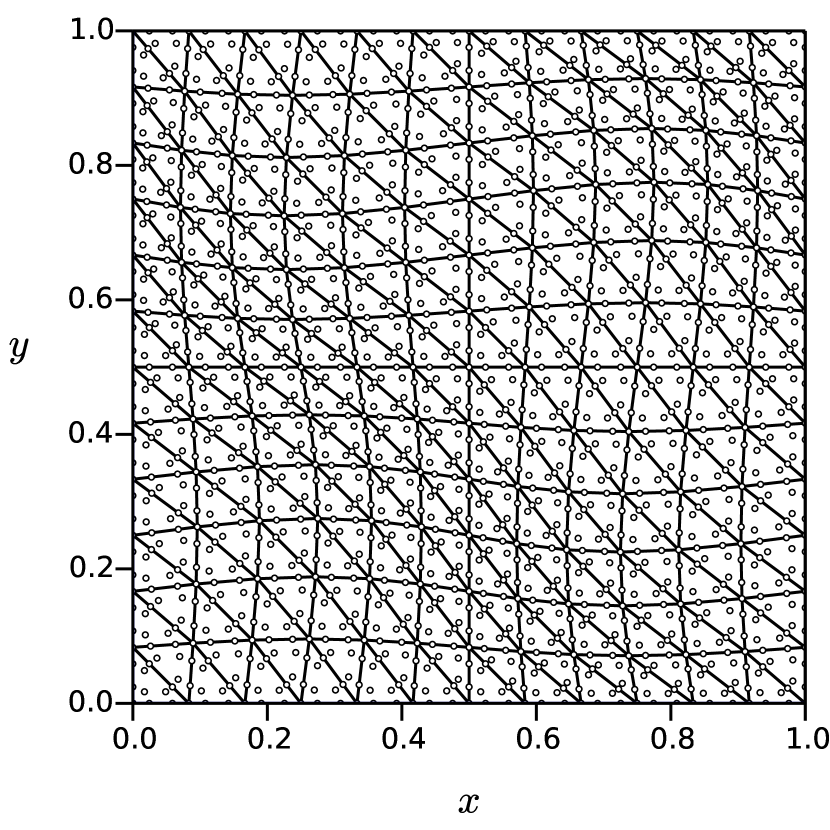
A nonuniform mesh for the square domain $\Omega$ is generated, in order to eliminate possible error cancellations that may arise on uniform grids. The vertices of the mesh are given by

$$x_{i,j}=\frac{i}{N}+\frac{1}{40}\sin\left(2\pi i/N\right)\sin\left(2\pi j/N\right),\qquad y_{i,j}=\frac{j}{N}+\frac{1}{40}\sin\left(2\pi i/N\right)\sin\left(2\pi j/N\right),$$

where $N$ is the number of elements along an edge, and $i,j=0,1,2,\ldots,N$. The nominal element size is $h\equiv 1/N$. A triangular mesh is generated by dividing each quadrilateral $\{x_{i,j},x_{i+1,j},x_{i,j+1},x_{i+1,j+1}\}$ along the diagonal from $x_{i+1,j}$ to $x_{i,j+1}$. Finally, for an SBP element of degree $p$, the reference-element nodes are mapped (affinely) to each triangle in the mesh. Figure 2 illustrates a representative mesh for $p=3$ and $N=12$.

Remark 5.

The use of an affine mapping on each element ensures that the mapping Jacobian is element-wise constant; consequently, the transformed PDE has constant coefficients in the reference space and the finite-difference operator remains SBP. More generally, curvilinear elements would require constructing SBP operators for each curved element.

We consider both continuous (C-SBP) and discontinuous (D-SBP) discretizations using the SBP operators. The global operators for the C-SBP discretization are constructed using the assembly process described in Section 4.5. In addition, the periodic boundaries are transparent to the global C-SBP operator, that is, nodes that coincide on the periodic boundary are considered the same. The D-SBP discretization of the surface fluxes follows the nodal DG method outlined, for example, in Hesthaven and Warburton [13, Chapter 6]. We use SATs with a penalty parameter of $\sigma=1$, which is equivalent to the use of upwind numerical flux functions.

The classical 4th-order Runge-Kutta scheme is used to discretize the time derivative. The maximally stable CFL number for each SBP operator was identified for $N=32$ using Golden-Section optimization, where the CFL number was defined as $\sqrt{2}\Delta t/(h\Delta r)=\sqrt{2}N\Delta t/\Delta r$ for a time-step size of $\Delta t$; $\Delta r$ denotes the minimum distance between nodes on a right triangle with vertices at $(0,0)$, $(1,0)$ and $(0,1)$. Each discretization was run for one period, $t\equiv T=1\;\textsf{unit}$, and considered stable if the final $L^{2}$ norm of the solution was less than or equal to the initial solution norm. The results of the optimization are listed in Table 1.

Table 1: Maximally stable CFL numbers for the SBP operators on the nonuniform mesh with $N=32$.

	p=1	p=2	p=3	p=4
C-SBP $\text{CFL}_{\max}$	1.885	2.257	1.816	1.570
D-SBP $\text{CFL}_{\max}$	0.696	1.269	1.157	1.148

5.1 Accuracy and efficiency studies

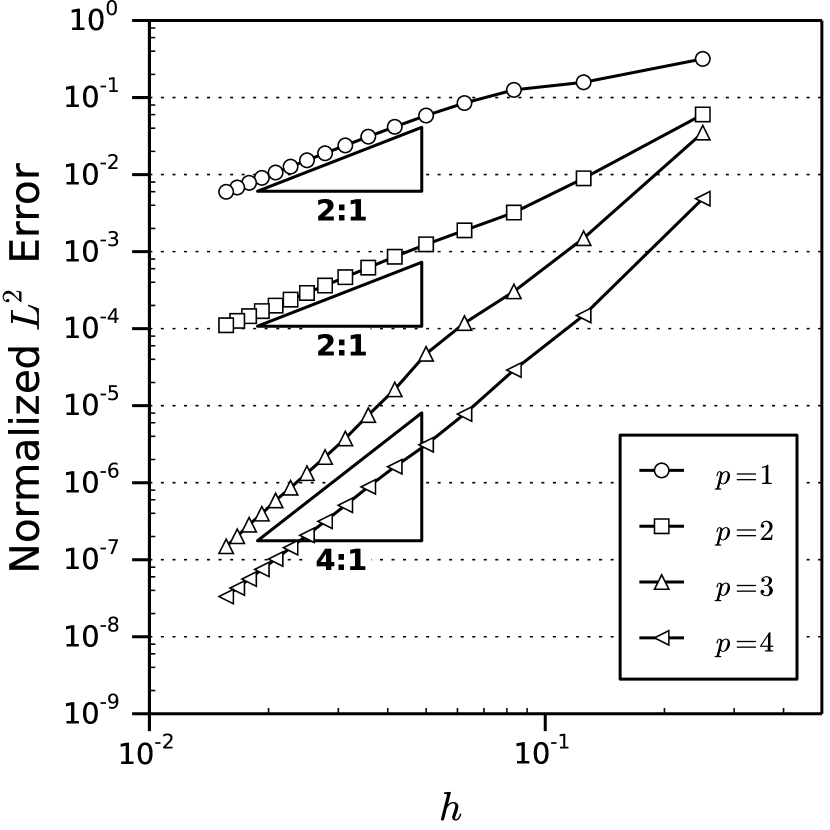
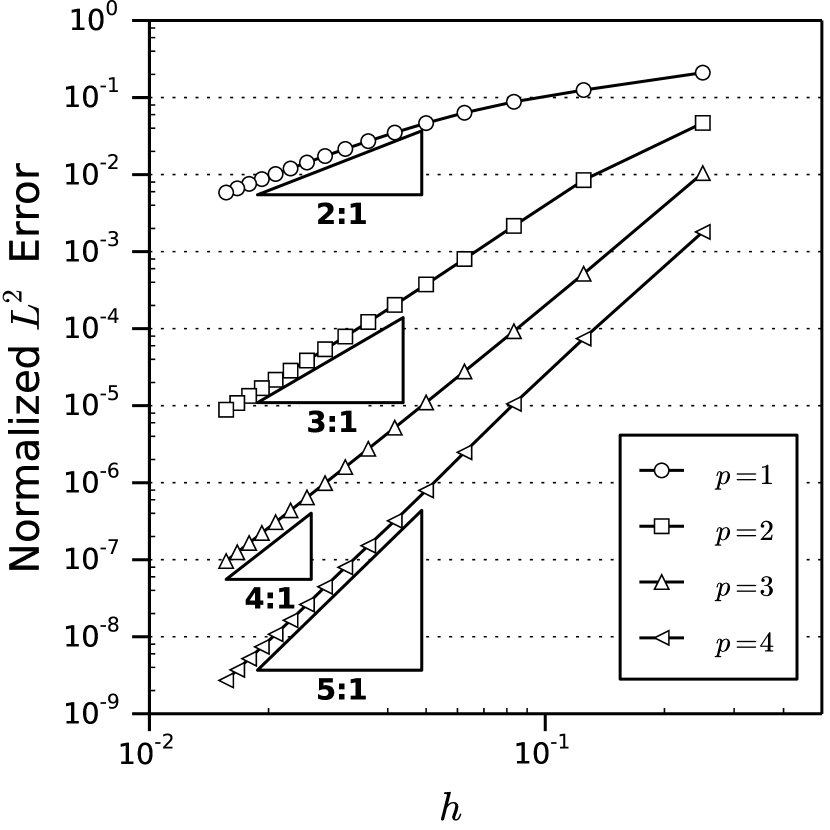
Figures 4 and 4 plot the normalized $L^{2}$ error for the C-SBP and D-SBP discretizations, respectively, for SBP-operator degrees one to four and a range of $N$. Specifically, if $\bm{u}_{0}$ is the initial solution, $\bm{u}$ is the solution at $t=T$, and $\mathsf{H}$ is the appropriate SBP norm, then the error is

$$L^{2}\;\mathsf{Error}=\sqrt{\left(\bm{u}-\bm{u}_{0}\right)^{\mathrm{T}}\mathsf{H}\left(\bm{u}-\bm{u}_{0}\right)}.$$

The error is normalized by the integral norm of the initial condition. The mesh resolution ranges from $N=4$ to $N=64$ in increments of 4. Each case was time marched using a CFL number of $0.9\text{CFL}_{\max}$, which was sufficiently small to produce negligible temporal discretization errors.

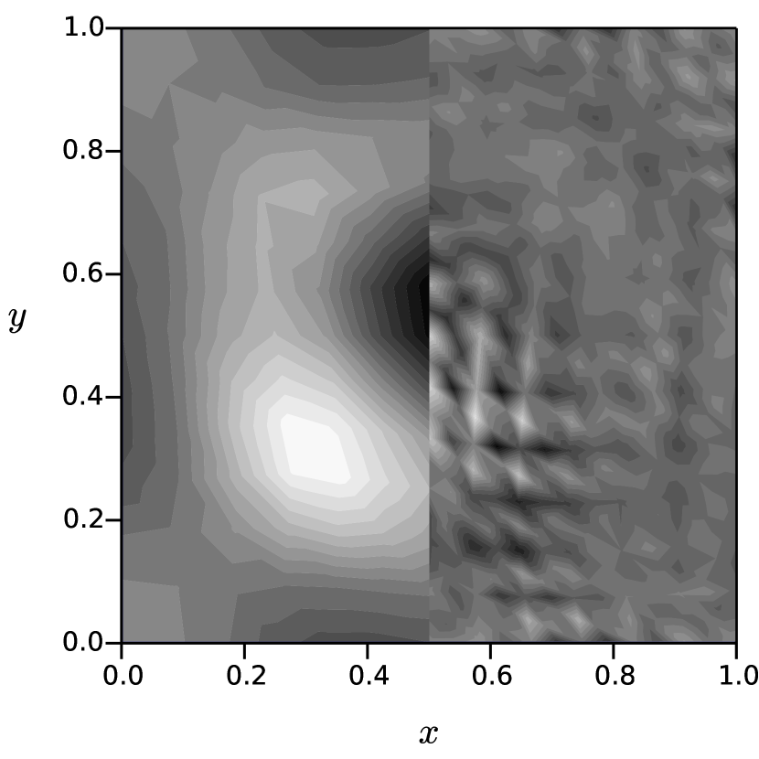
The results in Figure 4 indicate that the D-SBP discretizations and the odd-order C-SBP discretizations exhibit asymptotic convergence rates of $\text{O}(h^{p+1})$. In contrast, the C-SBP discretizations based on the $p=2$ and $p=4$ operators have convergence rates of $\text{O}(h^{p})$. These discretizations experience even-odd decoupling, i.e. checkerboarding, which is illustrated in Figure 2 by comparing the spatial error at $t=T$ for the $p=1$ and $p=2$ C-SBP discretizations; the $p=1$ error is smooth whereas the $p=2$ error is oscillatory. Checkerboarding is not unique to the SBP simplex operators, and can be observed with one-dimensional SBP operators. We are currently investigating methods to address this issue with the even-order C-SBP discretizations.

Fig. 1: Example mesh with $p=3$ and $N=12$ for accuracy and energy-norm studies.

Fig. 2: Solution error after one period, $t=T$, for the $p=1$ (left) and $p=2$ (right) C-SBP discretizations with $N=12$.

Fig. 3: $L^{2}$ error between the C-SBP solution after one period, $t=T$, and the initial condition for different mesh spacing and operators.

Fig. 4: $L^{2}$ error between the D-SBP solution after one perior, $t=T$, and the initial condition for different mesh spacing and operators.

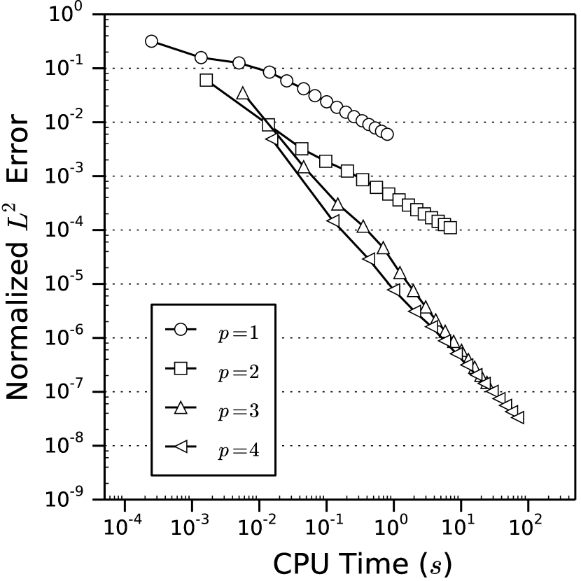
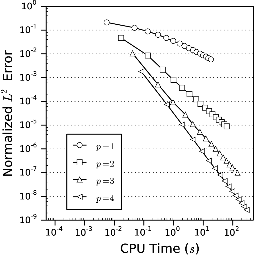
Figures 6 and 6 plot the normalized $L^{2}$ error versus CPU time for both the C-SBP and D-SBP discretizations. The runs were performed on an Intel^® Core i5-3570K processor, and the code was implemented in Julia version 0.4.0. The efficiency provided by the high-order operators is apparent in both the continuous and discontinuous cases.

Fig. 5: Normalized $L^{2}$ error of the C-SBP solutions after one period versus CPU time measured in seconds.

Fig. 6: Normalized $L^{2}$ error of the D-SBP solutions after one period versus CPU time measured in seconds.

5.2 Stability studies

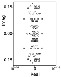
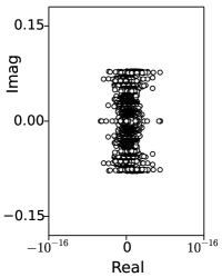
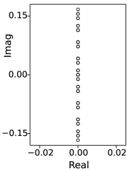
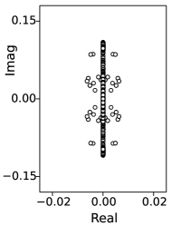
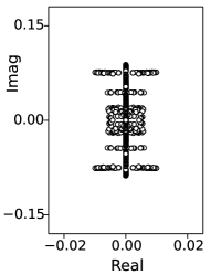
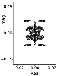
Figure 7 shows the spectra of the C-SBP and SE spatial discretizations for the linear advection problem. Specifically, these eigenvalues are for the global operator $\mathsf{S}_{x}+\mathsf{S}_{y}$ when $N=12$. The eigenvalues of the C-SBP operators are imaginary to machine precision, which mimics the continuous spectrum for this periodic problem. This is as expected, because the boundary operators $\mathsf{E}_{x}^{(k)}$ cancel between adjacent elements when the SBP derivative operator is assembled, leaving only the antisymmetric parts. The SE operator for $p=1$ also has a purely imaginary spectrum, because it is identical to the linear SBP operator; however, the spectra of the high-order SE operators have a real component.

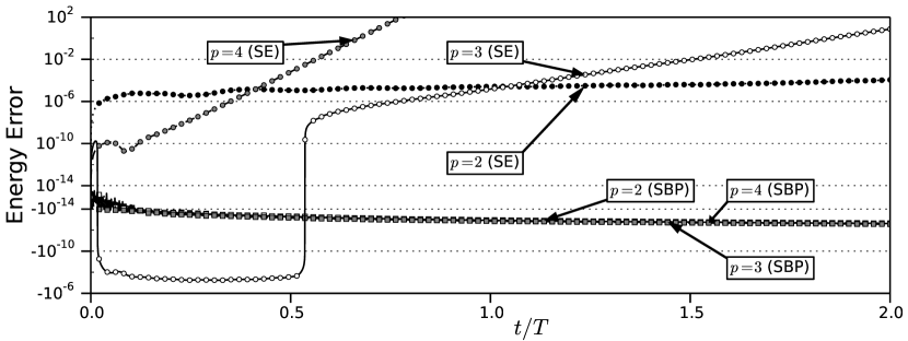
The consequences of the eigenvalue distributions are evident when the linear advection problem is integrated for two periods. Figure 8 plots the difference between the solution $L^{2}$ norm at time $t\in[0,2]$ and the initial solution norm, i.e. the change in “energy”,

$$\Delta E=\bm{u}_{n}^{\mathrm{T}}\mathsf{H}\bm{u}_{n}-\bm{u}_{0}^{\mathrm{T}}\mathsf{H}\bm{u}_{0},$$

where $\bm{u}_{n}$ denotes the discrete solution at time step $n$. For this study, $N=12$ and the CFL number was fixed at 0.01 to reduce temporal errors.

The energy history in Figure 8 clearly shows that the SE operators are unstable for this linear advection problem, while the SBP operators are stable. The small (linear) decrease in the SBP energy error is due to temporal errors and can be eliminated by using a different time-marching method, e.g. leapfrog, or at the cost of using a sufficiently small CFL number.

$p=1$ (SBP)

$p=2$ (SBP)

$p=3$ (SBP)

$p=4$ (SBP)

$p=1$ (SE)

$p=2$ (SE)

$p=3$ (SE)

$p=4$ (SE)

Fig. 7: Eigenvalue distributions for the SBP (upper row) and the SE (lower row) spatial discretizations of the linear advection problem. Note the different ranges for the real axes.

Fig. 8: Time history of the change in the solution energy norm. Note the use of a symmetric logarithmic scale on the vertical axis.

6 Conclusions

We proposed a definition for multi-dimensional SBP operators that is a natural extension of one-dimensional SBP definitions. We studied the theoretical implications of the definition in the case of diagonal-norm operators, and showed that the multi-dimensional operators retain the attractive properties of tensor-product SBP operators. A significant theoretical result of this work is that, for a given domain, a cubature rule with positive weights and a full-rank Vandermonde matrix (evaluated at the cubature nodes) are necessary and sufficient for the existence of diagonal-norm SBP operators on that domain. We also developed simultaneous approximation terms (SATs) for the weak imposition of boundary conditions, and we showed that an SBP-SAT discretization of the linear advection equation is time stable.

We constructed diagonal-norm SBP operators for the triangle and tetrahedron. To the best of our knowledge, this is the first example of SBP operators of degree $p\geq 2$ on these domains. We also presented an assembly procedure that constructs SBP operators for a global domain from element-wise SBP operators.

Finally, we verified the triangle-element SBP operators using both continuous and discontinuous (i.e. SAT) inter-element coupling. Results for linear advection on a doubly periodic domain demonstrated the time stability and accuracy of the SBP discretizations. The results suggest that the proposed operators could be effective for the long-time simulation of turbulent flows on complex domains.

Appendix A Decomposition of the SAT matrix $\beta_{x}\mathsf{E}_{x}+\beta_{y}\mathsf{E}_{y}$

Let $\mathsf{E}\equiv\beta_{x}\mathsf{E}_{x}+\beta_{y}\mathsf{E}_{y}$. Recall the block-matrix definition of $\mathsf{E}_{x}$ used in the proof of Theorem 4. Using that definition, and a similar definition for $\mathsf{E}_{y}$, we have

$$\tilde{\mathsf{V}}^{-\mathrm{T}}\mathsf{E}\tilde{\mathsf{V}}^{-1}=\tilde{\mathsf{V}}^{-\mathrm{T}}\begin{bmatrix}\tilde{\mathsf{E}}&\mathsf{F}^{T}\\ \mathsf{F}&\mathsf{G}\end{bmatrix}\tilde{\mathsf{V}}^{-1}\equiv\beta_{x}\tilde{\mathsf{V}}^{-\mathrm{T}}\begin{bmatrix}\tilde{\mathsf{E}}_{x}&\mathsf{F}_{x}^{\mathrm{T}}\\ \mathsf{F}_{x}&\mathsf{G}_{x}\end{bmatrix}\tilde{\mathsf{V}}^{-1}+\beta_{y}\tilde{\mathsf{V}}^{-\mathrm{T}}\begin{bmatrix}\tilde{\mathsf{E}}_{y}&\mathsf{F}_{y}^{\mathrm{T}}\\ \mathsf{F}_{y}&\mathsf{G}_{y}\end{bmatrix}\tilde{\mathsf{V}}^{-1}.$$

From the definition of $\tilde{\mathsf{E}}_{x}$ and $\tilde{\mathsf{E}}_{y}$, we have that the entries in the block $\tilde{\mathsf{E}}$ are given by

$$\left(\tilde{\mathsf{E}}\right)_{k,m}=\oint_{\Gamma}\mathcal{P}_{k}(x,y)\mathcal{P}_{m}(x,y)\left(\beta_{x}n_{x}+\beta_{y}n_{y}\right)\mathrm{d}\Gamma\qquad\forall\;k,m\in\{1,\dots,n^{*}_{\tau}\},$$

where $\mathcal{P}_{k}$ and $\mathcal{P}_{l}$ have total degrees less than or equal to $\tau$. We can decompose $\tilde{\mathsf{E}}$ by breaking the above integral into two integrals, one over $\Gamma_{+}$ and one over $\Gamma_{-}$:

$$\left(\tilde{\mathsf{E}}\right)_{k,m}=\oint_{\Gamma_{+}}\mathcal{P}_{k}\mathcal{P}_{m}\left(\beta_{x}n_{x}+\beta_{y}n_{y}\right)\mathrm{d}\Gamma+\oint_{\Gamma_{-}}\mathcal{P}_{k}\mathcal{P}_{m}\left(\beta_{x}n_{x}+\beta_{y}n_{y}\right)\mathrm{d}\Gamma=\tilde{\mathsf{E}}_{+}+\tilde{\mathsf{E}}_{-},\\ \forall\;k,m\in\{1,\dots,n^{*}_{\tau}\}.$$

where $\tilde{\mathsf{E}}_{+}$ and $\tilde{\mathsf{E}}_{-}$ are equated with the integrals over $\Gamma_{+}$ and $\Gamma_{-}$, respectively.

Lemma 8.

The matrix $\tilde{\mathsf{E}}_{-}$ is negative semi-definite and the matrix $\tilde{\mathsf{E}}_{+}$ is positive semi-definite.

Proof.

We prove the result for $\tilde{\mathsf{E}}_{-}$, since the proof for the positive-definite matrix is analogous. Let $\bm{u}\in\mathbb{R}^{n^{*}_{p}}$ be an arbitrary nonzero vector, and let $u_{k}$ denote its entries. Then

$$\bm{u}^{T}\tilde{\mathsf{E}}_{-}\bm{u} =\sum_{k=1}^{n^{*}_{\tau}}\sum_{l=1}^{n^{*}_{\tau}}\oint_{\Gamma_{-}}\left(u_{k}\mathcal{P}_{k}(x,y)\right)\left(u_{l}\mathcal{P}_{l}(x,y)\right)\left(\beta_{x}n_{x}+\beta_{y}n_{y}\right)\mathrm{d}\Gamma$$

$$=\oint_{\Gamma_{-}}\left[\mathcal{U}(x,y)\right]^{2}\left(\beta_{x}n_{x}+\beta_{y}n_{y}\right)\mathrm{d}\Gamma$$

where $\mathcal{U}(x,y)\equiv\sum_{k=1}^{n^{*}_{\tau}}u_{k}\mathcal{P}_{k}(x,y)$. The integrand in the above is the product of a squared polynomial function and the non-positive quantity $(\beta_{x}n_{x}+\beta_{y}n_{y})\leq 0$ $\forall\;(x,y)\in\Gamma_{-}$. Thus the desired result follows.   ∎

We now turn to the main result of this appendix:

Theorem 9.

Suppose $\mathsf{F}_{x}=\mathsf{0}$ and $\mathsf{F}_{y}=\mathsf{0}$ in the definitions of $\mathsf{E}_{x}$ and $\mathsf{E}_{y}$. Then, for any $\beta_{x},\beta_{y}\in\mathbb{R}$, the matrix $\mathsf{E}\equiv\beta_{x}\mathsf{E}_{x}+\beta_{y}\mathsf{E}_{y}$ can be decomposed into $\mathsf{E}=\mathsf{E}_{+}+\mathsf{E}_{-}$ where $\mathsf{E}_{+}$ is positive semi-definite, $\mathsf{E}_{-}$ is negative semi-definite, and $\mathsf{E}_{\pm}$ satisfy the accuracy conditions

$$\bm{p}_{k}^{\mathrm{T}}\mathsf{E}_{\pm}\bm{p}_{m}=\displaystyle\oint_{\Gamma_{\pm}}\mathcal{P}_{k}\mathcal{P}_{m}\left(\beta_{x}n_{x}+\beta_{y}n_{y}\right)\mathrm{d}\Gamma,\qquad\forall\;k,m\in\{1,2,\dots,n^{*}_{\tau}\}.$$ (14)

Proof.

Consider the decomposition

$$\mathsf{E}=\mathsf{E}_{+}+\mathsf{E}_{-}=\tilde{\mathsf{V}}^{-\mathrm{T}}\begin{bmatrix}\tilde{\mathsf{E}}_{+}&\left(\mathsf{F}_{+}\right)^{\mathrm{T}}\\ \mathsf{F}_{+}&\mathsf{G}_{+}\end{bmatrix}\tilde{\mathsf{V}}^{-1}+\tilde{\mathsf{V}}^{-\mathrm{T}}\begin{bmatrix}\tilde{\mathsf{E}}_{-}&\left(\mathsf{F}_{-}\right)^{\mathrm{T}}\\ \mathsf{F}_{-}&\mathsf{G}_{-},\end{bmatrix}\tilde{\mathsf{V}}^{-1},$$

where $\tilde{\mathsf{E}}_{\pm}$ are defined above, and the pairs $(\mathsf{F}_{+},\mathsf{F}_{-})$ and $(\mathsf{G}_{+},\mathsf{G}_{-})$ are yet-to-be-determined decompositions of $\beta_{x}\mathsf{F}_{x}+\beta_{y}\mathsf{F}_{y}$ and $\beta_{x}\mathsf{G}_{x}+\beta_{y}\mathsf{G}_{y}$, respectively; note that the above decomposition of $\mathsf{E}$ is distinct from its definition, which involves $\mathsf{E}_{x}$ and $\mathsf{E}_{y}$.

The accuracy of the matrices $\mathsf{E}_{+}$ and $\mathsf{E}_{-}$, as defined above, can be established using the same approach used in the proof of Theorem 4. Therefore, we focus on showing that $\mathsf{E}_{-}$ can be made negative semi-definite; again, an analogous proof can be used to show $\mathsf{E}_{+}$ is positive semi-definite.

To prove that $\mathsf{E}_{-}$ is negative semi-definite, it suffices to show that the matrix

$$\begin{bmatrix}\tilde{\mathsf{E}}_{-}&\left(\mathsf{F}_{-}\right)^{\mathrm{T}}\\ \mathsf{F}_{-}&\mathsf{G}_{-}\end{bmatrix}$$

is negative semi-definite. This will be the case if we can ensure $\mathsf{G}_{-}$ is negative-definite and the corresponding Schur complement,

$$\mathsf{S}_{-}\equiv\tilde{\mathsf{E}}_{-}-\left(\mathsf{F}_{-}\right)^{\mathrm{T}}\left(\mathsf{G}_{-}\right)^{-1}\mathsf{F}_{-},$$

is negative semi-definite; see, for example, [1, Appendix A.5.5].

We first tackle the definiteness of $\mathsf{G}_{-}$. Recall that $\mathsf{G}_{x}$ and $\mathsf{G}_{y}$ are symmetric but otherwise arbitrary. Therefore, the matrix $\mathsf{G}=\beta_{x}\mathsf{G}_{x}+\beta_{y}\mathsf{G}_{y}$ has the eigendecomposition $\mathsf{G}=\mathsf{R}\Lambda\mathsf{R}^{\mathrm{T}}$, where $\mathsf{R}$ holds the eigenvectors and the diagonal matrix $\Lambda$ holds the eigenvalues. For any set of eigenvalues, we can construct the nonunique decomposition

$$\mathsf{G}=\mathsf{R}\Lambda_{+}\mathsf{R}^{\mathrm{T}}+\mathsf{R}\Lambda_{-}\mathsf{R}^{\mathrm{T}},$$

such that $\Lambda_{+}$ is diagonal positive-definite and $\Lambda_{-}$ is diagonal negative-definite; note that any zero eigenvalue in $\Lambda$ can be decomposed as $c-c$ for arbitrary $c>0$. Equating $\mathsf{G}_{-}$ with $\mathsf{R}\Lambda_{-}\mathsf{R}^{\mathrm{T}}$ we have that $\mathsf{G}_{-}$ is symmetric negative-definite and therefore invertible.

Finally, we need to show that $\mathsf{S}_{-}$ is negative semi-definite. From Lemma 8, we have that $\tilde{\mathsf{E}}_{-}$ is negative semi-definite. Thus, showing $\mathsf{S}_{-}\preceq\mathsf{0}$ is equivalent to showing

$$\tilde{\mathsf{E}}_{-}\preceq\left(\mathsf{F}_{-}\right)^{\mathrm{T}}\left(\mathsf{G}_{-}\right)^{-1}\mathsf{F}_{-},$$

This statement is true provided the entries in $\mathsf{F}_{-}$ are sufficiently small, which is certainly the case under the assumption that $\mathsf{F}_{x}=\mathsf{F}_{y}=\mathsf{0}$. This concludes the proof.   ∎

Remark 6.

In general, the assumption that $\mathsf{F}_{x}=\mathsf{F}_{y}=\mathsf{0}$ is stronger than necessary, since only $\mathsf{S}_{-}\preceq 0$ is required; however, it is not clear how to weaken this assumption when $\beta_{x}$ and $\beta_{y}$ are not known a priori.

Remark 7.

The matrices $\mathsf{E}_{x}$ and $\mathsf{E}_{y}$ constructed for the simplex operators satisfy the conditions of the Theorem 9, i.e. $\mathsf{F}_{x}=\mathsf{F}_{y}=\mathsf{0}$.

References

- [1] Stephen Boyd and Lieven Vandenberghe, Convex Optimization, Cambridge University Press, Mar. 2004.
- [2] Mark H. Carpenter and David Gottlieb, Spectral methods on arbitrary grids, Journal of Computational Physics, 129 (1996), pp. 74–86.
- [3] Mark H. Carpenter, David Gottlieb, and Saul Abarbanel, Time-stable boundary conditions for finite-difference schemes solving hyperbolic systems: Methodology and application to high-order compact schemes, Journal of Computational Physics, 111 (1994), pp. 220–236.
- [4] Mark H. Carpenter, Jan Nordström, and David Gottlieb, A stable and conservative interface treatment of arbitrary spatial accuracy, Journal of Computational Physics, 148 (1999), pp. 341–365.
- [5] Edmond K. Chiu, Qiqi Wang, and Antony Jameson, A conservative meshless scheme: general order formulation and application to Euler equations, in 49th AIAA Aerospace Sciences Meeting, no. AIAA–2011–651, Orlando, Florida, Jan. 2011.
- [6] Gary Cohen, Patrick Joly, Jean E. Roberts, and Nathalie Tordjman, Higher order triangular finite elements with mass lumping for the wave equation, SIAM Journal on Numerical Analysis, 38 (2001), pp. 2047–2078.
- [7] David C. Del Rey Fernández, Pieter D. Boom, and David W. Zingg, A generalized framework for nodal first derivative summation-by-parts operators, Journal of Computational Physics, 266 (2014), pp. 214–239.
- [8] Moshe Dubiner, Spectral methods on triangles and other domains, Journal of Scientific Computing, 6 (1991), pp. 345–390.
- [9] Daniele Funaro and David Gottlieb, A new method of imposing boundary conditions in pseudospectral approximations of hyperbolic equations, Mathematics of Computation, 51 (1988), pp. 599–613.
- [10] Gregor J. Gassner, A skew-symmetric discontinuous Galerkin spectral element discretization and its relation to sbp-sat finite difference methods, SIAm Journal on Scientific Computing, 35 (2013), pp. A1233–A1253.
- [11] Francis X. Giraldo and Mark A. Taylor, A diagonal-mass-matrix triangular-spectral-element method based on cubature points, Journal of Engineering Mathematics, 56 (2006), pp. 307–322.
- [12] Gene H. Golub and Charles F. Van Loan, Matrix Computations, The John Hopkins University Press, third ed., 1996.
- [13] Jan S. Hesthaven and Tim Warburton, Nodal discontinuous Galerkin methods: algorithms, analysis, and applications, Springer-Verlag, New York, 2008.
- [14] Jason E. Hicken and David W. Zingg, A parallel Newton-Krylov solver for the Euler equations discretized using simultaneous approximation terms, AIAA Journal, 46 (2008), pp. 2773–2786.
- [15] Jason E. Hicken and David W. Zingg, Summation-by-parts operators and high-order quadrature, Journal of Computational and Applied Mathematics, 237 (2013), pp. 111–125.
- [16] John D. Hunter, Matplotlib: A 2D graphics environment, Computing In Science & Engineering, 9 (2007), pp. 90–95.
- [17] Adrian Kitson, Robert I. McLachlan, and Nicolas Robidoux, Skew-adjoint finite difference methods on nonuniform grids, New Zealand Journal of Mathematics, 32 (2003), pp. 139–159.
- [18] Tom Koornwinder, Two-variable analogues of the classical orthogonal polynomials, in Theory and application of special functions, Academic Press New York, 1975, pp. 435–495.
- [19] Heinz-Otto Kreiss and Godela Scherer, Finite element and finite difference methods for hyperbolic partial differential equations, in Mathematical aspects of finite elements in partial differential equations, Academic Press, New York/London, 1974, pp. 195–212.
- [20] Edmond Kwan-yu Chiu, Qiqi Wang, Rui Hu, and Antony Jameson, A conservative Mesh-Free scheme and generalized framework for conservation laws, SIAM Journal on Scientific Computing, 34 (2012), pp. A2896–A2916.
- [21] Yen Liu and Marcel Vinokur, Exact integrations of polynomials and symmetric quadrature formulas over arbitrary polyhedral grids, Journal of Computational Physics, 140 (1998), pp. 122–147.
- [22] Yen Liu, Marcel Vinokur, and Z. J. Wang, Spectral difference method for unstructured grids i: Basic formulation, Journal of Computational Physics, 216 (2006), pp. 780–801.
- [23] Ken Mattsson, Summation by Parts Operators for Finite Difference Approximations of Second-Derivatives with Variable Coefficients, Journal of Scientific Computing, 51 (2012), pp. 650–682.
- [24] Ken Mattsson and Jan Nordström, Summation by parts operators for finite difference approximations of second derivatives, Journal of Computational Physics, 199 (2004), pp. 503–540.
- [25] Yohei Morinishi, Thomas S. Lund, Oleg V. Vasilyev, and Parviz Moin, Fully Conservative Higher Order Finite Difference Schemes for Incompressible Flow, Journal of Computational Physics, 143 (1998), pp. 90–124.
- [26] Wim A. Mulder, Higher-order mass-lumped finite elements for the wave equation, Journal of Computational Acoustics, 09 (2001), pp. 671–680.
- [27] Jan Nordström, Conservative finite difference formulations, variable coefficients, energy estimates and artificial dissipation, Journal of Scientific Computing, 29 (2006), pp. 375–404.
- [28] Jan Nordström, Karl Forsberg, Carl Adamsson, and Peter Eliasson, Finite volume methods, unstructured meshes and strict stability for hyperbolic problems, Applied Numerical Mathematics, 45 (2003), pp. 453–473.
- [29] Jan Nordström, Jing Gong, Edwin van der Weide, and Magnus Svärd, A stable and conservative high order multi-block method for the compressible Navier-Stokes equations, Journal of Computational Physics, 228 (2009), pp. 9020–9035.
- [30] Bo Strand, Summation by parts for finite difference approximations for d/dx, Journal of Computational Physics, 110 (1994), pp. 47–67.
- [31] Magnus Svärd, On coordinate transformations for summation-by-parts operators, Journal of Scientific Computing, 20 (2004), pp. 29–42.
- [32] Magnus Svärd, Ken Mattsson, and Jan Nordström, Steady-State computations using Summation-by-Parts operators, Journal of Scientific Computing, 24 (2005), pp. 79–95.
- [33] Freddie D. Witherden and Pieter Vincent, On the identification of symmetric quadrature rules for finite element methods, Sept. 2014.
- [34] Helen C. Yee and Björn Sjögreen, Designing adaptive low-dissipative high order schemes for long-time integrations, in Turbulent Flow Computation, Springer, 2002, pp. 141–198.
- [35] Helen C. Yee, Marcel Vinokur, and M. Jahed Djomehri, Entropy splitting and numerical dissipation, Journal of Computational Physics, 162 (2000), pp. 33–81.
- [36] Linbo Zhang, Tao Cui, and Hui Liu, A set of symmetric quadrature rules on triangles and tetrahedra, Journal of Computational Mathematics, 27 (2009), pp. 89–96.