Quaternionic R transform and non-hermitian random matrices

Zdzislaw Burda zdzislaw.burda@agh.edu.pl Faculty of Physics and Applied Computer Science, AGH University of Science and Technology, al. Mickiewicza 30, PL–30059 Kraków, Poland    Artur Swiech swiech@thp.uni-koeln.de Institute for Theoretical Physics,
University of Cologne, Zülpicher Straße 77, D-50937 Köln, Germany
Abstract

Using the Cayley-Dickson construction we rephrase and review the non-hermitian diagrammatic formalism [R. A. Janik, M. A. Nowak, G. Papp and I. Zahed, Nucl.Phys. B 501, 603 (1997)], that generalizes the free probability calculus to asymptotically large non-hermitian random matrices. The main object in this generalization is a quaternionic extension of the R transform which is a generating function for planar (non-crossing) cumulants. We demonstrate that the quaternionic R transform generates all connected averages of all distinct powers of X𝑋X and its hermitian conjugate Xsuperscript𝑋X^{\dagger}: 1NTrXaXbXcdelimited-⟨⟩delimited-⟨⟩1𝑁Trsuperscript𝑋𝑎superscript𝑋absent𝑏superscript𝑋𝑐\langle\langle\frac{1}{N}\mbox{Tr}X^{a}X^{\dagger b}X^{c}\ldots\rangle\rangle for N𝑁N\rightarrow\infty. We show that the R transform for gaussian elliptic laws is given by a simple linear quaternionic map (z+wj)=x+σ2(μe2iϕz+wj)𝑧𝑤𝑗𝑥superscript𝜎2𝜇superscript𝑒2𝑖italic-ϕ𝑧𝑤𝑗\mathcal{R}(z+wj)=x+\sigma^{2}\left(\mu e^{2i\phi}z+wj\right) where (z,w)𝑧𝑤(z,w) is the Cayley-Dickson pair of complex numbers forming a quaternion q=(z,w)z+wj𝑞𝑧𝑤𝑧𝑤𝑗q=(z,w)\equiv z+wj. This map has five real parameters ex𝑒𝑥\Re ex, mx𝑚𝑥\Im mx, ϕitalic-ϕ\phi, σ𝜎\sigma and μ𝜇\mu. We use the R transform to calculate the limiting eigenvalue densities of several products of gaussian random matrices.

random matrix theory, non-hermitian, free probability
pacs:
02.50.Cw (Probability theory), 02.70.Uu (Applications of Monte Carlo methods)

I Introduction

Random matrices play an important role in physics, engineering and mathematics m ; cpv ; ckn ; gmw ; abf ; vt ; agz . While dealing with random matrices one often faces the problem of calculating eigenvalue spectra of sums and products of random matrices. This problem can be partially solved in the case of infinite invariant random matrices using methods of free probability which is a powerful technique developed recently v1 ; v2 ; vdn ; s . In practice, with some caution, one can use free probability results also as a good approximation for finite (large) matrices.

Free probability calculus was introduced in operator algebra v1 ; v2 . Later one has realized that it can be also applied to random matrices in calculations of moments of sums and products of large invariant hermitian random matrices s . In short, using free probability one can express the moment generating functions for a sum A+B𝐴𝐵A+B or a product AB𝐴𝐵AB of invariant random matrices A𝐴A and B𝐵B in terms of the moment generating functions of these matrices. If a random matrix is hermitian the knowledge of its moments is often sufficient to reconstruct its eigenvalue density. Unfortunately the product P=AB𝑃𝐴𝐵P=AB, even for hermitian matrices, is generically non-hermitian. To get around this problem some authors rs consider a related hermitian random matrix P=ABAsuperscript𝑃𝐴𝐵𝐴P^{\prime}=\sqrt{A}B\sqrt{A}, which has identical moments as P𝑃P: TrPk=TrPkTrsuperscript𝑃𝑘Trsuperscript𝑃𝑘\mathrm{Tr}P^{\prime k}=\mathrm{Tr}P^{k}. Unfortunately the eigenvalue density of Psuperscript𝑃P^{\prime}, except for a special class of matrices, is not the same as of P𝑃P. So if one is interested in the eigenvalue density of P𝑃P one has to either apply different methods bjw ; ab or to extend free probability calculus to the realm of non-hermitian matrices. For example, one might be interested in the eigenvalue density of the product of two independent GUE matrices. Clearly, the product is a non-hermitian matrix, its eigenvalues are complex and the eigenvalue density has a non-trivial support. Actually one can find the limiting eigenvalue density of this product to be ρ(z)=(2π|z|)1𝜌𝑧superscript2𝜋𝑧1\rho(z)=(2\pi|z|)^{-1} on the unit disk and zero outside the disk bjw ; ab .

Non-hermitian random matrices have been studied in many contexts, including chaotic scattering hil ; fs1 ; fs2 ; fss , quantum chromodynamics with chemical potential jnz ; v , networks scss ; dki , lagged correlations bt ; j , matrix-valued random walk gjjn ; bgntw and many others ra ; sg . As a result of these intensive studies one has developed analytic techniques to calculate the eigenvalue spectra of such matrices. In the heart of these techniques lies an electrostatic analogy scss ; fs2 . In this analogy eigenvalues of the random matrix play the role of positions of electric charges on two-dimensional plane and the Green’s function of electric field. Given the Green’s function one can calculate the eigenvalue density from the Gauss law scss ; fs2 ; rj ; jnpz1 . The Green’s function can be viewed as an subordinated element of a two-by-two matrix being an extended Green’s function. There were two independent approaches proposed for this extension: the first one was directly derived rj ; jnpz1 ; jnpz2 ; jnpwz from the regularization of the electrostatic potential scss ; fs2 ; hil and the other one was obtained by a method of hermitization fz1 ; fz2 . Both the constructions are equivalent to each other and both can be formulated in terms of quaternions as one can see from the today’s perspective.

The quaternionic nature of these equations was anticipated in fz1 and worked out in jn1 ; jn2 where a very deep geometrical understanding of the regularization procedure was achieved. More precisely, in the calculations one usually introduces a regulator ϵitalic-ϵ\epsilon. The modulus |ϵ|italic-ϵ|\epsilon| can be interpreted as a distance from the complex plane. This means that calculations are in fact performed in the quaternionic space in the neighborhood of the complex plane and only towards the end of the calculations, when the limit ϵ0italic-ϵ0\epsilon\rightarrow 0 is taken, the problem is projected back to the complex plane. The idea is similar to that used in the Sokhotski’s formula (4) for one-dimensional delta function on the real axis except that now it is applied to two-dimensional delta function on the complex plane. In order to exploit this similarity it is convenient to recall the Cayley-Dickson construction. In this construction complex numbers are defined as pairs of real numbers and quaternions as pairs of complex numbers. In the one-dimensional Sokhotski’s formula one sends the second element of the Cayley-Dickson pair (imaginary part) to zero ϵ0italic-ϵ0\epsilon\rightarrow 0 and regains one-dimensional delta function on the real axis while for the two-dimensional case one sends the second element of the Cayley-Dickson pair forming quaternion to zero and recovers the delta function on the complex plane fz1 ; jn1 ; jn2 .

Yet before the importance of the underlying quaternionic structure of the extended resolvents was recognized jn1 ; jn2 one was able to derive the corresponding extended R transform (or equivalent blue function, sometimes used in physical literature) and to formulate the addition law for non-hermitian matrices rj ; jnpz1 ; jnpz2 ; jnpwz ; fz1 . This law was then successfully applied to a number of problems, while the multiplication law for non-hermitian matrices was formulated much later bjn .

Although quaternionic picture emerged already a decade ago fz1 ; jn1 ; jn2 and has been applied to various problems bgntw ; r ; bcc ; j2 , it has not been commonly adopted. The reason for this is probably related to the fact, that the synthetic picture of what is the R transform for non-hermitian matrices was still missing. It was not clear how the R transform was related to the moments of the random matrix or what was the classification of the R transform in the simplest case of gaussian laws, etc. We fill up this gap here.

We show that the quaternionic structure of the resolvent and the R transform is capable to incorporate all mixed moments of random matrix and its hermitian conjugate: 1NTrXaXbXcdelimited-⟨⟩1𝑁Trsuperscript𝑋𝑎superscript𝑋absent𝑏superscript𝑋𝑐\langle\frac{1}{N}\mbox{Tr}X^{a}X^{\dagger b}X^{c}\ldots\rangle, for an asymptotic class of random matrix models define by the probability measure of the type (44) for N𝑁N\rightarrow\infty. In contrast to hermitian case, though, these moments cannot be constructed from the moments of the eigenvalue density ρ(λ)𝜌𝜆\rho(\lambda) as they also depend on the left and right eigenvector correlations of the matrix X𝑋X cm ; jnnpz . So in a sense, the Green’s function and the R transform encode also information about the eigenvector correlations.

The link between free probability and random matrices was established through planar combinatorics s . In fact, the relation of random matrices to planar combinatorics was discovered long before free probability, by gaussian perturbation theory of invariant matrix models, which maps the problem of calculating moments of random matrices to enumeration of planar Feynman diagrams th ; bipz . Planar Feynman diagrams can be enumerated by field theoretical methods, in particular by Dyson-Schwinger equations, which relate various moment generating functions bipz ; biz . These equations are very powerful, as one can use them to derive all relations between generating functions known from free probability. The idea is very universal and it can be also applied to non-hermitian matrices to derive relations between the quaternionic R transforms for independent random matrices A𝐴A, B𝐵B and the corresponding sums A+B𝐴𝐵A+B rj ; jnpz1 ; jnpz2 ; jnpwz and products AB𝐴𝐵AB bjn . We follow this approach here.

While presenting the material we first recall the hermitian case, which is well known and directly linked to free probability, and then we use it as a reference point while showing construction of the corresponding objects for non-hermitian matrices. We begin with the Green’s function and then turn to the R transform. Once we have recalled the definition of R transform for the non-hermitian matrices jn1 ; jn2 , we will classify all possible forms of this transform for gaussian elliptic ensembles gi . Then we extend the discussion to non-gaussian invariant measures (44) and link them to planar Feynman diagrams bipz ; biz . We recall the addition law rj ; jnpz1 ; jnpz2 ; jnpwz and the multiplication law for non-hermitian matrices bjn and use them to evaluate eigenvalue density for a couple of examples of products of gaussian random matrices from elliptic ensembles. We shortly summarize the paper in the last section. In Appendix A we recall the Cayley-Dickson construction of quaternions. In Appendix B we discuss quaternionic representation of the two-dimensional delta function, in Appendix C we recall the corresponding representation of the sum of delta functions located at the eigenvalues of a given non-hermitian matrix fs2 and finally in Appendix D we discuss planar Feynman diagrams th ; bipz ; biz and recall how to use the diagrammatic technique to derive the basic relations (15,28) between the Green’s function and the R transform.

II Quaternionic resolvents for non-hermitian matrices

In this section we discuss Green’s functions (resolvents) for random matrix ensembles in the limit of large matrix size. We begin with the standard case of hermitian matrices and then generalize it to non-hermitian matrices. The generalization is closely related to the Cayley-Dickson construction of quaternions. We briefly recall this construction in Appendix A. For hermitian matrices eigenvalues are real and the corresponding resolvents are complex, while for non-hermitian matrices eigenvalues are complex and the corresponding Green’s functions are quaternionic.

Our goal is to calculate eigenvalue distribution of a random matrix H𝐻H which is defined by a probability measure dμ(H)𝑑𝜇𝐻d\mu(H). Assume that H𝐻H is hermitian H=H𝐻superscript𝐻H=H^{\dagger}, so it has real eigenvalues. In the limit of infinite matrix size N𝑁N\rightarrow\infty, the eigenvalue density of H𝐻H is given by

ρ(x)=limN1Ni=1Nδ(xλi)limN1Ni=1Nδ(xλi)dμ(H),𝜌𝑥subscript𝑁delimited-⟨⟩1𝑁superscriptsubscript𝑖1𝑁𝛿𝑥subscript𝜆𝑖subscript𝑁1𝑁superscriptsubscript𝑖1𝑁𝛿𝑥subscript𝜆𝑖𝑑𝜇𝐻\rho\left(x\right)=\lim_{N\rightarrow\infty}\left\langle\frac{1}{N}\sum_{i=1}^{N}\delta\left(x-\lambda_{i}\right)\right\rangle\equiv\lim_{N\rightarrow\infty}\int\frac{1}{N}\sum_{i=1}^{N}\delta\left(x-\lambda_{i}\right)d\mu(H), (1)

where λisubscript𝜆𝑖\lambda_{i}’s are eigenvalues of H𝐻H. It is convenient to define the Green’s function (resolvent) which is a complex function of a complex argument z=x+iϵ𝑧𝑥𝑖italic-ϵz=x+i\epsilon

G(z)=limN1NTr(z𝟙H)1=limN1Ni=1N1zλi.𝐺𝑧subscript𝑁delimited-⟨⟩1𝑁Trsuperscript𝑧double-struck-𝟙𝐻1subscript𝑁delimited-⟨⟩1𝑁superscriptsubscript𝑖1𝑁1𝑧subscript𝜆𝑖G\left(z\right)=\lim_{N\rightarrow\infty}\left\langle\frac{1}{N}\mathrm{Tr}(z\mathbb{1}-H)^{-1}\right\rangle=\lim_{N\rightarrow\infty}\left\langle\frac{1}{N}\sum_{i=1}^{N}\frac{1}{z-\lambda_{i}}\right\rangle\ . (2)

The symbol 𝟙double-struck-𝟙\mathbb{1} stands for the identity matrix of size N𝑁N. The eigenvalue density can be calculated from the resolvent (2)

ρ(λ)=1πlimϵ0+mG(λ+iϵ),𝜌𝜆1𝜋subscriptitalic-ϵsuperscript0𝑚𝐺𝜆𝑖italic-ϵ\rho\left(\lambda\right)=-\frac{1}{\pi}\lim_{\epsilon\rightarrow 0^{+}}\Im m\,G\left(\lambda+i\epsilon\right)\ , (3)

as follows from the Sokhotski’s representation of the one-dimensional Dirac delta function

δ(x)=1πlimϵ0+m1x+ϵi=1πlimϵ0+ϵx2+ϵ2.𝛿𝑥1𝜋subscriptitalic-ϵsuperscript0𝑚1𝑥italic-ϵ𝑖1𝜋subscriptitalic-ϵsuperscript0italic-ϵsuperscript𝑥2superscriptitalic-ϵ2\delta(x)=-\frac{1}{\pi}\lim_{\epsilon\rightarrow 0^{+}}\Im m\frac{1}{x+\epsilon i}=\frac{1}{\pi}\lim_{\epsilon\rightarrow 0^{+}}\frac{\epsilon}{x^{2}+\epsilon^{2}}\ . (4)

The limit ϵ0+italic-ϵsuperscript0\epsilon\rightarrow 0^{+} projects the problem to real axis. All eigenvalues are located on this axis (3).

One can now implement an analogous strategy for non-hermitian matrices. Eigenvalues are complex now, so one has to go beyond the complex plane. Using the Cayley-Dickson construction we first introduce a second auxiliary complex variable, w𝑤w, to define a quaternion q=(z,w)=z+wj𝑞𝑧𝑤𝑧𝑤𝑗q=(z,w)=z+wj (see Appendix A) and a quaternionic Green’s function 𝒢(q)𝒢𝑞\mathcal{G}(q). Once the Green’s function is determined one can send the second part of the quaternion to zero, w0𝑤0w\rightarrow 0, and project it to the complex plane where eigenvalues reside. This is analogous to sending the imaginary part in the construction of eigenvalue density for hermitian matrices (3).

Let us discuss this in detail. We use the notation of quaternions and of quaternionic matrices as in Appendix A. We start with the quaternionic representation of the Dirac delta on the complex plane

δ(2)(z)=1πlimw0z¯F1z+wj=1πlimw0z¯F(z,w)1=1πlimw0|w|2(|z|2+|w|2)2.superscript𝛿2𝑧1𝜋subscript𝑤0¯𝑧𝐹1𝑧𝑤𝑗1𝜋subscript𝑤0¯𝑧𝐹superscript𝑧𝑤11𝜋subscript𝑤0superscript𝑤2superscriptsuperscript𝑧2superscript𝑤22\delta^{\left(2\right)}\left(z\right)=\frac{1}{\pi}\lim_{w\rightarrow 0}\frac{\partial}{\partial\bar{z}}F\frac{1}{z+wj}=\frac{1}{\pi}\lim_{w\rightarrow 0}\frac{\partial}{\partial\bar{z}}F(z,w)^{-1}=\frac{1}{\pi}\lim_{w\rightarrow 0}\frac{|w|^{2}}{\left(\left|z\right|^{2}+|w|^{2}\right)^{2}}\ . (5)

where F𝐹F stands for the first Cayley-Dickson part of quaternion. It is analogous to the real part e𝑒\Re e of complex number. This representation is an counterpart of the one-dimensional delta function representation (4). The delta function is obtained by calculating the inverse quaternion close to the complex plane and eventually taking the limit by sending the second part of the quaternion to zero. The difference as compared to Eq. (4) is that the imaginary part m𝑚\Im m is replaced by the first part F𝐹F and that there is an additional derivative. In Appendix B we explicitly demonstrate that the expression (5) indeed yields a representation of the two-dimensional delta function. The representation (5) provides us with a guideline as to how to define the quaternionic Green’s function and how to calculate the eigenvalue distribution from it.

The quaternionic resolvent for a non-hermitian matrix X𝑋X is defined in a similar way as for hermitian matrices (2) rj ; jnpz1 . The Green’s function 𝒢(q)𝒢𝑞\mathcal{G}(q) and its argument q𝑞q are now quaternions jn1 ; jn2 . Denote the first part of the Green’s function by G(q)𝐺𝑞G(q) and the second part by Γ(q)Γ𝑞\Gamma(q), 𝒢(q)=(G(q),Γ(q))𝒢𝑞𝐺𝑞Γ𝑞\mathcal{G}(q)=(G(q),\Gamma(q)) where q=(z,w)𝑞𝑧𝑤q=(z,w). In analogy to Eq. (2) we have

𝒢(q)(G(q),Γ(q))=limN1NTrb(z𝟙X,w𝟙)1,𝒢𝑞𝐺𝑞Γ𝑞subscript𝑁delimited-⟨⟩1𝑁subscriptTrbsuperscript𝑧double-struck-𝟙𝑋𝑤double-struck-𝟙1\mathcal{G}\left(q\right)\equiv(G(q),\Gamma(q))=\lim_{N\rightarrow\infty}\left\langle\frac{1}{N}\mathrm{Tr_{b}}(z\mathbb{1}-X,w\mathbb{1})^{-1}\right\rangle\ , (6)

where TrbsubscriptTrb\mathrm{Tr_{b}} is quaternionic trace defined in (110). In the Pauli matrix representation (108) this equation reads

𝒢(q)=(G(q)Γ(q)Γ¯(q)G¯(q))=limN1NTrb(z𝟙Xw𝟙w¯𝟙z¯𝟙X)1.𝒢𝑞𝐺𝑞Γ𝑞¯Γ𝑞¯𝐺𝑞subscript𝑁delimited-⟨⟩1𝑁subscriptTrbsuperscript𝑧double-struck-𝟙𝑋𝑤double-struck-𝟙¯𝑤double-struck-𝟙¯𝑧double-struck-𝟙superscript𝑋1\mathcal{G}(q)=\left(\begin{array}[]{rc}G(q)&\Gamma(q)\\ -\bar{\Gamma}(q)&\bar{G}(q)\end{array}\right)=\lim_{N\rightarrow\infty}\left\langle\frac{1}{N}\mathrm{Tr_{b}}\left(\begin{array}[]{cc}z\mathbb{1}-X&w\mathbb{1}\\ -\bar{w}\mathbb{1}&\bar{z}\mathbb{1}-X^{\dagger}\end{array}\right)^{-1}\right\rangle\ . (7)

In this representation the quaternionic trace TrbsubscriptTrb\mathrm{Tr_{b}} is equivalent to taking trace of each of four N×N𝑁𝑁N\times N blocks separately. The matrix on the right hand side can be inverted

(z𝟙Xw𝟙w¯𝟙z¯𝟙X)1=((z¯𝟙X)HL1wHR1w¯HL1(z𝟙X)HR1)superscript𝑧double-struck-𝟙𝑋𝑤double-struck-𝟙¯𝑤double-struck-𝟙¯𝑧double-struck-𝟙superscript𝑋1¯𝑧double-struck-𝟙superscript𝑋superscriptsubscript𝐻𝐿1𝑤superscriptsubscript𝐻𝑅1¯𝑤superscriptsubscript𝐻𝐿1𝑧double-struck-𝟙𝑋superscriptsubscript𝐻𝑅1\left(\begin{array}[]{cc}z\mathbb{1}-X&w\mathbb{1}\\ -\bar{w}\mathbb{1}&\bar{z}\mathbb{1}-X^{\dagger}\end{array}\right)^{-1}=\left(\begin{array}[]{cc}(\bar{z}\mathbb{1}-X^{\dagger})H_{L}^{-1}&-wH_{R}^{-1}\\ \bar{w}H_{L}^{-1}&(z\mathbb{1}-X)H_{R}^{-1}\end{array}\right) (8)

where

HL=(z𝟙X)(z¯𝟙X)+|w|2𝟙HR=(z¯𝟙X)(z𝟙X)+|w|2𝟙.subscript𝐻𝐿𝑧double-struck-𝟙𝑋¯𝑧double-struck-𝟙superscript𝑋superscript𝑤2double-struck-𝟙subscript𝐻𝑅¯𝑧double-struck-𝟙superscript𝑋𝑧double-struck-𝟙𝑋superscript𝑤2double-struck-𝟙\begin{split}H_{L}&=(z\mathbb{1}-X)(\bar{z}\mathbb{1}-X^{\dagger})+|w|^{2}\mathbb{1}\\ H_{R}&=(\bar{z}\mathbb{1}-X^{\dagger})(z\mathbb{1}-X)+|w|^{2}\mathbb{1}\ .\end{split} (9)

We see that the first part of the quaternionic Green’s function is

G(q)=F𝒢(q)=limN1NTr(z¯𝟙X)HL1=limN1NTrz¯𝟙X(z𝟙X)(z¯𝟙X)+|w|2𝟙𝐺𝑞𝐹𝒢𝑞subscript𝑁1𝑁delimited-⟨⟩Tr¯𝑧double-struck-𝟙superscript𝑋superscriptsubscript𝐻𝐿1subscript𝑁1𝑁delimited-⟨⟩Tr¯𝑧double-struck-𝟙superscript𝑋𝑧double-struck-𝟙𝑋¯𝑧double-struck-𝟙superscript𝑋superscript𝑤2double-struck-𝟙G(q)=F\mathcal{G}(q)=\lim_{N\rightarrow\infty}\frac{1}{N}\left\langle\mathrm{Tr}(\bar{z}\mathbb{1}-X^{\dagger})H_{L}^{-1}\right\rangle=\lim_{N\rightarrow\infty}\frac{1}{N}\left\langle\mathrm{Tr}\frac{\bar{z}\mathbb{1}-X^{\dagger}}{(z\mathbb{1}-X)(\bar{z}\mathbb{1}-X^{\dagger})+|w|^{2}\mathbb{1}}\right\rangle (10)

and its derivative

z¯G(q)=limN1NTrHR1|w|2HL1=limN1NTr|w|2((z𝟙X)(z¯𝟙X)+|w|2𝟙)((z¯𝟙X)(z𝟙X)+|w|2𝟙).¯𝑧𝐺𝑞subscript𝑁1𝑁delimited-⟨⟩Trsuperscriptsubscript𝐻𝑅1superscript𝑤2superscriptsubscript𝐻𝐿1subscript𝑁1𝑁delimited-⟨⟩Trsuperscript𝑤2𝑧double-struck-𝟙𝑋¯𝑧double-struck-𝟙superscript𝑋superscript𝑤2double-struck-𝟙¯𝑧double-struck-𝟙superscript𝑋𝑧double-struck-𝟙𝑋superscript𝑤2double-struck-𝟙\begin{split}\frac{\partial}{\partial\bar{z}}G(q)&=\lim_{N\rightarrow\infty}\frac{1}{N}\left\langle\mathrm{Tr}H_{R}^{-1}|w|^{2}H_{L}^{-1}\right\rangle\\ &=\lim_{N\rightarrow\infty}\frac{1}{N}\left\langle\mathrm{Tr}\frac{|w|^{2}}{\left((z\mathbb{1}-X)(\bar{z}\mathbb{1}-X^{\dagger})+|w|^{2}\mathbb{1}\right)\left((\bar{z}\mathbb{1}-X^{\dagger})(z\mathbb{1}-X)+|w|^{2}\mathbb{1}\right)}\right\rangle\ .\end{split} (11)

In the limit of the second part of the quaternion q=(z,w)𝑞𝑧𝑤q=(z,w) tending to zero, w0𝑤0w\rightarrow 0, the expression in the brackets takes the form of a sum of Dirac deltas located at the eigenvalues of the matrix X𝑋X

limw01πz¯G((z,w))=limN1Ni=1Nδ(2)(zλi)=ρ(z)subscript𝑤01𝜋¯𝑧𝐺𝑧𝑤subscript𝑁delimited-⟨⟩1𝑁superscriptsubscript𝑖1𝑁superscript𝛿2𝑧subscript𝜆𝑖𝜌𝑧\lim_{w\rightarrow 0}\frac{1}{\pi}\frac{\partial}{\partial\bar{z}}G\left((z,w)\right)=\lim_{N\rightarrow\infty}\left\langle\frac{1}{N}\sum_{i=1}^{N}\delta^{(2)}\left(z-\lambda_{i}\right)\right\rangle=\rho(z) (12)

so the eigenvalue density is regained in this limit similarly as in the one-dimensional case (3). The mechanism of localization of the expression in the brackets (11) at eigenvalues of the matrix X𝑋X is analogous to that in the representation (5) of two-dimensional delta function. The details are given in Appendix C where we recall the argument given in fs2 .

III Quaternionic R transform

As in the previous section let us begin by recalling the hermitian case which is well known. It will serve as a reference point. The 1/z1𝑧1/z-expansion of the Green’s function (2) generates moments

mn=limN1NTrHnsubscript𝑚𝑛subscript𝑁delimited-⟨⟩1𝑁Trsuperscript𝐻𝑛m_{n}=\lim_{N\rightarrow\infty}\left\langle\frac{1}{N}\mathrm{Tr}H^{n}\right\rangle (13)

of the random matrix H𝐻H :

G(z)=n=0mnzn+1.𝐺𝑧superscriptsubscript𝑛0subscript𝑚𝑛superscript𝑧𝑛1G\left(z\right)=\sum_{n=0}^{\infty}\frac{m_{n}}{z^{n+1}}\ . (14)

The R transform is defined by the following equation vdn

G(z)=1zR(G(z)).𝐺𝑧1𝑧𝑅𝐺𝑧G\left(z\right)=\frac{1}{z-R\left(G\left(z\right)\right)}\ . (15)

The R transform is a generating function for planar connected moments κnsubscript𝜅𝑛\kappa_{n} of the matrix H𝐻H :

R(z)=n=1κnzn1.𝑅𝑧superscriptsubscript𝑛1subscript𝜅𝑛superscript𝑧𝑛1R\left(z\right)=\sum_{n=1}^{\infty}\kappa_{n}z^{n-1}\ . (16)

The diagrammatic derivation bipz ; biz of the relation between the Green’s function and the R transform is presented in Appendix D. The connected moments κnsubscript𝜅𝑛\kappa_{n} are also known as ”free cumulants” or ”non-crossing cumulants”. They are related to the moments mnsubscript𝑚𝑛m_{n} as follows: κ1=m1subscript𝜅1subscript𝑚1\kappa_{1}=m_{1}, κ2=m2m12subscript𝜅2subscript𝑚2subscriptsuperscript𝑚21\kappa_{2}=m_{2}-m^{2}_{1}, κ3=m33m2m1+2m13subscript𝜅3subscript𝑚33subscript𝑚2subscript𝑚12superscriptsubscript𝑚13\kappa_{3}=m_{3}-3m_{2}m_{1}+2m_{1}^{3}, κ4=m44m1m32m22+10m12m24m14subscript𝜅4subscript𝑚44subscript𝑚1subscript𝑚32superscriptsubscript𝑚2210superscriptsubscript𝑚12subscript𝑚24superscriptsubscript𝑚14\kappa_{4}=m_{4}-4m_{1}m_{3}-2m_{2}^{2}+10m_{1}^{2}m_{2}-4m_{1}^{4}, etc. These relations can be derived by expanding (15). Note that the first three relations are identical as the corresponding relations between standard cumulants and moments known from classical probability. The reason why the R transform is important is that it is additive for sums of independent random matrices as discussed in the next section.

Now consider a non-hermitian random matrix X𝑋X. The situation is a bit more complicated since the 1/q1𝑞1/q-expansion of the quaternionic Green’s function (6) generates moments of differently ordered powers of the matrix X𝑋X and its hermitian conjugate Xsuperscript𝑋X^{\dagger}.

It is convenient to rewrite the resolvent (6) as follows jn1 ; jn2

𝒢(q)=limN1NTrb(𝒬𝒳)1𝒢𝑞subscript𝑁delimited-⟨⟩1𝑁subscriptTrbsuperscript𝒬𝒳1\mathcal{G}(q)=\lim_{N\rightarrow\infty}\left\langle\frac{1}{N}\mathrm{Tr_{b}}(\mathcal{Q}-\mathcal{X})^{-1}\right\rangle (17)

where

𝒳=(𝒳11𝒳12𝒳21𝒳22)=(X00X)𝒳subscript𝒳11subscript𝒳12subscript𝒳21subscript𝒳22𝑋00superscript𝑋\mathcal{X}=\left(\begin{array}[]{cc}\mathcal{X}_{11}&\mathcal{X}_{12}\\ \mathcal{X}_{21}&\mathcal{X}_{22}\end{array}\right)=\left(\begin{array}[]{cc}X&0\\ 0&X^{\dagger}\end{array}\right) (18)

and 𝒬=q𝟙𝒬tensor-product𝑞double-struck-𝟙\mathcal{Q}=q\otimes\mathbb{1} where 𝟙double-struck-𝟙\mathbb{1} is the N×N𝑁𝑁N\times N identity matrix and

q=(zww¯z¯)𝑞𝑧𝑤¯𝑤¯𝑧q=\left(\begin{array}[]{cc}z&w\\ -\bar{w}&\bar{z}\end{array}\right) (19)

is a matrix representing the quaternion q=(z,w)𝑞𝑧𝑤q=(z,w) (105). We will index elements of the quaternionic matrix q𝑞q by Greek letters qαβsubscript𝑞𝛼𝛽q_{\alpha\beta} and consistently the positions of the blocks 𝒳αβsubscript𝒳𝛼𝛽\mathcal{X}_{\alpha\beta} in the matrix 𝒳𝒳\mathcal{X} (18) and in other block matrices.

The 1/q1𝑞1/q expansion of the Green’s function can be written as

𝒢(q)=limN1NTrb(𝒬𝒳)1=limN1NTrb𝒬1+limN1NTrb𝒬1𝒳𝒬1+limN1NTrb𝒬1𝒳𝒬1𝒳𝒬1+𝒢𝑞subscript𝑁delimited-⟨⟩1𝑁subscriptTrbsuperscript𝒬𝒳1subscript𝑁delimited-⟨⟩1𝑁subscriptTrbsuperscript𝒬1subscript𝑁delimited-⟨⟩1𝑁subscriptTrbsuperscript𝒬1𝒳superscript𝒬1subscript𝑁delimited-⟨⟩1𝑁subscriptTrbsuperscript𝒬1𝒳superscript𝒬1𝒳superscript𝒬1\begin{split}\mathcal{G}(q)&=\lim_{N\rightarrow\infty}\left\langle\frac{1}{N}\mathrm{Tr_{b}}(\mathcal{Q}-\mathcal{X})^{-1}\right\rangle\\ &=\lim_{N\rightarrow\infty}\left\langle\frac{1}{N}\mathrm{Tr_{b}}\mathcal{Q}^{-1}\right\rangle+\lim_{N\rightarrow\infty}\left\langle\frac{1}{N}\mathrm{Tr_{b}}\mathcal{Q}^{-1}\mathcal{X}\mathcal{Q}^{-1}\right\rangle+\lim_{N\rightarrow\infty}\left\langle\frac{1}{N}\mathrm{Tr_{b}}\mathcal{Q}^{-1}\mathcal{X}\mathcal{Q}^{-1}\mathcal{X}\mathcal{Q}^{-1}\right\rangle+\ldots\end{split} (20)

or in the index notation as

𝒢(q)αζ=qαζ1+βγlimN1NTrqαβ1𝒳βγqγζ1+βγδϵlimN1NTrqαβ1𝒳βγqγδ1𝒳δϵqϵζ1+.𝒢subscript𝑞𝛼𝜁subscriptsuperscript𝑞1𝛼𝜁subscript𝛽𝛾subscript𝑁delimited-⟨⟩1𝑁Trsubscriptsuperscript𝑞1𝛼𝛽subscript𝒳𝛽𝛾subscriptsuperscript𝑞1𝛾𝜁subscript𝛽𝛾𝛿italic-ϵsubscript𝑁delimited-⟨⟩1𝑁Trsubscriptsuperscript𝑞1𝛼𝛽subscript𝒳𝛽𝛾subscriptsuperscript𝑞1𝛾𝛿subscript𝒳𝛿italic-ϵsubscriptsuperscript𝑞1italic-ϵ𝜁\mathcal{G}(q)_{\alpha\zeta}=q^{-1}_{\alpha\zeta}+\sum_{\beta\gamma}\lim_{N\rightarrow\infty}\left\langle\frac{1}{N}\mathrm{Tr}q^{-1}_{\alpha\beta}\mathcal{X}_{\beta\gamma}q^{-1}_{\gamma\zeta}\right\rangle+\sum_{\beta\gamma\delta\epsilon}\lim_{N\rightarrow\infty}\left\langle\frac{1}{N}\mathrm{Tr}q^{-1}_{\alpha\beta}\mathcal{X}_{\beta\gamma}q^{-1}_{\gamma\delta}\mathcal{X}_{\delta\epsilon}q^{-1}_{\epsilon\zeta}\right\rangle+\ldots\ . (21)

We can now define moments m(n)superscript𝑚𝑛m^{(n)} of order n𝑛n as multidimensional arrays with the following elements

mα1α2α2n1α2n(n)=limN1NTr𝒳α1α2𝒳α2n1α2n,subscriptsuperscript𝑚𝑛subscript𝛼1subscript𝛼2subscript𝛼2𝑛1subscript𝛼2𝑛subscript𝑁delimited-⟨⟩1𝑁Trsubscript𝒳subscript𝛼1subscript𝛼2subscript𝒳subscript𝛼2𝑛1subscript𝛼2𝑛m^{(n)}_{\alpha_{1}\alpha_{2}\ldots\alpha_{2n-1}\alpha_{2n}}=\lim_{N\rightarrow\infty}\left\langle\frac{1}{N}\mathrm{Tr}\mathcal{X}_{\alpha_{1}\alpha_{2}}\ldots\mathcal{X}_{\alpha_{2n-1}\alpha_{2n}}\right\rangle\ , (22)

so we have

𝒢(q)αζ=qαζ1+βγmβγ(1)qαβ1qγζ1+βγδϵmβγδϵ(2)qαβ1qγδ1qϵζ1+.𝒢subscript𝑞𝛼𝜁subscriptsuperscript𝑞1𝛼𝜁subscript𝛽𝛾subscriptsuperscript𝑚1𝛽𝛾subscriptsuperscript𝑞1𝛼𝛽subscriptsuperscript𝑞1𝛾𝜁subscript𝛽𝛾𝛿italic-ϵsubscriptsuperscript𝑚2𝛽𝛾𝛿italic-ϵsubscriptsuperscript𝑞1𝛼𝛽subscriptsuperscript𝑞1𝛾𝛿subscriptsuperscript𝑞1italic-ϵ𝜁\mathcal{G}(q)_{\alpha\zeta}=q^{-1}_{\alpha\zeta}+\sum_{\beta\gamma}m^{(1)}_{\beta\gamma}q^{-1}_{\alpha\beta}q^{-1}_{\gamma\zeta}+\sum_{\beta\gamma\delta\epsilon}m^{(2)}_{\beta\gamma\delta\epsilon}q^{-1}_{\alpha\beta}q^{-1}_{\gamma\delta}q^{-1}_{\epsilon\zeta}+\ldots\ . (23)

The last equation can be simplified since the off-diagonal blocks of the matrices 𝒳𝒳\mathcal{X} (18) are zero, so the only non-trivial moments are those involving only diagonal blocks:

Mα1αn(n)=mα1α1αnαn(n)=limN1NTr𝒳α1α1𝒳αnαn.subscriptsuperscript𝑀𝑛subscript𝛼1subscript𝛼𝑛subscriptsuperscript𝑚𝑛subscript𝛼1subscript𝛼1subscript𝛼𝑛subscript𝛼𝑛subscript𝑁delimited-⟨⟩1𝑁Trsubscript𝒳subscript𝛼1subscript𝛼1subscript𝒳subscript𝛼𝑛subscript𝛼𝑛M^{(n)}_{\alpha_{1}\ldots\alpha_{n}}=m^{(n)}_{\alpha_{1}\alpha_{1}\ldots\alpha_{n}\alpha_{n}}=\lim_{N\rightarrow\infty}\left\langle\frac{1}{N}\mathrm{Tr}\mathcal{X}_{\alpha_{1}\alpha_{1}}\ldots\mathcal{X}_{\alpha_{n}\alpha_{n}}\right\rangle\ . (24)

Combining that with Eq. (23) we arrive at

𝒢(q)αζ=qαζ1+βMβ(1)qαβ1qβζ1+βγMβγ(2)qαβ1qβγ1qγζ1+.𝒢subscript𝑞𝛼𝜁subscriptsuperscript𝑞1𝛼𝜁subscript𝛽subscriptsuperscript𝑀1𝛽subscriptsuperscript𝑞1𝛼𝛽subscriptsuperscript𝑞1𝛽𝜁subscript𝛽𝛾subscriptsuperscript𝑀2𝛽𝛾subscriptsuperscript𝑞1𝛼𝛽subscriptsuperscript𝑞1𝛽𝛾subscriptsuperscript𝑞1𝛾𝜁\mathcal{G}(q)_{\alpha\zeta}=q^{-1}_{\alpha\zeta}+\sum_{\beta}M^{(1)}_{\beta}q^{-1}_{\alpha\beta}q^{-1}_{\beta\zeta}+\sum_{\beta\gamma}M^{(2)}_{\beta\gamma}q^{-1}_{\alpha\beta}q^{-1}_{\beta\gamma}q^{-1}_{\gamma\zeta}+\ldots\ . (25)

This equation is analogous to Eq. (14) except that now the moments are given by multidimensional arrays which encode information about all mixed moments. For example (M5)12112=limN1NTrXXX2Xsubscriptsubscript𝑀512112subscript𝑁delimited-⟨⟩1𝑁Tr𝑋superscript𝑋superscript𝑋2superscript𝑋\left(M_{5}\right)_{12112}=\lim_{N\rightarrow\infty}\left\langle\frac{1}{N}\mathrm{Tr}XX^{\dagger}X^{2}X^{\dagger}\right\rangle. The first and the second moments are

M1(1)=limN1NTrX,M2(1)=limN1NTrXformulae-sequencesubscriptsuperscript𝑀11subscript𝑁delimited-⟨⟩1𝑁Tr𝑋subscriptsuperscript𝑀12subscript𝑁delimited-⟨⟩1𝑁Trsuperscript𝑋M^{(1)}_{1}=\lim_{N\rightarrow\infty}\left\langle\frac{1}{N}\mathrm{Tr}X\right\rangle,\quad M^{(1)}_{2}=\lim_{N\rightarrow\infty}\left\langle\frac{1}{N}\mathrm{Tr}X^{\dagger}\right\rangle (26)

and

M11(2)=limN1NTrXX,M12(2)=limN1NTrXXM21(2)=limN1NTrXX,M22(2)=limN1NTrXX,\begin{split}M^{(2)}_{11}&=\lim_{N\rightarrow\infty}\left\langle\frac{1}{N}\mathrm{Tr}XX\right\rangle\ ,\quad M^{(2)}_{12}=\lim_{N\rightarrow\infty}\left\langle\frac{1}{N}\mathrm{Tr}XX^{\dagger}\right\rangle\\ M^{(2)}_{21}&=\lim_{N\rightarrow\infty}\left\langle\frac{1}{N}\mathrm{Tr}X^{\dagger}X\right\rangle,\quad M^{(2)}_{22}=\lim_{N\rightarrow\infty}\left\langle\frac{1}{N}\mathrm{Tr}X^{\dagger}X^{\dagger}\right\rangle,\end{split} (27)

respectively. Generally the array representing the n𝑛n-th moment has 2nsuperscript2𝑛2^{n} elements, but not all of them are independent. For example M11(2)=M22(2)¯subscriptsuperscript𝑀211¯subscriptsuperscript𝑀222M^{(2)}_{11}=\overline{M^{(2)}_{22}}, M21(2)=M12(2)subscriptsuperscript𝑀221subscriptsuperscript𝑀212M^{(2)}_{21}=M^{(2)}_{12}.

The quaternionic R transform is defined in the same way as the R transform for hermitian matrices (15) rj ; jnpz1 ; jn1 ; jn2

𝒢(q)=1q(𝒢(q))𝒢𝑞1𝑞𝒢𝑞\mathcal{G}\left(q\right)=\frac{1}{q-\mathcal{R}\left(\mathcal{G}\left(q\right)\right)}\ (28)

except that it is a quaternionic function. It generates planar cumulants K(n)superscript𝐾𝑛K^{(n)} which are now multidimensional arrays in contrast to the hermitian case where they are real numbers (16)

(q)αζ=Kα(1)δαζ+Kαζ(2)qαζ+βKαβζ(3)qαβqβζ+βγKαβγζ(4)qαβqβγqγζ.subscript𝑞𝛼𝜁subscriptsuperscript𝐾1𝛼subscript𝛿𝛼𝜁subscriptsuperscript𝐾2𝛼𝜁subscript𝑞𝛼𝜁subscript𝛽subscriptsuperscript𝐾3𝛼𝛽𝜁subscript𝑞𝛼𝛽subscript𝑞𝛽𝜁subscript𝛽𝛾subscriptsuperscript𝐾4𝛼𝛽𝛾𝜁subscript𝑞𝛼𝛽subscript𝑞𝛽𝛾subscript𝑞𝛾𝜁\mathcal{R}\left(q\right)_{\alpha\zeta}=K^{(1)}_{\alpha}\delta_{\alpha\zeta}+K^{(2)}_{\alpha\zeta}q_{\alpha\zeta}+\sum_{\beta}K^{(3)}_{\alpha\beta\zeta}q_{\alpha\beta}q_{\beta\zeta}+\sum_{\beta\gamma}K^{(4)}_{\alpha\beta\gamma\zeta}q_{\alpha\beta}q_{\beta\gamma}q_{\gamma\zeta}\ldots. (29)

The first cumulant is

K1(1)=limN1NTrX,K2(1)=limN1NTrXformulae-sequencesubscriptsuperscript𝐾11subscript𝑁delimited-⟨⟩1𝑁Tr𝑋subscriptsuperscript𝐾12subscript𝑁delimited-⟨⟩1𝑁Trsuperscript𝑋K^{(1)}_{1}=\lim_{N\rightarrow\infty}\left\langle\frac{1}{N}\mathrm{Tr}X\right\rangle,\quad K^{(1)}_{2}=\lim_{N\rightarrow\infty}\left\langle\frac{1}{N}\mathrm{Tr}X^{\dagger}\right\rangle (30)

and the second one is

K11(2)=limN1NTr(Xx𝟙)(Xx𝟙),K12(2)=limN1NTr(Xx𝟙)(Xx𝟙)K21(2)=limN1NTr(Xx𝟙)(Xx𝟙),K22(2)=limN1NTr(Xx𝟙)(Xx𝟙).\begin{split}K^{(2)}_{11}&=\lim_{N\rightarrow\infty}\left\langle\frac{1}{N}\mathrm{Tr}(X-x\mathbb{1})(X-x\mathbb{1})\right\rangle,\quad K^{(2)}_{12}=\lim_{N\rightarrow\infty}\left\langle\frac{1}{N}\mathrm{Tr}(X-x\mathbb{1})(X-x\mathbb{1})^{\dagger}\right\rangle\\ K^{(2)}_{21}&=\lim_{N\rightarrow\infty}\left\langle\frac{1}{N}\mathrm{Tr}(X-x\mathbb{1})^{\dagger}(X-x\mathbb{1})\right\rangle,\quad K^{(2)}_{22}=\lim_{N\rightarrow\infty}\left\langle\frac{1}{N}\mathrm{Tr}(X-x\mathbb{1})^{\dagger}(X-x\mathbb{1})^{\dagger}\right\rangle\ .\end{split} (31)

We used here a shorthand notation x=K1(1)𝑥subscriptsuperscript𝐾11x=K^{(1)}_{1} for brevity.

IV Gaussian elliptic ensembles

In this section we consider the class of gaussian elliptic random matrices which are defined by the condition that the third and higher cumulants vanish: K(3)=K(4)==0superscript𝐾3superscript𝐾40K^{(3)}=K^{(4)}=\ldots=0. The R transform (29) is a linear function in this case

(q)αζ=Kα(1)δαζ+Kαζ(2)qαζ.subscript𝑞𝛼𝜁subscriptsuperscript𝐾1𝛼subscript𝛿𝛼𝜁subscriptsuperscript𝐾2𝛼𝜁subscript𝑞𝛼𝜁\mathcal{R}\left(q\right)_{\alpha\zeta}=K^{(1)}_{\alpha}\delta_{\alpha\zeta}+K^{(2)}_{\alpha\zeta}q_{\alpha\zeta}\ . (32)

The last equation can be rewritten as a matrix equation

(q)=K(1)+K(2)q,𝑞superscript𝐾1superscript𝐾2𝑞\mathcal{R}(q)=K^{(1)}+K^{(2)}\circ q\ , (33)

where the symbol \circ denotes the Hadamard product and K(1)superscript𝐾1K^{(1)}, K(2)superscript𝐾2K^{(2)} are two-by-two matrices representing the first two cumulants

K(1)=(x00x¯),K(2)=σ2(μe2iϕ11μe2iϕ).formulae-sequencesuperscript𝐾1𝑥00¯𝑥superscript𝐾2superscript𝜎2𝜇superscript𝑒2𝑖italic-ϕ11𝜇superscript𝑒2𝑖italic-ϕK^{(1)}=\left(\begin{array}[]{cc}x&0\\ 0&\bar{x}\end{array}\right)\ ,\quad K^{(2)}=\sigma^{2}\left(\begin{array}[]{cc}\mu e^{2i\phi}&1\\ 1&\mu e^{-2i\phi}\end{array}\right)\ . (34)

The first cumulant is parametrized by two real parameters: ex𝑒𝑥\Re ex and mx𝑚𝑥\Im mx while the second one by three: σ𝜎\sigma, μ𝜇\mu and ϕitalic-ϕ\phi. The eigenvalue density of the corresponding random matrix is uniform on an ellipse on the complex plane. The parameter x𝑥x is the position of the ellipse center, σ2=σ12+σ22superscript𝜎2superscriptsubscript𝜎12superscriptsubscript𝜎22\sigma^{2}=\sigma_{1}^{2}+\sigma_{2}^{2} is the sum of squares of lengths of semi-axes, μ𝜇\mu is an eccentricity parameter defined as μ=(σ12σ22)/(σ12+σ22)𝜇superscriptsubscript𝜎12superscriptsubscript𝜎22superscriptsubscript𝜎12superscriptsubscript𝜎22\mu=(\sigma_{1}^{2}-\sigma_{2}^{2})/(\sigma_{1}^{2}+\sigma_{2}^{2}), and ϕitalic-ϕ\phi is the angle between the first semi-axis and the real positive semi-axis. We define a family of standardized elliptic laws by setting x=0𝑥0x=0 and σ=1𝜎1\sigma=1 and ϕ=0italic-ϕ0\phi=0. All elliptic laws can be obtained from the standardized one by shifting it by x𝑥x, rescaling by a factor σ𝜎\sigma and rotating by ϕitalic-ϕ\phi. The standardized family is parametrized by one parameter μ𝜇\mu. The R transform is

((zww¯z¯))=(μ11μ)(zww¯z¯)=(μzww¯μz¯).𝑧𝑤¯𝑤¯𝑧𝜇11𝜇𝑧𝑤¯𝑤¯𝑧𝜇𝑧𝑤¯𝑤𝜇¯𝑧\mathcal{R}\left(\left(\begin{array}[]{cc}z&w\\ -\bar{w}&\bar{z}\end{array}\right)\right)=\left(\begin{array}[]{cc}\mu&1\\ 1&\mu\end{array}\right)\circ\left(\begin{array}[]{cc}z&w\\ -\bar{w}&\bar{z}\end{array}\right)=\left(\begin{array}[]{cc}\mu z&w\\ -\bar{w}&\mu\bar{z}\end{array}\right)\ . (35)

Using the notation with quaternionic units (101) we can write this equation as

(z+wj)=μz+wj.𝑧𝑤𝑗𝜇𝑧𝑤𝑗\mathcal{R}(z+wj)=\mu z+wj\ . (36)

We see that the R transform is given by a very simple linear map which multiplies the first Cayley-Dickson part (104) of the quaternion by μ𝜇\mu: F((q))=μF(q)𝐹𝑞𝜇𝐹𝑞F(\mathcal{R}(q))=\mu F(q) and leaves the second part intact S((q))=S(q)𝑆𝑞𝑆𝑞S(\mathcal{R}(q))=S(q). For hermitian matrices X=Xsuperscript𝑋𝑋X^{\dagger}=X, μ=1𝜇1\mu=1 and (q)=q𝑞𝑞\mathcal{R}(q)=q. For anti-hermitian matrices X=Xsuperscript𝑋𝑋X^{\dagger}=-X, μ=1𝜇1\mu=-1 and (z+wj)=z+wj𝑧𝑤𝑗𝑧𝑤𝑗\mathcal{R}(z+wj)=-z+wj. For Ginibre matrices g μ=0𝜇0\mu=0 and (z+wj)=wj𝑧𝑤𝑗𝑤𝑗\mathcal{R}(z+wj)=wj. The R transform for a general elliptic law reads

(z+wj)=x+σ2(μe2iϕz+wj).𝑧𝑤𝑗𝑥superscript𝜎2𝜇superscript𝑒2𝑖italic-ϕ𝑧𝑤𝑗\mathcal{R}(z+wj)=x+\sigma^{2}\left(\mu e^{2i\phi}z+wj\right)\ . (37)

One should note that the rotation acts only on the first part of the quaternion, while the rescaling on both.

One can easily derive the probability measure for elliptic gaussian random matrices. Elliptic random matrices can be constructed from gaussian hermitian matrices. Let H1subscript𝐻1H_{1} and H2subscript𝐻2H_{2} be two independent N×N𝑁𝑁N\times N gaussian hermitian matrices defined by the following product probability measure

dμ(H1,H2)DH1DH2eN2Tr(H12+H22),proportional-to𝑑𝜇subscript𝐻1subscript𝐻2𝐷subscript𝐻1𝐷subscript𝐻2superscript𝑒𝑁2Trsuperscriptsubscript𝐻12superscriptsubscript𝐻22d\mu(H_{1},H_{2})\propto DH_{1}DH_{2}e^{-\frac{N}{2}\mathrm{Tr}\left(H_{1}^{2}+H_{2}^{2}\right)}\ , (38)

where DH1𝐷subscript𝐻1DH_{1} and DH2𝐷subscript𝐻2DH_{2} are flat measures for hermitian matrices each having N2superscript𝑁2N^{2} real degrees of freedom. We skipped the normalization constant in the last equation. As the measure factorizes, we have

1NTrHa=0,1NTrHaHb=δab.formulae-sequencedelimited-⟨⟩1𝑁Trsubscript𝐻𝑎0delimited-⟨⟩1𝑁Trsubscript𝐻𝑎subscript𝐻𝑏subscript𝛿𝑎𝑏\left\langle\frac{1}{N}\mathrm{Tr}H_{a}\right\rangle=0\ ,\quad\left\langle\frac{1}{N}\mathrm{Tr}H_{a}H_{b}\right\rangle=\delta_{ab}\ . (39)

for a=1,2𝑎12a=1,2, b=1,2𝑏12b=1,2. Let us define X𝑋X as a linear combination of these matrices

X=x𝟙+eiϕ(σ1H1+iσ2H2).𝑋𝑥double-struck-𝟙superscript𝑒𝑖italic-ϕsubscript𝜎1subscript𝐻1𝑖subscript𝜎2subscript𝐻2X=x\mathbb{1}+e^{i\phi}\left(\sigma_{1}H_{1}+i\sigma_{2}H_{2}\right)\ . (40)

This combination is generically non-hermitian and has 2N22superscript𝑁22N^{2} degrees of freedom. Its hermitian conjugate is

X=x¯𝟙+eiϕ(σ1H1iσ2H2).superscript𝑋¯𝑥double-struck-𝟙superscript𝑒𝑖italic-ϕsubscript𝜎1subscript𝐻1𝑖subscript𝜎2subscript𝐻2X^{\dagger}=\bar{x}\mathbb{1}+e^{-i\phi}\left(\sigma_{1}H_{1}-i\sigma_{2}H_{2}\right)\ . (41)

It is easy to calculate the one-point and two-point correlation functions (30) and (31) for X𝑋X and Xsuperscript𝑋X^{\dagger}. One gets the R transform (34) or equivalently (37). In order to obtain the measure for X𝑋X one can invert the two last equations for H1subscript𝐻1H_{1} and H2subscript𝐻2H_{2} and insert the result to (38). Without loss of generality we set x=0𝑥0x=0. We have

H1=eiϕX+e+iϕX2σ1,H2=eiϕXe+iϕX2iσ2formulae-sequencesubscript𝐻1superscript𝑒𝑖italic-ϕ𝑋superscript𝑒𝑖italic-ϕsuperscript𝑋2subscript𝜎1subscript𝐻2superscript𝑒𝑖italic-ϕ𝑋superscript𝑒𝑖italic-ϕsuperscript𝑋2𝑖subscript𝜎2H_{1}=\frac{e^{-i\phi}X+e^{+i\phi}X^{\dagger}}{2\sigma_{1}}\ ,\quad H_{2}=\frac{e^{-i\phi}X-e^{+i\phi}X^{\dagger}}{2i\sigma_{2}} (42)

and

dμ0(X)DXexp(Nσ2(1μ2)Tr(XXμ2(e2iϕX2+e+2iϕX2)))proportional-to𝑑subscript𝜇0𝑋𝐷𝑋𝑁superscript𝜎21superscript𝜇2Tr𝑋superscript𝑋𝜇2superscript𝑒2𝑖italic-ϕsuperscript𝑋2superscript𝑒2𝑖italic-ϕsuperscript𝑋absent2d\mu_{0}(X)\propto DX\exp\left(-\frac{N}{\sigma^{2}(1-\mu^{2})}\mathrm{Tr}\left(XX^{\dagger}-\frac{\mu}{2}\left(e^{-2i\phi}X^{2}+e^{+2i\phi}X^{\dagger 2}\right)\right)\right) (43)

where DX𝐷𝑋DX is a flat measure for non-hermitian matrices which has 2N22superscript𝑁22N^{2} real degrees of freedom. For x0𝑥0x\neq 0 the matrix X𝑋X should be replaced by Xx𝟙𝑋𝑥double-struck-𝟙X-x\mathbb{1}. It is the most general form of the gaussian elliptic measure. For any μ(1,1)𝜇11\mu\in(-1,1) the distribution is uniform on an ellipse. The limit μ±1𝜇plus-or-minus1\mu\rightarrow\pm 1 should be taken carefully. In this limit the exponent in (43) changes to a delta function δ(eiϕXe+iϕX)𝛿minus-or-plussuperscript𝑒𝑖italic-ϕ𝑋superscript𝑒𝑖italic-ϕsuperscript𝑋\delta(e^{-i\phi}X\mp e^{+i\phi}X^{\dagger}) which is responsible for a reduction of the number of degrees of freedom from 2N22superscript𝑁22N^{2} to N2superscript𝑁2N^{2}. The width of the ellipse shrinks to zero and the resulting eigenvalue density has a one dimensional support being an interval on the complex plane. The eigenvalue density is not uniform on this interval but it is given by the Wigner semicircle law. It is worth noting, that those are only two limiting cases, while density experiences an interesting crossover regime when μ±11Nsimilar-to𝜇minus-or-plusplus-or-minus11𝑁\mu\sim\pm 1\mp\frac{1}{N} fks .

V Non-gaussian ensembles

In this section we go beyond the gaussian regime. Consider random matrices defined by the following invariant probability measure

dμ(X)DXeNTrV(X,X)proportional-to𝑑𝜇𝑋𝐷𝑋superscript𝑒𝑁Tr𝑉𝑋superscript𝑋d\mu(X)\propto DXe^{-N\mathrm{Tr}V(X,X^{\dagger})} (44)

where V(X,X)𝑉𝑋superscript𝑋V(X,X^{\dagger}) is a two-matrix polynomial such that TrV(X,X)Tr𝑉𝑋superscript𝑋\mathrm{Tr}V(X,X^{\dagger}) is real and bounded from below. This means that there exist a real number r𝑟r such that TrV(X,X)>rTr𝑉𝑋superscript𝑋𝑟\mathrm{Tr}V(X,X^{\dagger})>r for any matrix X𝑋X. Such measure is invariant w.r.t. transformation XUXU𝑋𝑈𝑋superscript𝑈X\rightarrow UXU^{\dagger}, but such invariance is not sufficient to express the measure only in terms of eigenvalues like in hermitian case. The left and right eigenvectors are not simply complex conjugates of each other, but their correlations carry an non-trivial information. The polynomial V(X,X)𝑉𝑋superscript𝑋V(X,X^{\dagger}) is constructed as a sum of terms of powers of X𝑋X and Xsuperscript𝑋X^{\dagger}

gXk1Xj1XknXjn𝑔superscript𝑋subscript𝑘1superscript𝑋absentsubscript𝑗1superscript𝑋subscript𝑘𝑛superscript𝑋absentsubscript𝑗𝑛gX^{k_{1}}X^{\dagger j_{1}}\ldots X^{k_{n}}X^{\dagger j_{n}} (45)

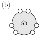
with complex coefficients g𝑔g called coupling constants. Different terms may have different coupling constants. Terms which can be obtained from each other by a cyclic permutation of matrices have identical trace and are thus equivalent from the point of view of the measure (44). It is therefore convenient to divide all terms into equivalence classes of products of X𝑋X and Xsuperscript𝑋X^{\dagger} which can be obtained from each other by a cyclic permutation. For example the following products X2X3X2superscript𝑋2superscript𝑋3superscript𝑋2X^{2}X^{3\dagger}X^{2}, X4X3superscript𝑋4superscript𝑋3X^{4}X^{3\dagger}, XX4X2superscript𝑋superscript𝑋4superscript𝑋2X^{\dagger}X^{4}X^{2\dagger} belong to the same equivalence class and have the same trace TrX2X3X2=TrX4X3=TrXX4X2Trsuperscript𝑋2superscript𝑋3superscript𝑋2Trsuperscript𝑋4superscript𝑋3Trsuperscript𝑋superscript𝑋4superscript𝑋2\mathrm{Tr}X^{2}X^{3\dagger}X^{2}=\mathrm{Tr}X^{4}X^{3\dagger}=\mathrm{Tr}X^{\dagger}X^{4}X^{2\dagger}. We call these equivalence classes periodic chains. We also define dual chains. A chain is said to be dual to a given chain if it is obtained by swapping positions of X𝑋X’s and Xsuperscript𝑋X^{\dagger}’s in the chain. The requirement that the trace of the potential is a real number means that the potential V(X,X)𝑉𝑋superscript𝑋V(X,X^{\dagger}) must contain pairs of dual terms with complex conjugate coupling constants. For example the terms gX2X𝑔superscript𝑋2superscript𝑋gX^{2}X^{\dagger} and g¯X2X¯𝑔superscript𝑋absent2𝑋\bar{g}X^{\dagger 2}X are mutually dual with proper coupling constants. For self-dual chains, as for instance gX2X2𝑔superscript𝑋2superscript𝑋2gX^{2}X^{2\dagger}, we have g=g¯𝑔¯𝑔g=\bar{g}, therefore those coupling constants must be real. For example the most general form of the third order terms in the potential is g1X3+g¯1X3+g2X2X+g¯2X2Xsubscript𝑔1superscript𝑋3subscript¯𝑔1superscript𝑋absent3subscript𝑔2superscript𝑋2superscript𝑋subscript¯𝑔2superscript𝑋absent2𝑋g_{1}X^{3}+\bar{g}_{1}X^{\dagger 3}+g_{2}X^{2}X^{\dagger}+\bar{g}_{2}X^{\dagger 2}X with two complex coupling constants denoted here by g1subscript𝑔1g_{1} and g2subscript𝑔2g_{2}. The fourth order potential has two dual pairs g3X4+g¯3X4subscript𝑔3superscript𝑋4subscript¯𝑔3superscript𝑋absent4g_{3}X^{4}+\bar{g}_{3}X^{\dagger 4} and g4X3X+g¯4X3Xsubscript𝑔4superscript𝑋3superscript𝑋subscript¯𝑔4superscript𝑋absent3𝑋g_{4}X^{3}X^{\dagger}+\bar{g}_{4}X^{\dagger 3}X, as well as two distinct self-dual terms g5X2X2subscript𝑔5superscript𝑋2superscript𝑋absent2g_{5}X^{2}X^{\dagger 2} and g6XXXXsubscript𝑔6𝑋superscript𝑋𝑋superscript𝑋g_{6}XX^{\dagger}XX^{\dagger} with real coupling constants g5subscript𝑔5g_{5} and g6subscript𝑔6g_{6}.

For convenience we assume, without loss of generality, that the measure is centered, that is 1NTrX=0delimited-⟨⟩1𝑁Tr𝑋0\langle\frac{1}{N}\mathrm{Tr}X\rangle=0, so we can skip linear terms in the potential. Next step is to split the measure into the gaussian part (43) and to treat the residual part as a perturbation of the gaussian measure bipz

dμ(X)=dμ0(X)eNTrVR(X,X)=dμ0(X)(1NTrVR(X,X)+12N2Tr2VR(X,X)+)𝑑𝜇𝑋𝑑subscript𝜇0𝑋superscript𝑒𝑁Trsubscript𝑉𝑅𝑋superscript𝑋𝑑subscript𝜇0𝑋1𝑁Trsubscript𝑉𝑅𝑋superscript𝑋12superscript𝑁2superscriptTr2subscript𝑉𝑅𝑋superscript𝑋d\mu(X)=d\mu_{0}(X)e^{-N\mathrm{Tr}V_{R}(X,X^{\dagger})}=d\mu_{0}(X)\left(1-N\mathrm{Tr}V_{R}(X,X^{\dagger})+\frac{1}{2}N^{2}\mathrm{Tr}^{2}V_{R}(X,X^{\dagger})+\ldots\right) (46)

where dμ0(X)𝑑subscript𝜇0𝑋d\mu_{0}(X) is the elliptic gaussian measure (43) and VRsubscript𝑉𝑅V_{R} is the remaining part of the potential which contains the third or higher order terms. In this way, the average of an observable O(X)𝑂𝑋O(X) is calculated as an average over the gaussian measure dμ0(X)𝑑subscript𝜇0𝑋d\mu_{0}(X) but of a new observable modified by terms coming from the perturbative expansion of the residual part

O(X)=O(X)(1NTrVR(X,X)+12N2Tr2VR(X,X)+)0.delimited-⟨⟩𝑂𝑋subscriptdelimited-⟨⟩𝑂𝑋1𝑁Trsubscript𝑉𝑅𝑋superscript𝑋12superscript𝑁2superscriptTr2subscript𝑉𝑅𝑋superscript𝑋0\langle O(X)\rangle=\left\langle O(X)\left(1-N\mathrm{Tr}V_{R}(X,X^{\dagger})+\frac{1}{2}N^{2}\mathrm{Tr}^{2}V_{R}(X,X^{\dagger})+\ldots\right)\right\rangle_{0}\ . (47)

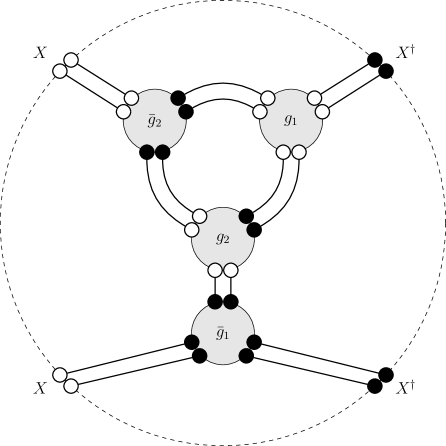
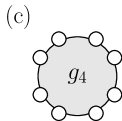
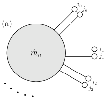
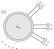
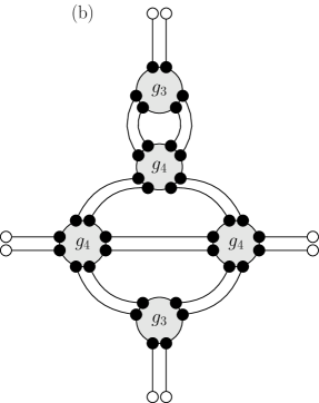
Now the calculation is reduced to gaussian integration. Thanks to the Wick’s theorem it can be mapped onto the problem of Feynman diagram enumeration which simplifies in the limit N𝑁N\rightarrow\infty to enumeration of planar diagrams th ; bipz . We will not give the details here, the interested reader can find them in bjn . We only give the Feynman rules for this model. Diagrams are constructed by drawing lines between vertices. The lines, called propagators, are deduced from the gaussian part dμ0(X)𝑑subscript𝜇0𝑋d\mu_{0}(X) (43). There are three different cases shown in Fig. 1 which correspond to two-point functions XX0subscriptdelimited-⟨⟩𝑋𝑋0\langle XX\rangle_{0}, XX0subscriptdelimited-⟨⟩𝑋superscript𝑋0\langle XX^{\dagger}\rangle_{0} XX0subscriptdelimited-⟨⟩superscript𝑋superscript𝑋0\langle X^{\dagger}X^{\dagger}\rangle_{0}. The vertices come from the expansion of the residual part. They correspond to different periodic chains. As an example, we show in Fig. 2 a diagram consisting two third order vertices contributing to XXXXdelimited-⟨⟩𝑋𝑋superscript𝑋superscript𝑋\left\langle XXX^{\dagger}X^{\dagger}\right\rangle. For each such diagram, there will be a dual one obtained by replacing matrices, XX𝑋superscript𝑋X\leftrightarrow X^{\dagger}, and vertices, gig¯isubscript𝑔𝑖subscript¯𝑔𝑖g_{i}\leftrightarrow\bar{g}_{i}, to their dual ones. The sum of all contributions from connected diagrams with n𝑛n external lines is equal to planar cumulant of order n𝑛n. Sometimes it is called a non-crossing cumulant or free cumulant of order n𝑛n. One can symbolically denote cumulants as connected averages 1NTrXaXbXcdelimited-⟨⟩delimited-⟨⟩1𝑁Trsuperscript𝑋𝑎superscript𝑋absent𝑏superscript𝑋𝑐\langle\langle\frac{1}{N}\mathrm{Tr}X^{a}X^{\dagger b}X^{c}\ldots\rangle\rangle. A cumulant of order n𝑛n is an array which contains connected averages for all distinct periodic chains of length n=a+b+c+𝑛𝑎𝑏𝑐n=a+b+c+\ldots. The R transform is a generating function of such cumulants (29). The main relation (15) between the Green function and R transform can be derived from the Dyson-Schwinger equations for planar diagrams. The details can be found in bjn .

Refer to caption

Refer to caption  , Refer to caption

Figure 1: Three possible propagators coming from gaussian part dμ0(X)𝑑subscript𝜇0𝑋d\mu_{0}\left(X\right) of the probability measure.
Refer to caption
Figure 2: Example of a diagram consisting of all four kinds of third order vertices (light gray circles), contributing to cumulant of order 4: TrX2X2delimited-⟨⟩delimited-⟨⟩Trsuperscript𝑋2superscript𝑋absent2\left\langle\left\langle\mathrm{Tr}X^{2}X^{\dagger 2}\right\rangle\right\rangle. The big dashed circle emphasises symmetry with respect to cyclic permutations under trace.

The R transform has an important property. The R transform of a sum A+B𝐴𝐵A+B of two independent random matrices, each defined by a probability measure of the type (44), is additive rj ; jnpz1

A+B(q)=A(q)+B(q).subscript𝐴𝐵𝑞subscript𝐴𝑞subscript𝐵𝑞\mathcal{R}_{A+B}(q)=\mathcal{R}_{A}(q)+\mathcal{R}_{B}(q)\ . (48)

This property can be easily understood in terms of Feynman diagrams. The measure dμ(A,B)=dμ(A)dμ(B)𝑑𝜇𝐴𝐵𝑑𝜇𝐴𝑑𝜇𝐵d\mu(A,B)=d\mu(A)d\mu(B) factorizes for independent matrices and also its gaussian part does dμ0(A,B)=dμ0(A)dμ0(B)𝑑subscript𝜇0𝐴𝐵𝑑subscript𝜇0𝐴𝑑subscript𝜇0𝐵d\mu_{0}(A,B)=d\mu_{0}(A)d\mu_{0}(B). As a consequence, the gaussian part does not contain mixed AB𝐴𝐵AB-terms and therefore the mixed propagators vanish AB0=AB0==0subscriptdelimited-⟨⟩𝐴𝐵0subscriptdelimited-⟨⟩𝐴superscript𝐵00\langle AB\rangle_{0}=\langle AB^{\dagger}\rangle_{0}=\ldots=0. This means that there are no lines in the Feynman diagrams which would directly connect vertices of type A𝐴A and B𝐵B. In effect, any connected diagram contains either vertices solely of type A𝐴A or vertices solely of type B𝐵B. In the former case they come from A(q)subscript𝐴𝑞\mathcal{R}_{A}(q) and in the latter one from B(q)subscript𝐵𝑞\mathcal{R}_{B}(q). Thus the generating function for connected diagrams A+B(q)subscript𝐴𝐵𝑞\mathcal{R}_{A+B}(q) splits into separate contributions from diagrams of type A𝐴A and of type B𝐵B: A(q)+B(q)subscript𝐴𝑞subscript𝐵𝑞\mathcal{R}_{A}(q)+\mathcal{R}_{B}(q). This is the standard diagrammatic interpretation of the additivity of cumulant generating functions.

One can work out consequences of the absence of mixed propagators also for the product AB𝐴𝐵AB of independent matrices. We do not show this calculation here and refer the interested reader to bjn . The multiplication law can be written in the form of three equations.

AB(𝒢AB)subscript𝐴𝐵subscript𝒢𝐴𝐵\displaystyle\mathcal{R}_{AB}\left(\mathcal{G}_{AB}\right) =[A(𝒢B)]L[B(𝒢A)]R,absentsuperscriptdelimited-[]subscript𝐴subscript𝒢𝐵𝐿superscriptdelimited-[]subscript𝐵subscript𝒢𝐴𝑅\displaystyle=\left[\mathcal{R}_{A}\left(\mathcal{G}_{B}\right)\right]^{L}\left[\mathcal{R}_{B}\left(\mathcal{G}_{A}\right)\right]^{R}, (49)
[𝒢A]Rsuperscriptdelimited-[]subscript𝒢𝐴𝑅\displaystyle\left[\mathcal{G}_{A}\right]^{R} =𝒢AB[A(𝒢B)]L,absentsubscript𝒢𝐴𝐵superscriptdelimited-[]subscript𝐴subscript𝒢𝐵𝐿\displaystyle=\mathcal{G}_{AB}\left[\mathcal{R}_{A}\left(\mathcal{G}_{B}\right)\right]^{L},
[𝒢B]Lsuperscriptdelimited-[]subscript𝒢𝐵𝐿\displaystyle\left[\mathcal{G}_{B}\right]^{L} =[B(𝒢A)]R𝒢AB,absentsuperscriptdelimited-[]subscript𝐵subscript𝒢𝐴𝑅subscript𝒢𝐴𝐵\displaystyle=\left[\mathcal{R}_{B}\left(\mathcal{G}_{A}\right)\right]^{R}\mathcal{G}_{AB},

Since now the R transforms are quaternionic (or matrix-valued) the order of multiplication matters. The quaternions 𝒢A=𝒢A(z^)subscript𝒢𝐴subscript𝒢𝐴^𝑧\mathcal{G}_{A}=\mathcal{G}_{A}(\hat{z}), 𝒢B=𝒢B(z^)subscript𝒢𝐵subscript𝒢𝐵^𝑧\mathcal{G}_{B}=\mathcal{G}_{B}(\hat{z}), 𝒢AB=𝒢AB(z^)subscript𝒢𝐴𝐵subscript𝒢𝐴𝐵^𝑧\mathcal{G}_{AB}=\mathcal{G}_{AB}(\hat{z}) in the last equation correspond to the Green’s functions for A𝐴A, B𝐵B and AB𝐴𝐵AB projected to the complex plane, that is calculated for quaternion z^=(z,0)^𝑧𝑧0\hat{z}=(z,0) having the second part equal zero. Quaternions tagged in the last equation by L𝐿L or R𝑅R correspond to left or right rotated copies of quaternions, given by the following transformations:

[𝒬]Lsuperscriptdelimited-[]𝒬𝐿\displaystyle\left[\mathcal{Q}\right]^{L} =U𝒬U,absent𝑈𝒬superscript𝑈\displaystyle=U\mathcal{Q}U^{\dagger},
[𝒬]Rsuperscriptdelimited-[]𝒬𝑅\displaystyle\left[\mathcal{Q}\right]^{R} =U𝒬U.absentsuperscript𝑈𝒬𝑈\displaystyle=U^{\dagger}\mathcal{Q}U. (50)

where U=diag(eiϕ/4,eiϕ/4)𝑈diagsuperscript𝑒𝑖italic-ϕ4superscript𝑒𝑖italic-ϕ4U=\mathrm{diag}\left(e^{i\phi/4},e^{-i\phi/4}\right) is a unitary matrix constructed from the phase of the complex number z=reiϕ𝑧𝑟superscript𝑒𝑖italic-ϕz=re^{i\phi}.

For hermitian matrices the quaternionic set of Eqs. (49) simplifies to a set of equations for R transforms RAsubscript𝑅𝐴R_{A}, RBsubscript𝑅𝐵R_{B} and RABsubscript𝑅𝐴𝐵R_{AB} being complex functions

RAB(z)subscript𝑅𝐴𝐵𝑧\displaystyle R_{AB}\left(z\right) =RA(w)RB(v),absentsubscript𝑅𝐴𝑤subscript𝑅𝐵𝑣\displaystyle=R_{A}\left(w\right)R_{B}\left(v\right), (51)
v𝑣\displaystyle v =zRA(w),absent𝑧subscript𝑅𝐴𝑤\displaystyle=zR_{A}\left(w\right),
w𝑤\displaystyle w =zRB(v).absent𝑧subscript𝑅𝐵𝑣\displaystyle=zR_{B}\left(v\right).

Moreover, if additionally the first cumulants of A𝐴A and B𝐵B are non-zero the last set of equations can be concisely written in this case in terms of the S transform v2

SAB(z)=SA(z)SB(z)subscript𝑆𝐴𝐵𝑧subscript𝑆𝐴𝑧subscript𝑆𝐵𝑧S_{AB}(z)=S_{A}(z)S_{B}(z) (52)

which is related to the R transform as follows bjn

SA(z)=1RA(zSA(z))orRA(z)=1SA(zRA(z)).formulae-sequencesubscript𝑆𝐴𝑧1subscript𝑅𝐴𝑧subscript𝑆𝐴𝑧orsubscript𝑅𝐴𝑧1subscript𝑆𝐴𝑧subscript𝑅𝐴𝑧S_{A}(z)=\frac{1}{R_{A}(zS_{A}(z))}\quad{\rm or}\quad R_{A}(z)=\frac{1}{S_{A}(zR_{A}(z))}\ . (53)

Unfortunately, there is no corresponding S transform representation of the multiplication law for non-hermitian matrices.

We finish this section by giving the transformation law for the R transform under multiplication of the matrix by a complex number: AA=αA𝐴superscript𝐴𝛼𝐴A\rightarrow A^{\prime}=\alpha A. Let us denote by α^^𝛼\hat{\alpha} a quaternion whose first Cayley-Dickson part is equal α𝛼\alpha and the second part is zero: α^=(α,0)^𝛼𝛼0\hat{\alpha}=(\alpha,0). One can see jn1 ; jn2 directly from the definition of the quaternionic Green’s function (6) that

𝒢αA(q)=𝒢A(α^1q)α^1.subscript𝒢𝛼𝐴𝑞subscript𝒢𝐴superscript^𝛼1𝑞superscript^𝛼1\mathcal{G}_{\alpha A}(q)=\mathcal{G}_{A}(\hat{\alpha}^{-1}q)\hat{\alpha}^{-1}\ . (54)

If follows from Eq. (15) that the R transform obeys the following transformation law under multiplication of the matrix by a complex number

αA(q)=α^A(qα^).subscript𝛼𝐴𝑞^𝛼subscript𝐴𝑞^𝛼{\mathcal{R}}_{\alpha A}(q)=\hat{\alpha}{\mathcal{R}}_{A}(q\hat{\alpha})\ . (55)

Additionally if we include constant shifts in the transformation law AA=x𝟙+αA𝐴superscript𝐴𝑥double-struck-𝟙𝛼𝐴A\rightarrow A^{\prime}=x\mathbb{1}+\alpha A we obtain

A(q)=x^+α^A(qα^).subscriptsuperscript𝐴𝑞^𝑥^𝛼subscript𝐴𝑞^𝛼{\mathcal{R}}_{A^{\prime}}(q)=\hat{x}+\hat{\alpha}{\mathcal{R}}_{A}(q\hat{\alpha})\ . (56)

In particular when we apply this transformation to the standardized elliptic gaussian law (36) we obtain the general form (37).

As an example of the application of this transformation law let us derive the R transform for X=12(A+iB)𝑋12𝐴𝑖𝐵X=\frac{1}{\sqrt{2}}\left(A+iB\right) where A𝐴A and B𝐵B are standardized independent gaussian hermitian matrices: A(q)=B(q)=qsubscript𝐴𝑞subscript𝐵𝑞𝑞\mathcal{R}_{A}(q)=\mathcal{R}_{B}(q)=q. Using the addition law (48) and the transformation (55) for rescaling we easily find in agreement with jn1 ; jn2

X((z,w))=12(z,w)+12(i,0)(z,w)(i,0)=(0,w),subscript𝑋𝑧𝑤12𝑧𝑤12𝑖0𝑧𝑤𝑖00𝑤\mathcal{R}_{X}((z,w))=\frac{1}{2}(z,w)+\frac{1}{2}(i,0)(z,w)(i,0)=(0,w)\ , (57)

where the argument of the R transform is written as a Cayley-Dickson pair q=(z,w)𝑞𝑧𝑤q=(z,w). In the last step of the calculation we applied Eq. (103). As expected, we reconstructed the R transform for the Ginibre matrices. For pedagogical reasons we rewrite the last equation in the matrix representation (105) which is better known

X((zww¯z¯))=12(zww¯z¯)+12(i00i)(zww¯z¯)(i00i)=(0ww¯0).subscript𝑋𝑧𝑤¯𝑤¯𝑧12𝑧𝑤¯𝑤¯𝑧12𝑖00𝑖𝑧𝑤¯𝑤¯𝑧𝑖00𝑖0𝑤¯𝑤0\mathcal{R}_{X}\left(\left(\begin{array}[]{cc}z&w\\ -\bar{w}&\bar{z}\end{array}\right)\right)=\frac{1}{2}\left(\begin{array}[]{cc}z&w\\ -\bar{w}&\bar{z}\end{array}\right)+\frac{1}{2}\left(\begin{array}[]{cc}i&0\\ 0&-i\end{array}\right)\left(\begin{array}[]{cc}z&w\\ -\bar{w}&\bar{z}\end{array}\right)\left(\begin{array}[]{cc}i&0\\ 0&-i\end{array}\right)=\left(\begin{array}[]{cc}0&w\\ -\bar{w}&0\end{array}\right). (58)

VI Applications of quaternionic R transform

In this section, as an illustration, we give several examples of how to calculate eigenvalue densities of sums and products of gaussian elliptic random matrices using the quaternionic R transform.

VI.1 Sums of gaussian random matrices

It is easy to see that a sum C=A+B𝐶𝐴𝐵C=A+B of gaussian elliptic matrices A𝐴A and B𝐵B is again an elliptic gaussian random matrix. Denote the R transforms (37) for A𝐴A and B𝐵B as A(z+wj)=xA+σA2(μAe2iϕAz+wj)subscript𝐴𝑧𝑤𝑗subscript𝑥𝐴subscriptsuperscript𝜎2𝐴subscript𝜇𝐴superscript𝑒2𝑖subscriptitalic-ϕ𝐴𝑧𝑤𝑗\mathcal{R}_{A}(z+wj)=x_{A}+\sigma^{2}_{A}\left(\mu_{A}e^{2i\phi_{A}}z+wj\right) and B(z+wj)=xB+σB2(μBe2iϕBz+wj)subscript𝐵𝑧𝑤𝑗subscript𝑥𝐵subscriptsuperscript𝜎2𝐵subscript𝜇𝐵superscript𝑒2𝑖subscriptitalic-ϕ𝐵𝑧𝑤𝑗\mathcal{R}_{B}(z+wj)=x_{B}+\sigma^{2}_{B}\left(\mu_{B}e^{2i\phi_{B}}z+wj\right). As follows from the addition law (48) the R transform for C𝐶C has exactly the same form C(z+wj)=xC+σC2(μCe2iϕCz+wj)subscript𝐶𝑧𝑤𝑗subscript𝑥𝐶subscriptsuperscript𝜎2𝐶subscript𝜇𝐶superscript𝑒2𝑖subscriptitalic-ϕ𝐶𝑧𝑤𝑗\mathcal{R}_{C}(z+wj)=x_{C}+\sigma^{2}_{C}\left(\mu_{C}e^{2i\phi_{C}}z+wj\right) with xC=xA+xBsubscript𝑥𝐶subscript𝑥𝐴subscript𝑥𝐵x_{C}=x_{A}+x_{B}, σC2=σA2+σB2subscriptsuperscript𝜎2𝐶subscriptsuperscript𝜎2𝐴subscriptsuperscript𝜎2𝐵\sigma^{2}_{C}=\sigma^{2}_{A}+\sigma^{2}_{B}, μCeiϕC=(μAσA2eiϕA+μBσB2eiϕB)/(σA2+σB2)subscript𝜇𝐶superscript𝑒𝑖subscriptitalic-ϕ𝐶subscript𝜇𝐴subscriptsuperscript𝜎2𝐴superscript𝑒𝑖subscriptitalic-ϕ𝐴subscript𝜇𝐵subscriptsuperscript𝜎2𝐵superscript𝑒𝑖subscriptitalic-ϕ𝐵superscriptsubscript𝜎𝐴2superscriptsubscript𝜎𝐵2\mu_{C}e^{i\phi_{C}}=(\mu_{A}\sigma^{2}_{A}e^{i\phi_{A}}+\mu_{B}\sigma^{2}_{B}e^{i\phi_{B}})/(\sigma_{A}^{2}+\sigma_{B}^{2}). In other words, the elliptic gaussian laws are stable under addition. In particular if we add a Ginibre matrix X𝑋X (xA=0,μA=0,σA=1,ϕA=0formulae-sequencesubscript𝑥𝐴0formulae-sequencesubscript𝜇𝐴0formulae-sequencesubscript𝜎𝐴1subscriptitalic-ϕ𝐴0x_{A}=0,\mu_{A}=0,\sigma_{A}=1,\phi_{A}=0) to a hermitian GUE matrix H𝐻H m (xA=0,μB=1,σB=1,ϕB=0formulae-sequencesubscript𝑥𝐴0formulae-sequencesubscript𝜇𝐵1formulae-sequencesubscript𝜎𝐵1subscriptitalic-ϕ𝐵0x_{A}=0,\mu_{B}=1,\sigma_{B}=1,\phi_{B}=0) we obtain a matrix C=X+H𝐶𝑋𝐻C=X+H with the R transform C(z+wj)=z+2wjsubscript𝐶𝑧𝑤𝑗𝑧2𝑤𝑗\mathcal{R}_{C}(z+wj)=z+2wj. The corresponding eigenvalue density is uniform on an ellipse located at the origin of the complex plane with the longer semi-axis of length 22\sqrt{2} on the real axis and the shorter one of length 111 on the imaginary axis. This is schematically shown in Fig. 3.

Refer to caption

,

Figure 3: Schematic representation of addition law in case of sum of Ginibre and GUE matrices, which results in Elliptic matrix.

VI.2 Products of gaussian random matrices

The eigenvalue density of a product of gaussian elliptic random matrices can be calculated from the general multiplication law Eqs. (49) and the Eq. (28)

𝒢AB(z^)=1z^AB(𝒢AB(z^))subscript𝒢𝐴𝐵^𝑧1^𝑧subscript𝐴𝐵subscript𝒢𝐴𝐵^𝑧\mathcal{G}_{AB}\left(\hat{z}\right)=\frac{1}{\hat{z}-\mathcal{R}_{AB}\left(\mathcal{G}_{AB}\left(\hat{z}\right)\right)}\ (59)

which relates the Green’s function and the R transform for the product AB𝐴𝐵AB. From these equations we obtain the Green’s function 𝒢AB(z^)subscript𝒢𝐴𝐵^𝑧\mathcal{G}_{AB}\left(\hat{z}\right) on the complex plane that is for quaternions having the second part equal zero z^=(z,0)^𝑧𝑧0\hat{z}=(z,0). Then we extract the first part of the quaternionic Green’s function

GAB(z)=F𝒢AB(z^)subscript𝐺𝐴𝐵𝑧𝐹subscript𝒢𝐴𝐵^𝑧G_{AB}(z)=F\mathcal{G}_{AB}\left(\hat{z}\right) (60)

which is a complex function GAB(z)subscript𝐺𝐴𝐵𝑧G_{AB}(z) and eventually we use Eq. (12) to calculate the eigenvalue density

ρAB(z)=1πGAB(z)z¯.subscript𝜌𝐴𝐵𝑧1𝜋subscript𝐺𝐴𝐵𝑧¯𝑧\rho_{AB}(z)=\frac{1}{\pi}\frac{\partial G_{AB}(z)}{\partial\bar{z}}. (61)

Let us give a couple of examples. For convenience we introduce a shorthand notation. We denote the standardized elliptic matrix with the eccentricity parameter μ𝜇\mu by E(μ)𝐸𝜇E(\mu) gi . The matrix E(μ)𝐸𝜇E(\mu) has the following quaternionic R transform E(μ)(z+wj)=μ+wjsubscript𝐸𝜇𝑧𝑤𝑗𝜇𝑤𝑗\mathcal{R}_{E(\mu)}(z+wj)=\mu+wj, or in the matrix representation

E(μ)((zww¯z¯))=(μzww¯μz¯).subscript𝐸𝜇𝑧𝑤¯𝑤¯𝑧𝜇𝑧𝑤¯𝑤𝜇¯𝑧\mathcal{R}_{E(\mu)}\left(\left(\begin{array}[]{rr}z&w\\ -\bar{w}&\bar{z}\end{array}\right)\right)=\left(\begin{array}[]{rr}\mu z&w\\ -\bar{w}&\mu\bar{z}\end{array}\right). (62)

We reserve a special notation for the standardized Ginibre matrices X=E(0)𝑋𝐸0X=E(0) and the standardized hermitian GUE matrix by H=E(1)𝐻𝐸1H=E(1). Let us note that the Ginibre ensemble is invariant under rotation XX=eiϕX𝑋superscript𝑋superscript𝑒𝑖italic-ϕ𝑋X\rightarrow X^{\prime}=e^{i\phi}X. Indeed, using the transformation law (55) we see that

X((zww¯z¯))=(eiϕ00eiϕ)(0ww¯0)(eiϕ00eiϕ)=(0ww¯0)=X((zww¯z))subscriptsuperscript𝑋𝑧𝑤¯𝑤¯𝑧superscript𝑒𝑖italic-ϕ00superscript𝑒𝑖italic-ϕ0𝑤¯𝑤0superscript𝑒𝑖italic-ϕ00superscript𝑒𝑖italic-ϕ0𝑤¯𝑤0subscript𝑋𝑧𝑤¯𝑤𝑧\mathcal{R}_{X^{\prime}}\left(\left(\begin{array}[]{rr}z&w\\ -\bar{w}&\bar{z}\end{array}\right)\right)=\left(\begin{array}[]{cc}e^{i\phi}&0\\ 0&e^{-i\phi}\end{array}\right)\left(\begin{array}[]{rr}0&w\\ -\bar{w}&0\end{array}\right)\left(\begin{array}[]{cc}e^{i\phi}&0\\ 0&e^{-i\phi}\end{array}\right)=\left(\begin{array}[]{rr}0&w\\ -\bar{w}&0\end{array}\right)=\mathcal{R}_{X}\left(\left(\begin{array}[]{rr}z&w\\ -\bar{w}&z\end{array}\right)\right) (63)

the R transform stays intact unter the multiplication of the Ginibre matrix by the phase factor eiϕsuperscript𝑒𝑖italic-ϕe^{i\phi}. Now we are ready to consider examples.

We use the Pauli matrix representation for practical calculations, because complex algebra is familiar to all readers and is well implemented in many software packages, which is not the case for quaternions.

The first example is the product of A=a𝟙+bX1𝐴𝑎double-struck-𝟙𝑏subscript𝑋1A=a\mathbb{1}+bX_{1} and B=c𝟙+dX2𝐵𝑐double-struck-𝟙𝑑subscript𝑋2B=c\mathbb{1}+dX_{2}

AB=(a𝟙+bX1)(c𝟙+dX2),𝐴𝐵𝑎double-struck-𝟙𝑏subscript𝑋1𝑐double-struck-𝟙𝑑subscript𝑋2AB=\left(a\mathbb{1}+bX_{1}\right)\left(c\mathbb{1}+dX_{2}\right), (64)

where a,b,c,d𝑎𝑏𝑐𝑑a,b,c,d\in\mathbb{C}, b,d0𝑏𝑑0b,d\neq 0 and X1,X2subscript𝑋1subscript𝑋2X_{1},X_{2} are independent standardized Ginibre matrices. The question we ask here is: what is the eigenvalue spectrum of the product? For such a product one can easily see, using the invariance of the Ginibre ensemble under the multiplication XX=eiϕX𝑋superscript𝑋superscript𝑒𝑖italic-ϕ𝑋X\rightarrow X^{\prime}=e^{i\phi}X (63), that the following redefinition of parameters:

s=|ab|,t=|cd|,u=|bd|eiArg(ac),formulae-sequence𝑠𝑎𝑏formulae-sequence𝑡𝑐𝑑𝑢𝑏𝑑superscript𝑒𝑖Arg𝑎𝑐s=\left|\frac{a}{b}\right|,\quad t=\left|\frac{c}{d}\right|,\quad u=|bd|e^{i\mathrm{Arg}(ac)}, (65)

reduces the calculations to the problem of finding the eigenvalue density of a matrix

u(s𝟙+X1)(t𝟙+X2),𝑢𝑠double-struck-𝟙subscript𝑋1𝑡double-struck-𝟙subscript𝑋2u\left(s\mathbb{1}+X_{1}\right)\left(t\mathbb{1}+X_{2}\right), (66)

where s,t+𝑠𝑡subscripts,t\in\mathbb{R}_{+}. The parameter u𝑢u scales the eigenvalue density with |u|𝑢\left|u\right| and rotates it around the center of the complex plane by Arg(u)Arg𝑢\mathrm{Arg}\left(u\right) angle. This means that it is sufficient to consider products of the type

AB=(s𝟙+X1)(t𝟙+X2)𝐴𝐵𝑠double-struck-𝟙subscript𝑋1𝑡double-struck-𝟙subscript𝑋2AB=\left(s\mathbb{1}+X_{1}\right)\left(t\mathbb{1}+X_{2}\right) (67)

without loss of generality. Using the addition law (48) for matrices A=s𝟙+X𝐴𝑠double-struck-𝟙𝑋A=s\mathbb{1}+X and B=t𝟙+X𝐵𝑡double-struck-𝟙𝑋B=t\mathbb{1}+X we have

A((wBvBv¯Bw¯B))=(svBv¯Bs¯),subscript𝐴subscript𝑤𝐵subscript𝑣𝐵subscript¯𝑣𝐵subscript¯𝑤𝐵𝑠subscript𝑣𝐵subscript¯𝑣𝐵¯𝑠\mathcal{R}_{A}\left(\left(\begin{array}[]{cc}w_{B}&v_{B}\\ -\bar{v}_{B}&\bar{w}_{B}\\ \end{array}\right)\right)=\left(\begin{array}[]{cc}s&v_{B}\\ -\bar{v}_{B}&\bar{s}\\ \end{array}\right), (68)

and

B((wAvAv¯Aw¯A))=(tvAv¯At¯),subscript𝐵subscript𝑤𝐴subscript𝑣𝐴subscript¯𝑣𝐴subscript¯𝑤𝐴𝑡subscript𝑣𝐴subscript¯𝑣𝐴¯𝑡\mathcal{R}_{B}\left(\left(\begin{array}[]{cc}w_{A}&v_{A}\\ -\bar{v}_{A}&\bar{w}_{A}\\ \end{array}\right)\right)=\left(\begin{array}[]{cc}t&v_{A}\\ -\bar{v}_{A}&\bar{t}\\ \end{array}\right), (69)

respectively. Since s𝑠s and t𝑡t are real we may omit their complex conjugation. Inserting Eqs. (68,69) to the multiplication law formulas (49) and writing z𝑧z in the polar form z=reiϕ𝑧𝑟superscript𝑒𝑖italic-ϕz=re^{i\phi} we get the R transform for the product:

AB(𝒢AB)=(stv¯AvBeiϕtvAeiϕ/2+svBeiϕ/2tv¯Aeiϕ/2sv¯Beiϕ/2stvAv¯Beiϕ).subscript𝐴𝐵subscript𝒢𝐴𝐵𝑠𝑡subscript¯𝑣𝐴subscript𝑣𝐵superscript𝑒𝑖italic-ϕ𝑡subscript𝑣𝐴superscript𝑒𝑖italic-ϕ2𝑠subscript𝑣𝐵superscript𝑒𝑖italic-ϕ2𝑡subscript¯𝑣𝐴superscript𝑒𝑖italic-ϕ2𝑠subscript¯𝑣𝐵superscript𝑒𝑖italic-ϕ2𝑠𝑡subscript𝑣𝐴subscript¯𝑣𝐵superscript𝑒𝑖italic-ϕ\displaystyle\mathcal{R}_{AB}\left(\mathcal{G}_{AB}\right)=\left(\begin{array}[]{cc}st-\bar{v}_{A}v_{B}e^{i\phi}&tv_{A}e^{-i\phi/2}+sv_{B}e^{i\phi/2}\\ -t\bar{v}_{A}e^{i\phi/2}-s\bar{v}_{B}e^{-i\phi/2}&st-v_{A}\bar{v}_{B}e^{-i\phi}\end{array}\right). (72)

Now using Eq. (59) we obtain the quaternionic Green’s function on the complex plane. Its first Cayley-Dickson part reads

GAB(z)=streiϕvAv¯Bs2t2+r2+t2|vA|2+s2|vB|2+r(vAv¯B+v¯AvB)+|vA|2|vB|22strcosϕ.subscript𝐺𝐴𝐵𝑧𝑠𝑡𝑟superscript𝑒𝑖italic-ϕsubscript𝑣𝐴subscript¯𝑣𝐵superscript𝑠2superscript𝑡2superscript𝑟2superscript𝑡2superscriptsubscript𝑣𝐴2superscript𝑠2superscriptsubscript𝑣𝐵2𝑟subscript𝑣𝐴subscript¯𝑣𝐵subscript¯𝑣𝐴subscript𝑣𝐵superscriptsubscript𝑣𝐴2superscriptsubscript𝑣𝐵22𝑠𝑡𝑟italic-ϕG_{AB}(z)=-\frac{st-re^{-i\phi}-v_{A}\bar{v}_{B}}{s^{2}t^{2}+r^{2}+t^{2}\left|v_{A}\right|^{2}+s^{2}\left|v_{B}\right|^{2}+r(v_{A}\bar{v}_{B}+\bar{v}_{A}v_{B})+\left|v_{A}\right|^{2}\left|v_{B}\right|^{2}-2str\cos\phi}. (73)

Now we have to find vAsubscript𝑣𝐴v_{A} and vBsubscript𝑣𝐵v_{B} as a function of complex argument z𝑧z (or equivalently r𝑟r and ϕitalic-ϕ\phi). To this end we utilize the second and third quaternionic equations in (49) that are equivalent to the following four independent complex equations

t|vA|2+eiϕ(wAr+v¯AvB(s+wA))𝑡superscriptsubscript𝑣𝐴2superscript𝑒𝑖italic-ϕsubscript𝑤𝐴𝑟subscript¯𝑣𝐴subscript𝑣𝐵𝑠subscript𝑤𝐴\displaystyle t\left|v_{A}\right|^{2}+e^{i\phi}\left(w_{A}r+\bar{v}_{A}v_{B}\left(s+w_{A}\right)\right) =t(1+swA),absent𝑡1𝑠subscript𝑤𝐴\displaystyle=t(1+sw_{A}), (74)
s|vB|2+eiϕ(wBr+vAv¯B(t+wB))𝑠superscriptsubscript𝑣𝐵2superscript𝑒𝑖italic-ϕsubscript𝑤𝐵𝑟subscript𝑣𝐴subscript¯𝑣𝐵𝑡subscript𝑤𝐵\displaystyle s\left|v_{B}\right|^{2}+e^{i\phi}\left(w_{B}r+v_{A}\bar{v}_{B}\left(t+w_{B}\right)\right) =s(1+twB),absent𝑠1𝑡subscript𝑤𝐵\displaystyle=s(1+tw_{B}), (75)
eiϕ(sw¯AvB+vB|vA|2+vArvB)superscript𝑒𝑖italic-ϕ𝑠subscript¯𝑤𝐴subscript𝑣𝐵subscript𝑣𝐵superscriptsubscript𝑣𝐴2subscript𝑣𝐴𝑟subscript𝑣𝐵\displaystyle e^{i\phi}\left(-s\bar{w}_{A}v_{B}+v_{B}\left|v_{A}\right|^{2}+v_{A}r-v_{B}\right) =tvA(s+w¯A),absent𝑡subscript𝑣𝐴𝑠subscript¯𝑤𝐴\displaystyle=tv_{A}\left(s+\bar{w}_{A}\right), (76)
eiϕ(twBvA+vA|vB|2+vBrvA)superscript𝑒𝑖italic-ϕ𝑡subscript𝑤𝐵subscript𝑣𝐴subscript𝑣𝐴superscriptsubscript𝑣𝐵2subscript𝑣𝐵𝑟subscript𝑣𝐴\displaystyle e^{-i\phi}\left(-tw_{B}v_{A}+v_{A}\left|v_{B}\right|^{2}+v_{B}r-v_{A}\right) =svB(t+wB).absent𝑠subscript𝑣𝐵𝑡subscript𝑤𝐵\displaystyle=sv_{B}\left(t+w_{B}\right). (77)

The last two equations have a trivial solution: vA=vB=0subscript𝑣𝐴subscript𝑣𝐵0v_{A}=v_{B}=0. It corresponds to the holomorphic part of Green’s function, G(z)=(zst)1𝐺𝑧superscript𝑧𝑠𝑡1G\left(z\right)=(z-st)^{-1}, valid outside the eigenvalue domain.

By some algebraic manipulations in Eq. (76) we may express vBsubscript𝑣𝐵v_{B} as

vB=vAαβ|vA|2,subscript𝑣𝐵subscript𝑣𝐴𝛼𝛽superscriptsubscript𝑣𝐴2v_{B}=v_{A}\frac{\alpha}{\beta-\left|v_{A}\right|^{2}}, (78)

which means that combinations vAv¯Bsubscript𝑣𝐴subscript¯𝑣𝐵v_{A}\bar{v}_{B} and v¯AvBsubscript¯𝑣𝐴subscript𝑣𝐵\bar{v}_{A}v_{B} do not depend on phases of vAsubscript𝑣𝐴v_{A} and vBsubscript𝑣𝐵v_{B}. Indeed an inspection of the expression for the Green’s function (73) shows, that it depends on vAsubscript𝑣𝐴v_{A} and vBsubscript𝑣𝐵v_{B} only through the moduli |vA|subscript𝑣𝐴\left|v_{A}\right|,|vB|subscript𝑣𝐵\left|v_{B}\right|. Their phases are also irrelevant in Eqs. (76,77). In fact, this is true for any product of elliptic ensembles. For the rest of the discussion those phases will be set to 00, so vA=v¯Asubscript𝑣𝐴subscript¯𝑣𝐴v_{A}=\bar{v}_{A}, vB=v¯Bsubscript𝑣𝐵subscript¯𝑣𝐵v_{B}=\bar{v}_{B} and vA,vB+subscript𝑣𝐴subscript𝑣𝐵subscriptv_{A},v_{B}\in\mathbb{R_{+}}. Solving Eqs. (74,75,76,77) for vAsubscript𝑣𝐴v_{A} and vBsubscript𝑣𝐵v_{B} yields:

vA(1+vA2+s2)(vB2+t2)+(1+2vA2)vBr+vAr22stvArcosϕ=0,subscript𝑣𝐴1superscriptsubscript𝑣𝐴2superscript𝑠2superscriptsubscript𝑣𝐵2superscript𝑡212superscriptsubscript𝑣𝐴2subscript𝑣𝐵𝑟subscript𝑣𝐴superscript𝑟22𝑠𝑡subscript𝑣𝐴𝑟italic-ϕ0\displaystyle v_{A}(-1+v_{A}^{2}+s^{2})(v_{B}^{2}+t^{2})+(-1+2v_{A}^{2})v_{B}r+v_{A}r^{2}-2stv_{A}r\cos\phi=0, (79)
vB(1+vB2+t2)(vA2+s2)+(1+2vB2)vAr+vBr22stvBrcosϕ=0.subscript𝑣𝐵1superscriptsubscript𝑣𝐵2superscript𝑡2superscriptsubscript𝑣𝐴2superscript𝑠212superscriptsubscript𝑣𝐵2subscript𝑣𝐴𝑟subscript𝑣𝐵superscript𝑟22𝑠𝑡subscript𝑣𝐵𝑟italic-ϕ0\displaystyle v_{B}(-1+v_{B}^{2}+t^{2})(v_{A}^{2}+s^{2})+(-1+2v_{B}^{2})v_{A}r+v_{B}r^{2}-2stv_{B}r\cos\phi=0. (80)

Note that those equations are invariant under the simultaneous change of sings vAvAsubscript𝑣𝐴subscript𝑣𝐴v_{A}\rightarrow-v_{A} and vBvBsubscript𝑣𝐵subscript𝑣𝐵v_{B}\rightarrow-v_{B} which is a remnant of the symmetry of v𝑣v’s mentioned above. In effect if vAsubscript𝑣𝐴v_{A} and vBsubscript𝑣𝐵v_{B} is a solution to these equations, then also vA=vAsuperscriptsubscript𝑣𝐴subscript𝑣𝐴v_{A}^{\prime}=-v_{A} and vB=vBsuperscriptsubscript𝑣𝐵subscript𝑣𝐵v_{B}^{\prime}=-v_{B} is a solution that gives the same Green’s function, leading to the same eigenvalue density.

The eigenvalue density is represented as a function with a compact support on the complex plane. Let us focus on the outline (contour) of this support. We may calculate it by matching the holomorphic (vA=vB=0subscript𝑣𝐴subscript𝑣𝐵0v_{A}=v_{B}=0) and non-holomorphic solutions. To do so, we solve quadratic Eq. (79) for vBsubscript𝑣𝐵v_{B}, and pick the leading term of the solution, that vanishes in the limit vA0subscript𝑣𝐴0v_{A}\rightarrow 0. Then by inserting this solution into Eq.(79), and performing the limit vA0subscript𝑣𝐴0v_{A}\rightarrow 0 we are left with the following equation

(s2t2s4t2s2t4+s4t4)+(2s3tcosϕ+2st3cosϕ4s3t3cosϕ)r+superscript𝑠2superscript𝑡2superscript𝑠4superscript𝑡2superscript𝑠2superscript𝑡4superscript𝑠4superscript𝑡4limit-from2superscript𝑠3𝑡italic-ϕ2𝑠superscript𝑡3italic-ϕ4superscript𝑠3superscript𝑡3italic-ϕ𝑟\displaystyle(s^{2}t^{2}-s^{4}t^{2}-s^{2}t^{4}+s^{4}t^{4})+(2s^{3}t\cos\phi+2st^{3}\cos\phi-4s^{3}t^{3}\cos\phi)r+ (81)
+\displaystyle+ (1s2t2+2s2t2+4s2t2cos2ϕ)r24stcosϕr3+r4=0,1superscript𝑠2superscript𝑡22superscript𝑠2superscript𝑡24superscript𝑠2superscript𝑡2superscript2italic-ϕsuperscript𝑟24𝑠𝑡italic-ϕsuperscript𝑟3superscript𝑟40\displaystyle(-1-s^{2}-t^{2}+2s^{2}t^{2}+4s^{2}t^{2}\cos^{2}\phi)r^{2}-4st\cos\phi\ r^{3}+r^{4}=0,

which may be treated as a fourth order polynomial equation for r𝑟r and solved for any value of ϕitalic-ϕ\phi giving the contour of the eigenvalue distribution.

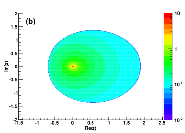
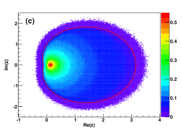
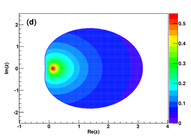
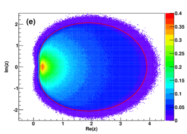
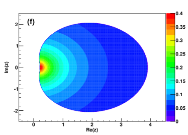
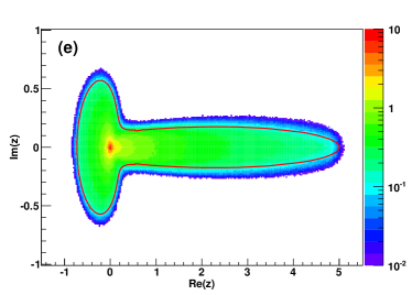
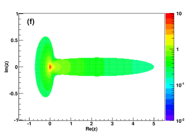
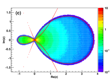
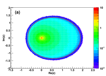
Now the remaining part is to numerically solve real polynomial Eqs. (79,80), e.g. on a lattice inside the previously calculated domain, plug the results into Eq. (73) and calculate eigenvalue density according to Eq. (12). The results for several different values of s𝑠s and t𝑡t are shown in Fig. 4, together with comparison to numerical simulations. The agreement is very good. Due to the finite size effects the edges of the support are smeared and instead of a sharp edge on the contour line there is a crossover region of width that decreases with N𝑁N where the eigenvalue density falls off to zero.

The equation (LABEL:eq:s+X_t+X_contour) is general in the sense that it holds for any t𝑡t and s𝑠s. The special symmetric case t=s𝑡𝑠t=s can be solved in a simpler way. The symmetry AB𝐴𝐵A\longleftrightarrow B which holds in this case significantly reduces the complexity of the problem because one may at the beginning of the calculation set wA=wBsubscript𝑤𝐴subscript𝑤𝐵w_{A}=w_{B} and vA=vBsubscript𝑣𝐴subscript𝑣𝐵v_{A}=v_{B} and reduce the number of unknown variables. Two special cases: t=s=0𝑡𝑠0t=s=0 and t=s=1𝑡𝑠1t=s=1 of this symmetric problem have been discussed previously bjn and can be used as a cross-check of our general formula (LABEL:eq:s+X_t+X_contour). The case t=s=0𝑡𝑠0t=s=0 corresponds to the product of two standardized Ginibre matrices with the contour given by the equation bjw

r21=0.superscript𝑟210r^{2}-1=0\ . (82)

The case t=s=1𝑡𝑠1t=s=1 corresponds to the product of two standardized Ginibre matrices shfited by unit matrix and has the contour given by the equation

r24cosϕr+4cos2ϕ1=(r2cosϕ1)(r2cosϕ+1)=0.superscript𝑟24italic-ϕ𝑟4superscript2italic-ϕ1𝑟2italic-ϕ1𝑟2italic-ϕ10r^{2}-4\cos\phi\ r+4\cos^{2}\phi\ -1=(r-2\cos\phi\ -1)(r-2\cos\phi\ +1)=0. (83)

The first one gives a circle and the second one a Pascal limaçon, in agreement with gjjn ; bjn .
Refer to caption
Refer to caption
Refer to caption
Refer to caption
Refer to caption
Refer to caption
Figure 4: (Color online) Numerical eigenvalue distributions for matrices (s𝟙+X)(t𝟙+X)𝑠double-struck-𝟙𝑋𝑡double-struck-𝟙𝑋(s\mathbb{1}+X)(t\mathbb{1}+X) 100×100100100100\times 100 for (a) s=0.50𝑠0.50s=0.50,t=0.75𝑡0.75t=0.75 (c) s=0.9𝑠0.9s=0.9,t=1.2𝑡1.2t=1.2 and (e) s=1.2𝑠1.2s=1.2,t=1.3𝑡1.3t=1.3 compared with theoretically evaluated ones in (b),(d) and (f) respectively. The edge of the distribution is shown on the plots (a),(c) and (e) (red curve). Each histogram is made from 107superscript10710^{7} eigenvalues.

The second example we consider is a product

AB=(𝟙+E1(μ))(𝟙+E2(μ)),𝐴𝐵double-struck-𝟙subscript𝐸1𝜇double-struck-𝟙subscript𝐸2𝜇AB=(\mathbb{1}+E_{1}(\mu))(\mathbb{1}+E_{2}(\mu)), (84)

of two independent identically distributed shifted elliptic matrices A=𝟙+E1(μ)𝐴double-struck-𝟙subscript𝐸1𝜇A=\mathbb{1}+E_{1}(\mu) and B=𝟙+E2(μ)𝐵double-struck-𝟙subscript𝐸2𝜇B=\mathbb{1}+E_{2}(\mu). We follow exactly the same procedure as in the first example except that now we exploit the invariance of the problem under the exchange E1(μ)E2(μ)subscript𝐸1𝜇subscript𝐸2𝜇E_{1}(\mu)\longleftrightarrow E_{2}(\mu) to make a symmetric Ansatz wA=wB=wsubscript𝑤𝐴subscript𝑤𝐵𝑤w_{A}=w_{B}=w and vA=vB=vsubscript𝑣𝐴subscript𝑣𝐵𝑣v_{A}=v_{B}=v at the beginning of the calculations. This simplifies the problem remarkably. The R transform for a shifted elliptic matrix is given by (37)

((wvv¯w¯))=(1+wμvv¯1+w¯μ),𝑤𝑣¯𝑣¯𝑤1𝑤𝜇𝑣¯𝑣1¯𝑤𝜇\mathcal{R}\left(\left(\begin{array}[]{cc}w&v\\ -\bar{v}&\bar{w}\end{array}\right)\right)=\left(\begin{array}[]{cc}1+w\mu&v\\ -\bar{v}&1+\bar{w}\mu\end{array}\right), (85)

and for the product:

AB(𝒢AB)=((1+wμ)2|v|2eiϕv(eiϕ/2(1+wμ)+eiϕ/2(1+w¯μ))v¯(eiϕ/2(1+wμ)+eiϕ/2(1+w¯μ))(1+w¯μ)2|v|2eiϕ).subscript𝐴𝐵subscript𝒢𝐴𝐵superscript1𝑤𝜇2superscript𝑣2superscript𝑒𝑖italic-ϕ𝑣superscript𝑒𝑖italic-ϕ21𝑤𝜇superscript𝑒𝑖italic-ϕ21¯𝑤𝜇¯𝑣superscript𝑒𝑖italic-ϕ21𝑤𝜇superscript𝑒𝑖italic-ϕ21¯𝑤𝜇superscript1¯𝑤𝜇2superscript𝑣2superscript𝑒𝑖italic-ϕ\mathcal{R}_{AB}\left(\mathcal{G}_{AB}\right)=\left(\begin{array}[]{cc}\left(1+w\mu\right)^{2}-\left|v\right|^{2}e^{i\phi}&v\left(e^{-i\phi/2}\left(1+w\mu\right)+e^{i\phi/2}\left(1+\bar{w}\mu\right)\right)\\ -\bar{v}\left(e^{-i\phi/2}(1+w\mu)+e^{i\phi/2}(1+\bar{w}\mu)\right)&\left(1+\bar{w}\mu\right)^{2}-\left|v\right|^{2}e^{-i\phi}\end{array}\right). (86)

The complex Green’s function is therefore equal

GAB(z)=eiϕ(1+w¯μ)2r|v|2(reiϕw¯2eiϕμ22eiϕw¯τ)((1+wμ)2reiϕ)|v|2eiϕ(2(1+r+μ(w+w¯+μ|w|2))+|v|2).subscript𝐺𝐴𝐵𝑧superscript𝑒𝑖italic-ϕsuperscript1¯𝑤𝜇2𝑟superscript𝑣2𝑟superscript𝑒𝑖italic-ϕsuperscript¯𝑤2superscript𝑒𝑖italic-ϕsuperscript𝜇22superscript𝑒𝑖italic-ϕ¯𝑤𝜏superscript1𝑤𝜇2𝑟superscript𝑒𝑖italic-ϕsuperscript𝑣2superscript𝑒𝑖italic-ϕ21𝑟𝜇𝑤¯𝑤𝜇superscript𝑤2superscript𝑣2G_{AB}\left(z\right)=\frac{e^{i\phi}\left(1+\bar{w}\mu\right)^{2}-r-\left|v\right|^{2}}{\left(r-e^{i\phi}-\bar{w}^{2}e^{i\phi}\mu^{2}-2e^{i\phi}\bar{w}\tau\right)\left(\left(1+w\mu\right)^{2}-re^{i\phi}\right)-\left|v\right|^{2}e^{i\phi}\left(2\left(1+r+\mu\left(w+\bar{w}+\mu\left|w\right|^{2}\right)\right)+\left|v\right|^{2}\right)}. (87)

The four complex equations for w𝑤w and v𝑣v reduce to two

eiϕ(wr+(1+w+w¯μ)|v|2)=(1+wμ)(1+w+w2μ|v|2),superscript𝑒𝑖italic-ϕ𝑤𝑟1𝑤¯𝑤𝜇superscript𝑣21𝑤𝜇1𝑤superscript𝑤2𝜇superscript𝑣2\displaystyle e^{i\phi}\left(wr+\left(1+w+\bar{w}\mu\right)\left|v\right|^{2}\right)=\left(1+w\mu\right)\left(1+w+w^{2}\mu-\left|v\right|^{2}\right), (88)
veiϕ(1+r+|v|2w¯(1+w¯μ))=v(1+wμ)(1+wμ+w¯).𝑣superscript𝑒𝑖italic-ϕ1𝑟superscript𝑣2¯𝑤1¯𝑤𝜇𝑣1𝑤𝜇1𝑤𝜇¯𝑤\displaystyle ve^{i\phi}\left(-1+r+\left|v\right|^{2}-\bar{w}\left(1+\bar{w}\mu\right)\right)=v\left(1+w\mu\right)\left(1+w\mu+\bar{w}\right). (89)

v=0𝑣0v=0 is again a trivial solution. A non-trivial solution is obtained by the procedure of matching holomorphic to non-holomorphic solutions by linear approximation in v𝑣v in the very same way as in the previous example. We find equations describing the boundary of the eigenvalue distribution

reiϕw=(1+wμ)(1+w+w2μ),𝑟superscript𝑒𝑖italic-ϕ𝑤1𝑤𝜇1𝑤superscript𝑤2𝜇\displaystyle re^{i\phi}w=\left(1+w\mu\right)\left(1+w+w^{2}\mu\right), (90)
eiϕ(1+rw¯(1+w¯μ))=(1+wμ)(1+wμ+w¯),superscript𝑒𝑖italic-ϕ1𝑟¯𝑤1¯𝑤𝜇1𝑤𝜇1𝑤𝜇¯𝑤\displaystyle e^{i\phi}\left(-1+r-\bar{w}\left(1+\bar{w}\mu\right)\right)=\left(1+w\mu\right)\left(1+w\mu+\bar{w}\right), (91)

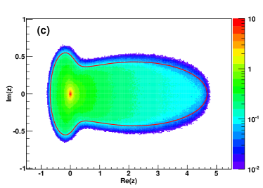
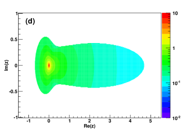
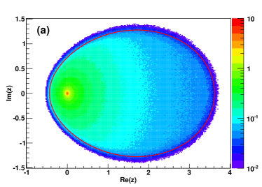
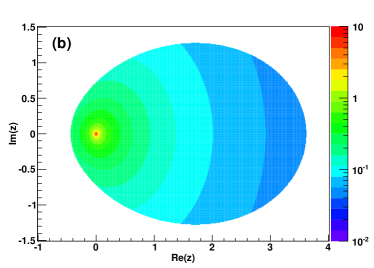
which may be solved for any value of ϕ[0,2π)italic-ϕ02𝜋\phi\in[0,2\pi) giving the desired contour. Then one may numerically solve the polynomial Eqs. (88,89) inside the eigenvalue domain. The results for different values of μ𝜇\mu, are presented in Fig. 5 supported by numerical simulation of random matrices. Theoretical predictions match the simulation up to finite size effects.
Refer to caption
Refer to caption
Refer to caption
Refer to caption
Refer to caption
Refer to caption
Figure 5: (Color online) Numerical eigenvalue distribution for matrices (𝟙+E1)(𝟙+E2)double-struck-𝟙subscript𝐸1double-struck-𝟙subscript𝐸2(\mathbb{1}+E_{1})(\mathbb{1}+E_{2}) 100×100100100100\times 100 for (a)μ=1/3𝜇13\mu=1/3 (c) μ=4/5𝜇45\mu=4/5 and (e) μ=23/25𝜇2325\mu=23/25 compared with theoretically evaluated ones in (b), (d) and (f) respectively. The edge of the distribution is shown on the plots (a), (c) and (e) (red curve). Each histogram is made from 107superscript10710^{7} eigenvalues.

Finally the last example to be analyzed here is the product of the form:

AB=(𝟙+H)(𝟙+X),𝐴𝐵double-struck-𝟙𝐻double-struck-𝟙𝑋AB=(\mathbb{1}+H)(\mathbb{1}+X), (92)

of a shifted standardized hermitian GUE matrix A=𝟙+H𝐴double-struck-𝟙𝐻A=\mathbb{1}+H and a shifted standardized Ginibre matrix B=𝟙+X𝐵double-struck-𝟙𝑋B=\mathbb{1}+X. The R transforms are special cases of the elliptic one (85), for μ=1𝜇1\mu=1 and μ=0𝜇0\mu=0 respectively. The calculation procedure is analogous to the previous ones. The R transform for the product is:

AB(𝒢AB)=(1+wBv¯AvBeiϕeiϕ/2(vA+wBvA+vBeiϕ)eiϕ/2(v¯A+w¯Bv¯A+v¯Beiϕ)1+w¯BvAv¯Beiϕ).subscript𝐴𝐵subscript𝒢𝐴𝐵1subscript𝑤𝐵subscript¯𝑣𝐴subscript𝑣𝐵superscript𝑒𝑖italic-ϕsuperscript𝑒𝑖italic-ϕ2subscript𝑣𝐴subscript𝑤𝐵subscript𝑣𝐴subscript𝑣𝐵superscript𝑒𝑖italic-ϕsuperscript𝑒𝑖italic-ϕ2subscript¯𝑣𝐴subscript¯𝑤𝐵subscript¯𝑣𝐴subscript¯𝑣𝐵superscript𝑒𝑖italic-ϕ1subscript¯𝑤𝐵subscript𝑣𝐴subscript¯𝑣𝐵superscript𝑒𝑖italic-ϕ\mathcal{R}_{AB}\left(\mathcal{G}_{AB}\right)=\left(\begin{array}[]{cc}1+w_{B}-\bar{v}_{A}v_{B}e^{i\phi}&e^{-i\phi/2}\left(v_{A}+w_{B}v_{A}+v_{B}e^{i\phi}\right)\\ -e^{i\phi/2}\left(\bar{v}_{A}+\bar{w}_{B}\bar{v}_{A}+\bar{v}_{B}e^{-i\phi}\right)&1+\bar{w}_{B}-v_{A}\bar{v}_{B}e^{-i\phi}\end{array}\right). (93)

The Green’s function reads

GAB(z)=subscript𝐺𝐴𝐵𝑧absent\displaystyle G_{AB}\left(z\right)= (94)
=1reiϕ+w¯BeiϕvAv¯B2Re(reiϕ(1+w¯B))(r2+(2Re(wB)+|wB|2)(1+|vA|2)+2rRe(vAv¯B)+(1+|vA|2)(1+|vB|2)).absent1𝑟superscript𝑒𝑖italic-ϕsubscript¯𝑤𝐵superscript𝑒𝑖italic-ϕsubscript𝑣𝐴subscript¯𝑣𝐵2Re𝑟superscript𝑒𝑖italic-ϕ1subscript¯𝑤𝐵superscript𝑟22Resubscript𝑤𝐵superscriptsubscript𝑤𝐵21superscriptsubscript𝑣𝐴22𝑟Resubscript𝑣𝐴subscript¯𝑣𝐵1superscriptsubscript𝑣𝐴21superscriptsubscript𝑣𝐵2\displaystyle=\frac{1-re^{-i\phi}+\bar{w}_{B}-e^{-i\phi}v_{A}\bar{v}_{B}}{2\mathrm{Re}\left(re^{i\phi}\left(1+\bar{w}_{B}\right)\right)-\left(r^{2}+\left(2\mathrm{Re}\left(w_{B}\right)+\left|w_{B}\right|^{2}\right)\left(1+\left|v_{A}\right|^{2}\right)+2r\mathrm{Re}\left(v_{A}\bar{v}_{B}\right)+\left(1+\left|v_{A}\right|^{2}\right)\left(1+\left|v_{B}\right|^{2}\right)\right)}. (95)

The solution vA=vB=0subscript𝑣𝐴subscript𝑣𝐵0v_{A}=v_{B}=0 again gives a holomorphic Green’s function. Then, in similar way to the previous two cases it is sufficient to consider linear terms to obtain eigenvalue domain. One is left with three independent equations relating wAsubscript𝑤𝐴w_{A}, wBsubscript𝑤𝐵w_{B}, r𝑟r and ϕitalic-ϕ\phi

r𝑟\displaystyle r =(1+wB+wB2)eiϕwB,absent1subscript𝑤𝐵superscriptsubscript𝑤𝐵2superscript𝑒𝑖italic-ϕsubscript𝑤𝐵\displaystyle=\frac{\left(1+w_{B}+w_{B}^{2}\right)e^{-i\phi}}{w_{B}}, (96)
wAsubscript𝑤𝐴\displaystyle w_{A} =wB(1+wB),absentsubscript𝑤𝐵1subscript𝑤𝐵\displaystyle=w_{B}\left(1+w_{B}\right), (97)
00\displaystyle 0 =1+|wB|2+wBe2iϕ(1+wB+w¯B).absent1superscriptsubscript𝑤𝐵2subscript𝑤𝐵superscript𝑒2𝑖italic-ϕ1subscript𝑤𝐵subscript¯𝑤𝐵\displaystyle=-1+\left|w_{B}\right|^{2}+w_{B}e^{2i\phi}\left(1+w_{B}+\bar{w}_{B}\right). (98)

It is pointless to give explicit solutions for w𝑤w’s, as they are given by long and cumbersome formulas. One can nevertheless implement them to a numerical code to evaluate the position r𝑟r of the density border for any ϕ[0,2π)italic-ϕ02𝜋\phi\in[0,2\pi) through Eq. (96). It turns out that the solution has two branches, each forming a closed loop around a different portion of the eigenvalue density. The loops touch at a single point at the origin z=0𝑧0z=0. The result and the comparison to numerical simulations for finite matrices is presented in Fig. 6. The finite N results based on the MC simulation converge to the theoretically evaluated domain while the size of matrix is being increased.
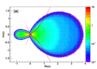
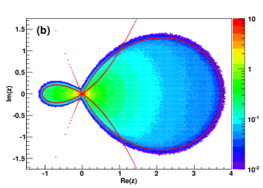
Refer to caption
Refer to caption
Refer to caption
Figure 6: (Color online) Numerical eigenvalue distribution for matrices (𝟙+H)(𝟙+X)double-struck-𝟙𝐻double-struck-𝟙𝑋(\mathbb{1}+H)(\mathbb{1}+X) of size (a) 50×50505050\times 50 (b) 100×100100100100\times 100 and (c) 200×200200200200\times 200 compared with theoretical prediction for the edge of the distribution (red points). Each histogram is made from 107superscript10710^{7} eigenvalues. The eigenvalue domain is determined by closed regions given by analytic solutions of Eqs. (96) and (98).

VII Conclusions

One can systematically define the Green’s function and the R transform for non-hermitian random matrices given by invariant measures of the form (44) and calculate the corresponding eigenvalue densities in the limit N𝑁N\rightarrow\infty. The Green’s function and the R transform have an analogous structure to those for hermitian matrices known from the standard free probability calculus, but they are quaternionic. We demonstrated how to derive these functions using the Cayley-Dickson construction.

The addition and multiplication laws for invariant non-hermitian matrices can be deduced from Feynman perturbation theory for matrix models with the invariant measures. These laws provide us with a practical method to calculate the limiting eigenvalue densities for sums and products of non-hermitian invariant random matrices in the limit N𝑁N\rightarrow\infty.

If one combines the method discussed in this paper with the trick of linearization gjjn ; hst one can also apply it to determine eigenvalue densities of more complicated matrix polynomials. So far this method could only be applied to polynomials which were hermitian by construction as for instance AB+BA+A+B𝐴𝐵𝐵𝐴𝐴𝐵AB+BA+A+B or ABC+BCA+CAB𝐴𝐵𝐶𝐵𝐶𝐴𝐶𝐴𝐵ABC+BCA+CAB for A𝐴A, B𝐵B and C𝐶C being hermitian. This required a special adaptation of the linearization method a ; bms . Now, this constraint can be removed and one can treat non-hermitian polynomials as well, as for instance AB+A+B𝐴𝐵𝐴𝐵AB+A+B or ABC+BCA𝐴𝐵𝐶𝐵𝐶𝐴ABC+BCA.

As mentioned before, the non-hermitian products of random matrices appear in multiple contexts including iterative stochastic evolution of linear systems n ; f ; abk , capacity of complicated MIMO networks mu ; awk or analysis of multi-dimensional data with asymmetric correlations, like e.g. time series of stock prices j ; bt ; blmp ; lr and others. Many of such problems were tackled with methods of free probability in the hermitian case. Now, by the use of the quaternionic R-transform, they can be extended towards the non-hermitian regime which is often computationally harder, but physically better motivated.

Acknowledgments

The work was supported by the Grant DEC-2011/02/A/ST1/00119 of the National Centre of Science and German Research Foundation via Collaborative Research Center/Transregio 12. The authors thank R. Janik, A. Jarosz and M.A. Nowak for discussions.

Appendix A

In this Appendix we recall the Cayley-Dickson construction of quaternions and discuss an extension of this construction to matrices.

Quaternions q𝑞q are linear combinations

q=a+bi+cj+dk𝑞𝑎𝑏𝑖𝑐𝑗𝑑𝑘q=a+bi+cj+dk (99)

of quaternionic units 1,i,j,k1𝑖𝑗𝑘1,i,j,k with real coefficients a,b,c,d𝑎𝑏𝑐𝑑a,b,c,d. The quaternionic units form the Hamilton basis which is defined by the the following multiplication rules

i2=j2=k2=ijk=1.superscript𝑖2superscript𝑗2superscript𝑘2𝑖𝑗𝑘1i^{2}=j^{2}=k^{2}=ijk=-1\ . (100)

Quaternions can be represented as ordered pairs (z,w)𝑧𝑤(z,w) of complex numbers z=a+bi𝑧𝑎𝑏𝑖z=a+bi, w=c+di𝑤𝑐𝑑𝑖w=c+di

q=a+bi+(c+di)j=z+wj(z,w).𝑞𝑎𝑏𝑖𝑐𝑑𝑖𝑗𝑧𝑤𝑗𝑧𝑤q=a+bi+(c+di)j=z+wj\equiv(z,w)\ . (101)

The conjugate of q𝑞q is q=abicjdk=z¯wj=(z¯,w)superscript𝑞𝑎𝑏𝑖𝑐𝑗𝑑𝑘¯𝑧𝑤𝑗¯𝑧𝑤q^{*}=a-bi-cj-dk=\bar{z}-wj=(\bar{z},-w). Quaternion addition is defined by

(z,w)+(v,y)=(z+v,w+y),𝑧𝑤𝑣𝑦𝑧𝑣𝑤𝑦(z,w)+(v,y)=(z+v,w+y)\ , (102)

and multiplication by

(z,w)(v,y)=(zvwy¯,zy+wv¯).𝑧𝑤𝑣𝑦𝑧𝑣𝑤¯𝑦𝑧𝑦𝑤¯𝑣(z,w)(v,y)=(zv-w\bar{y},zy+w\bar{v})\ . (103)

It is useful to define auxiliary functions F𝐹F and S𝑆S which allow one to extract the first and the second element of the Cayley-Dickson pair q=(z,w)𝑞𝑧𝑤q=(z,w)

z=F(q),w=S(q).formulae-sequence𝑧𝐹𝑞𝑤𝑆𝑞z=F(q)\ ,\ w=S(q)\ . (104)

These functions play an analogous role for quaternions as the real and imaginary parts for complex numbers. We refer to them as to ”first part” and ”second part” of quaternion. Quaternions have a matrix representation in terms of Pauli matrices σisubscript𝜎𝑖\sigma_{i}. A quaternion q=a+bi+cj+dk=(z,w)𝑞𝑎𝑏𝑖𝑐𝑗𝑑𝑘𝑧𝑤q=a+bi+cj+dk=(z,w) can be mapped to two-by-two complex matrix (we use the same letter to denote this matrix) by

q=aσ0+b(iσ3)+c(iσ2)+d(iσ1)=(a+ibc+idc+idaib)=(zww¯z¯).𝑞𝑎subscript𝜎0𝑏𝑖subscript𝜎3𝑐𝑖subscript𝜎2𝑑𝑖subscript𝜎1𝑎𝑖𝑏𝑐𝑖𝑑𝑐𝑖𝑑𝑎𝑖𝑏𝑧𝑤¯𝑤¯𝑧q=a\sigma_{0}+b(i\sigma_{3})+c(i\sigma_{2})+d(i\sigma_{1})=\left(\begin{array}[]{cc}a+ib&c+id\\ -c+id&a-ib\end{array}\right)=\left(\begin{array}[]{cc}z&w\\ -\bar{w}&\bar{z}\end{array}\right)\ . (105)

The first row of the quaternion matrix representation (105) can be identified with the Cayley-Dickson pair (z,w)𝑧𝑤(z,w). It is easy to check that the matrices σ0,iσ3,iσ2,iσ1subscript𝜎0𝑖subscript𝜎3𝑖subscript𝜎2𝑖subscript𝜎1\sigma_{0},i\sigma_{3},i\sigma_{2},i\sigma_{1} form the Hamilton basis (100)

(iσ3)2=(iσ2)2=(iσ1)2=(iσ3)(iσ2)(iσ1)=σ0.superscript𝑖subscript𝜎32superscript𝑖subscript𝜎22superscript𝑖subscript𝜎12𝑖subscript𝜎3𝑖subscript𝜎2𝑖subscript𝜎1subscript𝜎0(i\sigma_{3})^{2}=(i\sigma_{2})^{2}=(i\sigma_{1})^{2}=(i\sigma_{3})(i\sigma_{2})(i\sigma_{1})=-\sigma_{0}\ . (106)

Quaternion addition corresponds in this representation to matrix addition while quaternion multiplication to matrix multiplication:

(zww¯z¯)(vyy¯v¯)=(zvwy¯zy+wv¯z¯y¯w¯vz¯v¯w¯y)𝑧𝑤¯𝑤¯𝑧𝑣𝑦¯𝑦¯𝑣𝑧𝑣𝑤¯𝑦𝑧𝑦𝑤¯𝑣¯𝑧¯𝑦¯𝑤𝑣¯𝑧¯𝑣¯𝑤𝑦\left(\begin{array}[]{cc}z&w\\ -\bar{w}&\bar{z}\end{array}\right)\left(\begin{array}[]{cc}v&y\\ -\bar{y}&\bar{v}\end{array}\right)=\left(\begin{array}[]{cc}zv-w\bar{y}&zy+w\bar{v}\\ -\bar{z}\bar{y}-\bar{w}v&\bar{z}\bar{v}-\bar{w}y\end{array}\right) (107)

as can be seen by comparing the upper rows of matrices in the last equation with the Cayley-Dickson pairs in (103). The conjugate quaternion corresponds to the hermitian conjugate q=qsuperscript𝑞superscript𝑞q^{*}=q^{\dagger}. The quaternion norm squared is q2=qq=detqsuperscriptnorm𝑞2𝑞superscript𝑞𝑞||q||^{2}=qq^{\dagger}=\det q and the inverse quaternion q1=q/detqsuperscript𝑞1superscript𝑞𝑞q^{-1}=q^{\dagger}/\det q.

We now superimpose the quaternionic structure on N×N𝑁𝑁N\times N matrices. Given four hermitian N×N𝑁𝑁N\times N matrices A,B,C,D𝐴𝐵𝐶𝐷A,B,C,D we construct two non-hermitian matrices X=A+iB𝑋𝐴𝑖𝐵X=A+iB and Y=C+iD𝑌𝐶𝑖𝐷Y=C+iD and a 2N×2N2𝑁2𝑁2N\times 2N quaternionic matrix

𝒬=Aσ0+Biσ3+Ciσ2+Diσ1=(A+iBC+iDC+iDAiB)=(XYYX)(X,Y).𝒬tensor-product𝐴subscript𝜎0tensor-product𝐵𝑖subscript𝜎3tensor-product𝐶𝑖subscript𝜎2tensor-product𝐷𝑖subscript𝜎1𝐴𝑖𝐵𝐶𝑖𝐷𝐶𝑖𝐷𝐴𝑖𝐵𝑋𝑌superscript𝑌superscript𝑋𝑋𝑌\mathcal{Q}=A\otimes\sigma_{0}+B\otimes i\sigma_{3}+C\otimes i\sigma_{2}+D\otimes i\sigma_{1}=\left(\begin{array}[]{cc}A+iB&C+iD\\ -C+iD&A-iB\end{array}\right)=\left(\begin{array}[]{cc}X&Y\\ -Y^{\dagger}&X^{\dagger}\end{array}\right)\equiv(X,Y)\ . (108)

The upper row of blocks specify the whole matrix, so we can use the notation 𝒬=(X,Y)𝒬𝑋𝑌\mathcal{Q}=(X,Y) is as in the Cayley-Dickson construction. As before, we define the functions F𝐹F and S𝑆S to extract the first and the second block of the pair

X=F(𝒬),Y=S(𝒬).formulae-sequence𝑋𝐹𝒬𝑌𝑆𝒬X=F({\cal Q})\ ,\ Y=S({\cal Q})\ . (109)

Additionally we denote a trace in space of quaternionic matrices, which acts as block-trace operation in Pauli matrix representation, by Trb𝒬=(TrX,TrY)subscriptTrb𝒬Tr𝑋Tr𝑌\mathrm{Tr_{b}}\mathcal{Q}=(\mathrm{Tr}X,\mathrm{Tr}Y). It projects quaternionic matrices to quaternions

Trb𝒬=(TrXTrYTrYTrX).subscriptTrb𝒬Tr𝑋Tr𝑌Trsuperscript𝑌Trsuperscript𝑋\mathrm{Tr_{b}}\mathcal{Q}=\left(\begin{array}[]{cc}\mathrm{Tr}X&\mathrm{Tr}Y\\ -\mathrm{Tr}Y^{\dagger}&\mathrm{Tr}X^{\dagger}\end{array}\right)\ . (110)

Equipped with this matrix extension of quaternions one can naturally define pertinent objects to handle non-hermitian matrices including the quaternionic resolvent and the R transform.

Appendix B

We show here that Eq. (5) can be treated as a representation of the two-dimensional delta function. We have

1πz¯F1z+wj=1πz¯Fz¯wj|z|2+|w|2=1πz¯z¯|z|2+|w|2=1π|w|2(|z|2+|w|2)2.1𝜋¯𝑧𝐹1𝑧𝑤𝑗1𝜋¯𝑧𝐹¯𝑧𝑤𝑗superscript𝑧2superscript𝑤21𝜋¯𝑧¯𝑧superscript𝑧2superscript𝑤21𝜋superscript𝑤2superscriptsuperscript𝑧2superscript𝑤22\frac{1}{\pi}\frac{\partial}{\partial\bar{z}}F\frac{1}{z+wj}=\frac{1}{\pi}\frac{\partial}{\partial\bar{z}}F\frac{\bar{z}-wj}{|z|^{2}+|w|^{2}}=\frac{1}{\pi}\frac{\partial}{\partial\bar{z}}\frac{\bar{z}}{|z|^{2}+|w|^{2}}=\frac{1}{\pi}\frac{|w|^{2}}{\left(\left|z\right|^{2}+|w|^{2}\right)^{2}}\ . (111)

The resulting function is a circularly symmetric bell-shaped function located at the origin of the z𝑧z-complex plane. The width of the peak at half maximum is of order |w|𝑤|w| and the height of order 1/|w|21superscript𝑤21/|w|^{2}. For any non-zero value of w𝑤w the integral of this function over the whole z𝑧z-complex plane is equal one

1π|w|2(|z|2+|w|2)2d2z=1.1𝜋superscript𝑤2superscriptsuperscript𝑧2superscript𝑤22superscript𝑑2𝑧1\int\frac{1}{\pi}\frac{|w|^{2}}{\left(\left|z\right|^{2}+|w|^{2}\right)^{2}}d^{2}z=1\ . (112)

and it is independent of w𝑤w. In the limit w0𝑤0w\rightarrow 0 the volume under the peak stays constant while the width of the peak tends to zero. The whole function and its integral gets concentrated in a single point so it is the delta function.

We note that also the second part of the inverse quaternion can be used to define the two-dimensional Dirac delta

1πw¯S1z+wj=1πw¯w|z|2+|w|2=ww¯1π|w|2(|z|2+|w|2)2.1𝜋¯𝑤𝑆1𝑧𝑤𝑗1𝜋¯𝑤𝑤superscript𝑧2superscript𝑤2𝑤¯𝑤1𝜋superscript𝑤2superscriptsuperscript𝑧2superscript𝑤22\frac{1}{\pi}\frac{\partial}{\partial\bar{w}}S\frac{1}{z+wj}=-\frac{1}{\pi}\frac{\partial}{\partial\bar{w}}\frac{w}{|z|^{2}+|w|^{2}}=\frac{w}{\bar{w}}\frac{1}{\pi}\frac{|w|^{2}}{\left(\left|z\right|^{2}+|w|^{2}\right)^{2}}\ . (113)

We see that when we fix the argument ϕitalic-ϕ\phi of w=eiϕ|w|𝑤superscript𝑒𝑖italic-ϕ𝑤w=e^{i\phi}|w| and take the limit |w|0+𝑤superscript0|w|\rightarrow 0^{+} we obtain the delta function multiplied by a phase factor e2iϕδ(2)(z)superscript𝑒2𝑖italic-ϕsuperscript𝛿2𝑧e^{2i\phi}\delta^{(2)}(z). For ϕ=0italic-ϕ0\phi=0 this expression reduces to the delta function. This representation is closer in spirit to the standard representation of the one-dimensional delta (4) since the second part S𝑆S for quaternions is like the imaginary part m𝑚\Im m for complex numbers. This representation is however more difficult to use in practice since one has to extract the dependence on w𝑤w and calculate the derivative before one takes the limit.

Appendix C

One can show fs2 that the expression in the brackets in Eq. (11) behaves in the limit w0𝑤0w\rightarrow 0 as a sum of delta functions located at eigenvalues of X𝑋X

limN1NTrHR1|w|2HL11Ni=1Nδ(2)(zλi).subscript𝑁1𝑁Trsuperscriptsubscript𝐻𝑅1superscript𝑤2superscriptsubscript𝐻𝐿11𝑁superscriptsubscript𝑖1𝑁superscript𝛿2𝑧subscript𝜆𝑖\lim_{N\rightarrow\infty}\frac{1}{N}\mathrm{Tr}H_{R}^{-1}|w|^{2}H_{L}^{-1}\longrightarrow\frac{1}{N}\sum_{i=1}^{N}\delta^{(2)}\left(z-\lambda_{i}\right)\ . (114)

We repeat this reasoning here. The two matrices HLsubscript𝐻𝐿H_{L} and HRsubscript𝐻𝑅H_{R} (9) are hermitian, therefore they have real eigenvalues. We assume that they are non-degenerate. Denote the corresponding eigenvectors by |Lαketsubscript𝐿𝛼|L_{\alpha}\rangle and |Rαketsubscript𝑅𝛼|R_{\alpha}\rangle respectively

HL|Lα=Λα|LαHR|Rα=Λα|Rα.subscript𝐻𝐿ketsubscript𝐿𝛼subscriptΛ𝛼ketsubscript𝐿𝛼subscript𝐻𝑅ketsubscript𝑅𝛼subscriptΛ𝛼ketsubscript𝑅𝛼\begin{split}H_{L}|L_{\alpha}\rangle&=\Lambda_{\alpha}|L_{\alpha}\rangle\\ H_{R}|R_{\alpha}\rangle&=\Lambda_{\alpha}|R_{\alpha}\rangle\ .\end{split} (115)

The two matrices have the same eigenvalues. Indeed, multiplying the first equation on both sides by (z¯𝟙X)¯𝑧double-struck-𝟙superscript𝑋(\bar{z}\mathbb{1}-X^{\dagger}) and using the identity (z¯𝟙X)HL=HR(z¯𝟙X)¯𝑧double-struck-𝟙superscript𝑋subscript𝐻𝐿subscript𝐻𝑅¯𝑧double-struck-𝟙superscript𝑋(\bar{z}\mathbb{1}-X^{\dagger})H_{L}=H_{R}(\bar{z}\mathbb{1}-X^{\dagger}) we get

HR(z¯𝟙X)|Lα=Λα(z¯𝟙X)|Lα,subscript𝐻𝑅¯𝑧double-struck-𝟙superscript𝑋ketsubscript𝐿𝛼subscriptΛ𝛼¯𝑧double-struck-𝟙superscript𝑋ketsubscript𝐿𝛼H_{R}(\bar{z}\mathbb{1}-X^{\dagger})|L_{\alpha}\rangle=\Lambda_{\alpha}(\bar{z}\mathbb{1}-X^{\dagger})|L_{\alpha}\rangle\ , (116)

which means that |Rα=η(z¯𝟙X)|Lαketsubscript𝑅𝛼𝜂¯𝑧double-struck-𝟙superscript𝑋ketsubscript𝐿𝛼|R_{\alpha}\rangle=\eta(\bar{z}\mathbb{1}-X^{\dagger})|L_{\alpha}\rangle is an eigenvector of HRsubscript𝐻𝑅H_{R} to the same eigenvalue ΛαsubscriptΛ𝛼\Lambda_{\alpha}. The coefficient η𝜂\eta is to fix the norm of the vector Rα|Rα=1inner-productsubscript𝑅𝛼subscript𝑅𝛼1\langle R_{\alpha}|R_{\alpha}\rangle=1. Using the spectral decomposition of HLsubscript𝐻𝐿H_{L} and HRsubscript𝐻𝑅H_{R} one can cast the expression on the left hand side of Eq. (114) into the form

1NTrHR1|w|2HL1=1Nα=1Nβ=1N|w|2|Rα|Lβ|2ΛαΛβ.1𝑁Trsuperscriptsubscript𝐻𝑅1superscript𝑤2superscriptsubscript𝐻𝐿11𝑁superscriptsubscript𝛼1𝑁superscriptsubscript𝛽1𝑁superscript𝑤2superscriptinner-productsubscript𝑅𝛼subscript𝐿𝛽2subscriptΛ𝛼subscriptΛ𝛽\frac{1}{N}\mathrm{Tr}H_{R}^{-1}|w|^{2}H_{L}^{-1}=\frac{1}{N}\sum_{\alpha=1}^{N}\sum_{\beta=1}^{N}\frac{|w|^{2}\left|\langle R_{\alpha}|L_{\beta}\rangle\right|^{2}}{\Lambda_{\alpha}\Lambda_{\beta}}\ . (117)

The eigenvalues ΛαsubscriptΛ𝛼\Lambda_{\alpha} and eigenvectors |Rαketsubscript𝑅𝛼|R_{\alpha}\rangle and |Lαketsubscript𝐿𝛼|L_{\alpha}\rangle depend on X𝑋X but also on w𝑤w and z𝑧z. In our notation this dependence is implicit. We will display it if needed. When z𝑧z is not equal to an eigenvalue of X𝑋X the eigenvalues Λα(z,w=0)subscriptΛ𝛼𝑧𝑤0\Lambda_{\alpha}(z,w=0) of HLsubscript𝐻𝐿H_{L} and HRsubscript𝐻𝑅H_{R} (9) are strictly positive. As a consequence the expression on the right hand side of Eq. (117) behaves as |w|2superscript𝑤2|w|^{2} for small w𝑤w and vanishes for w=0𝑤0w=0. The situation changes when z𝑧z is equal to an eigenvalue of X𝑋X because in this case the smallest eigenvalue Λ0(z=λj,w)=|w|2subscriptΛ0𝑧subscript𝜆𝑗𝑤superscript𝑤2\Lambda_{0}(z=\lambda_{j},w)=|w|^{2} of HLsubscript𝐻𝐿H_{L} and HRsubscript𝐻𝑅H_{R} tends to zero for w0𝑤0w\rightarrow 0 and then the expression (117) diverges as 1/|w|21superscript𝑤21/|w|^{2}

1NTrHR1|w|2HL1|R0|L0|2|w|2.proportional-to1𝑁Trsuperscriptsubscript𝐻𝑅1superscript𝑤2superscriptsubscript𝐻𝐿1superscriptinner-productsubscript𝑅0subscript𝐿02superscript𝑤2\frac{1}{N}\mathrm{Tr}H_{R}^{-1}|w|^{2}H_{L}^{-1}\propto\frac{\left|\langle R_{0}|L_{0}\rangle\right|^{2}}{|w|^{2}}\ . (118)

The divergence comes from the term α=β=0𝛼𝛽0\alpha=\beta=0 of the sum (117). To summarize, in the limit w0𝑤0w\rightarrow 0 the expression on the left hand side of Eq. (114) vanishes for all values of z𝑧z except those equal to eigenvalues of X𝑋X. A more careful analysis of the behavior of the expression (117) in the vicinity of eigenvalues of X𝑋X shows that it behaves as delta functions located at those eigenvalues. In order to see this consider z𝑧z close to an eigenvalue λjsubscript𝜆𝑗\lambda_{j} of X𝑋X: such that the distance |zλj|𝑧subscript𝜆𝑗|z-\lambda_{j}| is much smaller than the eigenvalue separation. One can apply the perturbation theory to determine the lowest eigenvalue of HLsubscript𝐻𝐿H_{L} and HRsubscript𝐻𝑅H_{R} (9). Up to the second order one finds

Λ0|w|2+|R0|L0|2|zλj|2.subscriptΛ0superscript𝑤2superscriptinner-productsubscript𝑅0subscript𝐿02superscript𝑧subscript𝜆𝑗2\Lambda_{0}\approx|w|^{2}+\left|\langle R_{0}|L_{0}\rangle\right|^{2}|z-\lambda_{j}|^{2}\ . (119)

Inserting Λ0subscriptΛ0\Lambda_{0} to the diverging term (α=β=0𝛼𝛽0\alpha=\beta=0) of the sum (117) and neglecting remaining terms, which are of order |w|0superscript𝑤0|w|^{0} or |w|2superscript𝑤2|w|^{2}, one finds for w0𝑤0w\rightarrow 0

1NTrHR1|w|2HL11N|w|2|R0|L0|2(|w|2+|R0|L0|2|zλj|2)21Nδ(2)(zλj).1𝑁Trsuperscriptsubscript𝐻𝑅1superscript𝑤2superscriptsubscript𝐻𝐿11𝑁superscript𝑤2superscriptinner-productsubscript𝑅0subscript𝐿02superscriptsuperscript𝑤2superscriptinner-productsubscript𝑅0subscript𝐿02superscript𝑧subscript𝜆𝑗221𝑁superscript𝛿2𝑧subscript𝜆𝑗\frac{1}{N}\mathrm{Tr}H_{R}^{-1}|w|^{2}H_{L}^{-1}\approx\frac{1}{N}\frac{|w|^{2}\left|\langle R_{0}|L_{0}\rangle\right|^{2}}{\left(|w|^{2}+\left|\langle R_{0}|L_{0}\rangle\right|^{2}|z-\lambda_{j}|^{2}\right)^{2}}\longrightarrow\frac{1}{N}\delta^{(2)}(z-\lambda_{j})\ . (120)

The same holds for z𝑧z in the vicinity of any eigenvalue λisubscript𝜆𝑖\lambda_{i} of X𝑋X so one eventually arrives at Eq. (114).

Appendix D

In this appendix we recall diagrammatic derivation of Eqs. (15) and (28). We begin with hermitian matrices and towards the end we describe how to generalize the derivation to non-hermitian ones.

Let us recall main ideas bipz ; biz and introduce graphical notation. We consider hermitian random matrices defined by the probability measure

dμ(H)DHexpNTrV(H)=DHexpNTr(12H2+g33H3+g44H4+),proportional-to𝑑𝜇𝐻𝐷𝐻𝑁Tr𝑉𝐻𝐷𝐻𝑁Tr12superscript𝐻2subscript𝑔33superscript𝐻3subscript𝑔44superscript𝐻4d\mu(H)\propto DH\exp-N\mathrm{Tr}V(H)=DH\exp-N\mathrm{Tr}\left(\frac{1}{2}H^{2}+\frac{g_{3}}{3}H^{3}+\frac{g_{4}}{4}H^{4}+\ldots\right)\ , (121)

and apply Gaussian perturbation theory to calculate statistical averages delimited-⟨⟩\langle\ldots\rangle with respect to this measure. One does it by spliting the measure into the Gaussian part and the residual part V(H)=12H2+VR(H)𝑉𝐻12superscript𝐻2subscript𝑉𝑅𝐻V(H)=\frac{1}{2}H^{2}+V_{R}(H), where VR(H)=g33H3+g44H4+subscript𝑉𝑅𝐻subscript𝑔33superscript𝐻3subscript𝑔44superscript𝐻4V_{R}(H)=\frac{g_{3}}{3}H^{3}+\frac{g_{4}}{4}H^{4}+\ldots, and treating the latter as a perturbation

dμ(H)=dμ0(H)(1+NTrVR(H)+12(NTrVR(H))2+),𝑑𝜇𝐻𝑑subscript𝜇0𝐻1𝑁Trsubscript𝑉𝑅𝐻12superscript𝑁Trsubscript𝑉𝑅𝐻2d\mu(H)=d\mu_{0}(H)\left(1+N\mathrm{Tr}V_{R}(H)+\frac{1}{2}\left(N\mathrm{Tr}V_{R}(H)\right)^{2}+\ldots\right)\ , (122)

where dμ0(H)expNTrH2/2proportional-to𝑑subscript𝜇0𝐻𝑁Trsuperscript𝐻22d\mu_{0}(H)\propto\exp-N\mathrm{Tr}H^{2}/2 with a normalization ensuring that 𝑑μ0(H)=1differential-dsubscript𝜇0𝐻1\int d\mu_{0}(H)=1. Now the problem reduces to calculating averages of powers of H𝐻H with respect to the Gaussian measure 0=𝑑μ0(H)subscriptdelimited-⟨⟩0differential-dsubscript𝜇0𝐻\langle\ldots\rangle_{0}=\int d\mu_{0}(H)\ldots. As follows from the Wick’s theorem, averages with respect to the Gaussian measure of higher order products of H𝐻H can be replaced by products of the averages of second order products. For example for the fourth order the theorem tells us that

HabHcdHefHgh0=HabHcd0HefHgh0+HabHef0HcdHgh0+HabHgh0HefHcd0.subscriptdelimited-⟨⟩subscript𝐻𝑎𝑏subscript𝐻𝑐𝑑subscript𝐻𝑒𝑓subscript𝐻𝑔0subscriptdelimited-⟨⟩subscript𝐻𝑎𝑏subscript𝐻𝑐𝑑0subscriptdelimited-⟨⟩subscript𝐻𝑒𝑓subscript𝐻𝑔0subscriptdelimited-⟨⟩subscript𝐻𝑎𝑏subscript𝐻𝑒𝑓0subscriptdelimited-⟨⟩subscript𝐻𝑐𝑑subscript𝐻𝑔0subscriptdelimited-⟨⟩subscript𝐻𝑎𝑏subscript𝐻𝑔0subscriptdelimited-⟨⟩subscript𝐻𝑒𝑓subscript𝐻𝑐𝑑0\langle H_{ab}H_{cd}H_{ef}H_{gh}\rangle_{0}=\langle H_{ab}H_{cd}\rangle_{0}\langle H_{ef}H_{gh}\rangle_{0}+\langle H_{ab}H_{ef}\rangle_{0}\langle H_{cd}H_{gh}\rangle_{0}+\langle H_{ab}H_{gh}\rangle_{0}\langle H_{ef}H_{cd}\rangle_{0}\ . (123)

This observation underlies the idea of Feynman diagrams which are just graphical representation of products of factors HabHcd0subscriptdelimited-⟨⟩subscript𝐻𝑎𝑏subscript𝐻𝑐𝑑0\langle H_{ab}H_{cd}\rangle_{0}. These factors are called propagators and are graphically represented as double lines between pairs of indices ab𝑎𝑏ab and cd𝑐𝑑cd as shown in Fig. 7a. It is easy to find, by doing the Guassian integral, that the numerical value of the propagator for dμ0(H)expNTrH2/2proportional-to𝑑subscript𝜇0𝐻𝑁Trsuperscript𝐻22d\mu_{0}(H)\propto\exp-N\mathrm{Tr}H^{2}/2 is

HabHcd0=1Nδadδbc.subscriptdelimited-⟨⟩subscript𝐻𝑎𝑏subscript𝐻𝑐𝑑01𝑁subscript𝛿𝑎𝑑subscript𝛿𝑏𝑐\langle H_{ab}H_{cd}\rangle_{0}=\frac{1}{N}\delta_{ad}\delta_{bc}\ . (124)
Refer to caption
Refer to caption
Refer to caption
Figure 7: Pictorial representation of the (a) propagator (124) and (b,c) the first two vertices generated by the perturbative expansion (122). In this appendix we use convention that external vertices are represented by open circles. In contrast, internal vertices (see below) are represented by filled circles. Internal vertices correspond to indices which are summed over.

This means that the only non-zero contributions of propagators are 1/N1𝑁1/N for a𝑎a equal to d𝑑d and c𝑐c to b𝑏b. Feynman diagrams are obtained by connecting vertices (see Fig. 7b,c) generated by perturbative expansion of the residual part VR(H)subscript𝑉𝑅𝐻V_{R}(H) (122) with lines representing propagators (124). An example of a diagram is shown in Fig. 8.
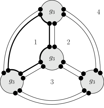
Refer to caption
Figure 8: Example of a planar Feynman diagram obtained from V=4𝑉4V=4 cubic vertices and E=6𝐸6E=6 propagators. It has F=4𝐹4F=4 closed lines, like e.g. the thick one surrounding the region 111. With each such closed line one can associate a face of polyhedron constructed from the edges of the diagram. If the diagram is drawn on a sphere, the region 444 can be viewed as a compact region or the fourth face of tetrahedron.

A contribution of the diagram to the perturbative expansion is given by a product of contributions from propagators and vertices. Propagators contribute (124) and vertices: Ng3/3𝑁subscript𝑔33Ng_{3}/3 and Ng4/4𝑁subscript𝑔44Ng_{4}/4 etc. The factor N𝑁N comes from the prefactor before trace (122). Let us concentrate on counting powers of N𝑁N for a given diagram. Each propagator contributes a factor 1/N1𝑁1/N (124), each vertex contributes a factor N𝑁N and each closed line, like the thick one drawn in Fig. 8, contributes a factor N𝑁N. This is because the summation over internal indices of delta functions (124) gives for a closed line a factor aδaa=Nsubscript𝑎subscript𝛿𝑎𝑎𝑁\sum_{a}\delta_{aa}=N. Such a closed line can be viewed as a face of polyhedron made of edges (double lines) of the given diagram. The total power is thus NV+FEsuperscript𝑁𝑉𝐹𝐸N^{V+F-E} where V𝑉V is the number of vertices, F𝐹F is the number of faces of the diagram viewed as polyhedron and E𝐸E is the number of edges (represented us double lines). The combination V+FE𝑉𝐹𝐸V+F-E is the Euler characteristic of the polyhedron or equivalently of a two-dimensional surface on which the diagram can be drawn without edge-crossing. In the example shown in Fig. 8 we have V=4𝑉4V=4, F=4𝐹4F=4 and E=6𝐸6E=6 and V+FE=2𝑉𝐹𝐸2V+F-E=2. This is equal to the Euler characteristic of sphere. Generally, V+FE=22h𝑉𝐹𝐸22V+F-E=2-2h, where hh is the genus of two-dimensional surface on which diagram can be drawn without crossings. h=00h=0 for sphere, h=11h=1 for torus, h=22h=2 for double torus, etc. Thus one can see that the leading contribution comes from planar diagrams, which can be drawn on sphere (or equivalently plane) without edge-crossing. Those which can be drawn on torus without edge-crossing are suppressed with 1/N21superscript𝑁21/N^{2} factor, on double torus with 1/N41superscript𝑁41/N^{4} etc. The diagrams which can be drawn on torus without edge-crossing can also be drawn on plane but then they have at least one edge-crossing. In Fig. 9 we show examples of lowest order diagrams which are planar (h=00h=0) and non-planar (h=11h=1). One can generalize this classification to diagrams with external lines by considering two-dimensional surfaces with boundaries.

The main conclusion is that in the limit N𝑁N\rightarrow\infty one can neglect contributions from non-planar diagrams which are suppressed with 1/N2h1superscript𝑁21/N^{2h} powers as compared to the leading contribution coming from planar diagrams. In effect, in this limit one can restrict enumeration only to planar diagrams. This observation was first made in th and the technique of planar diagram enumeration was developed in bipz ; biz .

Refer to caption

,   Refer to caption

Figure 9: Examples of (a) a planar diagram and (b) a non-planar one.

So let us recall the idea of graphical enumeration of planar diagrams. Denote the n𝑛n-point correlation function

(m^n)i1j1,,injn=Hi1j1Hi2j2Hinjnsubscriptsubscript^𝑚𝑛subscript𝑖1subscript𝑗1subscript𝑖𝑛subscript𝑗𝑛delimited-⟨⟩subscript𝐻subscript𝑖1subscript𝑗1subscript𝐻subscript𝑖2subscript𝑗2subscript𝐻subscript𝑖𝑛subscript𝑗𝑛\left(\widehat{m}_{n}\right)_{i_{1}j_{1},\ldots,i_{n}j_{n}}=\left\langle H_{i_{1}j_{1}}H_{i_{2}j_{2}}\ldots H_{i_{n}j_{n}}\right\rangle (125)

by a blob with n𝑛n-external double legs as in Fig. 10a.

Refer to caption

,    Refer to caption

Figure 10: Pictorial representation of (a) n𝑛n-point correlation function m^nsubscript^𝑚𝑛\widehat{m}_{n} and (b) n𝑛n-point connected correlation function κ^nsubscript^𝜅𝑛\widehat{\kappa}_{n}.

In perturbation theory the n𝑛n-point correlation function is calculated as a sum over all planar Feynman diagrams with n𝑛n external legs. An example of a diagram generated by the 444-point correlation function is shown in Fig. 11a.
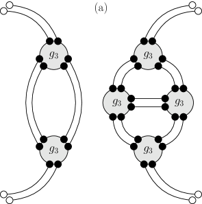
Refer to caption

,    Refer to caption

Figure 11: Examples of diagrams contributing to 444-point correlation function. The diagram (b) contributes to 444-point connected correlation function.

One also defines an n𝑛n-point connected correlation function which generates only connected diagrams with n𝑛n external legs. We denote it by

(κ^n)i1j1,injn=Hi1j1Hi2j2Hinjnsubscriptsubscript^𝜅𝑛subscript𝑖1subscript𝑗1subscript𝑖𝑛subscript𝑗𝑛delimited-⟨⟩delimited-⟨⟩subscript𝐻subscript𝑖1subscript𝑗1subscript𝐻subscript𝑖2subscript𝑗2subscript𝐻subscript𝑖𝑛subscript𝑗𝑛(\widehat{\kappa}_{n})_{i_{1}j_{1}\ldots,i_{n}j_{n}}=\langle\langle H_{i_{1}j_{1}}H_{i_{2}j_{2}}\ldots H_{i_{n}j_{n}}\rangle\rangle (126)

and in the graphical representation by a blob surrounded by a double contour (Fig. 10b). An example of a diagram generated by the 444-point connected correlation function is shown in Fig. 11b. Below we show how to use these functions in calculations of the Green’s function (2). It is useful to consider a generalized resolvent which is an N×N𝑁𝑁N\times N matrix of the form

G^=(Z^H)1,^𝐺delimited-⟨⟩superscript^𝑍𝐻1\widehat{G}=\left\langle\left(\widehat{Z}-H\right)^{-1}\right\rangle\ , (127)

where the matrix Z^^𝑍\widehat{Z} is an arbitrary invertible constant hermitian matrix. Clearly, by taking the normalized trace

G=limN1NTrG^𝐺subscript𝑁1𝑁Tr^𝐺G=\lim_{N\rightarrow\infty}\frac{1}{N}\mathrm{Tr}\;\widehat{G} (128)

and setting Z^=z𝟙^𝑍𝑧double-struck-𝟙\widehat{Z}=z\mathbb{1} one obtains the resolvent G(z)𝐺𝑧G(z) (2). We will set Z^=z𝟙^𝑍𝑧double-struck-𝟙\widehat{Z}=z\mathbb{1} only at the end of the calculations, while they will be done for an arbitrary Z^^𝑍\widehat{Z} in order to keep track of the underlying algebraic structure. Writing the resolvent (127) as a geometrical series one has

G^=(Z^H)1=Z^1+Z^1HZ^1+Z^1HZ^1HZ^1+.^𝐺delimited-⟨⟩superscript^𝑍𝐻1superscript^𝑍1delimited-⟨⟩superscript^𝑍1𝐻superscript^𝑍1delimited-⟨⟩superscript^𝑍1𝐻superscript^𝑍1𝐻superscript^𝑍1\widehat{G}=\left\langle(\widehat{Z}-H)^{-1}\right\rangle=\widehat{Z}^{-1}+\left\langle\widehat{Z}^{-1}H\widehat{Z}^{-1}\right\rangle+\left\langle\widehat{Z}^{-1}H\widehat{Z}^{-1}H\widehat{Z}^{-1}\right\rangle+\ldots\ . (129)

The factors depending on Z^^𝑍\widehat{Z} can be written outside the brackets since Z^^𝑍\widehat{Z} is a constant matrix. What remains in the brackets are n𝑛n-point correlation functions. For example, the contribution of the third term in the last equation to the matrix element G^afsubscript^𝐺𝑎𝑓\widehat{G}_{af} reads

(Z^1HZ^1HZ^1)af=b,c,d,eZ^ab1HbcZ^cd1HdeZ^ef1=b,c,d,eZ^ab1Z^cd1Z^ef1HbcHde.delimited-⟨⟩subscriptsuperscript^𝑍1𝐻superscript^𝑍1𝐻superscript^𝑍1𝑎𝑓subscript𝑏𝑐𝑑𝑒delimited-⟨⟩subscriptsuperscript^𝑍1𝑎𝑏subscript𝐻𝑏𝑐subscriptsuperscript^𝑍1𝑐𝑑subscript𝐻𝑑𝑒subscriptsuperscript^𝑍1𝑒𝑓subscript𝑏𝑐𝑑𝑒subscriptsuperscript^𝑍1𝑎𝑏subscriptsuperscript^𝑍1𝑐𝑑subscriptsuperscript^𝑍1𝑒𝑓delimited-⟨⟩subscript𝐻𝑏𝑐subscript𝐻𝑑𝑒\left\langle\left(\widehat{Z}^{-1}H\widehat{Z}^{-1}H\widehat{Z}^{-1}\right)_{af}\right\rangle=\sum_{b,c,d,e}\left\langle\widehat{Z}^{-1}_{ab}H_{bc}\widehat{Z}^{-1}_{cd}H_{de}\widehat{Z}^{-1}_{ef}\right\rangle=\sum_{b,c,d,e}\widehat{Z}^{-1}_{ab}\widehat{Z}^{-1}_{cd}\widehat{Z}^{-1}_{ef}\left\langle H_{bc}H_{de}\right\rangle\ . (130)

Graphical representation of equation (129) is shown in Fig. 12.

Refer to caption
Figure 12: Diagrammatic expansion of the resolvent, Eq. (129). Sum over internal indices is implicit.

The dashed lines correspond to elements of Z^1superscript^𝑍1\widehat{Z}^{-1} and indices are associated with the vertices at the endpoints of the dashed line. The internal vertices, like b,c,d𝑏𝑐𝑑b,c,d and e𝑒e in Eq. (130) are summed over, while the external ones a,f𝑎𝑓a,f correspond to indices of the matrix element G^afsubscript^𝐺𝑎𝑓\widehat{G}_{af}. An example of a Feynman diagram generated by the resolvent G^^𝐺\widehat{G} is shown in Fig. 13.

Refer to caption
Figure 13: Example of a diagram generated by resolvent. Its contribution is proportional to g3subscript𝑔3g_{3}, g4subscript𝑔4g_{4} and z6superscript𝑧6z^{-6}.

This diagram is built out of two diagrams shown in Fig. 14

Refer to caption
Figure 14: One-line-irreducible diagrams that are components of the diagram presented in Fig. 13

sandwiched by dashed lines. Diagrams shown in Fig. 14 belong to a class of one-line-irreducible diagrams which are defined by the condition that they cannot be disconnected by removing a single dashed line. We denote a generating function of such diagrams by Σ^^Σ\widehat{\Sigma} which is an N×N𝑁𝑁N\times N matrix. Analogously, the indices of the Σ^^Σ\widehat{\Sigma} matrix correspond to the two external vertices and we define Σ(z)Σ𝑧\Sigma\left(z\right) as a normalized trace of Σ^^Σ\widehat{\Sigma}:

Σ=limN1NTrΣ^.Σsubscript𝑁1𝑁Tr^Σ\Sigma=\lim_{N\rightarrow\infty}\frac{1}{N}\mathrm{Tr}\;\widehat{\Sigma}. (131)

The reason why it is convenient to introduce the generating function Σ^^Σ\widehat{\Sigma} is, that one can write down a set of diagrammatic equations relating Σ^^Σ\widehat{\Sigma} and G^^𝐺\widehat{G} and derive from them a closed-form expression for the resolvent. These equations are often named after Dyson and Schwinger who invented a general class of such equations in field theory to sum contributions of different types of Feynman diagrams.

In our case we will write down two Dyson-Schwinger equations to sum up all planar diagrams contributing to the resolvent G^^𝐺\widehat{G}. The first Dyson-Schwinger equation exploits the fact that any diagram in G^^𝐺\widehat{G} can be constructed as an alternating chain of one-line-irreducible diagrams and dashed lines (compare Figs. 13 and 14). This leads to the graphical relation shown in Fig. 15

Refer to caption
Figure 15: Pictorial representation of the first Dyson-Schwinger equation (132). Each diagram may be constructed by aligning some one-line-irreducible diagrams and connecting them alternately with dashed lines.

which is equivalent to the equation

G^=Z^1+Z^1Σ^Z^1+Z^1Σ^Z^1Σ^Z^1+=(Z^Σ^)1.^𝐺superscript^𝑍1superscript^𝑍1^Σsuperscript^𝑍1superscript^𝑍1^Σsuperscript^𝑍1^Σsuperscript^𝑍1superscript^𝑍^Σ1\widehat{G}=\widehat{Z}^{-1}+\widehat{Z}^{-1}\widehat{\Sigma}\widehat{Z}^{-1}+\widehat{Z}^{-1}\widehat{\Sigma}\widehat{Z}^{-1}\widehat{\Sigma}\widehat{Z}^{-1}+\ldots=\left(\widehat{Z}-\widehat{\Sigma}\right)^{-1}\ . (132)

This is the first Dyson-Schwinger equation. There is another independent relation between G^^𝐺\widehat{G} and Σ^^Σ\widehat{\Sigma} which exploits the fact that any one-line-irreducible diagram can be constructed by straddling G^^𝐺\widehat{G}-diagrams by legs of a connected diagram as shown in Fig. 16.
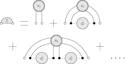
Refer to caption
Figure 16: Pictorial representation of the second Dyson-Schwinger equation (133). Each one-line-irreducible diagram may be constructed by aligning some diagrams next to each other and straddling them with a connected diagram.

This graphical equation is equivalent to

Σ^ab=(κ^1)ab+cd(κ^2)ac,dbG^cd+cefd(κ^3)ac,ef,dbG^ceG^fd+.subscript^Σ𝑎𝑏subscriptsubscript^𝜅1𝑎𝑏subscript𝑐𝑑subscriptsubscript^𝜅2𝑎𝑐𝑑𝑏subscript^𝐺𝑐𝑑subscript𝑐𝑒𝑓𝑑subscriptsubscript^𝜅3𝑎𝑐𝑒𝑓𝑑𝑏subscript^𝐺𝑐𝑒subscript^𝐺𝑓𝑑\widehat{\Sigma}_{ab}=(\widehat{\kappa}_{1})_{ab}+\sum_{cd}(\widehat{\kappa}_{2})_{ac,db}\widehat{G}_{cd}+\sum_{cefd}(\widehat{\kappa}_{3})_{ac,ef,db}\widehat{G}_{ce}\widehat{G}_{fd}+\ldots\ . (133)

This is the second Dyson-Schwinger equation. The two Dyson-Schwinger equations simplify for Z^=z𝟙^𝑍𝑧double-struck-𝟙\widehat{Z}=z\mathbb{1} (Z^ab=zδabsubscript^𝑍𝑎𝑏𝑧subscript𝛿𝑎𝑏\widehat{Z}_{ab}=z\delta_{ab}) since in this case G^=G(z)𝟙^𝐺𝐺𝑧double-struck-𝟙\widehat{G}=G(z)\mathbb{1} and Σ^=Σ(z)𝟙^ΣΣ𝑧double-struck-𝟙\widehat{\Sigma}=\Sigma(z)\mathbb{1}, where G(z)𝐺𝑧G(z) and Σ(z)Σ𝑧\Sigma(z) are complex scalar functions. In effect, equations (132) and (133) reduce after taking the normalized trace to scalar equations

G(z)=(zΣ(z))1𝐺𝑧superscript𝑧Σ𝑧1G(z)=\left(z-\Sigma(z)\right)^{-1} (134)

and

Σ(z)=κ1+κ2G(z)+κ3G2(z)+Σ𝑧subscript𝜅1subscript𝜅2𝐺𝑧subscript𝜅3superscript𝐺2𝑧\Sigma(z)=\kappa_{1}+\kappa_{2}G(z)+\kappa_{3}G^{2}(z)+\ldots (135)

where

κn=limN1NTrHn.subscript𝜅𝑛subscript𝑁1𝑁delimited-⟨⟩delimited-⟨⟩Trsuperscript𝐻𝑛\kappa_{n}=\lim_{N\rightarrow\infty}\frac{1}{N}\langle\langle\mathrm{Tr}H^{n}\rangle\rangle\ . (136)

These coefficients are connected planar (or free) cumulants as they are defined as sums over all connected planar diagrams with n𝑛n external legs. The generating function for planar cumulants is called R transform in free probability and it is defined as

R(z)=κ1+κ2z+κ3z2+=n=1κnzn1.𝑅𝑧subscript𝜅1subscript𝜅2𝑧subscript𝜅3superscript𝑧2superscriptsubscript𝑛1subscript𝜅𝑛superscript𝑧𝑛1R(z)=\kappa_{1}+\kappa_{2}z+\kappa_{3}z^{2}+\ldots=\sum_{n=1}^{\infty}\kappa_{n}z^{n-1}\ . (137)

Using the R transform one can concisely write the second Dyson-Schwinger equation (135)

Σ(z)=R(G(z)).Σ𝑧𝑅𝐺𝑧\Sigma(z)=R(G(z)). (138)

Inserting this into the first Dyson-Schwinger equation (134) one eventually obtains the formula

G(z)=1zR(G(z)),𝐺𝑧1𝑧𝑅𝐺𝑧G(z)=\frac{1}{z-R(G(z))}, (139)

which was earlier mentioned in the main text (15).

Generalization of these equations to non-hermitian matrices is straightforward. The Dyson-Schwinger equations (132) and (133) have the same form as for hermitian matrices but a slighly more complex index structure, since the N×N𝑁𝑁N\times N hermitian matrices are considered as quaternionic matrices (or equivalently 2N×2N2𝑁2𝑁2N\times 2N matrices with a particular block structure) (17) and (18). The additional index structure takes care of parts of quaternion (positions of blocks in the 2N×2N2𝑁2𝑁2N\times 2N matrices). After taking the block-trace (110)one gets a matrix equation for 2×2222\times 2 matrices (quaternions) (28) instead of scalar equation (139).

References

  • (1) M. L. Mehta, Random matrices (Elsevier, Amsterdam, 2004).
  • (2) A. Crisanti, G. Paladin, A. Vulpiani, Products of random matrices , Random matrices and their applications, (Springer-Verlag, Berlin Heidelberg, 1993).
  • (3) J. E. Cohen, H. Kesten and C.M. Newman (eds), Random matrices and their applications, Contemporary Mathematics 50, (Providence, RI: American Mathematical Society, 1986).
  • (4) T. Guhr, A. Müller-Groeling, H. A. Weidenmüller, Phys. Rep. 299, 189 (1998).
  • (5) G. Akemann, J. Baik, P. Di Francesco (Ed.), The Oxford Handbook of Random Matrix Theory, (Oxford University Press, Oxford, 2011).
  • (6) A. M. Tulino and S. Verdú, Random Matrix Theory and Wireless Communications, Foundations and Trends in Communications and Information Theory, 1 1 (2004).
  • (7) G. W. Anderson, A. Guionnet, O. Zeitouni, An Introduction to Random Matrices, (Cambridge University Press, Cambridge, 2009).
  • (8) D. V. Voiculescu, J. Funct. Anal. 66, 323 (1986).
  • (9) D. V. Voiculescu, J. Operator Theory, 18, 223 (1987).
  • (10) D. V. Voiculescu, K. J. Dykema, A. Nica, Free random variables, CRM Monograph Series, Vol. 1 (American Mathematical Society, Providence, RI, 1992).
  • (11) R. Speicher, Math. Ann. 298, 611 (1994).
  • (12) N. R. Rao and R. Speicher, Elect. Comm. in Probab. 12, 248 (2007).
  • (13) Z. Burda, R.A. Janik and B. Waclaw, Phys. Rev. E 81 041132 (2010).
  • (14) G. Akemann and Z. Burda, J. Phys. A: Math. Theor. 45, 465201 (2012).
  • (15) F. Haake, F. Izrailev, N. Lehmann et al., Z.Phys. B88 359 (1992).
  • (16) Y. V. Fyodorov, H.-J.Sommers, JETP Letters 63, 1026 (1996).
  • (17) Y. V. Fyodorov, H.-J.Sommers, J. Math. Phys. 38, 1918 (1997).
  • (18) Y. V. Fyodorov, D. V. Savin, H.-J. Sommers, Phys. Rev. E55, R4857 (1997).
  • (19) R. Janik, M. Nowak, I. Zahed, Phys.Lett. B392 155 (1997).
  • (20) J. J. M. Verbaarschot, Nucl.Phys. A642 305 (1998).
  • (21) C. Biely, S. Thurner, Quant. Finance 8, 705 (2008).
  • (22) A. Jarosz, Hermitian and non-Hermitian covariance estimators for multivariate Gaussian and non-Gaussian assets from random matrix theory, arXiv:1010.5220.
  • (23) H.-J. Sommers, A. Crisanti, H. Sompolinsky, and Y. Stein, Phys. Rev. Lett. 60, 1895 (1988).
  • (24) S. Drozdz, J. Kwapien, A. A. Ioannides, Acta Phys. Pol. B42 987 (2011).
  • (25) E. Gudowska-Nowak, R. A. Janik, J. Jurkiewicz and M. A. Nowak, Nucl Phys. B670 479 (2003).
  • (26) Z. Burda, J. Grela, M. A. Nowak, W. Tarnowski, P. Warchol, Phys.Rev.Lett. 113 104102 (2014).
  • (27) K. Rajan, L.F. Abbott Phys Rev Lett. 97, 188104 (2006).
  • (28) S.E. Skipetrov, A. Goetschy, J. Phys. A: Math. Theor. 44, 065102 (2011).
  • (29) R. A. Janik, Ph.D. Thesis, Jagiellonian University, Cracow 1996, (unpublished).
  • (30) R. A. Janik, M. A. Nowak, G. Papp and I. Zahed, Nucl.Phys. B 501, 603 (1997).
  • (31) R. A. Janik, M. A. Nowak, G. Papp and I. Zahed, Acta Phys. Polon. B28 2949 (1997).
  • (32) R. A. Janik, M. A. Nowak, G. Papp, J. Wambach and I. Zahed, Phys. Rev. E55 4100 (1997).
  • (33) J. Feinberg and A. Zee, Nucl. Phys. B501 643 (1997).
  • (34) J. Feinberg and A. Zee, Nucl. Phys. B504 579 (1997).
  • (35) A. Jarosz and M. A. Nowak, A Novel Approach to Non-Hermitian Random Matrix Models, arXiv:math-ph/0402057.
  • (36) A. Jarosz and M.A. Nowak, J. Phys. A39 10107 (2006).
  • (37) Z. Burda, R. A. Janik, M. A. Nowak, Phys. Rev. E 84, 061125 (2011).
  • (38) T. Rodgers, J. Math. Phys. 51 093304 (2010).
  • (39) Ch. Bordenave, P. Caputo, D. Chafai, Commun. Pure Appl. Math. 67 621 (2014).
  • (40) A. Jarosz, Summing free unitary random matrices, arXiv:1010.5220.
  • (41) J. T. Chalker and B. Mehlig, Phys. Rev. Lett. 81 3367 (1998).
  • (42) R.A. Janik, W. Norenberg, M.A. Nowak, G. Papp and I. Zahed, Phys. Rev. E60 2699 (1999).
  • (43) G. ’t Hooft, Nucl. Phys. B 72, 461 (1974).
  • (44) E. Brezin, C. Itzykson, G. Parisi and J.-B. Zuber, Commun. Math. Phys. 59, 35 (1978).
  • (45) D. Bessis, C. Itzykson and J.-B. Zuber, Adv. Appl. Math. 1, 109 (1980).
  • (46) V. L. Girko, Spectral theory of random matrices, in Russian (Nauka, Moscow, 1988).
  • (47) J. Ginibre, J. Math. Phys. 6 440–449 (1965).
  • (48) Y. V. Fyodorov, B. A. Khoruzhenko, H.-J. Sommers, Phys.Lett. A226 46 (1997).
  • (49) U. Haagerup, H. Schultz, S. Thorbjørnsen, Adv. Math. 204 1 (2006).
  • (50) G. W. Anderson, Ann. Probab. 41 2103 (2013)
  • (51) S. Belinschi, T. Mai and R. Speicher, Analytic subordination theory of operator-valued free additive convolution and the solution of a general random matrix problem, arXiv:1303.3196.
  • (52) C. M. Newman, Commun. Math. Phys. 103 121–126 (1986).
  • (53) P. J. Forrester, Asymptotics of finite system Lyapunov exponents for some random matrix ensembles, arXiv:1501.05702.
  • (54) G. Akemann, Z. Burda, M. Kieburg, J. Phys. A: Math. Theor. 47 395202 (2014).
  • (55) R. R. Mueller, IEEE Trans. Inf. Theor. 48 2086 (2002).
  • (56) G. Akemann, M. Kieburg, L. Wei, J. Phys. A: Math. Theor. 46, 275205 (2013).
  • (57) J.-P. Bouchaud, L. Laloux, M.A. Miceli, M. Potters, European Physical Journal B 2 201-207 (2007).
  • (58) G. Livan, L. Rebecchi, Eur. Phys. J. B 85, 213 (2012).