The Fractional Quantum Hall States at $\nu=13/5$ and $12/5$ and their Non-Abelian Nature

Abstract

Topological quantum states with non-Abelian Fibonacci anyonic excitations are widely sought after for the exotic fundamental physics they would exhibit, and for universal quantum computing applications. The fractional quantum Hall (FQH) state at filling factor $\nu=12/5$ is a promising candidate, however, its precise nature is still under debate and no consensus has been achieved so far. Here, we investigate the nature of the FQH $\nu=13/5$ state and its particle-hole conjugate state at $12/5$ with the Coulomb interaction, and address the issue of possible competing states. Based on a large-scale density-matrix renormalization group (DMRG) calculation in spherical geometry, we present evidence that the essential physics of the Coulomb ground state (GS) at $\nu=13/5$ and $12/5$ is captured by the $k=3$ parafermion Read-Rezayi state ($\text{RR}_{3}$), including a robust excitation gap and the topological fingerprint from entanglement spectrum and topological entanglement entropy. Furthermore, by considering the infinite-cylinder geometry (topologically equivalent to torus geometry), we expose the non-Abelian GS sector corresponding to a Fibonacci anyonic quasiparticle, which serves as a signature of the $\text{RR}_{3}$ state at $13/5$ and $12/5$ filling numbers.

Introduction.— While fundamental particles in nature are either bosons or fermions, the emergent excitations in two-dimensional strongly-correlated systems may obey fractional or anyonic statistics Tsui1982 ; Laughlin1983 . After two decades of study Willett1987 ; Pan1999 ; Xia2004 ; Choi2008 ; Pan2008 ; Kumar2010 ; Radu2008 ; Dolev2012 ; Willett2013 ; Baer2014 ; Chi2012 , current interest in exotic excitations focuses on states of matter with non-Abelian quasiparticle excitations Moore ; Greiter ; Read1999 , and their potential applications to the rapidly evolving field of quantum computation and cryptography Nayak ; Kitaev2003 ; Freedman2002 ; Sarma2005 ; Hormozi2007 ; Bonesteel2005 . So far the most promising platform for realization of non-Abelian statistics is the fractional quantum Hall (FQH) effect in the first excited Landau level, and two of the most interesting examples are at filling factors $\nu=5/2$ and $12/5$. The $\nu=5/2$ state is widely considered to be the candidate for the Moore-Read state hosting non-Abelian Majorana quasiparticles Moore ; Greiter ; Read1999 . Experiments have revealed that the $12/5$ state appears to behave differently from the conventional FQH effect Xia2004 ; Kumar2010 , and may also be a candidate state for hosting non-Abelian excitations. However, the exact nature of the FQH $12/5$ state is still undetermined due to the existence of other possible competing candidate states.

Several ground-state (GS) wavefunctions have been proposed Read1999 ; Rezayi2009 ; Bonderson2008 ; Bonderson2012 ; Sreejith2011 ; Sreejith2013 as models for the observed FQH effect at $\nu=12/5$ Xia2004 ; Kumar2010 ; Chi2012 . The most exciting candidate is the $k=3$ parafermion state proposed by Read and Rezayi ($\text{RR}_{3}$)Read1999 . This $\text{RR}_{3}$ state describes a condensate of three-electron clusters that forms an incompressible state at $\nu=13/5$ Read1999 . One can also construct the particle-hole partner of the RR₃ state to describe the $12/5$ FQH effect. Besides the $\text{RR}_{3}$ state, some competing candidates for $\nu=13/5$ or $12/5$ exist: a hierarchy state Haldane1983 ; Halperin1984 , a Jain composite-fermion (CF) state JainBook , a generalization of the non-Abelian Pfaffian state by Bonderson and Slingerland (BS) Bonderson2008 ; Bonderson2012 , and a bipartite CF state Sreejith2011 ; Sreejith2013 . So far, the true nature of the $12/5$ and $13/5$ FQH states remains undetermined. The main challenges in settling this issue are the limited computational ability and the lack of an efficient diagnostic method. For example, from exact diagonalization (ED) calculations in the limited feasible range of system sizes, it is found that the overlaps between the Coulomb GS at $\nu=12/5$ and different model wavefunctions are all relatively large Read1999 ; Bonderson2012 , while the extrapolated GS energies of the RR₃ and BS states are very close in the thermodynamic limit Wojs2009 ; Bonderson2012 . Taken as a whole, previous studies have left the nature of the Coulomb GS at $\nu=13/5$ and $12/5$ unsettled.

Recently, there has been growing interest in connecting quantum entanglement Kitaev2006 ; Levin2006 ; Haldane2008 ; YZhang2012 with emergent topological order Wen1990 ; Wen1995 in strongly interacting systems, which offers a new route to identification of the precise topological order of a many-body state. Although characterization of entanglement has been successfully used to identify various well-known types of topological order Haque2007 ; Lauchli2010 ; Papic2011 ; Cincio2013 ; Zatel2013 ; Tu2013 ; HCJiang ; WZhu2014 , application of the method to a system with competing phases still faces challenges when ED studies suffer from strong finite size effects, and other methods such as quantum Monte-Carlo suffer from sign problems. The recent development of the high efficiency density-matrix renormalization group (DMRG) in momentum space JizeZhao2011 ; Zatel2013 allows the study of such systems in sphere and cylinder geometries, both of which can be used to make concrete predictions of the physics of real systems in the thermodynamic limit. Here we combine these advances, and use these two geometries to address the long-standing issues of the FQH at $\nu=12/5$ and $13/5$.

In this paper, we study the FQH at $\nu=12/5$ and $13/5$ filling by using the state-of-the-art density-matrix renormalization group (DMRG) numerical simulations. By studying large systems up to $N_{e}=36$ on spherical geometry, we establish that the Coulomb GS at $\nu=13/5$ is an incompressible FQH state, protected by a robust neutral excitation gap $\Delta_{n}\approx 0.012(e^{2}/l_{B})$. Crucially, we show that the entanglement spectrum (ES) fits the corresponding $SU(2)_{3}$ conformal field theory (CFT) which describes the edge structure of the parafermion $\text{RR}_{3}$ state. The topological entanglement entropy (TEE) is also consistent with the predicted value for the $\text{RR}_{3}$ state, indicating the emergence of Fibonacci anyonic quasiparticles. Moreover, we also perform a finite-size scaling analysis of the GS energies for $\nu=12/5$ states at different shifts corresponding to the particle-hole-conjugate of the $\text{RR}_{3}$ state, the Jain state and BS state. Finite-size scaling confirms that the ground state with topological shift $\mathcal{S}=-2(3)$ (where RR₃ state is expected to occur) is energetically favored in the thermodynamic limit. Finally, to explicitly demonstrate the topological degeneracy, we obtain two topological distinct GS sectors on the infinite cylinder using infinite-size DMRG. While one sector is the identity sector matching to the GS from the sphere, the new sector is identified as the non-Abelian sector with a Fibonacci anyonic quasiparticle through its characteristic ES and TEE. Thus we establish that the essence of the FQH state at $\nu=13/5$ is fully captured by the non-Abelian parafermion $\text{RR}_{3}$ state (and by its particle-hole conjugate at $\nu$ = 12/5) and show that it is stable against perturbations as we change the Haldane pseudopotentials and the layer width of the system.

Model and Method.— We use the Haldane representation Haldane1983 ; Fano1986 ; Greiter2011 in which the $N_{e}$ electrons are confined on the surface of a sphere surrounding a magnetic monopole of strength $Q$. In this case, the orbitals of the $n$-th LL are represented as orbitals with azimuthal angular momentum $-L,-L+1,...,L$, with $L=Q+n$ being the total angular momentum. The total magnetic flux through the spherical surface is quantized to be an integer $N_{s}=2L$. Assuming that electron spins are fully-polarized and neglecting Landau-level mixing, the Hamiltonian in the spherical geometry can be written as:

$$H=\frac{1}{2}\sum_{m_{1}+m_{2}=m_{3}+m_{4}}\langle m_{1},m_{2}|V|m_{3},m_{4}\rangle\hat{a}^{\dagger}_{m_{1}}\hat{a}^{\dagger}_{m_{2}}\hat{a}_{m_{3}}\hat{a}_{m_{4}}$$

where $\hat{a}^{\dagger}_{m}$ ($\hat{a}_{m}$ ) is the creation (annihilation) operator at the orbital $m$ and $V$ is the Coulomb interaction between electrons in units of $e^{2}/l_{B}$ with $l_{B}$ being the magnetic length. The two-body Coulomb interaction element can be decomposed as

$$\langle i,j|V|p,q\rangle=\sum_{l=0}^{2L}\sum_{m=-l}^{l}\langle L,i;L,j|l,m\rangle\langle l,m|L,p;L,q\rangle\mathcal{V}^{n}(l)$$

where $\langle L,i;L,j|l,m\rangle$ is the Clebsch-Gordan coefficients and $\mathcal{V}^{n}(l)$ is the Haldane pseudopotential representing the pair energy of two electrons with relative angular momentum $2L-l$ in $n$-th LL Haldane1983 ; supple . For electrons at fractional filling factor $\nu$, $N_{s}=\nu^{-1}N_{e}-\mathcal{S}$, where $\mathcal{S}$ is the curvature-induced “shift” on the sphere.

Our calculation is based on the unbiased DMRG method White ; Xiang1996 ; Shibata ; Feiguin2008 ; JizeZhao2011 ; Hu2012 , combined with ED. The (angular) momentum-space DMRG allows us to use the total electron number $N_{e}$ and the total z-component of angular momentum $L^{tot}_{z}=\sum_{i=1}^{N_{e}}m_{i}$ as good quantum numbers to reduce the Hilbert subspace dimension JizeZhao2011 . Here, we report the result at $\nu=13/5(12/5)$ with electron number up to $N_{e}=36(22)$ by keeping up to $30000$ states with optimized DMRG, which allows us to obtain accurate results for energy and the ES on much larger system sizes beyond the ED limit ($N^{ED}_{e}=24(16)$ at $\nu=13/5(12/5)$).

Groundstate Energy, Energy Spectrum and Neutral Gap.— We first compute the GS energies for a number of systems up to $N_{e}=36$ at $\nu=13/5$, with a shift $\mathcal{S}=3$ consistent with the $\text{RR}_{3}$ state. As shown in the low-lying energy spectrum in the inset of Fig. 1(b) obtained from ED for $N_{e}=21$, the GS is located in the $L^{tot}=0$ sector and is separated from the higher energy continuum by a finite gap, which signals an incompressible FQH state. The extrapolation of the GS energy to the thermodynamic limit can be carried out using a quadratic function of $1/N_{e}$ (blue line), or a linear fit in $1/N_{e}$ (red line) after renormalizing the energy by $\sqrt{2Q\nu/N_{e}}$ to take into account the curvature of the sphere Morf1985 , as shown in Fig. 1(a). We obtain the $E_{0}/N_{e}=-0.38458(24)$ (blue line) and $-0.38487(9)$ (red line), which demonstrates consistency between the two extrapolating schemes.

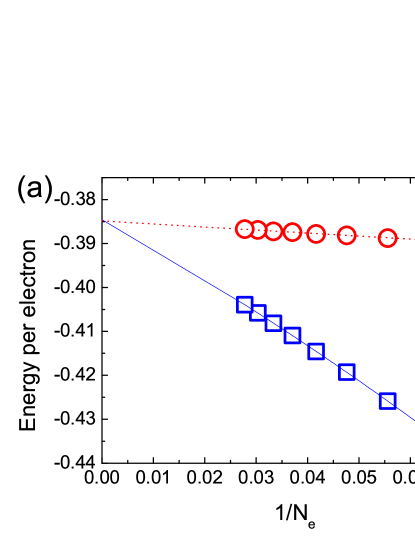
Figure 1: (a) The groundstate energy per electron (blue dots) corresponding to the $\nu=13/5$ state. The blue line shows the extrapolated values obtained using a quadratic function of $1/N_{e}$. The red dots shows the rescaling energy by a renormalized magnetic length and the red line is the linear fitting. (b) The neutral gap $\Delta_{n}$ for $13/5$ state as a function of the $1/N_{e}$ ($b$ is the layer-width parameter supple ). Inset: Energy spectrum versus total angular momentum $L^{tot}$ for $N_{e}=21$. $\Delta_{n}$ is defined as the energy difference between the lowest energy state (in $L^{tot}=0$) and the first excited state (in $L^{tot}\neq 0$).

We also calculated the neutral excitation gap $\Delta_{n}$ at $\nu=13/5$ note1 . This is equivalent to the energy difference between the GS and the “roton minimum”Haldane1985 ; GMP ; BoYang2012 as illustrated in the inset of Fig. 1(b). The roton minimum corresponds to the lowest excitation energy of a quasielectron-quasihole pair BoYang2012 . Fig. 1(b) shows $\Delta_{n}$ as a function of $1/N_{e}$, where the large-system results indicate that the neutral gap approaches a nonzero value $\Delta_{n}\approx 0.012\pm 0.001$ for $N_{e}\geq 21$. Since the hamiltonian in this paper is particle-hole symmetric, the neutral gap at $\nu=12/5$ and $13/5$ are expected to be identical note2 . In addition, if the effect of finite layer-width is consideredsupple , the neutral-excitation gap is reduced but still remains consistent with a nonzero value (Fig. 1(b)).

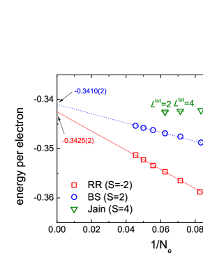
Figure 2: Finite-size extrapolation of the ground-state (GS) energies for different shifts corresponding to different candidate states at $\nu=12/5$. All energies have been rescaled by the renormalized magnetic length. The angular momentum of the GS is shown whenever it is nonzero ($L^{tot}\neq 0$).

Competing states.— In Fig. 2, we compare the GS energies per electron of three known candidates for $\nu=12/5$: the particle-hole conjugate of the $\text{RR}_{3}$ state with a shift $\mathcal{S}=-2$, the non-Abelian BS state with $\mathcal{S}=2$ Bonderson2008 , and Jain state with $\mathcal{S}=4$. We find that the lowest-energy state for the Jain state shift ($\mathcal{S}=4$) in larger system sizes has a total angular momentum $L^{tot}\neq 0$, indicating that it represents excitations of some other incompressible state rather than the Coulomb GS at $\nu=12/5$ Sreejith2013 . Secondly, the GSs with the $\text{RR}_{3}$ and BS shifts continue to have $L^{tot}=0$ for the systems that we have studied, and the extrapolation based on the result for $10\leq N_{e}\leq 22$ leads to $E_{0}/N_{e}=-0.3425$ for the $\text{RR}_{3}$ state and $E_{0}/N_{e}=-0.3410$ for the BS state, respectively. Compared to the previous studies Bonderson2012 ; Wojs2009 , the extrapolation errors are reduced by the inclusion of larger system sizes obtained using DMRG. Our calculations suggest that the $\text{RR}_{3}$ state with shift $\mathcal{S}=-2$($\mathcal{S}=3$) is energetically favored as the GS at $\nu=12/5(13/5)$. Our results are consistent with the interpretation that the $\text{RR}_{3}$ state describes the true GS (see the full evidence below), while the other states at nearby shifts correspond to states with quasiparticle or quasihole excitations.

Orbital ES.— Li and Haldane first established that the orbital ES of the GS of FQH phase contains information about the counting of their edge modes Haldane2008 ; Wen1995 . Thus, the orbital ES provides a “fingerprint” of the topological order, which can be used to identify the emergent topological phase in a microscopic Hamiltonian Haldane2008 ; Lauchli2010 ; Papic2011 ; Cincio2013 ; Zatel2013 .

As a model FQH state, the $\text{RR}_{3}$ parafermion state can be represented by its highest-density root configuration pattern of “1110011100… 11100111”, corresponding to a generalized Pauli principle of “no more than three electrons in five consecutive orbitals” Bergholtz2005 ; Bernevig2008a ; Bernevig2008b . Consequently, the orbital ES depends on the number of electrons in the partitioned subsystem supple . In Fig. 3, we show the orbital ES of three distinct partitions for system size $N_{e}=36$ for Coulomb GS. For $3n$ electrons in subsystem (Fig. 3(a)), the leading ES displays the multiplicity-pattern $1,1,3,6,12$ in the first five angular momentum sectors $\Delta L^{A}_{z}=0,1,2,3,4$. For $3n+1$ or $3n+2$ electrons in subsystem (Fig. 3(b-c)), the ES shows the multiplicity-pattern of $1,2,5,9$ in the $\Delta L=0,1,2,3$ momentum sectors. The above characteristic multiplicity-patterns of the low-lying ES agree with the predicted edge excitation spectrum of the $\text{RR}_{3}$ state obtained either from its associated CFT, or the “$\leq 3$ in 5” exclusion statistics rule supple ; note3 .

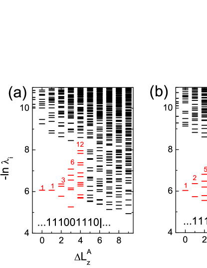
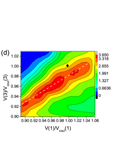
Figure 3: (a-c) The low-lying orbital ES of $N_{e}=36$ are shown for three different partitions. The lower ES level counting in the sector $\Delta L^{A}_{z}=0,1,2,3,4$ are labeled by color, where $\Delta L^{A}_{z}=L^{A}_{z}-L^{A}_{z,min}$ with $L^{A}_{z,min}$ as the quantum number where the primary field occurs. The entanglement gap of orbital ES of $N_{e}=24$ is shown for partition (d) with $3n$ electrons and (e) with $3n+1$ electrons in the subsystem as a function of pseudopotential $\mathcal{V}^{1}(1)/\mathcal{V}^{1}_{Coul}(1)$ and $\mathcal{V}^{1}(3)/\mathcal{V}^{1}_{Coul}(3)$, where $\mathcal{V}^{1}_{Coul}(l)$ are the Coulomb values of pseudopotentials. The black point corresponds to the Coulomb point.

In addition, we vary the Haldane pseudopotentials $\mathcal{V}^{1}(1)$ and $\mathcal{V}^{1}(3)$ (keeping all others at their Coulomb-interaction values), and map out an ES-gap diagram which illustrates the robustness of the FQH state as the interaction parameters are changedMorf2010 ; Peterson2008 ; Biddle2011 ; Pakrouski2014 . In Fig. 3, we plot the entanglement gap (for the lowest-$L^{z}$ ES level)Haldane2008 ; JizeZhao2011 as a function of $\mathcal{V}^{1}(1)/\mathcal{}\mathcal{V}^{1}_{Coul}(1)$ and $\mathcal{V}^{1}(3)/\mathcal{V}^{1}_{Coul}(3)$, where $\mathcal{V}^{1}_{Coul}(l)$ are the Coulomb values of pseudopotentials. We find that the entanglement gap is robust in a region centered at an approximately-fixed $\mathcal{V}^{1}(1)/\mathcal{V}^{1}(3)$ ratio (indicated by the white line). Away from that, for the regime $\mathcal{V}^{1}(1)/\mathcal{V}^{1}_{Coul}(1)<0.92$ and $\mathcal{V}^{1}(3)/\mathcal{V}^{1}_{Coul}(3)>0.98$, we find a rapid drop of the entanglement gap indicating a quantum phase transition. We have also studied the effect of the ES of modifying the Coulomb interaction with a realistic layer width (b) supple , and find that the $\text{RR}_{3}$ state persists until $\textit{b}/l_{B}\sim 2$, which is qualitatively consistent with the results of varying $\mathcal{V}^{1}(1)$ and $\mathcal{V}^{1}(3)$.

Topological Entanglement Entropy.— For a two-dimensional gapped topologically-ordered state, the dependence of the entanglement entropy $S_{A}(l_{A})$ of the subsystem A on the finite boundary-cut length $l_{A}$ has the form $S_{A}(l_{A})=\alpha l_{A}-\gamma$, where TEE $\gamma$ is related to the total quantum dimension $\mathcal{D}$ by $\gamma=\ln\mathcal{D}$ Kitaev2006 ; Levin2006 . We have extracted the TEE using our largest system, $N_{e}=36$ supple . The TEE obtained was $\gamma=1.491\pm 0.091$, consistent with the theoretically-predicted value $\gamma=\ln\mathcal{D}=\ln\sqrt{5(1+\phi^{2})}\approx 1.447$ for the $\text{RR}_{3}$ state, where each non-Abelian Fibonacci anyon quasiparticle contributes an individual quantum dimension $d_{F}=\phi=(\sqrt{5}+1)/2$ ($\phi$ denotes the Golden Ratio). The appearance of $d_{F}=\phi$ is a signal of the emergence of Fibonacci anyon quasiparticles, and arises because two Fibonacci quasiparticles may fuse either into the identity or into a single Fibonacci quasiparticle WZhu2014 . This exotic property makes Fibonacci quasiparticles capable of universal quantum computation Nayak .

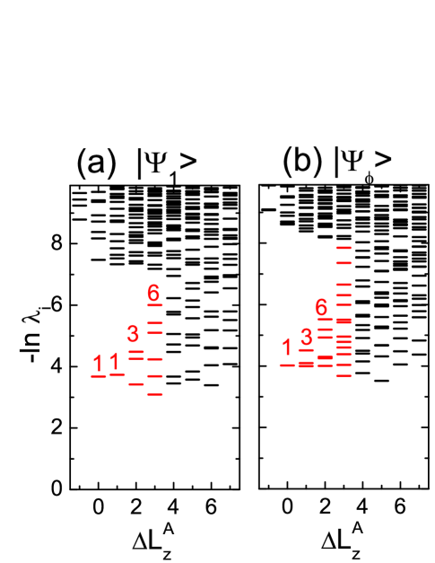
Figure 4: (a-b) The low-lying orbital ES of $\Psi_{1}$ and $|\Psi_{\phi}\rangle$ by setting $L_{y}=24l_{B}$. $|\Psi_{1(\phi)}\rangle$ denotes the GS with identity $\openone$ (Fibonacci $\phi$) anyonic quasiparticle. (c) Energy difference and (d) entropy difference between $|\Psi_{1}\rangle$ and $|\Psi_{\phi}\rangle$, obtained from infinite DMRG on cylinder geometry with varying $L_{y}$. The error bars are determined based on results from ten different infinite DMRG calculations for each sectorsupple .

Topological Degeneracy on the infinite cylinder.— Topologically-ordered states have characteristic GS degeneracies on compactified spaces. To access the different topological sectors at $\nu=13/5$, we implemented the infinite-size DMRG in cylinder geometry with a finite circumference $L_{y}$ Zatel2013 ; Zatel2015 ; supple . For each value of $L_{y}$, we repeatedly calculated GSs using different random initializations for the infinite DMRG optimization. We found that each infinite DMRG simulation converged to one of the two states: $|\Psi_{1}\rangle$ and $|\Psi_{\phi}\rangle$. These states are distinguishable by their orbital ES as shown in Fig. 4: $|\Psi_{1}\rangle$ has the same ES structure as in Fig. 3(a-c), which matches the identity sector with root configuration “$\ldots 0111001110\ldots$”. On the other hand, $|\Psi_{\phi}\rangle$ shows the ES multiplicity pattern $1,3,6,13,...$, which identifies the spectrum as that of the Fibonacci non-Abelian sector with root configuration “$\ldots 1010110101\ldots$” supple . Furthermore, these two groundstates are indeed energetically degenerate, with an energy-difference per electron of less than $0.0002$ with $L_{y}=24l_{B}$, while the entropy difference between these two states is around $\Delta S\approx\ln\phi\approx 0.48$, consistent with the quantum dimension of the Fibonacci quasiparticle. Combining this with the fivefold center-of-mass degeneracy, we have obtained all the 10 predicted degenerate $\text{RR}_{3}$ GSs on infinite cylinder (or torus).

Summary and discussion.— We have presented what we believe to be compelling evidence that the essence of the Coulomb-interaction ground states at $\nu=13/5$ and $12/5$ is indeed captured by the parafermion $k=3$ Read-Rezayi state $\text{RR}_{3}$, in which quasiparticles obey non-Abelian “Fibonacci-anyon” statistics. The neutral excitation gap is found to be a finite value $\Delta_{n}\approx 0.012e^{2}/l_{B}$ in the thermodynamic limit. Results for the entanglement spectrum “fingerprint” and the value of the topological entanglement entropy show that the edge structure and bulk quasiparticle statistics are consistent with the prediction bases on the $\text{RR}_{3}$ state. Additionally, we find two topologically-degenerate groundstate sectors on the infinite cylinder, respectively corresponding to the identity and the Fibonacci anyonic quasiparticle, which fully confirms the $\text{RR}_{3}$ state, without input of any features (such as shift) taken from the model wavefunction, that might have biased the calculation. The current work opens up a number of directions deserving further exploration. For example, while the FQH $\nu=12/5$ state has been observed in experiment, there is no evidence of a FQH phase at $\nu=13/5$ in the same systems Xia2004 ; Kumar2010 . So far it is not clear whether this absence is due to a broken particle-hole symmetry from Landau level mixing, or other asymmetry effects such as differences in the quantum wells Pan2008 . Our numerical studies suggest that the outlook for the existence of such a state at $13/5$ is promising, and some positive signs of this may have already been observed very recently ZnO2015 . Numerical studies may also further suggest how various other exotic FQH states in the second Landau level at different filling-factors may be stabilized.

Note added.— After the completion of this work, we became aware of overlapping results in Refs. Mong2015 .

WZ thanks Z. Liu for fruitful discussion, N. Regnault and A. Wójs for useful comments. We also thank X. G. Wen for stimulating discussion and M. Zaletel, R. S. K. Mong, F. Pollamann for private communication prior to publication. This work is supported by the U.S. Department of Energy, Office of Basic Energy Sciences under grants No. DE-FG02-06ER46305 (WZ, DNS) and DE-SC0002140 (FDMH), and the National Science Foundation through the grant DMR-1408560 (SSG). FDMH also acknowledges support from the W. M. Keck Foundation. WZ also acknowledges the support from MRSEC DMR-1420541 and PREM DMR-1205734 for a visit to Princeton where this work was completed.

In this supplemental material, we provide more details of the calculation and results which were not given in the main text. In Sec. I, we briefly summarize the Haldane pseudopotentials in disk and spherical geometries used for calculation in the main text. In Sec. II, we give a detailed analysis of edge excitations of the fermionic Read-Rezayi (RR) $k=3$ state, based on the root configurations. In Sec. III, we introduce the effect of finite layer-width and show the evolution of entanglement spectrum (ES) with the change of the layer width. In Sec. IV, we extract the topological entanglement entropy (TEE) based on the dependence of entropy on the length of the orbital cut. In Sec. V, we show the ES of the $\nu=12/5$ state, which is a particle-hole-conjugate state of the $\nu=13/5$ state. In Sec. VI, we introduce the numerical details of the infinite-size density-matrix renormalization group (DMRG) algorithm on cylinder geometry.

Appendix A I. Pseudopotentials

HaldaneHaldane1983 first pointed out that, any rotationally-invariant two-body interaction can be completely described by a set of “pseudopotential” $\mathcal{V}(m)$ with $m\geq 0$, if projected onto a single Landau level. The pseudopotential describes the energy of a pair of particles in a state of given relative angular momentum $m$. This formalism turned out to be useful not just for describing the details of the interaction, but also for understanding the microscopic conditions of the fractional quantum Hall (FQH) states in such systems. Here we focus on the pseudopotential formalism for two-body Coulomb interaction, in two specific geometries, the disk (or plane) and the sphere, respectively.

A.1 1. Disk (plain) geometry

In disk geometry, the Haldane pseudopotentials have been obtained many places Haldane1983 :

$$\mathcal{V}^{(n)}_{m}=<n,m|V(r)|n,m>=\int\limits_{0}^{\infty}dqq[L_{n}(\frac{q^{2}}{2})]^{2}L_{m}(q^{2})e^{-q^{2}}V(q)$$ (1)

Here $|n,m\rangle$ is a two electron state with relative (azimuthal) angular momentum $m$ in the $n$-th Landau level. $L_{m}(x)$ is a Laguerre polynomial, and the two-body interaction $V(r)=\int d\textbf{q}V(q)e^{i\textbf{q}\cdot\textbf{r}}$.

For the ideal Coulomb interaction in two dimensions $V(r)=1/r$ ( in unit of $\frac{e^{2}}{\varepsilon l_{0}}$), we have, for the first Landau level,

$$\mathcal{V}^{(n=0)}(m)=\frac{\Gamma(m+1/2)}{2m!}$$

and for the second Landau level:

$$\mathcal{V}^{(n=1)}(m)=\frac{\Gamma(m+1/2)}{2m!}\frac{(m-3/8)(m-11/8)}{(m-1/2)(m-3/2)}$$

A.2 2. Sphere geometry

In spherical geometry, we first define the total angular momentum $L=Q+n$, where $Q$ is the strength of the magnetic monopole in the center of the sphere and $n$ is Landau level index. The pseudopotential $\mathcal{V}^{n}(l)$ is defined as the interaction energy of a pair of electrons as a function of their pair angular momentum $l$. In this expression, the pseudopotential for particles in a single Landau level is evaluated from the matrix element

$$\mathcal{V}^{n}(l)=<n,L;l|V(r_{1}-r_{2})|n,L;l>$$

For the Coulomb potential on the sphere, we define the chord distance between two points on a sphere as

$$V(r_{1}-r_{2})=V(|r_{1}-r_{2}|)=\frac{1}{R\sqrt{2-2\cos\theta_{12}}}=\frac{1}{R}\sum_{n}P_{n}(\cos\theta_{12}),$$

where $P_{n}(x)$ is a Legendre polynomials. We omit the detailed calculations of integrals here CNYang; Wooten, and just present the final result:

$$\mathcal{V}^{n}(l)=\\ \frac{1}{\sqrt{Q}}\sum_{k=0}^{2L}(-)^{2Q+l}(2L+1)^{2}\left\{\begin{array}[]{ccc}l&L&L\\ k&L&L\end{array}\right\}\left(\begin{array}[]{ccc}L&k&L\\ -Q&0&Q\end{array}\right)^{2}$$ (2)

where $\left(\begin{array}[]{ccc}L&k&L\\ -Q&0&Q\end{array}\right)$ is the Wigner 3j coefficient and $\left\{\begin{array}[]{ccc}l&L&L\\ k&L&L\end{array}\right\}$ is the Wigner 6j coefficient.

Appendix B II. Edge mode counting based on “root states”

Here we analyze the counting rules of the edge spectrum in the different topological sectors of the fermionic Read-Rezayi (RR) $k=3$ state. For simplicity, our analysis below is based on the highest density “root configurations”Bernevig2008a ; Bernevig2008b , which are also the only-surviving configurations in the “thin-torus” limit of the FQH effectBergholtz2005 . These obey characteristic “fractional exclusion statistics” rules that constrain the number of particles allowed in a certain group of consecutive orbitals, and the “admissible configurations” that obey these rules are in one-to-one correspondence with the states of the of zero-energy eigenstates of the model Hamiltonian for which the RR states are the highest-density zero-energy states. For the the $k=3$ $\nu=3/5$ RR state, the rules are Bernevig2008b : “not more than one particle in any orbital” and “not more than three particles in any five consecutive orbitals”.

We first assume that the lowest edge-mode with $\Delta L=0$ relates to the quantum Hall system with an open right edge. For example, for root configuration “$\ldots 11100111|000000\ldots$” on the cylinder, “$|$” separates the cylinder into left and right subsystems. This is the exclusion-statistics analog of a “filled Dirac sea, with the particles moved as far to the left as possible, consistent with the exclusion rules. (this is essentially the the defining relation of a Virasoro-primary state). The edge mode excitations can be obtained by the rightwards rearrangements of the particles at the edge, increasing the momentum above its minimum value. The excited configurations must still obey the exclusion rules, and this simple rule gives the multiplicities (or “characters”) of the spectrum as a function of “momentum” (Virasoro level) relative to the “primary” “Dirac sea” state. This method gives a simple exclusion-statistics-based method for obtaining the multiplicities that agrees with the very different and more opaque methods of conformal field theory (CFT) based on construction of “Verma modules”.

There are two different topological sectors for the parafermion $\text{RR}_{3}$ state. One has the root configuration “$\ldots 0111001110\ldots$” and the other has “$\ldots 1010110101\ldots$”. All possible edge excitations of “$\ldots 0111001110\ldots$” at $\Delta L\leq 3$ are listed in Tables 1 and 2, which relate to the partitions with $3n$ and $3n-1$ electrons, respectively. The Table 3 and 4 show the results for “$\ldots 1010110101\ldots$”.

Table 1: In this table, we analyze the counting rule of the edge excitations in the “$\ldots 11100111001110|00\ldots$” sector, which has multiplicities $1,1,3,6,\ldots$ at $\Delta L=0,1,2,3,\ldots$.

$\Delta L=0$	$\Delta L=1$	$\Delta L=2$	$\Delta L=3$	$\Delta L=4$
$11100111001110|0000$	$11100111001101|0000$	$11100111001100|1000$	$11100111001100|0100$	$11100111001100|0010$
		$11100111001011|0000$	$11100111001010|1000$	$11100111001010|0100$
		$11100110101101|0000$	$11100111000111|0000$	$11100110101100|0100$
			$11100110101011|0000$	$11100111001001|1000$
			$11100110101100|1000$	$11100111000110|1000$
			$11010110101101|0000$	$11100110101010|1000$
				$11100110100111|0000$
				$11100101101011|0000$
				$11010110101011|0000$
				$11100110011100|1000$
				$11010110101100|1000$
				$1101011010110101101|0000$

Table 2: In this table, we analyze the counting rule of the edge excitations in the $\ldots 111001110011|00\ldots$ sector, which has multiplicities $1,2,5,9,\ldots$ at $\Delta L=0,1,2,3,\ldots$.

$\Delta L=0$	$\Delta L=1$	$\Delta L=2$	$\Delta L=3$
$111001110011|0000$	$111001110010|1000$	$111001110010|0100$	$111001110010|0010$
	$111001101011|0000$	$111001110001|1000$	$111001110001|0100$
		$111001101010|0000$	$111001101010|0100$
		$111001100111|0000$	$111001101001|1000$
		$110101101011|0000$	$111001100110|1000$
			$111001011010|1000$
			$110101101010|1000$
			$110101100111|0000$
			$110100110101101011|0000$

Table 3: In this table, we analyze the counting rule of the edge excitations in the $\ldots 101011010110101|\ldots$ sector, which has multiplicities $1,3,6,13,\ldots$ at $\Delta L=0,1,2,3,\ldots$.

$\Delta L=0$	$\Delta L=1$	$\Delta L=2$	$\Delta L=3$
$101011010110101|0000$	$101011010110100|1000$	$101011010110100|0100$	$101011010110100|0010$
	$101011010110011|0000$	$101011010110010|1000$	$101011010110010|0100$
	$101011010101101|0000$	$101011010101100|1000$	$101011010101100|0100$
		$101011010101011|0000$	$101011010110001|1000$
		$101011001110011|0000$	$101011010101010|1000$
		$101010110101101|0000$	$101011001110010|1000$
			$101011010011100|1000$
			$101010110101100|1000$
			$101011010100111|0000$
			$101011001101011|0000$
			$100111001110011|0000$
			$101010110101011|0000$
			$011010110101101|0000$

Table 4: In this table, we analyze the counting rule of the edge excitations in the $\ldots 1010110101100|00\ldots$ sector, which has multiplicities $1,2,5,10,\ldots$ at $\Delta L=0,1,2,\ldots$.

$\Delta L=0$	$\Delta L=1$	$\Delta L=2$	$\Delta L=3$
$1010110100|0000$	$1010110010|0000$	$1010110001|0000$	$1010110000|1000$
	$1010101100|0000$	$1010101010|0000$	$1010101001|0000$
		$1001110010|0000$	$1001110001|0000$
		$1010011100|0000$	$1010100110|0000$
		$0110101100|0000$	$1010011010|0000$
			$1001101010|0000$
			$0110101010|0000$
			$0110011100|0000$
			$011010110101100|0000$
			$100111001110010|0000$

Appendix C III. Results for finite-layer thickness

In a two dimensional system, the ideal Coulomb interaction between electrons has $V(q)=1/q$. The finite thickness in the normal direction of an experimental quantum Hall system modifies the short-distance part of the ideal 2D interaction, yielding an effective “softer” electron-electron interaction. Here we include this non-zero thickness effect in the Coulomb interaction through the standard Fang-Howard model Yoshioka. The Fang-Howard model can faithfully describe two dimensional heterostructure in FQH experiments, which assumed that the charge distribution normal to the x-y plane takes the form of variational wave function $\eta(z)=b^{-3/2}z\exp(-z/b)$, where $b$ is the parameter giving the effective width of wavefunction in $z$-direction. The effective electron-electron interaction is then written as Yoshioka

$$V(q)=\frac{1}{q}\frac{8+9qb+3q^{2}b^{2}}{8(1+qb)^{3}}.$$ (3)

Figure 5: Oribital ES of the groundstate for partition with $3n$ (top) electrons and $3n-1$ electrons (bottom), for different layer thickness parameter $b=0.0$, $b=1.0$ and $b=2.0$. The calculation is based on the pseudopotential obtained from plain geometry. The system size is $N_{e}=24$ and $N_{s}=37$. The first four degeneracy pattern are labeled by numbers.

To study the effect of the finite-layer thickness, we use the pseudopotentials obtained from the infinite planar geometry (Eq. 1) where the finite-layer thickness effect can be more conveniently obtained, although we study the quantum Hall systems on the sphere geometry. As noted before Peterson2008 , the pseudopotentials in the spherical geometry approach those in the planar geometry if the spherical radius is taken to infinity in the thermodynamic limit. To support the above statement, we present the entanglement spectrum (ES) at $b=0$, as shown in Fig. 5. The countings in the first several momentum sectors match the prediction from RR $k=3$ state. The similar picture obtained from the pseudopotential from planar geometry also indicates that the ES is robust and insensitive to the details of the pseudopotential form. We further show the result of nonzero layer thickness, in Fig. 5. The counting for the first four momentum sectors ($\Delta L\leq 3$) are $1,1,3,6$ for partition with $3n$ electrons in the subsystem. Examining the ES for different layer thickness, it is found that the ES deviates from the expected counting in $\Delta L=3$ around $b\approx 2.0$.

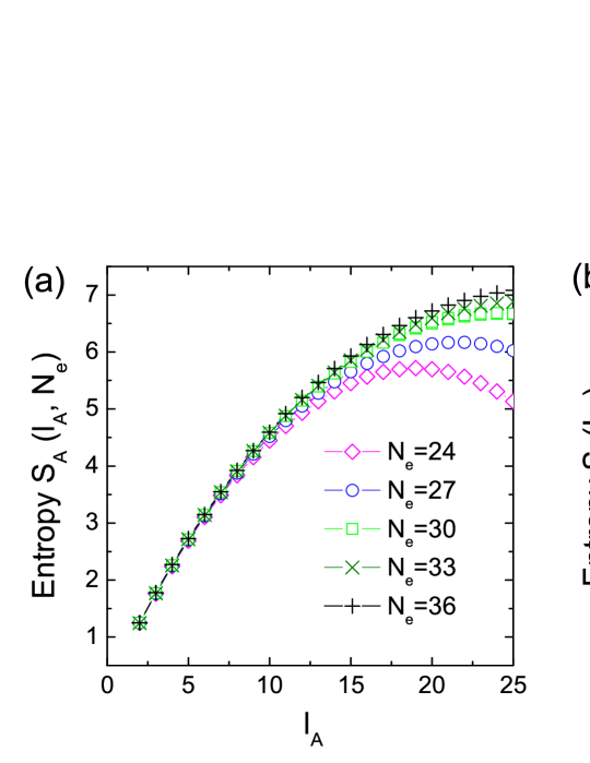
Figure 6: (a). Entanglement entropies with orbital partitioning $S(l_{A},N_{e})$, for various system sizes $N_{e}$, where $l_{A}\leq\frac{1}{2}N_{e}$ is the number of orbitals abive the cut in the northern hemisphere. (b). Scaling of entanglement entropies to $S(l_{A},N_{e}=36)=-\gamma+\alpha\sqrt{l_{A}}$ based on the solid circles (O the sphere, The length of the cut is proportional to $\sqrt{l_{A}}$ Haque2006). The dashed blue line is the theoretical $\text{RR}_{k=3}$ TEE value $\gamma\approx 1.447$. The open circles were discarded in the extrapolation because they represent very small subsystems ($l_{A}<5$) and violate the area law Haque2006; Estienne2014 and the finite-size saturation effect ($l_{A}>16$).

Appendix D IV. Topological Entanglement Entropy

For a two-dimensional gapped topologically-ordered state, the entanglement entropy $S_{A}(l_{A})$ for a subsystem A with a finite boundary length $l_{A}$ is given by $S_{A}(l_{A})=\alpha l_{A}-\gamma$, where the TEE $\gamma$ is related to the total quantum dimension $\mathcal{D}$ by $\gamma=\ln\mathcal{D}$ Kitaev2006 ; Levin2006 . Since $\mathcal{D}$ contains the information about the quasiparticle content, the TEE can determine whether a given topological phase belongs to the universality class of a given topological field theory.

Fig. 6(a) shows numerically-calculated orbital-cut entanglement entropy $S(l_{A},N_{e})$ as a function of the number of orbital ($l_{A}$) in the northern hemisphere for different system sizes ($N_{e}$). The initially-increasing parts of $S(l_{A},N_{e})$ reflect the physics of the macroscopic state, while the downward curvature is a finite-size effectHaque2006; Zozulya2007; Estienne2014. With the help of the DMRG, we can obtain reliable entropies for $l_{A}\leq 16$, because the entropy for a given $l_{A}\leq 16$ is nearly saturated as $N_{e}$ increases from $30$ to $36$, as shown in Fig. 6(a). In Fig. 6(b), we extract the TEE (red line), based on the raw data from $N_{e}=36$. The obtained TEE is $\gamma=1.491\pm 0.091$ (If we perform the extrapolation based on different system sizes, similar results are obtained: for example, for $N_{e}=33$, we get $\gamma\approx 1.519\pm 0.081$). This is consistent with the theoretical value $\ln\mathcal{D}=\ln\sqrt{5(1+\phi)}\approx 1.447$ for RR $k=3$ state, where each non-Abelian Fibonacci anyon quasiparticle sector contributes quantum dimension $d_{F}=\phi=(\sqrt{5}+1)/2$ ($\phi$ denotes the Golden Ratio). The appearance of $d_{F}=\phi$ is a signal of the emergence of Fibonacci anyon quasiparticles, indicating two Fibonacci quasiparticles may fuse into the identity or into one Fibonacci quasiparticle. This exotic property makes Fibonacci quasiparticles capable of universal quantum computation, where all the quantum gates can be operated and measured by braiding Fibonacci anyons Nayak .

Appendix E V. Entanglement spectrum at $\nu=12/5$

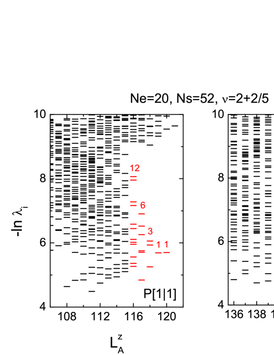
Figure 7: Orbital ES of the GS for partition $P[1|1]$ and $P[0|0]$ for FQH $\nu=12/5$ state. The system size is $N_{e}=20$ and $N_{s}=52$. The first four multplicity-patterns are labeled by numbers.

Here we show the entanglement spectrum for the groundstate at $\nu=2+2/5$, which is the particle-hole (PH) conjugate state of $13/5$ state. In spherical geometry, the highest density “root configuration” for the PH-conjugate RR $k=3$ state has a pattern of “0001100011000…11000”. Consequently, there are also two distinct ways of partitioning, with $2n-1$ (labeled as $P[1|1]$) and $2n$ ($P[0|0]$) electrons in the subsystem. In Fig. 7, we show the ES of two partitions for $N_{e}=20$. For $P[1|1]$ the leading ES displays the sequence of multiplicities $1,1,3,6,12$ in the first five momentum sectors $\Delta L=0,1,2,3,4$. For $P[0|0]$, ES shows the multiplicity pattern $1,2,5,9$ in the $\Delta L=0,1,2,3$ momentum sectors. The ES picture found is exactly the same as that of the $\nu=13/5$ state, taking into account PH conjugation so that $P[0|0]$ ($P[1|1]$) for $\nu=12/5$ relates to $P[1|1]$ ($P[0|0]$) for $\nu=13/5$. The low-lying ES structure is that predicted by the $SU(2)_{3}$ CFT for the RR $k=3$ state, and provides a fingerprint of the topological order for the groundstate at $\nu=12/5$.

Appendix F VI. Infinite DMRG on cylinder geometry

The main results in this paper have been obtained with finite DMRG calculations in spherical geometry. Spherical geometry simulations are efficient for calculating the groundstate energy and related neutral gap. The corresponding ES can also be obtained. Nevertheless, one drawback of spherical geometry is that one needs to select a “shift” value $\mathcal{S}$ in the calculation. Usually, this value is determined by some empirical knowledge of the model wavefunction or one needs to compare results using different shifts. Another disadvantage of spherical geometry is that the sphere has genus zero so that it is not suitable for discussing the topological degeneracy for topological ordered state.

An alternative strategy is to treat the cylinder geometry using ithe infinite DMRG algorithm Zatel2013 ; Zatel2015 ; McCulloch. Here, we briefly introduce our implementation of infinite DMRG. In the infinite-size DMRG, we first start from a small system size. Then we insert several orbitals (for $\nu=13/5$, we add ten orbitals each time) in the center, and optimize the energy by sweeping over the inserted orbitals. After the optimization, we absorb the new orbitals into the original existing system (here $5$ orbitals are added to the left system and $5$ to the right environment) and get the new boundary Hamiltonian. We repeat these insertion, optimizing and absorption procedures until both energy and entropy convergence are achieved by keeping a large number of states ($M$). There are some advantages of infinite DMRG over the finite DMRG. Compared with the finite DMRG simulation, infinite DMRG grows the system by several orbitals at each iteration and only sweeps the inserted part, thus the computational cost is significantly reduced. In the infinite DMRG algorithm, we do not need to set a “shift” $\mathcal{S}$ in the calculation. One can also access different topological sectors by randomizing the initial DMRG process. Details of the realization of infinite DMRG on cylinder geometry and the related benchmark for model Hamiltonian will be given elsewhere. Here we present some details related to the results shown in the main text.

Working on the cylinder geometry, we choose the Landau gauge $\vec{A}=(0,Bx)$, which conserves the y momentum around the cylinder. The single electron orbitals in N-th Landau level are:

$$\psi_{N,j}(x,y)=\left(\frac{1}{2^{N}N!\pi^{1/2}L_{y}l}\right)^{1/2}exp[i\frac{X_{j}}{l^{2}}y-\frac{(X_{j}-x)^{2}}{2l^{2}}]H_{N}(\frac{X_{j}-x}{l})$$ (4)

where $X_{j}=\frac{2\pi l^{2}}{L_{y}}j,j=1,2,\ldots,N_{s}$ is the center in x axis and $l$ is the magnetic length. $H_{N}(x)$ is the Hermite polynomial.

Introducing the destruction (creation) operator $a_{N,j}(a^{\dagger}_{N,j})$ for $\psi_{N,j}$, the Coulomb interaction can be written as

$$H_{C}=\sum\limits_{N_{1},\ldots,N_{4}}\sum\limits_{j_{1},..,j_{4}}V_{N_{1},j_{1},\ldots,N_{4},j_{4}}a^{\dagger}_{N_{1},j_{1}}a^{\dagger}_{N_{2},j_{2}}a_{N_{3},j_{3}}a_{N_{4},j_{4}}$$ (5)

where the Coulomb matrix elements are

$$V_{N_{1},j_{1},\ldots,N_{4},j_{4}}=\frac{1}{2}\int d\textbf{r}_{1}\int d\textbf{r}_{2}\psi^{*}_{N_{1},j_{1}}(\textbf{r}_{1})\psi^{*}_{N_{2},j_{2}}(\textbf{r}_{2})V(\textbf{r}_{1},\textbf{r}_{2})\psi_{N_{3},j_{3}}(\textbf{r}_{2})\psi_{N_{4},j_{4}}(\textbf{r}_{1})$$ (6)

If we only consider the second Landau level (setting $N_{i}=1$), we can rewrite the Hamiltonian as

$$H_{C}=\sum_{l}\sum\limits_{n\geq 0,m>0}V(m,n)a^{\dagger}_{l}a_{l+n}a_{l+m+n}a^{\dagger}_{l+m+2n}+h.c.,$$ (7)

where $V(m,n)$ is the matrix element derived from the modified Coulomb interaction. In this work, when studying on cylinder geometry, we choose the form of the modified Coulomb interaction as Zatel2015

$$V(\textbf{r}_{1},\textbf{r}_{2})=\frac{1}{|\textbf{r}_{1}-\textbf{r}_{2}|}e^{-\frac{(\textbf{r}_{1}-\textbf{r}_{2})^{2}}{\xi^{2}}}$$ (8)

This is the form suitable for DMRG calculations on the cylinder. In the implementation, we kept all Coulomb interaction terms $|V(m,n)|>10^{-6}$ within the truncated range $n<4\xi,m<\xi L_{y}/2$. We have checked that the physical quantities remain qualitatively unchanged when the truncation range is varied. Here we would like to point out that one of the important advantages of the infinite DMRG is that it can easily deal with this type of the Coulomb interaction in the cylinder geometry. In traditional finite-size DMRG in cylinder geometry, an additional one-body potential $U(x)$ is needed to avoid the electrons becoming trapped at the two ends of the finite cylinder, when studying the systems with Coulomb interaction between electrons. The infinite DMRG naturally overcomes this issue since it can access the actual results near the center by sweeping and edge effect should be suppressed when the length of the cylinder grows long enough to reach the fixed point for the state on the infinite cylinder.

To access the topologically different groundstates on cylinder using infinite DMRG, we repeatedly start the infinite DMRG simulation for a given system size $L_{y}$ for several times. In all calculations, we do not presume any empirical knowledge from model wavefunction. To be more explicit, we do not set a seed-state or an orbital configuration according to the root configuration in the initial DMRG process. We find that, in the relatively larger systems ($L_{y}\in[21,24]$), the system will automatically select one of the two groundstates $|\Psi_{1}\rangle$ and $|\Psi_{\phi}\rangle$ with almost equal probability. In the smaller system size ($L_{y}\in[18,20]$), the system has larger probability to fall into $|\Psi_{\phi}\rangle$ than $|\Psi_{1}\rangle$. In all cases, we have double checked both of the groundstates are stable and robust with changing the parameters in DMRG calculation. Once one groundstate has been developed, the groundstate is robust against increasing keep states or increasing the cylinder length in DMRG. For example, in Fig. 8, we show the entropy evolution of one groundstate in $|\Psi_{1}\rangle$ (red dots) and the other one in $|\Psi_{\phi}\rangle$ (black dots). The datas come from two independent infinite DMRG simulations. At the point marked by $M=8000$, we change the keep states from $m=7000$ to $m=8000$ and keep $m=8000$ for all steps after. The entropy of the two groundstates slightly increases with the increase of the keep states and the system length. There is no sign of tunnelling between the two groundstates in our infinite DMRG calculations. Physically, the tunnelling between two topological groundstates is forbidden since each topological groundstate hosts a well-defined anyonic flux line and the changing the global anyonic flux is energetically expensive. Furthermore, to check the two-fold groundstate degeneracy are complete, we try to start several infinite DMRG simulations with different random initializations. It is found that all simulations will randomly fall into $|\Psi_{\phi}\rangle$ or $|\Psi_{1}\rangle$. Thus we confirm the two-fold groundstates are indeed complete. Within randomizing the initial processes, although the two groundstates can be distinguished by characteristic orbital entanglement spectrum (as shown in main text), we find a small energy fluctuation and entropy fluctuation for each groundstate when we keep the same order of states in DMRG calculation. The entropy fluctuation is much smaller than the entropy difference $\Delta S\approx\ln\phi\approx 0.47$ between two topological sectors. We demonstrate the energy and entropy fluctuations as the error bars in Fig. 4(c-d) in the main text. The relatively larger uncertainty of entropy in system size $L_{y}\leq 20$ may result from: finite-size effect or that the groundstate at Coulomb point is very close to the phase boundary to a charge-density-wave (strip) state Rezayi2009 . To clarify the latter possibility, we measure the mean orbital occupation number $\langle n_{k}\rangle$ in the middle part of infinite cylinder. All of the groundstates have uniform occupation number with tiny fluctuation ($\Delta n_{k}<10^{-2}$).

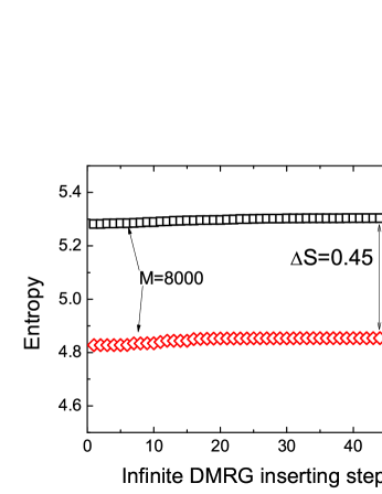
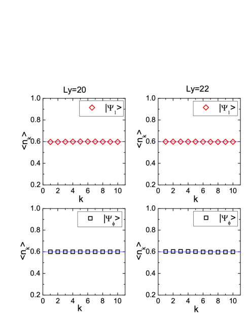
Figure 8: (Left) The entropy evolution of one groundstate realizing $|\Psi_{\phi}\rangle$ (black dots) and $|\Psi_{1}\rangle$ (red dots). These two groundstates come from two independent infinite DMRG simulations. We omit the infinite DMRG steps before we reach a nearly converged groundstate with keeping $M=7000$. We change the keep state from $M=7000$ to $M=8000$ at the point as arrow marked. Each infinite DMRG step means inserting ten orbitals in the middle of the cylinder and sweeping until entropy converged. Here the system size is $L_{y}=24l_{B}$. (Right) The mean orbital occupation number for two topological sectors on different system sizes. The dotted blue line shows $\nu=3/5$.

References

- (1) D. C. Tsui, H. L. Stormer, and A. C. Gossard, Phys. Rev. Lett. 48, 1559 (1982).
- (2) R. B. Laughlin, Phys. Rev. Lett. 50, 1395 (1983).
- (3) R. Willett, J. P. Eisenstein, H. L. Stormer, D. C. Tsui, A. C. Gossard, and J. H. English, Phys. Rev. Lett. 59, 1776 (1987).
- (4) W. Pan, J.-S. Xia, V. Shvarts, D. E. Adams, H. L. Stormer, D. C. Tsui, L. N. Pfeiffer, K. W. Baldwin, and K. W. West, Phys. Rev. Lett. 83, 3530 (1999).
- (5) J. S. Xia, W. Pan, C. L. Vicente, E. D. Adams, N. S. Sullivan, H. L. Stormer, D. C. Tsui, L. N. Pfeiffer, K. W. Baldwin, and K. W. West, Phys. Rev. Lett. 93, 176809 (2004),
- (6) H. C. Choi, et al., Phys. Rev. B 77, 081301(R) (2008).
- (7) W. Pan, et al., Phys. Rev. B 77, 075307 (2008).
- (8) A. Kumar, G. A. Csathy, M. J. Manfra, L. N. Pfeiffer and K. W. West, Phys. Rev. Lett. 105, 246808 (2010).
- (9) I. P. Radu, J. B. Miller, C. M. Marcus, M. A. Kastner, L. N. Pfeiffer, K. W. West, Science 320, 899 (2008).
- (10) M. Dolev, M. Heiblum, V. Umansky, A. Stern, and D. Mahalu, Nature 452, 829 (2012).
- (11) R. L. Willett, C. Nayak, K. Shtengel, L. N. Pfeiffer, and K. W. West, Phys. Rev. Lett. 111, 186401 (2013).
- (12) S. Baer, C. Rossler, T. Ihn, K. Ensslin, C. Reichl and W. Wegscheider, Phys. Rev. B 90, 075403 (2014).
- (13) C. Zhang, C. Huan, J. S. Xia, N. S. Sullivan, W. Pan, K. W. Baldwin, K. W. West, L. N. Pfeiffer, and D. C. Tsui, Phys. Rev B 85, 241302(R) (2012)
- (14) G. Moore and N. Read, Nucl. Phys. B 360, 362 (1991).
- (15) M. Greiter, X. G. Wen and F. Wilczek, Phys. Rev. Lett. 66, 3205 (1991).
- (16) N. Read and E. Rezayi, Phys. Rev. B 59, 8084 (1999).
- (17) C. Nayak, S. H. Simon, A. Stern, M. Freedman and S. D. Sarma, Rev. Mod. Phys. 80, 1083 (2008).
- (18) A. Y. Kitaev, Ann. Phys. 303, 2 (2003).
- (19) M. H. Freedman, M. Larsen, and Z. Wang, Commun. Math. Phys. 227, 605 (2002).
- (20) S. Das Sarma, M. Freedman and C. Nayak, Phys. Rev. Lett. 94, 166802 (2005).
- (21) L. Hormozi, G. Zikos, N. E. Bonesteel, and S. H. Simon, Phys. Rev. B 75, 165310 (2007).
- (22) N. E. Bonesteel, L. Hormozi, G. Zikos, and S. H. Simon, Phys. Rev. Lett. 95, 140503 (2005).
- (23) R. S. K. Mong, D. J. Clarke, J. Alicea, N. H. Lindner, P. Fendley, C. Nayak, Y. Oreg, A. Stern, E. Berg, K. Shtengel, and M. P. A. Fisher, Phys. Rev. X 4, 011036 (2014).
- (24) A. Vaezi and M. Barkeshli, Phys. Rev. Lett. 113 236804 (2014).
- (25) E. H. Rezayi and N. Read, Phys. Rev. B 79, 075306 (2009).
- (26) F. D. M. Haldane, Phys. Rev. Lett. 51, 605 (1983).
- (27) B. I. Halperin, Phys. Rev. Lett. 52, 1583 (1984).
- (28) J. K. Jain, Composite Fermions, (Cambridge Univeristy Press, Cambridge, England, 2007).
- (29) P. Bonderson and J. K. Slingerland, Phys. Rev. B 78, 125323 (2008).
- (30) P. Bonderson, A. E. Feiguin, G. Moller and J. K. Slingerland, Phys. Rev. Lett. 108, 036806 (2012).
- (31) G. J. Sreejith, C. Toke, A. Wojs and J. K. Jain, Phys. Rev. Lett. 107, 086806 (2011).
- (32) G. J. Sreejith, Y.-H. Wu, A. Wojs and J. K. Jain, Phys. Rev. B 87, 245125 (2013).
- (33) A. Wojs, Phys. Rev. B 80, 041104(R) (2009).
- (34) A. Kitaev and J. Preskill, Phys. Rev. Lett. 96, 110404 (2006).
- (35) M. Levin and X.-G. Wen, Phys. Rev. Lett. 96, 110405 (2006).
- (36) H. Li and F. D. M. Haldane, Phys. Rev. Lett. 101, 010504 (2008).
- (37) Y. Zhang, T. Grover, A. Turner, M. Oshikawa and A. Vishwanath, Phys. Rev. B 85, 235151 (2012).
- (38) X. G. Wen, Int. J. Mod. Phys. B 4, 239 (1990).
- (39) X. G. Wen, Advances in Physics 44, 405 (1995).
- (40) M. Haque, O. Zozulya, and K. Schoutens, Phys. Rev. Lett. 98, 060401 (2007).
- (41) A. M. Lauchli, E. J. Bergholtz, J. Suorsa and M. Haque, Phys. Rev. Lett. 104, 130502 (2010).
- (42) Z. Papic, B. A. Bernevig, and N. Regnault, Phys. Rev. Lett. 106, 056801 (2011).
- (43) L. Cincio and G. Vidal, Phys. Rev. Lett. 110, 067208 (2013).
- (44) M. P. Zaletel, R. S. K. Mong, F. Pollmann, Phys. Rev. Lett. 110, 236801 (2013).
- (45) H. H. Tu, Y. Zhang, and X. L. Qi, Phys. Rev. B 88, 195412 (2013).
- (46) H. C. Jiang, Z. H. Wang and L. Balents, Nat. Phys. 8, 902 (2012).
- (47) W. Zhu, S. S. Gong, F. D. M. Haldane, and D. N. Sheng, Phys. Rev. Lett. 112, 096803 (2014).
- (48) G. Fano, F. Ortolani, and E. Colombo, Phys. Rev. B 34, 2670 (1986).
- (49) M. Greiter, Phys. Rev. B 83, 115129 (2011).
- (50) S. R. White, Phys. Rev. Lett. 69, 2863 (1992).
- (51) T. Xiang, Phys. Rev. B 53, 10445(R) (1996).
- (52) N. Shibata and D. Yoshioka, Phys. Rev. Lett. 86 5755 (2001).
- (53) A. E. Feiguin, E. Rezayi, C. Nayak, and S. D. Sarma, Phys. Rev. Lett. 100, 166803 (2008).
- (54) J. Z. Zhao, D. N. Sheng and F. D. M. Haldane, Phys. Rev. B 83, 195135 (2011).
- (55) Z. X. Hu, Z. Papic, S. Johri, R. N. Bhatt, and P. Schmitteckert, Phys. Lett. A 376, 2157 (2012).
- (56) R. Morf, N. d‘Ambrumenil, and B. I. Halperin, Phys. Rev. B 34, 3037 (1986).
- (57) The charged gap is out of the scope of current study.
- (58) F. D. M. Haldane, and E. H. Rezayi, Phys. Rev. Lett. 54, 237 (1985).
- (59) S. M. Girvin, A. H. MacDonald and P. M. Platzman, Phys. Rev. Lett. 54, 581 (1985).
- (60) B. Yang, Z.-X. Hu, Z. Papic, and F. D. M. Haldane, Phys. Rev. Lett. 108, 256807 (2012).
- (61) While the obtained neutral gap is close to the experimental estimated value () at , the asymmetry between and in experiment Xia2004 ; Pan2008 is out of the scope of current paper, which is left for the future study.
- (62) E. J. Bergholtz and A. Karlhede, Phys. Rev. Lett. 94, 026802 (2005).
- (63) B. A. Bernevig and F. D. M. Haldane, Phys. Rev. Lett. 100, 246802 (2008).
- (64) B. A. Bernevig and F. D. M. Haldane, Phys. Rev. B 77, 184502 (2008).
- (65) M. R. Peterson, T. Jolicoeur, and S. Das Sarma, Phys. Rev. B 78, 155308(2008).
- (66) M. Storni, R. H. Morf, and S. Das Sarma, Phys. Rev. Lett. 104, 076803 (2010).
- (67) J. Biddle, M. R. Peterson, and S. Das Sarma, Phys. Rev. B 84, 125141 (2011).
- (68) K. Pakrouski, M. R. Peterson, T. Jolicoeur, V. W. Scarola, C. Nayak, and M. Troyer, Phys. Rev. X 5, 021004 (2015).
- (69) M. P. Zaletel, R. S. K. Mong, F. Pollmann and E. H. Rezayi, Phys. Rev. B 91, 045115 (2015).
- (70) J. Falson, D. Maryenko, B. Friess, D. Zhang, Y. Kozuka, A. Tsukazaki, J. H. Smet, and M. Kawasaki, Nat. Phys. 11, 347 (2015).
- (71) See the Supplemental Material for details.
- (72) The ES results shown in this paper give an unambiguous confirmation of RR3 state as the ground state at and . Based on this measurement, we can also exclude the possibility of the Jain CF state, because Jain state is expected to show degeneracy pattern in ES. Unfortunately, a direct exclusion of other candidates such as Bonderson-Slingerland (BS) state or bipartite CF state is unavailable, since it is still unknown the edge theory of these proposals. A further study of their excitations or edge theories will be necessary to distinguish between these proposals.
- (73) R. S. K. Mong, M. P. Zaletel, F. Pollmann and Z. Papic,, arXiv. 1505.02843.