Relativistic scaling laws for the light curve in supernovae

Abstract

In order to explain light curve (LC) for Supernova (SN) we derive a classical formula for the conversion of the flux of kinetic energy into radiation. We then introduce a correction for the absorption adopting an optical depth as function of the time. The developed framework allows to fit the LC of type Ia SN 2005cf ( B and V ) and type IIp SN 2004A (B,V,I and R ). A relativistic formula for the flux of kinetic energy is also derived in terms of a Taylor expansion and the application is done to the LC of GRB 050814. The decay of the radioactive isotopes as a driver the LC for SNs is also reviewed and a new formulation is introduced. The Arnett’s formula for bolometric luminosity is corrected for the optical depth and applied to SN 2001ay.

Keywords: supernovae: general, supernovae: individual (SN 2005cf), supernovae: individual (SN 2004A ), supernovae: individual (SN 2001ay), supernovae: individual (SN 1993J )

1 Introduction

The term light curve (LC) for Supernova (SN) usually denotes the behavior of the apparent/absolute visual magnitude as function of the time. The development of the multiwavelength astronomy fixes the wavelength passband, i.e BVRI, or the frequency $\nu$, i.e. 15.2 GHz, or the energy, i.e. 1kev. Further on in gamma, X and radio astronomies the flux or the count rate are recorded rather than the magnitude, see as an example Fong et al. (2012). The first model to be considered is connected with the radioactive decay

$$L=L_{\lambda,0}\exp(-\frac{t}{\tau_{n}})\quad,$$ (1)

where $L$ and $L_{\lambda,0}$ are the luminosities at time $t$ and at $t=0$ respectively, $\lambda$ is the considered wavelength and $\tau_{n}$ is the typical lifetime, see Bowers and Deeming (1984). On introducing the apparent magnitude $m_{\lambda}$, the previous formula becomes

$$m_{\lambda}=k^{\prime}_{\lambda}+1.0857(\frac{t}{\tau_{n}})\quad,$$ (2)

where $k^{\prime}_{\lambda}$ is a constant. The most important radioactive isotopes are ⁵⁶Ni with $\tau_{n}=8.757\,d$ and ⁵⁶Co with $\tau_{n}=111.47\,d$. The analysis of many authors has shown that the decay of one of these two radioactive isotopes fit only few days of a typical LC, see Smith and McCray (2007). At the same time the spectral index in the radio of SN 1993J  is constant after 700 days, see Figure 8 in Martí-Vidal et al. (2011) and this observational fact points toward the presence of synchrotron emission having flux , $F(\nu)\propto\nu^{-\alpha}$ with $\alpha\approx 0.7$. The hypothesis of the synchrotron emission in SNs is not new and we now report some applications among others: GRBs, see Preece et al. (2002); Beniamini and Piran (2013); Burgess et al. (2014) and Supernovae Remnants (SNRs), see Katsuda et al. (2010); Miceli et al. (2013). The presence of the synchrotron emission makes attractive the analysis of a turbulent cascade from the large scale to the small scales where presumably the relativistic electrons are accelerated. Insofar we have isolated two completely different physical mechanism for the source of radiation in the LC: (i) the number of radioactive isotopes as function of the time, (ii) the flux of mechanical kinetic energy which is the driver for the power injected in the turbulent cascade. The fact that the spectral index in the optical regime varies considerably with the time points toward a variable optical thickness as function of the time and of the considered pass-band. The basic idea is that the optical thickness is low at the beginning of the LC and it increases its value with time. A series of questions can now be posed

• Can we build a formula for the flux/magnitude versus time relationship in the framework of conversion of the mechanical luminosity into radiation?

• Can we introduce the correction for variable optical thickness introducing a dependence of the optical thickness with time?

• Can the new developed framework be applied to the various LCs which arise from the various typologies of LCs such as type Ia, Ib, Ic or type IIb, II-L, II-p, IIn?

• Can the radioactive model in it’s various versions model the most common LCs?

2 Preliminaries

Here we first introduce an elementary equation of motion and then we assume a linear relationship between the mechanical and the observed luminosity at a given frequency $\nu$.

2.1 The simplest equation of motion

The equation of the expansion of a SN in the first ten years can be modeled by a power law of the type

$$R(t)=R_{0}(\frac{t}{t_{0}})^{\alpha}\quad,$$ (3)

where $R$ is the radius of the expansion, $t$ is the time, $R_{0}$ is the radius at $t=t_{0}$ and $\alpha$ is an exponent which can be found from a numerical analysis. The velocity is

$$V(t)=\alpha R_{0}(\frac{1}{t_{0}})^{\alpha}t^{(\alpha-1)}\quad.$$ (4)

As an example in the case of SN 1993J  we have $\alpha$ = 0.828. The rate of transfer of mechanical energy, $L_{m}$ is

$$L_{m}(t)=\frac{1}{2}\rho(t)4\pi R(t)^{2}V(t)^{3}\quad.$$ (5)

We now assume that the density in front of the advancing expansion scale as

$$\rho(t)=\rho_{0}(\frac{R_{0}}{R})^{d}\quad,$$ (6)

where $d$ is a parameter which allows to match the observations; this assumption is not new and as an example Nagy et al. (2014) quotes d=3. The mechanical luminosity for the power law dependence of the radius becomes

$$L_{m}(t)=L_{0}(\frac{t}{t_{0}})^{5\alpha-d\alpha-3}\quad,$$ (7)

where $L_{0}$ is the luminosity at $t=t_{0}$.

2.2 The emitted radiation

The energy fraction of the mechanical luminosity, $L_{\nu}$, deposited in the frequency $\nu$ is assumed to be proportional to the mechanical luminosity through a constant $\epsilon_{\nu}$

$$L_{\nu}=\epsilon_{\nu}L_{m}\quad.$$ (8)

The flux at frequency $\nu$ and distance D is

$$F_{\nu}=\frac{\epsilon_{\nu}L_{m}}{4\pi D^{2}}\quad.$$ (9)

The problem of the absorption can be parametrized introducing a slab of optical thickness $\tau_{nu}$. The emergent intensity $I_{\nu}$ after the entire slab is

$$I_{\nu}=\int_{0}^{\tau_{\nu}}S_{\nu}e^{-t}dt\quad,$$ (10)

where $S_{\nu}$ is a uniform source function. The integration gives

$$I_{\nu}=S_{\nu}(1-e^{-\tau_{\nu}})\quad,$$ (11)

see formula 1.30 in Rybicki and Lightman (1991). A first model for the optical thickness assumes a power law dependence

$$\tau_{\nu}=a_{1,\nu}t^{a2,\nu}\quad,$$ (12)

where $a_{1,\nu}$ and $a_{2,\nu}$ are two coefficients which can be found from the astronomical data. The flux corrected for absorption in the power law case, $F_{\nu}$, is

$$F_{\nu,c}=\frac{\epsilon_{\nu}L_{m}}{4\pi D^{2}}(1-e^{-\tau_{\nu}})\quad.$$ (13)

An expression for the flux of the first model can be obtained inserting the simplest equation of motion for the $R-t$ dependence in the mechanical luminosity as given by (7)

$$F_{\nu,c}=F_{\nu,0}(\frac{t}{t_{0}})^{5\alpha-d\alpha-3}(1-e^{-\tau_{\nu}})\quad,$$ (14)

where $F_{\nu,0}$ is the flux a $t=t_{0}$. This formula is useful when we have the flux versus the time, as an example Jansky versus JD. The absolute/apparent magnitude version of for the first model is

$$m(t)=\frac{2.5\,\ln\left(t\right)\alpha\,d-12.5\,\alpha\,\ln\left(t\right)+7.5\,\ln\left(t\right)-2.5\,\ln\left(1-{{\rm e}^{-a_{{1}}{t}^{a_{{2}}}}}\right)}{\ln\left(2\right)+\ln\left(5\right)}+m_{k}\quad,$$ (15)

where $m_{k}$ is a constant of calibration. This formula is useful when we have the absolute/apparent magnitude versus time as in the case of optical LC in SN. The asymptotic approximation is

$$m(t)\sim 1.085\alpha d\ln\left(t\right)-5.428\alpha\ln\left(t\right)+3.257\ln\left(t\right)+m_{{k}}+\frac{0.542}{\left({{\rm e}^{{\frac{a_{{1}}}{\left({t}^{-1}\right)^{a_{{2}}}}}}}\right)^{2}}\quad.$$ (16)

A second model for the optical thickness assumes an exponential law dependence

$$\tau_{\nu}={\it a_{1,\nu}}\,\left(1-{{\rm e}^{-{\it a_{2,\nu}}\,{t}^{{\it a_{3,\nu}}}}}\right)\quad,$$ (17)

where $a_{1,\nu}$, $a_{2,\nu}$ and $a_{3,\nu}$ are three coefficients which can be found from the astronomical data. The absolute/apparent magnitude version for the second model is

$$m(t)=$$

$$\frac{2.5\ln\left(t\right)\alpha d-12.5\alpha\ln\left(t\right)+7.5\ln\left(t\right)-2.5\ln\left(1-{{\rm e}^{-a_{{1,\nu}}\left(1-{{\rm e}^{-a_{{2,\nu}}{t}^{{\it a_{3,\nu}}}}}\right)}}\right)}{\ln\left(2\right)+\ln\left(5\right)}$$ (18)

$$+m_{k}\,.$$

A third model for the optical thickness makes a comparison between the observed intensity $I_{obs}$ and the theoretical intensity $I_{th}$ through the optical depth

$$1-e^{-\tau_{\nu}}=\frac{I_{obs}}{I_{th}}\quad.$$ (19)

The optical depth is

$$\tau_{\nu}=-\ln(1-\frac{I_{obs}}{I_{th}})\quad.$$ (20)

The observed intensity as function of the time is an astronomical quantity and the theoretical intensity can be the mechanical luminosity or the momentary number of radioactive isotopes. Once the temporal behavior of $\tau_{\nu}$ is derived we search for the best fit as function of time. A fit already used is the power law fit as represented by eqn. (12). Another type of fit is the logarithmic polynomial approximation of degree M,

$$\tau_{\nu}(t)=a_{0}+a_{1}(\ln(t))+a_{2}(\ln(t))^{2}+\cdots+a_{M}(\ln(t))^{M}\quad.$$ (21)

The presence of the logarithm allows to cover the oscillatory behavior of $\tau_{\nu}$ over many decades in time.

3 Astrophysical results

The time is usually expressed in JD or seconds and a subtraction of the initial JD or seconds relative to the considered phenomena should be done in order to have zero at the beginning of the temporal scale. We start by analyzing SN 2005cf in NGC 5812 which is of type Ia, it’s distance is 29.4 Mpc and the distance moduli $\mu=32.51$, see Pastorello et al. (2007). Figure 1 reports the temporal evolution of the $V$ visual magnitude of SN 2005cf for the power law model as well the interpolating curve and Figure 2 the asymptotic approximation; data as in Table 1.

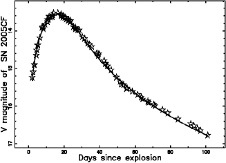
Figure 1: The $V$ LC of SN 2005cf (empty stars) and theoretical curve as given by the first model, see eqn. (15) (full line).

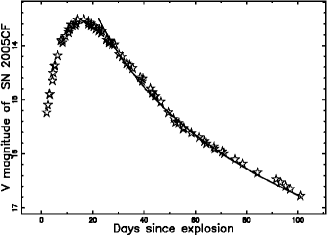
Figure 2: The $V$ LC of SN 2005cf (empty stars) and theoretical curve as given by the asymptotic formula (16), (full line).

The quality of the fits is measured by the merit function $\chi^{2}$

$$\chi^{2}=\sum_{j}{(m_{th}-m_{obs})^{2}}\quad,$$

where $m_{th}$ and $m_{obs}$ are the theoretical and observed magnitude, respectively.

Table 1: Numerical values of the adopted parameters and $\chi^{2}$ for the optical LC in SN in the case of optical thickness with a power law dependence, $\alpha=0.828$ everywhere.

Name  SN	band	d	$a_{1}$	$a_{2}$	$m_{k}$	$\chi^{2}$
SN 2005cf	V	3.80	1.9 $10^{-4}$	2.95	6.73	0.188
SN 2005cf	B	3.85	1.98 $10^{-4}$	3.2	7.11	6.7
SN 2004A	V	4.15	1.0 $10^{-4}$	4.15	5.33	12.4
SN 2004A	B	3.52	$2.6~{}10^{-3}$	1.85	9.53	2.50
SN 2004A	I	4.33	$2.0~{}10^{-5}$	2.65	3.4	0.35
SN 2004A	R	4.05	$7.8~{}10^{-5}$	2.3	4.81	1.10

Table 2: Numerical values of the adopted parameters and $\chi^{2}$ for the optical LC in the case of optical thickness with an exponential law dependence, $\alpha=0.828$ everywhere.

Name  SN	band	d	$a_{1}$	$a_{2}$	$a_{3}$	$m_{k}$	$\chi^{2}$
SN 2005cf	V	3.79	10	1.75 $10^{-5}$	3	6.73	0.202
SN 2005cf	B	3.81	5	8.2 $10^{-5}$	3	7.32	6.45
SN 2004A	V	4.36	10	6.27 $10^{-7}$	3	4.07	1.70
SN 2004A	B	3.79	100	$6~{}10^{-7}$	3	8.15	2.4
SN 2004A	I	4.67	2.5	$1.0~{}10^{-6}$	3.0	1.62	0.52
SN 2004A	R	4.23	10	$4.51~{}10^{-7}$	3	3.83	1.6

The (B–V) color evolution of SN 2005cf for the exponential law model (data as in Table 2) is reported in Figure 3.

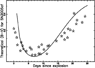
Figure 3: The (B–V) color evolution of SN 2005cf (empty stars) and the relative fitting straight line (full line). The theoretical curve is given by the second model. The time is limited to the first 25 days.

The SNs of type IIp are characterized by a flat LC for a long period of time, i.e. 100 days. We therefore analyzed SN 2004A in NGC 6207 , which is of type IIp, the distance is 25.6 Mpc and the distance moduli $\mu=31.99$, see Hendry et al. (2006); Tsvetkov (2008). Figure 4 reports the temporal evolution of the $V$ visual magnitude of SN 2004A for the exponential law model as well the interpolating curve, data as in Table 2.

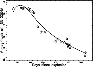
Figure 4: The $V$ LC of SN 2004A (empty stars) and theoretical curve as given by the second model, see eqn. (2.2) (full line).

We now apply the developed theory to model the radio flux density of SN 1993J  at 15.2 GHz, see Pooley and Green (1993); Ho et al. (1999), with data available at
http://www.mrao.cam.ac.uk/ dag/sn1993j.html . In this radio-case we plot the flux version of the first model as given by eqn.(14), see Figure 5 and Table 3.

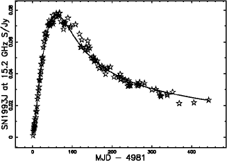
Figure 5: The radio flux density of SN 1993J  at 15.2 GHz (empty stars) and theoretical curve as given by the first model, see eqn. (14) (full line).

Table 3: Numerical values of the adopted parameters and $\chi^{2}$ for the radio LC in SN 1993J  and gamma LC in GRB 050814in the case of optical thickness with a power law dependence, $\alpha=0.828$ everywhere.

Name	band	d	$a_{1}$	$a_{2}$	$F_{\nu,0}$	$\chi^{2}$
SN 1993J	15.2 GHz	2.22	8.5 $10^{-4}$	1.86	1.64	7.9 $10^{-4}$
GRB 050814	0.2-10 kev	2.79	0.026	1.259	$8.3810^{-08}$	4.9 $10^{-18}$

The theory is now applied to GRB 050814at 0.3-10 kev in the time interval $10^{-5}-3$ days, see Jakobsson et al. (2006) with data available at
http://www.swift.ac.uk/xrt$\_$curves/00150314/. Figure 6 reports the LC, in this case the flux, as function of the elapsed time since Burst Alert Telescope (BAT) trigger and Table 3 reports the involved parameters.

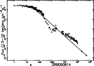
Figure 6: The XRT flux of GRB 050814at 0.2-10 kev (empty stars) and theoretical curve as given by the first model, see eqn. (14) (full line).

4 Relativistic model

The density, $\rho$, of the ISM at a distance $r$ from the SN is here modeled by a Lane–Emden ($n=5$) profile

$$\rho(r;b)=\rho_{c}{\frac{1}{{(1+\frac{{r}^{2}}{3b^{2}})^{5/2}}}}\quad,$$ (22)

where b represents the scale. The relativistic conservation of momentum for the thin layer approximation in presence of a the Lane–Emden ($n=5$) profile is given by the following differential equation

$$\frac{4\,{b}^{3}(r(t))^{3}\rho\,\pi\,\sqrt{3}{\frac{d}{dt}}r(t)}{(3\,{b}^{2}+(r(t))^{2})^{3/2}c\sqrt{-{\frac{({\frac{d}{dt}}r(t))^{2}}{{c}^{2}}}+1}}=\frac{4\,{b}^{3}{r_{{0}}}^{3}\rho\,\pi\,\sqrt{3}\beta_{{0}}}{(3\,{b}^{2}+{r_{{0}}}^{2})^{3/2}\sqrt{-{\beta_{{0}}}^{2}+1}}\quad,$$ (23)

where $r_{0}$ is the initial radius of the advancing sphere, $v_{0}$ is the initial velocity at $r_{0}$, c is the light velocity and $\beta_{0}=\frac{v_{0}}{c}$. The relativistic transfer of energy through a surface, $A$, is

$$L_{m,r}=A\gamma^{2}(\rho c^{2}+p)v\quad,$$ (24)

where $p$ is the pressure, for sake of simplicity we take p=0, and the Lorentz factor $\gamma$ is

$$\gamma=\frac{1}{\sqrt{1-\beta^{2}}dt}\quad,$$ (25)

see eqn. A31 in De Young (2002) or eqn. (43.44) in Mihalas and Mihalas (2013).

In the case of a spherical cold expansion

$$L_{m,r}=4\pi r(t)^{2}\frac{1}{1-\beta(t)^{2}}\rho(t)c^{3}\beta(t)\quad.$$ (26)

We now assume the following power law behavior for the density in the advancing thin layer

$$\rho(t)=\rho_{0}(\frac{t_{0}}{t})^{d}\quad,$$ (27)

and we obtain

$$L_{m,r}=4\pi r(t)^{2}\frac{1}{1-\beta(t)^{2}}\rho_{0}(\frac{t_{0}}{t})^{d}c^{3}\beta(t)\quad.$$ (28)

We can now derive $L_{m,r}$ in two ways: (i) from a numerical evaluation of r(t) and v(t), (ii) from a Taylor series of $L_{m,r}(t)$ of the type

$$L_{m,r}(t)=\sum_{n=0}^{3}a_{{n}}{(t-t_{0})}^{n}\quad.$$ (29)

The coefficients are

$$a_{0}= \frac{-4\,\pi\,{r_{{0}}}^{2}\left({\frac{t_{{0}}}{t}}\right)^{d}{c}^{3}\beta_{{0}}}{{\beta_{{0}}}^{2}-1}$$

$$a_{1}= \frac{4\,\pi\,r_{{0}}{c}^{4}{\beta_{{0}}}^{2}\left({\frac{t_{{0}}}{t}}\right)^{d}\left(9\,{b}^{2}{\beta_{{0}}}^{2}+3\,{b}^{2}-2\,{r_{{0}}}^{2}\right)}{\left(3\,{b}^{2}+{r_{{0}}}^{2}\right)\left({\beta_{{0}}}^{2}-1\right)}$$ (30)

$$a_{2}= \frac{2\,{\beta_{{0}}}^{3}{c}^{5}\left({\frac{t_{{0}}}{t}}\right)^{d}\pi\,\left(162\,{b}^{4}{\beta_{{0}}}^{4}-297\,{b}^{4}{\beta_{{0}}}^{2}-9\,{b}^{2}{\beta_{{0}}}^{2}{r_{{0}}}^{2}-45\,{b}^{4}+15\,{b}^{2}{r_{{0}}}^{2}-2\,{r_{{0}}}^{4}\right)}{\left(3\,{b}^{2}+{r_{{0}}}^{2}\right)^{2}\left({\beta_{{0}}}^{2}-1\right)}$$

$$a_{3}= \frac{18\,\left(270\,{b}^{2}{\beta_{{0}}}^{6}-675\,{b}^{2}{\beta_{{0}}}^{4}-33\,{\beta_{{0}}}^{4}{r_{{0}}}^{2}+480\,{b}^{2}{\beta_{{0}}}^{2}+62\,{\beta_{{0}}}^{2}{r_{{0}}}^{2}+45\,{b}^{2}-5\,{r_{{0}}}^{2}\right){\beta_{{0}}}^{4}{b}^{4}{c}^{6}\pi\,\left({\frac{t_{{0}}}{t}}\right)^{d}}{r_{{0}}\left(27\,{b}^{6}+27\,{b}^{4}{r_{{0}}}^{2}+9\,{b}^{2}{r_{{0}}}^{4}+{r_{{0}}}^{6}\right)\left({\beta_{{0}}}^{2}-1\right)}\quad.$$

Figure 7 compares the numerical solution for the luminosity and the series expansion for the luminosity about the ordinary point $t_{0}$.

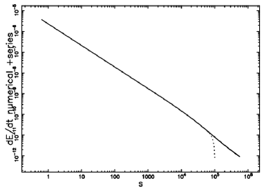
Figure 7: Numerical $L_{m,r}$ computed according to Eq. (28) (full line) and series solution as given by Eq. (29) (dotted line). Data as in Table 4.

Table 4: Numerical values of the parameters used in relativistic solutions.

$$\begin{array}[]{c}\hline\cr\hline\cr\vskip 3.0pt plus 1.0pt minus 1.0pt\cr parameters\\ t_{0}=2^{-8}~{}\mathrm{yr}~{}or~{}t_{0}=0.63~{}\mathrm{s}~{};r_{0}=0.00195~{}\mathrm{pc}~{};~{}\beta_{0}=0.833~{};~{}b=0.004~{}\mathrm{pc}\\ \vskip 3.0pt plus 1.0pt minus 1.0pt\cr\hline\cr\end{array}$$

The flux at frequency $\nu$ and distance $D$ is

$$F_{\nu,r}=\frac{\epsilon_{\nu}L_{m,r}}{4\pi D^{2}}\quad.$$ (31)

The flux corrected for absorption in the relativistic case is

$$F_{\nu,c,r}=\frac{\epsilon_{\nu}L_{m,r}}{4\pi D^{2}}(1-e^{-\tau_{\nu}})\quad.$$ (32)

As a behavior for ${\tau_{\nu}}$ as function of time we select a logarithmic polynomial approximation, see (eqn.21), of degree 9 and Figure 8 reports the flux of the relativistic LC as function of the elapsed time since Burst Alert Telescope (BAT) trigger.

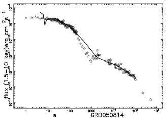
Figure 8: The XRT flux of GRB 050814at 0.2-10 kev (empty stars) and theoretical curve as given by the relativistic numerical model, see eqn. (32) (full line).

5 The radioactive model

Here we consider the decay of a radioactive isotope, a radioactive chain and the Arnett’s rule for the bolometric luminosity.

5.1 Decay of one element

The decay of a radioactive isotope is modeled by the following equation

$$-dN=\frac{N}{\tau_{n}}dt\quad,$$ (33)

where $\tau_{n}$ is a constant and the negative sign indicates that $dN$ is a reduction in the number of nuclei , see Yang and Hamilton (2010). The integration of this differential equation of the first order in which the variables can be separated gives:

$$N(t)=N_{0}e^{-\frac{t}{\tau_{n}}}\quad,$$ (34)

where $N_{0}$ is the number of nuclei at $t=0$. The half life is $T_{1/2}=ln(2)\;\tau_{n}$. The absolute magnitude version of the previous formula is

$$M=-C\;Log_{10}(N(t))={-\frac{t}{\tau_{n}}}+k\quad,$$ (35)

where $M$ is the absolute luminosity, $C$ and $k$ are two constants. This means that we are waiting for a straight line for the absolute magnitude versus time relationship. At the same time the observational fact that the spectral index in the radio varies considerably but becomes constant, $\beta\approx-0.7$, after $\approx$ 700 days, see Figure 8 in Martí-Vidal et al. (2011), asks the absorption.

5.2 Radioactive chains

The isotope ⁵⁶Ni is unstable and decays ($\tau_{1}$ = 8.757 d, $T_{1/2}$ =6.07 d) into ⁵⁶Co emitting gamma photons. The isotope ⁵⁶Co is unstable and decays ($\tau_{2}$ = 111.47 d, $T_{1/2}$ = 77.27 d) into ⁵⁶Fe through electron capture and $\beta$-decay. The decay rates of of the two species, species 1 is ⁵⁶Ni and species 2 is ⁵⁶Co, is modeled by the following equations

$${\frac{\rm d}{{\rm d}t}}N_{{1}}\left(t\right) =-{\frac{N_{{1}}\left(t\right)}{\tau_{{1}}}}$$ (36a)

$${\frac{\rm d}{{\rm d}t}}N_{{2}}\left(t\right) ={\frac{N_{{1}}\left(t\right)}{\tau_{{1}}}}-{\frac{N_{{2}}\left(t\right)}{\tau_{{2}}}}.$$ (36b)

The two solutions obtained inserting as initial conditions $N_{1}(0)=N_{0,1}$ and $N_{2}(0)=0$ are

$$N_{1} =N_{{0,1}}{{\rm e}^{-{\frac{t}{\tau_{{1}}}}}}$$ (37a)

$$N_{2} =\left({\frac{\tau_{{2}}N_{{0,1}}}{\tau_{{1}}-\tau_{{2}}}{{\rm e}^{-{\frac{t}{\tau_{{1}}}}+{\frac{t}{\tau_{{2}}}}}}}-{\frac{\tau_{{2}}N_{{0,1}}}{\tau_{{1}}-\tau_{{2}}}}\right){{\rm e}^{-{\frac{t}{\tau_{{2}}}}}}.$$ (37b)

The sum of the two species, N(t), is according to formula (8.5) in Rust et al. (2010)

$$N(t)=C_{1}\,N_{1}(t)+C_{2}\,N_{2}(t)\quad,$$ (38)

where $C_{1}$ and $C_{2}$ are two adjustable parameters. This linear sum is associated with the LC in SNs assuming that the $\gamma$-rays are thermalized in the ejecta and emerge in the various bands. The logarithmic form,M(t) , is associated with the magnitude evolution

$$M=\frac{MN}{MD}$$ (39)

where

$$MN=k\ln(2)+k\ln(5)-\ln(N_{{0,1}})$$

$$-\ln({\frac{1}{\tau_{{1}}-\tau_{{2}}}(C_{{2}}\tau_{{2}}{{\rm e}^{-{\frac{t}{\tau_{{2}}}}}}{{\rm e}^{{\frac{t(\tau_{{1}}-\tau_{{2}})}{\tau_{{1}}\tau_{{2}}}}}}+C_{{1}}{{\rm e}^{-{\frac{t}{\tau_{{1}}}}}}\tau_{{1}}-C_{{1}}{{\rm e}^{-{\frac{t}{\tau_{{1}}}}}}\tau_{{2}}-C_{{2}}\tau_{{2}}{{\rm e}^{-{\frac{t}{\tau_{{2}}}}}})})\quad,$$ (40)

where k is a constant and

$$Md=\ln(2)+\ln(5)\quad.$$ (41)

We plot the decay of the LC of SN 2001el  , which is of type Ia, adopting a distance modulus of 31.65 mag, see Krisciunas et al. (2003), the nuclear decay which according to equation (35) is a straight line, and the theoretical curve of the two species as represented by equation 39, see Figure 9.

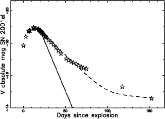
Figure 9: The $V$ LC of SN 2001el  (empty stars) in absolute magnitude, the theoretical curve as given by equation (35) when the radioactive decay of the isotope ⁵⁶Ni ($\tau_{n}$ = 8.757 d or $T_{1/2}$ =6.07 d , $k$=-18.65) was considered (full line), and the theoretical curve, (dashed line), connected with the decay of two species as represented by eq.(39) ($\tau_{1}=8.767d,\tau_{2}=111.477d,N_{0,1}=1$, $C_{1}$=1.9995, $C_{2}$=1.0005 and $k$=-18.4).

5.3 Bolometric luminosity

The bolometric LC after Arnett (1982); Arnett et al. (1985) has been associated with the combined radioactive decays of the isotopes ⁵⁶Ni and ⁵⁶Co. A formula of practical use is given by

$$L(t_{R})=\alpha\left((6.45\times 10^{43})e^{-t_{R}/8.8}+(1.45\times 10^{43})e^{-t_{R}/111.3}\right)\frac{erg}{s}\quad,$$ (42)

where $t_{R}$ is the elapsed time from the explosion to the maximum of the LC and $\alpha$ is $\approx$ 1, see formula (2) in Krisciunas et al. (2011). The previous formula represents the optically thin case. According to the comparison method developed in Section 2.2 a corrected bolometric luminosity for the absorption, $L_{c}(t_{R})$, is

$$L_{c}(t_{R})=L(t_{R})\times\left(1-{{\rm e}^{-a_{{1}}{t}^{a_{{2}}}}}\right)\quad,$$ (43)

and Figure 10 reports the comparison between observed and theoretical bolometric luminosity.

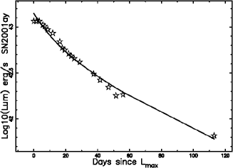
Figure 10: The bolometric LC of SN 2001ay  (empty stars) and the theoretical curve as given by eqn. (43) (full line). The parameters are $t_{R}$=22 days , $\alpha=1$ and the comparison method with a power law fit gives $a_{1}=105.88$ and $a_{2}=-1.335$. The astronomical data are extracted from Figure 18 in Krisciunas et al. (2011) by the author.

6 Conclusions

Classical and relativistic flux of energy: The classical flux of kinetic energy can be easily parametrized in the case of a radius-time relationship represented by a power law, see eqn.(7). Conversely is more complex to derive the relativistic flux of kinetic energy which requires a relativistic law of motion. In the framework of Lane–Emden ($n=5$) profile as given by eqn.(22) and momentum conservation in a thin layer we can deduce an analytical solution for the relativistic flux of energy in terms of a Taylor series, see the four coefficients in (30).

Light curve: Assuming a linear relationship between the luminosity in the various astronomical bands and the classical or relativistic flux of mechanical kinetic energy we can easily deduce a theoretical time dependence for the LC, see classical eqn.(9) or relativistic eqn.(29). This theoretical dependence is not enough and the concept of optical depth should be introduced. Among the infinite relationships for optical depth as function of time we selected a power law dependence, see eqn.(12), an exponential behavior, see eqn.(17), or a logarithmic polynomial approximation, see eqn.(21).

Nuclear Decay: The LC of a SN is often model by the decay of the radioactive isotope ⁵⁶Ni, but in order to follow the LC with time we should introduce a radioactive chain, see eqn. (38). Further on some classical approach to the bolometric luminosity must be corrected for the optical depth, see eqn.(43).

Comparison with astronomical data: The framework of conversion of the classical flux of mechanical kinetic energy into the various optical bands coupled with a time dependence for the optical depth allows to simulate the various morphologies of the LC: for a type Ia we chosen SN 2005cf, see Figure 1 for V band and Figure 3 for (B-V) color. The enigmatic behavior of type IIp SNs, here represented by SN 2004A, can also be modeled, see Figure 4 for the V band and Table 1 for B, I and R bands. The opposite sides of the electro-magnetic spectrum can also be simulated: for the radio band of SN 1993J  see Figure 5 and for the gamma/X spectrum of GRB 050814  see Figure 6. More complex is the derivation of the relativistic flux of energy here parametrized by a series expansion. The coupling of the previous series with a logarithmic polynomial approximation allows to model fine details such as the oscillation in LC visible at $\approx$ 1000 s in GRB 050814, see Figure 8. All the fits here presented report the $\chi^{2}$, see Tables 1 and 2. This means that other types of functions for the optical depth versus time have a reference for comparison.

References

- Arnett (1982) Arnett, W. D. (1982), “Type I supernovae. I - Analytic solutions for the early part of the light curve,” ApJ , 253, 785–797.
- Arnett et al. (1985) Arnett, W. D., Branch, D., and Wheeler, J. C. (1985), “Hubble’s constant and exploding carbon-oxygen white dwarf models for Type I supernovae,” Nature , 314, 337.
- Beniamini and Piran (2013) Beniamini, P. and Piran, T. (2013), “Constraints on the Synchrotron Emission Mechanism in Gamma-Ray Bursts,” ApJ , 769, 69.
- Bowers and Deeming (1984) Bowers, R. L. and Deeming, T. (1984), Astrophysics. I and II, Boston: Jones and Bartlett .
- Burgess et al. (2014) Burgess, J. M., Preece, R. D., Connaughton, V., Briggs, M. S., Goldstein, A., Bhat, P. N., Greiner, J., Gruber, D., Kienlin, A., Kouveliotou, C., McGlynn, S., Meegan, C. A., Paciesas, W. S., Rau, A., Xiong, S., Axelsson, M., Baring, M. G., Dermer, C. D., Iyyani, S., Kocevski, D., Omodei, N., Ryde, F., and Vianello, G. (2014), “Time-resolved Analysis of Fermi Gamma-Ray Bursts with Fast- and Slow-cooled Synchrotron Photon Models,” ApJ , 784, 17.
- De Young (2002) De Young, D. S. (2002), The physics of extragalactic radio sources, Chicago: University of Chicago Press.
- Fong et al. (2012) Fong, W., Berger, E., Margutti, R., Zauderer, B. A., and Troja, E. (2012), “A Jet Break in the X-Ray Light Curve of Short GRB 111020A: Implications for Energetics and Rates,” ApJ , 756, 189.
- Hendry et al. (2006) Hendry, M. A., Smartt, S. J., Crockett, R. M., Maund, J. R., Gal-Yam, A., Moon, D.-S., Cenko, S. B., Fox, D. W., Kudritzki, R. P., Benn, C. R., and Østensen, R. (2006), “SN 2004A: another Type II-P supernova with a red supergiant progenitor,” MNRAS , 369, 1303–1320.
- Ho et al. (1999) Ho, L. C., van Dyk, S. D., Pooley, G. G., Sramek, R. A., and Weiler, K. W. (1999), “Discovery of Radio Outbursts in the Active Nucleus of M81,” AJ , 118, 843–852.
- Jakobsson et al. (2006) Jakobsson, P., Levan, A., and Fynbo, J. P. (2006), “A mean redshift of 2.8 for Swift gamma-ray bursts,” A&A , 447, 897–903.
- Katsuda et al. (2010) Katsuda, S., Petre, R., Mori, K., Reynolds, S. P., Long, K. S., Winkler, P. F., and Tsunemi, H. (2010), “Steady X-ray Synchrotron Emission in the Northeastern Limb of SN 1006,” ApJ , 723, 383–392.
- Krisciunas et al. (2011) Krisciunas, K., Li, W., Matheson, T., and Howell, D. A. (2011), “The Most Slowly Declining Type Ia Supernova 2001ay,” AJ , 142, 74.
- Krisciunas et al. (2003) Krisciunas, K., Suntzeff, N. B., Candia, P., Arenas, J., Espinoza, J., Gonzalez, D., Gonzalez, S., Hoflich, P. A., Landolt, A. U., Phillips, M. M., and Pizarro, S. (2003), “Optical and Infrared Photometry of the Nearby Type Ia Supernova 2001el,” AJ , 125, 166–180.
- Martí-Vidal et al. (2011) Martí-Vidal, I., Marcaide, J. M., Alberdi, A., Guirado, J. C., Pérez-Torres, M. A., and Ros, E. (2011), “Radio emission of SN1993J: the complete picture. II. Simultaneous fit of expansion and radio light curves,” A&A , 526, A143+.
- Miceli et al. (2013) Miceli, M., Bocchino, F., Decourchelle, A., Vink, J., Broersen, S., and Orlando, S. (2013), “The shape of the cutoff in the synchrotron emission of SN 1006 observed with XMM-Newton,” A&A , 556, A80.
- Mihalas and Mihalas (2013) Mihalas, D. and Mihalas, B. (2013), Foundations of Radiation Hydrodynamics, Dover Books on Physics, New York: Dover Publications.
- Nagy et al. (2014) Nagy, A. P., Ordasi, A., Vinko, J., and Wheeler, J. C. (2014), “A semi-analytical light curve model and its application to type IIP supernovae,” ArXiv e-prints.
- Pastorello et al. (2007) Pastorello, A., Taubenberger, S., and et al (2007), “ESC observations of SN 2005cf - I. Photometric evolution of a normal Type Ia supernova,” MNRAS , 376, 1301–1316.
- Pooley and Green (1993) Pooley, G. G. and Green, D. A. (1993), “Ryle Telescope Observations of Supernova 1993J at 15-GHZ - the First 115 Days,” MNRAS , 264, L17.
- Preece et al. (2002) Preece, R. D., Briggs, M. S., Giblin, T. W., Mallozzi, R. S., Pendleton, G. N., Paciesas, W. S., and Band, D. L. (2002), “On the Consistency of Gamma-Ray Burst Spectral Indices with the Synchrotron Shock Model,” ApJ , 581, 1248–1255.
- Rust et al. (2010) Rust, B. W., O leary, D. P., and Mullen, K. M. (2010), “Modelling type Ia supernova light curves,” in Exponential Data Fitting and Its Applications, eds. Pereyra, V. and Scherer, G., Bentham Science Publishers, pp. 169–186.
- Rybicki and Lightman (1991) Rybicki, G. and Lightman, A. (1991), Radiative Processes in Astrophysics, New-York: Wiley-Interscience.
- Smith and McCray (2007) Smith, N. and McCray, R. (2007), “Shell-shocked Diffusion Model for the Light Curve of SN 2006gy,” ApJ , 671, L17–L20.
- Tsvetkov (2008) Tsvetkov, D. Y. (2008), “Photometric Observations of Two Type II-P Supernovae: Normal SN II-P2004A and Unusual SN 2004ek,” Peremennye Zvezdy, 28, 3.
- Yang and Hamilton (2010) Yang, F. and Hamilton, J. H. (2010), Modern atomic and nuclear physics, Hackensack, USA: World Scientific.