Statistical analysis of NOMAO customer votes for spots of France

Abstract

We investigate the statistical properties of votes of customers for spots of France collected by the startup company NOMAO. The frequencies of votes per spot and per customer are characterized by a power law distributions which remain stable on a time scale of a decade when the number of votes is varied by almost two orders of magnitude. Using the computer science methods we explore the spectrum and the eigenvalues of a matrix containing user ratings to geolocalized items. Eigenvalues nicely map to large towns and regions but show certain level of instability as we modify the interpretation of the underlying matrix. We evaluate imputation strategies that provide improved prediction performance by reaching geographically smooth eigenvectors. We point on possible links between distribution of votes and the phenomenon of self-organized criticality.

1 Introduction

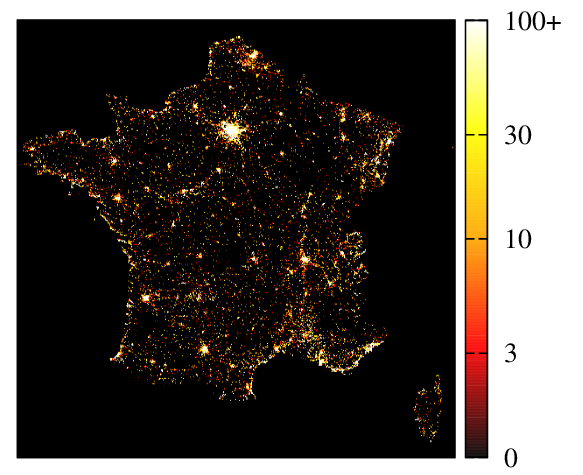
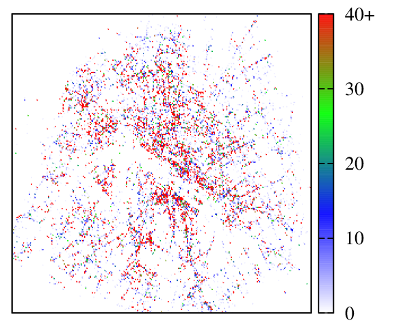
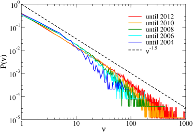
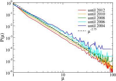
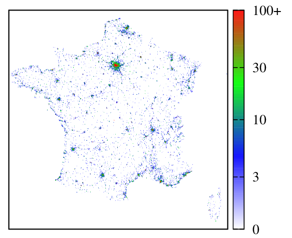
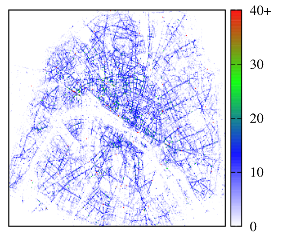
The young startup company NOMAO nomaocom collected a large database about customer (or user) votes for spots (or Points of Interest POIs or items) in France. The spots represent mainly restaurants and hotels with known geolocation coordinates. In this paper we investigate the statistical properties of these NOMAO votes and ratings of geolocalized items in a mix of geographic information and recommendations systems. The geographical distributions of votes are shown in Fig. 1 for the whole France and more specifically for Paris. The frequency distributions of votes per spot and votes per user are shown in Fig. 2 for France at different time intervals. It shows that these frequency distributions are stabilized in time and thus we are dealing with an unusual statistical system been at a certain steady-state. We note that at present a variety of real systems and networks are found to possess power law distribution (see e.g. dorogovtsev ) and thus here we investigate a new type of such a case with algebraic statistical properties.

Figure 1: Geographical distribution of votes for spots (POIs) in the original datasets. Top panel: case of France; (each square pixel represents $7.8{km}^{2}$); bottom panel: case of Paris (each square pixel represents $1370{m}^{2}$); color bars give a number of votes per pixel (cell), a limitation in number of votes is introduced for a better color representation.

To analyze the statistical properties of this real system we use the methods of recommender systems wikirecommender which gained a broad recognition in computer science after the Netflix Prize competition wikinetflix . In our research, distance, region and location become a side information over a multi-objective classification or regression problem. We concentrate on predicting user preferences by a spectral analysis based collaborative filtering that uses geo-location in addition to the ratings matrix.

We investigate how user taste, as described by latent factors, is reflected in the geographic information system. We compare the latent factors obtained by a full spectral analysis and by the stochastic gradient method, the standard recommendation technique wikirecommender applicable for matrices with a very large fraction of missed values.

The key difficulty in the spectral analysis lies in the abundance of missing values in the rating matrix: our matrix consists of 99.5% missing values while the Netflix matrix for example is 99% unknown. Several early results describe expectation maximization based singular value decomposition (SVD) algorithms, dating back to the seventies gabriel79weights and canny02collaborative ; srebro03weighted ; zhang05svd , describe the method for a recommender application.

A successful implementation of spectral analysis in recommender matrices with only a few known elements is described by Simon Funk in funk06netflix . His method is a variant of Stochastic Gradient Descent (SGD) reminiscent of gradient boosting friedman99gradient . SGD computes no eigenvalues and does not guarantee the orthogonality of the matrix factors. On the other hand, regularization is easily incorporated in SGD, which enables a better handling of the very large amount of missing values in the matrix and in particular, prevents overfit to training elements and provide better quality predictions of the unknown ratings.

In this paper, after describing methods and related results (Section 2) and the NOMAO data sets (Section 3), we compare and visualize the geo-localization of the matrix factors defined by SVD and SGD under various parameter settings in Section 4. We show that by imputing ratings to nearby locations we may form factors that yield a better description of the ratings matrix in Section 5.

Figure 2: Differential frequency distributions of votes for the case of France for different time intervals until year 2004, 2006, 2008, 2010, 2012. Top panel: differential probability $P(\nu)$ to have $\nu$ votes for spots (POIs); bottom panel: differential probability $P(\mu)$ to have $\mu$ votes per user (customer). Here the dashed lines show an average algebraic decay with exponents $a=1.5$ (top), $b=2.75$ (bottom).

2 Methods and related results

Recommenders based on the rank $k$ approximation of the rating matrix with the first $k$ singular vectors are probably first described in billsus98collaborative ; pryor98svd ; gupta99jester ; sarwar00application and many others near year 2000.

The Singular Value Decomposition (SVD) of a rank $\rho$ matrix $R$ is given by $R=U^{T}\Sigma V$ with $U$ an ${m\times\rho}$, $\Sigma$ a ${\rho\times\rho}$ and $V$ an ${n\times\rho}$ matrix such that $U$ and $V$ are orthogonal. By the Eckart-Young theorem GolubVanLoan the best rank-$k$ approximation of $R$ with respect to the Frobenius norm is

$$||R-U^{T}_{k}\Sigma_{k}V_{k}||_{F}^{2}=\sum_{ij}(r_{ij}-\sum_{k}\sigma_{k}u_{ki}v_{kj})^{2},$$ (1)

where $U_{k}$ is an ${m\times k}$ and $V_{k}$ is an ${n\times k}$ matrix containing the first $k$ columns of $U$ and $V$ and the diagonal $\Sigma_{k}$ containing first $k$ entries of $\Sigma$.

The rmse differs from the above equation only in that summation is over known ratings

$$\hbox{{rmse}}{}^{2}=\sum_{ij\in\text{known}}\mbox{err}_{ij}^{2}\mbox{ where }\mbox{err}_{ij}=r_{ij}-\sum_{k}\sigma_{k}u_{ki}v_{kj}.$$ (2)

Early works sarwar00application used SVD for recommenders by defining various strategies for handling the missing values in the rating matrix $R$ kurucz07spectral . The most natural idea is to impute the missing elements by zeroes, averages, or even repeatedly re-fill by predictions. It has turned out that all above missing value imputation methods overfit to the imputed values kurucz07spectral . More recent results emphasize the importance of regularization to avoid overfitting bell2007lnp ; takacs2008investigation . For this reason, the recommender systems community turned away from SVD and use other optimization methods for rating matrices with missing values, most notably stochastic gradient descent takacs2008unified and alternating least squares koren2009matrix .

In our problem, locality is an additional information that can be exploited for analyzing the recommender matrix. Surveys on recommendations in location-based social networks bao2013survey ; symeonidis2014location combine spatial ratings for non-spatial items, nonspatial ratings for spatial items, and spatial ratings for spatial items levandoski2012lars . Flickr geotags are used for travel route recommendation, concentrating on routes and not individual places in kurashima2010travel . User similarity based methods may combine friendship information with the distance of the user home locations ye2010location ; ye2011exploiting .

Most similar to our method is the Probabilistic Matrix Factorization approach that fuses geographic information cheng2012fused and observes that “users tend to check in around several centers, where the check-in locations follow a Gaussian distribution at each center […and] the probability of visiting a place is inversely proportional to the distance from its nearest center; if a place is too far away from the location a user lives, although he/she may like that place, he/she would probably not go there.”

3 The Nomao Datasets

Nomao is a startup company located in France nomaocom . It performs the analysis of point of interest (POI) rating and reservation services and collects POI information including user ratings from France with a special accent on Paris and Toulouse regions where the company headquarters are located. The Nomao dataset used in our experiments contain user-POI ratings, and GPS information of the rated POIs. We investigate two separated datasets. The first one contains information on POIs in France, while the second has ratings only on POIs located in Paris. We analyze the datasets collected during the time period up to year 2012.

Table 1 (top) shows the basic attributes of the original datasets. The average number of ratings per item is relatively large, the average number of ratings per user is very low. Moreover, only a very few percent of all user-item scores is known.

The distribution $P(\nu)$ of frequency of votes per spot $\nu$ (or item $i$) for France dataset is shown in the top panel of Fig. 2. This distribution is stable in time and is well described by the power law $P(\nu)\propto 1/\nu^{a}$ with $a\approx 1.5$. Also, the distribution $P(\mu)$ of frequency of votes per customer $\mu$ (or user $u$) remains stable in time with the power law dependence $P(\mu)\propto 1/\mu^{b}$ with $b\approx 2.75$. It is important to note that these distributions remain stable from year 2004 up to year 2012 even if the number of votes increases almost by two orders of magnitude during this period. At the moment we cannot provide theoretical reasons for the values of these exponents.

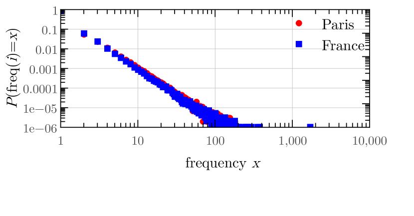
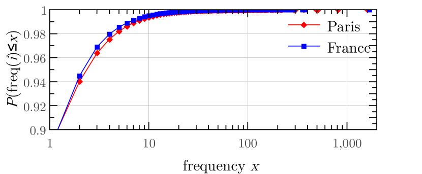
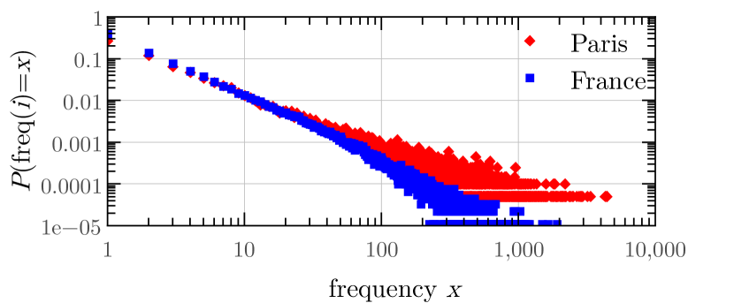
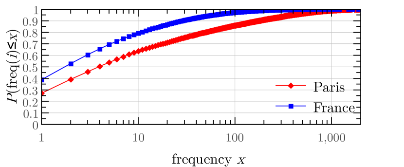
We call user activity how many times a user scored different items. We define item activity similarly. Fig. 3 shows the probability density function (PDF), an the cumulative density function (CDF) of user activities. Fig. 4 shows the same distributions for items. Both user and item activities follow power-law distributions with the exponent values being very similar for France and Paris datasets. As in Fig. 2 we find that the exponent for probability of votes for POIs is $a\approx 1.5$ while the exponent for the exponent for probability of votes of users is $b\approx 2.75$.

To handle the extreme sparsity of the user-item matrices, we selected a smaller subset of the user-item rating datasets by the following selection criteria:

• We only used ratings between 0-5. Part of the ratings, probably originating from a different system, were out of this range.

• We filtered out users and items that have less than $A$ ratings. In other words, we selected the subgraph of the user-item rating bipartite graph with users and items that have degree at least $A$. For Paris we set $A=10$, for France we set $A=5$.

Table 1 (bottom) shows the attributes of the selected subsets. In what follows we use these datasets in our experiments.

Table 1: Attributes of the original (top), and cleaned (bottom) datasets.

original	Paris	France
Number of ratings	1,539,964	1,432,601
Number of users	998,127	1,077,568
Number of items	20,576	99,976
Average ratings per user	1.543	1.329
Average ratings per item	74.84	14.32
Ratio of known ratings	0.0075%	0.0013%
cleaned	Paris	France
Number of ratings	114,352	97,452
Number of users	5,756	9,471
Number of items	2,952	7,605
Average ratings per user	19.87	10.29
Average ratings per item	38.74	12.81
Ratio of known ratings	0.672%	0.135%
Average rating	3.714	3.747

Figure 3: Probability density function (top), and cumulative density function (bottom) of user activities in the original datasets.

Figure 4: Probability density function (top), and cumulative density function (bottom) of item activities in the original datasets.

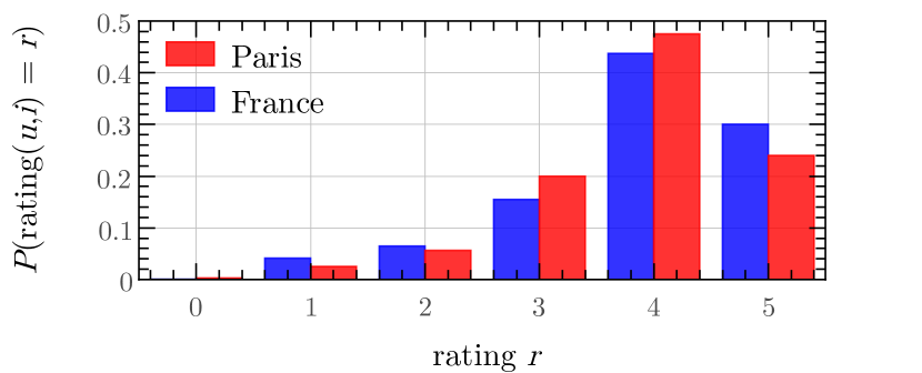
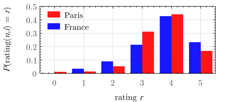
In Fig. 5 we show the score distributions: the top (bottom) panel shows the distributions for the original (cleaned) datasets. We see that the original and cleaned datasets have similar distributions of scores.

Fig. 6 shows the geographical density of POIs in France (top) and Paris (bottom) for the original datasets. The geolocation data of POIs are used in the following Sections for spectral analysis.

In the following we perform all computations with the cleaned datasets since the analysis of multiple votes of the same user provides more reliable statistical data.

Figure 5: Score distributions with integer binning. Top: original dataset, Bottom: cleansed dataset.

Figure 6: Geographical distribution of POIs in the original datasets. Top panel: case of France (each square pixel represents $7.8{km}^{2}$); bottom panel: case of Paris (each square pixel represents $1370{m}^{2}$); color bars give number of POIs per pixel (cell); a limitation in number of POIs is introduced for a better color representation.

4 Spectra of recommender matrices

4.1 Singular value decomposition

The recommender matrix $R$ consists of the preference values $r(u,i)$ of users $u$ for items $i$. The values may denote explicit rating values, e.g. 1-5 stars for Netflix movies bell2007lnp . We may also consider the so-called implicit ratings problem, where the value is 1 if the user visited POI $i$ and 0 otherwise. The value of the explicit matrix is missing whenever the user gave no rating yet. In most of the cases, this matrix is very sparse with only 1% or less known values. The implicit matrix is always a full 0–1 matrix, however the 0 values are uncertain: the user may not know about the item or had no time yet to visit it.

The so-called Latent Factor Model is an approximation $\hat{R}$ of the original rating matrix $R$,

$$\hat{r}(u,a)=\sum_{f=1}^{k}p_{uf}q_{af},$$ (3)

where $P=[p_{uf}]$ and $Q=[p_{uf}]$ are the user and item factor models, respectively.

For a fixed number of factors $k$, $\hat{r}$ approximates $r$ with the smallest root mean squared error if it is defined by the singular vectors corresponding to the $k$ largest singular values,

$$\hat{r}(u,a)=\sum_{f=1}^{k}p_{uf}q_{af},$$ (4)

where the singular value decomposition (SVD) of $R$ is $U\Sigma V^{T}$.

Since

$$RR^{T}=U\Sigma^{2}U^{T}\mbox{ and }R^{T}R=V\Sigma^{2}V^{T},$$ (5)

the spectrum of the recommender matrix $R$ is defined identically by the square root of the eigenvalues of $RR^{T}$ or $R^{T}R$. These latter matrices are symmetric positive semidefinite, the spectrum is non-negative real.

If $R$ contains missing values such as in the case of an explicit rating matrix, SVD is undefined. We may still define the best root mean square approximation by summing the error for the known ratings only as in equation (1).

4.2 Stochastic gradient descent: Latent factor modeling with missing values

We use the regularized matrix factorization method of takacs2008investigation and optimize the minimum squared error of the $k$-factor model

$$\hat{r}(u,i)=\sum_{l=1}^{k}p_{ul}q_{il},$$ (6)

where $p$ and $q$ contain the user and item models, respectively. By adding regularization with weight $\lambda$, we optimize the quantity

For a single event $(u,i)$ we optimize the coefficients $p_{ul}$ and $q_{il}$ for $l=1$, $\ldots$, $k$ by gradient descent with learning rate lrate as

(8)

(9)

Unlike SVD where eigenvalues are sorted, the SGD factors are not ordered by the above equations. In order to produce the eigenvector maps, we built ranked factors by an iterative SGD that optimize only on a single factor at a time funk06netflix .

4.3 Mapping SVD and SGD latent factors

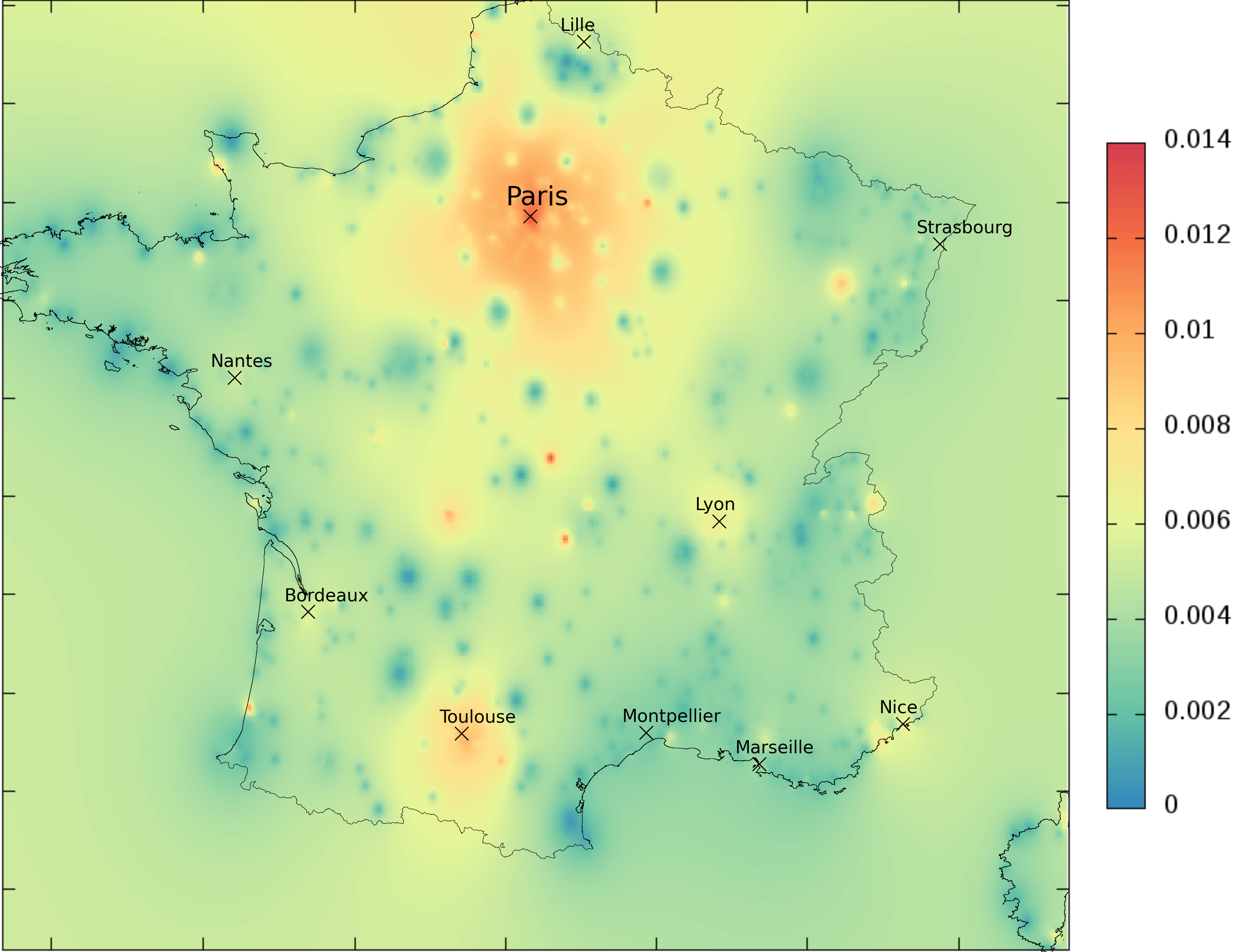
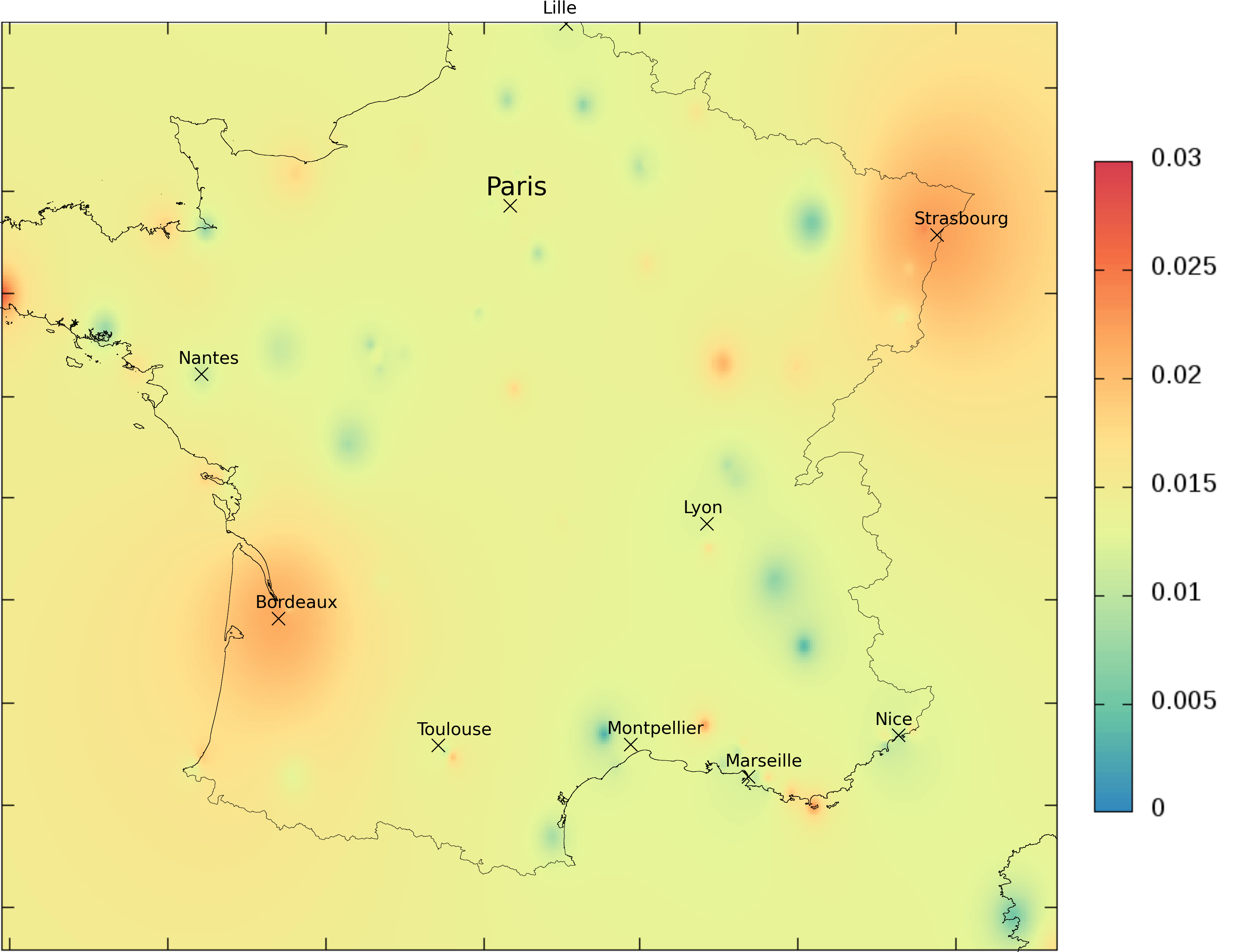
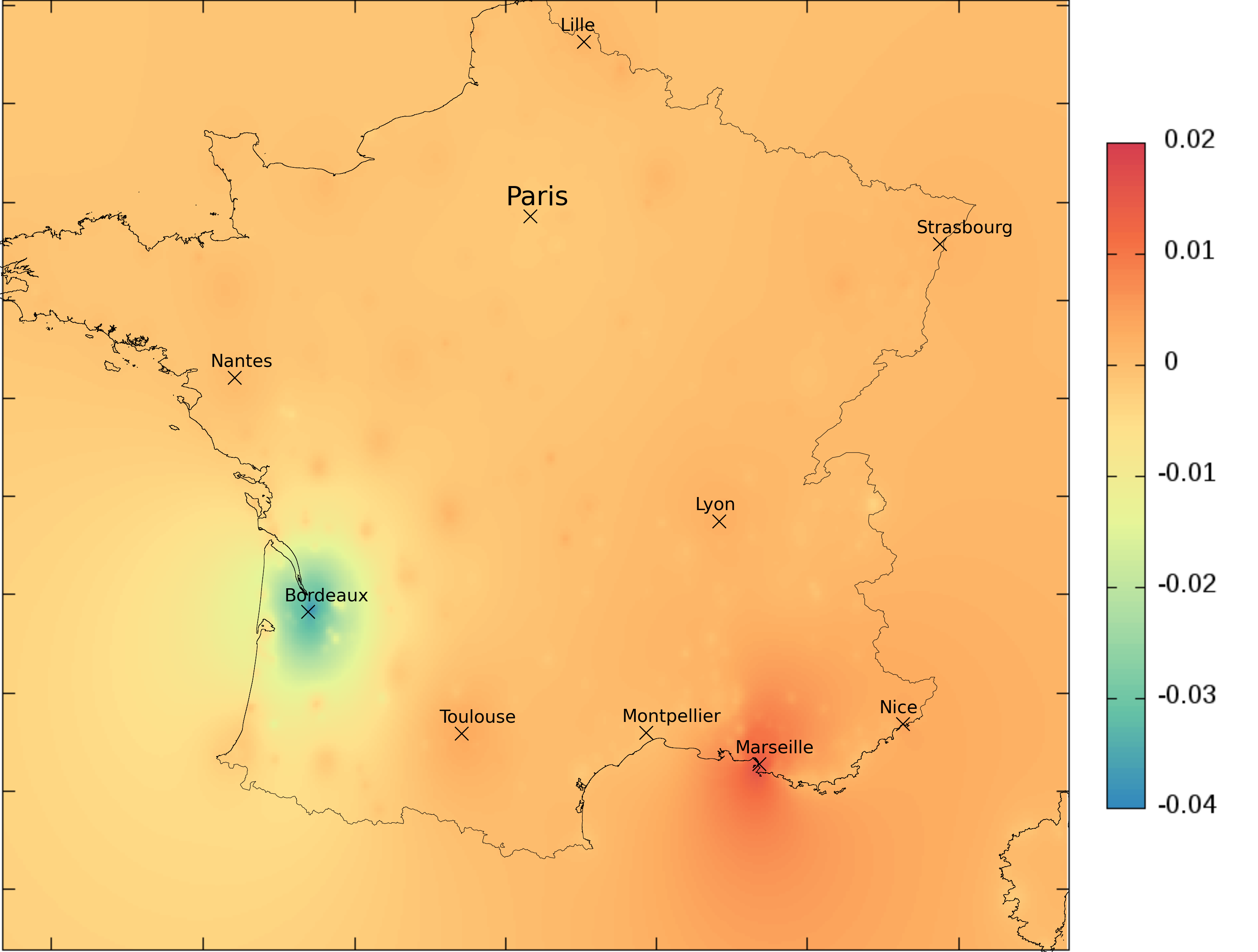
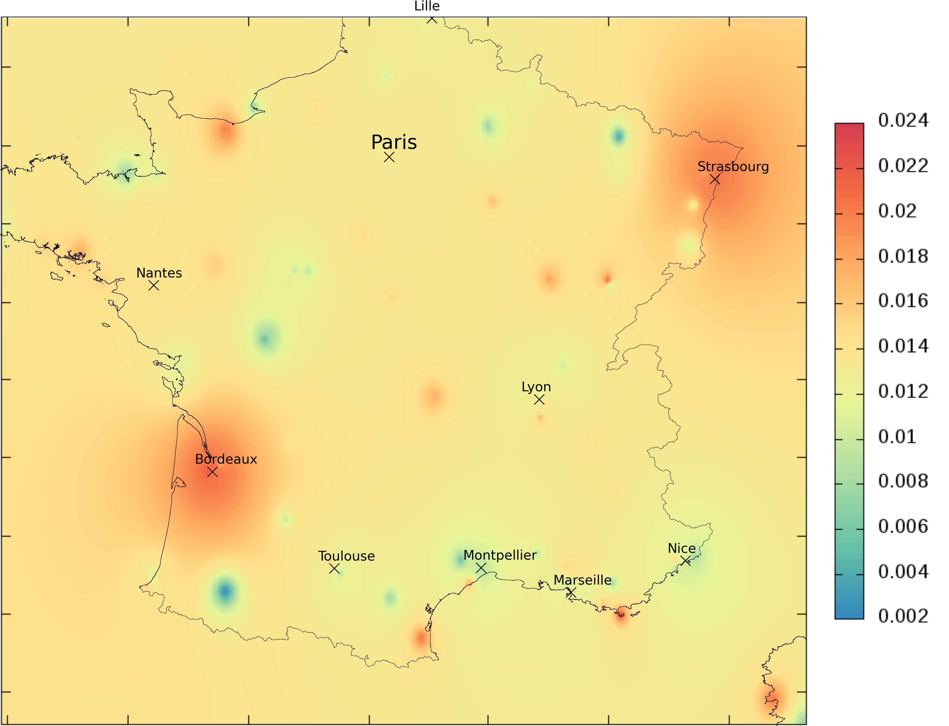
First we set each unknown value of $R$ to zero and computed the SVD decomposition. The first, second, and fourth singular vectors are plotted over the map of France (Fig. 7, left) by assigning the value in the vector to the location of the POI. More specifically, we averaged these values on a grid to create the final heatmaps. The smoothing algorithm weighted the value of each POI to the closest grid point inversely proportional to their euclidean distance.

The heatmaps in Fig. 7, left, indicate that the singular vectors are strongly geolocation related. The first few dimensions correspond to the largest cities in France.

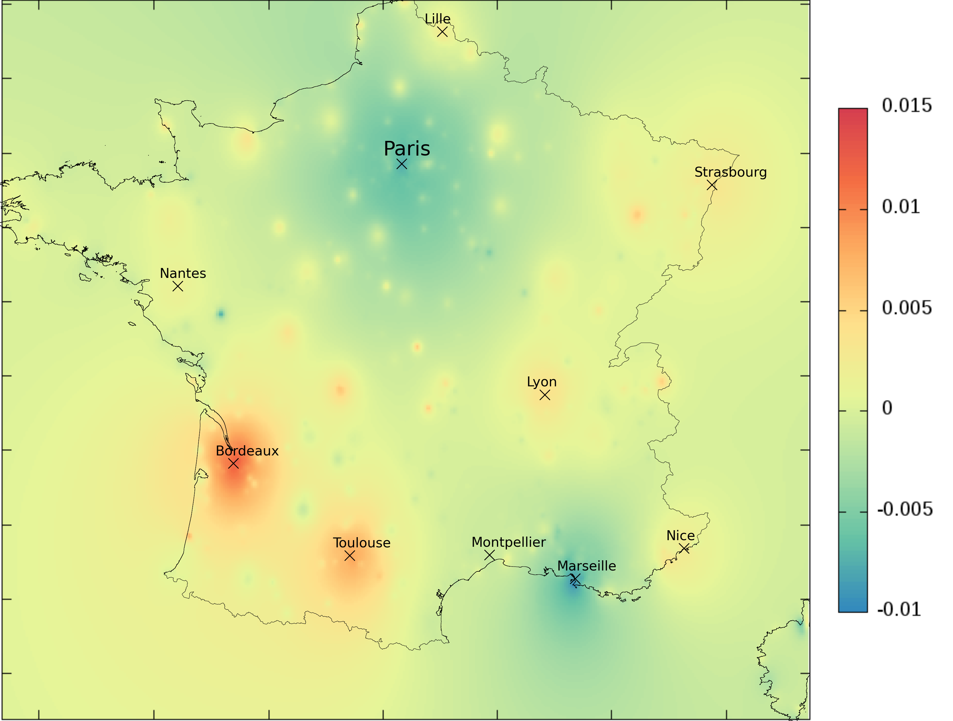
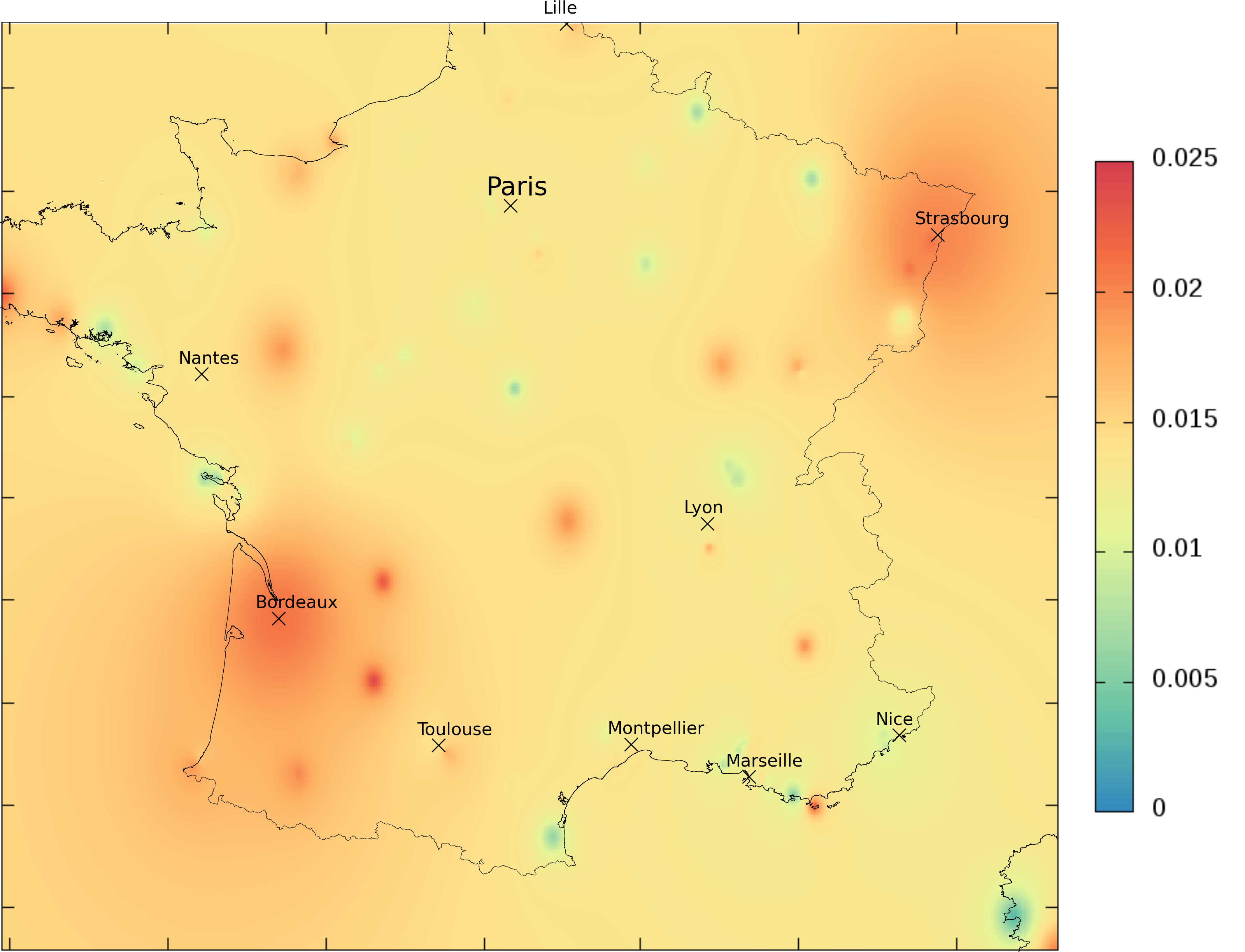
Similarly, we investigated the latent vectors of $R$ computed with the SGD algorithm. The first, second and fourth latent vectors are plotted over the map of France in Fig. 7, right, similar to the SVD eigenvectors. While the SVD singular vectors were centralized one-by-one on a large city, the SGD latent factors are the linear combination of them. The latent factors are also geolocation related, but not separated among the main cities like the SVD singular vectors.

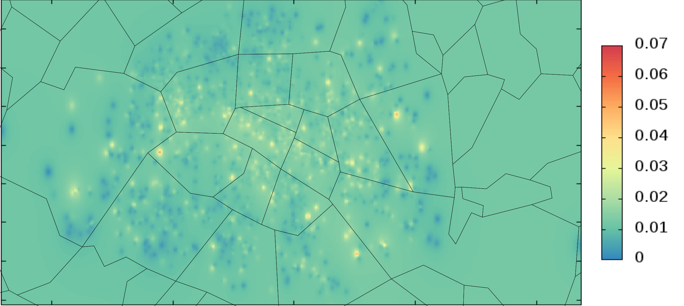
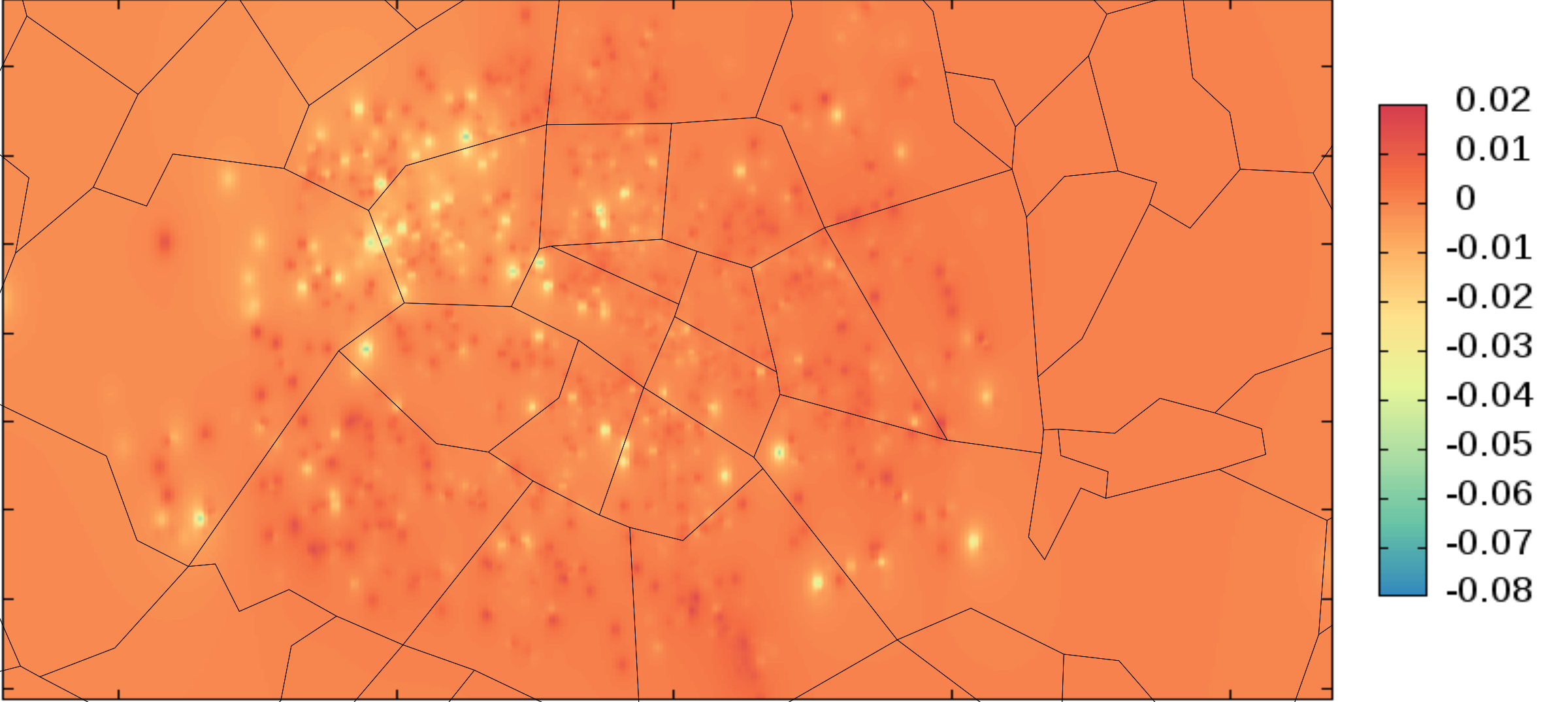
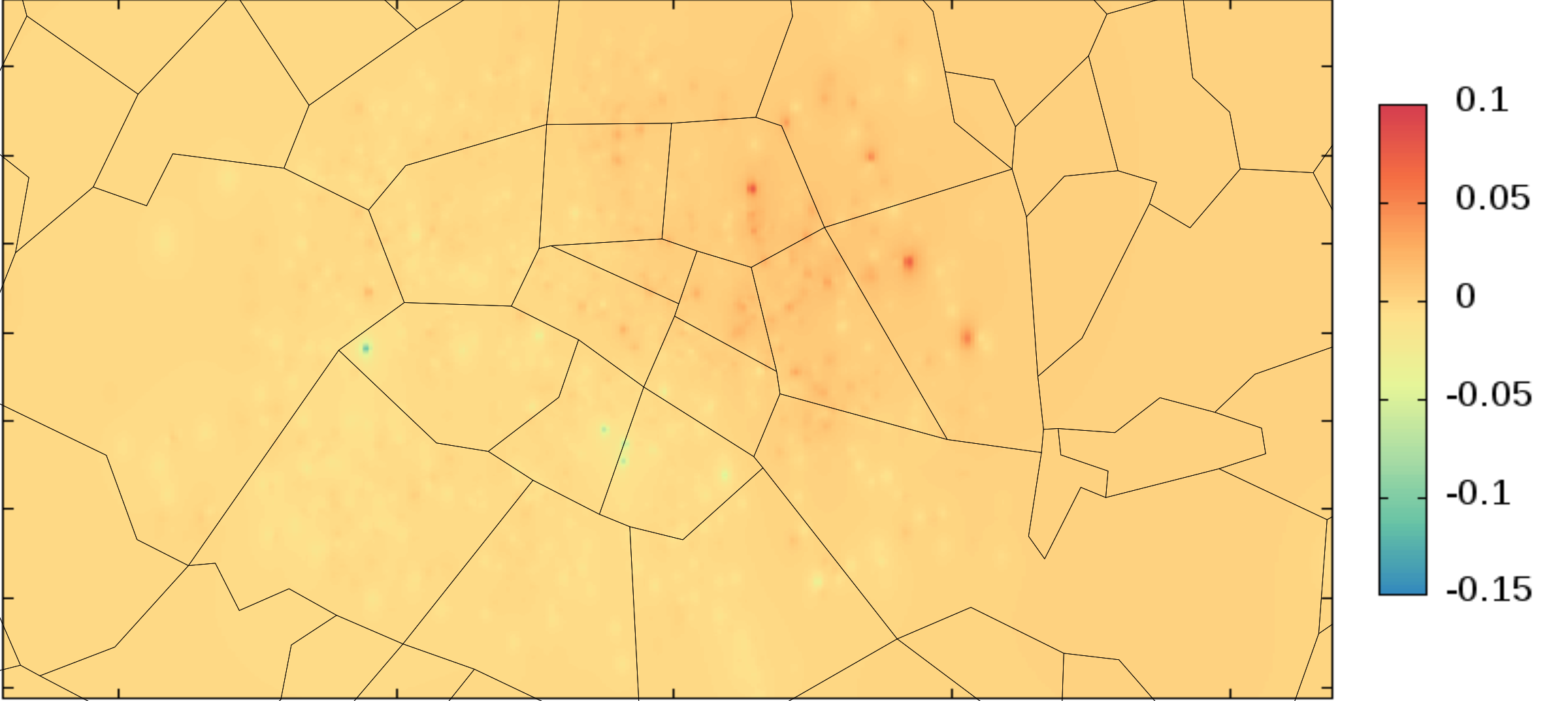
In 8 we mapped the first three singular vectors of the Paris dataset. The different vectors may focus on different districts. However, they are not as clearly separated as the singular vectors of the France dataset.

In Section 5 we use these key observations to improve the recommendation quality of the SGD.

Figure 7: The first, second and fourth singular vectors of the Nomao France rating matrix by SVD (left) and SGD (right). Here, the SVD eigenvectors correspond to Paris and Toulouse; Bordeaux, Toulouse and Marseille; Bordeaux and Marseille respectively, while the SGD plots for respective vectors are scattered around several cities.

5 Prediction for ratings and visits to locations

5.1 Recommender evaluation

Recommender systems serve to find new products for the users that are relevant for them. More specifically, for a given user $u$ an item $i$ a recommender system may retrieve the predicted relevancy $\hat{r}_{ui}$. This is called the rating prediction task. The Netflix Prize competition netflix-prize was a challenge in rating prediction. While in the Netflix Prize competition, contestants were optimizing to predict all ratings to the users, a recommender system in practice selects the top rated items for a given user. In this top-$K$ prediction task deshpande2004item ; cremonesi2010performance ; yuan2011factorization , a recommender system should retrieve for a given user a top list of items with length $K$. The top list should contain the most relevant items for the given user. This problem is more application related than the rating prediction task. In our experiments we examine both problems on the NOMAO datasets.

In addition to RMSE defined by equations (1) for full and (2) for partial matrices, we use two measures that evaluate the accuracy of the top-$K$ recommendation task.

Figure 8: The first, third and fourth singular vectors of the Nomao Paris rating matrix obtained by SVD.

Recall at $k$ is defined as the number of relevant POIs among the highest $k$ values of row $u$ in the matrix approximation,

$$\mbox{Recall}_{u}(k)=\frac{1}{|R_{u}|}\sum_{i=1}^{k}\mbox{rel}_{u,i},$$ (10)

where $\mbox{rel}_{u,i}$ is the actual relevance of POI $i$ for user $u$ in the evaluation data, and $R_{u}$ is the number of relevant items for user $u$ in the dataset. We may average for all users to obtain

$$\mbox{Recall}(k)=\frac{1}{|U|}\sum_{u}\mbox{Recall}_{u}(k).$$ (11)

Normalized Discounted Cumulative Gain at $k$ weights the relevance by the order of the predicted values as

$$\mbox{NDCG}_{u}(k)=\frac{\mbox{DCG}_{u}(k)}{\mbox{iDCG}_{u}(k)},$$ (12)

where

$$\mbox{DCG}_{u}(k)=\sum_{i=2}^{k}\frac{\mbox{rel}_{u,i}}{\log_{2}(i+1)}$$ (13)

and

$$\mbox{NDCG}(k)=\frac{1}{|U|}\sum_{u}\mbox{NDCG}_{u}(k).$$ (14)

In our experiments, we randomly cut the data to training and test sets. We only use records in the training set to set the parameters of our model. The lower MSE, and the higher NDCG and recall we measure on the test set, the better is our model.

5.2 The rating prediction task

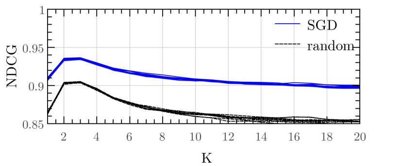
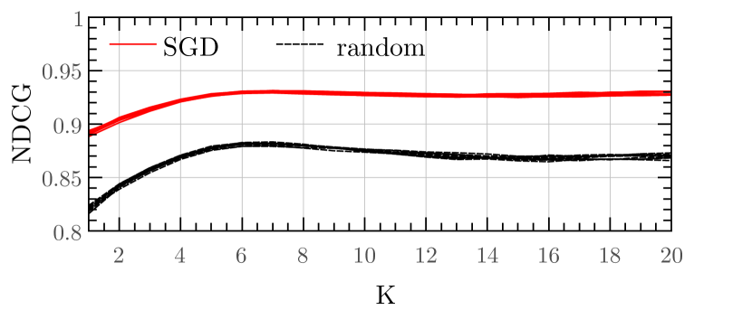
As indicated in Table 1, bottom, and in Fig. 5, the scores have a peaked distribution. This indicates first that the rating prediction task makes less sense with these datasets. We trained up an SGD recommender by using 50% of the datasets and computed NDCG(k) for $K=1\dots 20$. To understand the performance of the model, we also measured the performance of a random recommender that predicts ratings uniform randomly. We repeated our experiments 10 times with 10 different random training and test sets. Fig. 9 shows the computed ten performance curves for the SGD and the baseline random recommendation. Both for SGD and the random prediction the ten curves are similar. This indicates the stability of our algorithms and evaluation metrics. We achieved significantly better result with the SGD recommender. However for the random algorithm, the baseline NDCG is around 0.85. This is due to the fact that most of the ratings are around the mean as the score distribution is peaked.

Figure 9: Performance of score prediction on the France (top) and Paris (bottom) datasets.

5.3 Improving top recommendation with rating imputation

Instead of simply recommending locations near to already visited places, we expand the training set by relying on the locality of the ratings. We compare our results by using SVD or SGD both for the rating matrix and for simply predicting the visits, i.e. the existence of a rating regardless of its value. When considering locality, we may identify the nearest neighbors by taking the absolute distance and possibly correcting by density: in an area densely served by POIs, customers may reach more locations, on the other hand, the speed of travel is likely lower than in rural areas.

For our imputation methods, let $E$ be the set of known ratings and $N_{j}$ the neighbors of location $j$. We modify the training set as follows. For all $(u,i)$,

where $f$ is function of $R_{u}$, the set of known ratings by user $u$, and $N_{u,i}$, the set locations visited by $u$ in the neighborhood of $i$.

In our model, we expand the list of locations per user with the neighbors of visited places by the two strategies:

Constant:

$$f(R_{u},N_{u,i})=c$$ (16)

Ratings Average:

$$f(R_{u},N_{u,i})=\frac{1}{|N_{u,i}|}\sum_{j\in N_{u,i}}r_{u,j}$$ (17)

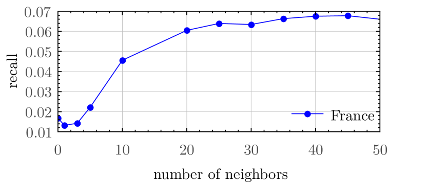
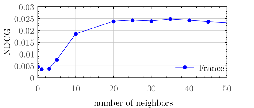
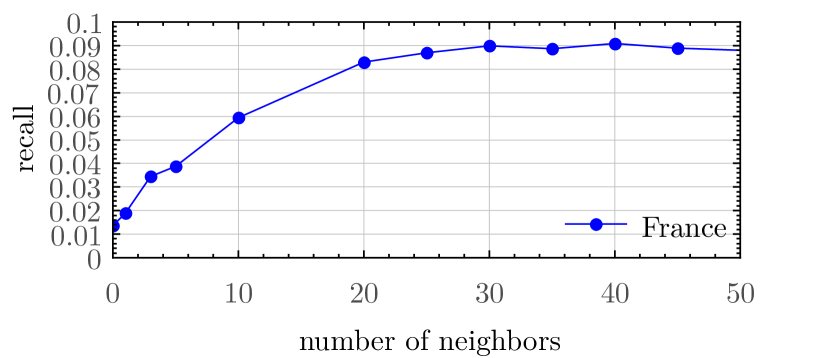
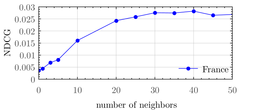
The performance for expansion with the original ratings (see (17)) on the France dataset is seen in Fig. 10 where we observe that expansion by the 30-40 nearest POIs improves significantly the matrix approximation by the first few eigenvectors.

We may also consider the task of predicting which POIs the user will visit, regardless of the actual rating given by the user. In this so-called implicit recommendation task, we consider a 0–1 matrix. Although the matrix is fully known, the meaning of a “1” is certain while a “0” may simply mean that the user has not yet had a chance to visit the POI or does not even know about it. Based on (16), the performance of the implicit task with expansion for the France dataset is seen in Fig. 11 showing an improvement compared to Fig. 10. However, for the Paris dataset, both in case of the ratings and implicit expansion experiments, we could not improve further the original SVD. This can be due to the fact that the Paris dataset is more dense geographically.

Figure 10: Recall@100 and NDCG@100 for expansion with the original ratings.

Figure 11: Recall@100 and NDCG@100 for expansion nearby visited locations.

5.4 Improving recommendation with fixed factors

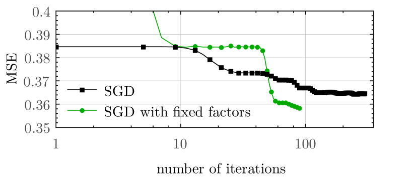
Results of Fig. 7 indicate that while SGD finds the most important cities in France, it can not separate them precisely. Furthermore, not recommending to a user POIs, that he/she have not visited, can be easily implemented without using SGD. Indeed, SGD should learn the taste of the different users like in case of the movie prediction task of Netflix. To fix this issue in the France dataset, we selected the top $t$ cities in France. For a given item, we fixed the first $i$th factor to 1, if the item is located in the $i$th city, and 0 otherwise. We set the user factors similarly according to the places visited by the user in the test set. We then trained a $k$ dimensional latent factor model where we updated only the remaining $k-t$ dimensions. We compared this recommender with a traditional $k$ dimensional SGD recommender.

In our experiments we included the top $t=10$ cities, in order Paris, Marseille, Lyon, Toulouse, Nice, Nantes, Strasbourg, Montpellier, Bordeaux, and Lille. Fig. 12 shows the MSE on the test set as the function of the number of iterations on the training set. With the fixed factor model we can achieve significantly better MSE. Furthermore, our best result is achieved with half less iterations compared to the number needed to train the original latent factor model.

Figure 12: Improved MSE results with fixed factors on the France dataset.

6 Discussion

Our statistical analysis of NOMAO votes of customers for spots of France shows that it is described by a power law frequency distributions with exponents $a\approx 1.5$ (for spots) and $b\approx 2.75$ (for customers) which remain stable in time even is the number of votes is increased almost by two orders of magnitude during this time period. Further studies are required to establish the physical origins of such laws and to clarify for universal they are. It is possible that the physical reasons for emergence of such type distributions have certain similarities with the phenomenon of self-organized criticality broadly discussed in physical systems (see e.g. bak ; wikiabelsand ; wikiselfcrit ). It is interesting to note that the exponent of cluster distribution in self-organized critical models in 3D has an exponent close to $1.4$ bak being not so far from the exponent $a=1.5$ we find for spots.

We explored the spectrum and the singular vectors of a POI ratings matrix of customer votes for spots of France. The fact that the matrix consists of 99.5% missing values makes the spectrum highly dependent on how we handle the missing values. We computed the SVD of the full 0–1 “implicit” matrix of the visits without considering the rating. For the ratings matrix, we used SGD, a popular approach that uses only the known values to compute the factors. We observed that SGD and SVD factors are similar but SVD has stronger geo-localization. SVD singular vectors with highest eigenvalues are mostly correlated with a particular place. As key practical observations, we found that imputing the missing ratings for the neighbors of visited places could increase the performance, and that defining fixed Geographic factors could improve SGD recommendation quality.

We expect that a broader analysis of a larger number of similar type datasets of votes will allow to gain better understanding of underlying physical process and provide better recommendations for specific customers and spots.

7 Acknowledgments

We thank the representatives of NOMAO nomaocom and especially Estelle Delpech (NOMAO) for providing us with the friendly access to the NOMAO datasets. This research is supported in part by the EC FET Open project “New tools and algorithms for directed network analysis” (NADINE $No$ 288956).

References

- (1) P. Bak, C. Tang and K. Wiesenfeld, Self-organized criticality: an explanation of 1/f noise, Phys. Rev. Lett. 59(4), 381 (1987)
- (2) J. Bao, Y. Zheng, D. Wilkie, and M. F. Mokbel, A survey on recommendations in location-based social networks. ACM Transaction on Intelligent Systems and Technology (to be published) (2013)
- (3) R. M. Bell and Y. Koren, Lessons from the Netflix prize challenge. ACM SIGKDD Explorations Newsletter 9(2), 75 (2007)
- (4) J. Bennett and S. Lanning, The Netflix prize, KDD Cup and Workshop in conjunction with KDD 2007, (2007).
- (5) D. Billsus and M. J. Pazzani, Learning collaborative information filters. ICML ’98: Proceedings of the Fifteenth International Conference on Machine Learning, pages 46–54, San Francisco, CA, USA, Morgan Kaufmann Publishers Inc. (1998)
- (6) J. Canny, Collaborative filtering with privacy via factor analysis, SIGIR ’02: Proceedings of the 25th annual international ACM SIGIR conference on Research and development in information retrieval, p.238, New York, NY, USA, ACM Press (2002)
- (7) C. Cheng, H. Yang, I. King, and M. R. Lyu, Fused matrix factorization with geographical and social influence in location-based social networks, AAAI 12, 1 (2012).
- (8) P. Cremonesi, Y. Koren, and R. Turrin, Performance of recommender algorithms on top-n recommendation tasks, Proceedings of the fourth ACM conference on Recommender systems, ACM p.39 (2010).
- (9) M. Deshpande and G. Karypis, Item-based top-n recommendation algorithms, ACM Transactions on Information Systems (TOIS) 22(1), 143 (2004).
- (10) S. Dorogovtsev, Lectures on complex networks, Oxford University Press, Oxford (2010)
- (11) J. H. Friedman, Greedy function approximation: A gradient boosting machine, The Annals of Statistics 29(5), 1189 (2001)
- (12) S. Funk, Netflix update: Try this at home, http://sifter.org/~simon/journal/20061211.html, 2006.
- (13) K. R. Gabriel and S. Zamir, Lower rank approximation of matrices by least squares with any choice of weights, Technometrics 21, 489 (1979)
- (14) G. H. Golub and C. F. V. Loan, Matrix Computations. Johns Hopkins University Press, Baltimore (1983)
- (15) D. Gupta, M. Digiovanni, H. Narita, and K. Goldberg, Jester 2.0 (poster abstract): evaluation of an new linear time collaborative filtering algorithm, SIGIR ’99: Proceedings of the 22nd annual international ACM SIGIR conference on Research and development in information retrieval, p.291, ACM Press, New York, NY, USA (1999)
- (16) Y. Koren, R. Bell, and C. Volinsky, Matrix factorization techniques for recommender systems, Computer 42(8), 30 (2009)
- (17) T. Kurashima, T. Iwata, G. Irie, and K. Fujimura, Travel route recommendation using geotags in photo sharing sites, Proceedings of the 19th ACM international conference on Information and knowledge management, ACM p.579 (2010)
- (18) M. Kurucz, A. A. Benczúr, K. Csalogány, and L. Lukács, Spectral clustering in telephone call graphs WebKDD/SNAKDD Workshop 2007 in conjunction with KDD 2007, (2007)
- (19) J. J. Levandoski, M. Sarwat, A. Eldawy, and M. F. Mokbel, Lars: A location-aware recommender system, Data Engineering (ICDE), 2012 IEEE 28th International Conference on, IEEE p.450 (2012)
- (20) NOMAO company, official web site http://fr.nomao.com/ . Web. 26 Apr. 2015
- (21) M. H. Pryor, The effects of singular value decomposition on collaborative filtering, Technical report, Dartmouth College, Hanover, NH, USA (1998)
- (22) B. Sarwar, G. Karypis, J. Konstan, and J. Riedl, Application of dimensionality reduction in recommender systems–a case study, ACM WebKDD Workshop (2000)
- (23) N. Srebro and T. Jaakkola, Weighted low-rank approximations, T. Fawcett and N. Mishra, editors, ICML, AAAI Press p.720 (2003)
- (24) P. Symeonidis, D. Ntempos, and Y. Manolopoulos, Location-based social networks, Recommender Systems for Location-based Social Networks, Springer, Berlin, p.35 (2014)
- (25) G. Takács, I. Pilászy, B. Németh, and D. Tikk, Investigation of various matrix factorization methods for large recommender systems. Proceedings of the 2nd KDD Workshop on Large-Scale Recommender Systems and the Netflix Prize Competition, ACM p.1 (2008)
- (26) G. Takács, I. Pilászy, B. Németh, and D. Tikk, A unified approach of factor models and neighbor based methods for large recommender systems, Applications of Digital Information and Web Technologies, 2008, ICADIWT 2008, First International Conference IEEE p.186 (2008)
- (27) Wikipedia contributors, Abelian sandpile model, Wikipedia, The Free Encyclopedia. Wikipedia, The Free Encyclopedia, 8 Apr. 2015, Web. 26 Apr. (2015)
- (28) Wikipedia contributors, Netflix Prize, Wikipedia, The Free Encyclopedia. Wikipedia, The Free Encyclopedia, 11 Feb. 2015, Web. 26 Apr. (2015)
- (29) Wikipedia contributors, Recommender system, Wikipedia, The Free Encyclopedia. Wikipedia, The Free Encyclopedia, 1 Apr. 2015, Web. 26 Apr. (2015)
- (30) Wikipedia contributors, Self-organized criticality , Wikipedia, The Free Encyclopedia. Wikipedia, The Free Encyclopedia, 13 Apr. 2015, Web. 28 Apr. (2015)
- (31) M. Ye, P. Yin, and W.-C. Lee, Location recommendation for location-based social networks, Proceedings of the 18th SIGSPATIAL International Conference on Advances in Geographic Information Systems, ACM p.458 (2010)
- (32) M. Ye, P. Yin, W.-C. Lee, and D.-L. Lee, Exploiting geographical influence for collaborative point-of-interest recommendation, Proceedings of the 34th international ACM SIGIR conference on Research and development in Information Retrieval, ACM p.325 (2011)
- (33) Q. Yuan, L. Chen, and S. Zhao, Factorization vs. regularization: fusing heterogeneous social relationships in top-n recommendation, Proceedings of the fifth ACM conference on Recommender systems, ACM p.245 (2011)
- (34) S. Zhang, W. Wang, J. Ford, F. Makedon, and J. Pearlman, Using singular value decomposition approximation for collaborative filtering, CEC ’05: Proceedings of the Seventh IEEE International Conference on E-Commerce Technology (CEC’05), Washington, DC, USA, IEEE Computer Society p.257 (2005)