Optimal Data and Training Symbol Ratio for Communication over Uncertain Channels

Ather Gattami Ericsson Research
Stockholm, Sweden
Email: ather.gattami@ericsson.com
Abstract

We consider the problem of determining the power ratio between the training symbols and data symbols in order to maximize the channel capacity for transmission over uncertain channels with a channel estimate available at both the transmitter and receiver. The receiver makes an estimate of the channel by using a known sequence of training symbols. This channel estimate is then transmitted back to the transmitter. The capacity that the transceiver maximizes is the worst case capacity, in the sense that given a noise covariance, the transceiver maximizes the minimal capacity over all distributions of the measurement noise under a fixed covariance matrix known at both the transmitter and receiver. We give an exact expression of the channel capacity as a function of the channel covariance matrix, and the number of training symbols used during a coherence time interval. This expression determines the number of training symbols that need to be used by finding the optimal integer number of training symbols that maximize the channel capacity. As a bi-product, we show that linear filters are optimal at both the transmitter and receiver.

Notation

det(A)๐ด\det(A) det(A)=โˆiฮปi๐ดsubscriptproduct๐‘–subscript๐œ†๐‘–\det(A)=\prod_{i}\lambda_{i}, where {ฮปi}subscript๐œ†๐‘–\{\lambda_{i}\}
are the eigenvalues of the square matrix A๐ดA.
โŠ—tensor-product\otimes AโŠ—Btensor-product๐ด๐ตA\otimes B denotes the kronecker product between
the matrices A๐ดA and B๐ตB.
๐„โ€‹{โ‹…}๐„โ‹…\mathbf{E}\{\cdot\} ๐„โ€‹{x}๐„๐‘ฅ\mathbf{E}\{x\} denotes the expected value of the
stochastic variable x๐‘ฅx.
๐„{โ‹…|โ‹…}\mathbf{E}\{\cdot|\cdot\} ๐„โ€‹{x|y}๐„conditional-set๐‘ฅ๐‘ฆ\mathbf{E}\{x|y\} denotes the expected value of the
stochastic variable x๐‘ฅx given y๐‘ฆy.
๐œ๐จ๐ฏ๐œ๐จ๐ฏ\mathbf{cov} ๐œ๐จ๐ฏโ€‹{x,y}=๐„โ€‹{xโ€‹yโˆ—}๐œ๐จ๐ฏ๐‘ฅ๐‘ฆ๐„๐‘ฅsuperscript๐‘ฆ\mathbf{cov}\{x,y\}={\mathbf{E}}\left\{xy^{*}\right\}.
hโ€‹(x)โ„Ž๐‘ฅh(x) Denotes the entropy of x๐‘ฅx.
hโ€‹(x|y)โ„Žconditional๐‘ฅ๐‘ฆh(x|y) Denotes the entropy of x๐‘ฅx given y๐‘ฆy.
Iโ€‹(x;y)I๐‘ฅ๐‘ฆ\textup{I}(x;y) Denotes the mutual information between
x๐‘ฅx and y๐‘ฆy.
๐’ฉโ€‹(m,V)๐’ฉ๐‘š๐‘‰\mathcal{N}(m,V) Denotes the set of Gaussian variables with
mean m๐‘šm and covariance V๐‘‰V.

I Introduction

I-A Background

This work considers the problem of determining the power ratio between the training symbols and data symbols in order to maximize the channel capacity for transmission over uncertain channels with channel state information at the transmitter and receiver. While the problem of MIMO communication over a channel known at the transmitter and receiver is well understood, the problem of uncertain channels still needs a deeper understanding of how much power we should spend on estimating the channel in order to transmit as much data as possible. This problem poses a trade-off between the power ratio allocated for training and data transmission. On one hand, if we spend more power on training and less on data transmission, the data throughput will be small of course. On the other hand, if we spend most of the power on data transmission and much less on training, the channel estimate will be bad and therefore, the channel estimation error noise will be large, causing a rather low data rate. Given per symbol power constraints, one might need a number of training symbols in order to achieve a certain quality of channel state information, which leaves a smaller number of symbols for data transmission. This is an important constraint that we take into account in this work.

I-B Previous Work

There has been a lot of work on MIMO communication in the context of uncertain channel state information. The seminal paper of Telatar [7] studied the problem of communication over uncertain Gaussian channels under the assumption that the channel realization is available at the receiver but not the transmitter. However, in practice, the transmitter and receiver donโ€™t have full knowledge of the channel. The work was extended in [6] for the case of slowly varying channels. The channel estimation extension of [7] was presented in [3], where the problem of power ratio between the training and data symbols was studied under average and per symbol power constraints over the channel coherence time(the time where the channel is roughly constant). The crucial assumption of average power constraint allows for spending only one symbol on training, since the power is only limited by the total power resource available during the coherence time. For the case of per symbol power constraints, the power ratio is harder to compute. The case where a channel estimate is available at the transmitter and reciever was studied in [1] under the specific signaling strategy of zero-forcing linear beamforming and given Gaussian measurement noise. Calculation of the channel capacity with respect to a channel estimate available at the receiver only was given in [2].

I-C Contribution

We consider communication over uncertain channels with channel state feedback at the transmitter. The receiver makes an estimate of the channel by using a known sequence of training symbols. This channel estimate is then transmitted back to the transmitter. The capacity that the transceiver maximizes is the worst case capacity, in the sense that given a noise covariance, the transceiver maximizes the minimal capacity over all distributions of the measurement noise under a fixed covariance matrix known at both the transmitter and receiver. The channel estimation error implies that the covariance of the transmitted symbols over time affects both the covariance of the transmitted information symbols and the total noise covariance, which makes the signal structure more complicated, where itโ€™s not clear if the symbols should be uncorrelated over time. For the single input multiple output (SIMO) channel, we give an exact expression of the channel capacity as a function of the channel covariance matrix, the noise covariance matrix, and the number of training symbols used during a coherence time interval. This expression determines the number of training symbols that need to be used by finding the optimal integer number of training symbols that maximize the channel capacity. Numerical examples illustrate the trade-off between the number of training and data symbols. The results indicate that when the transmission power (or equivalently the signal to noise ratio) is high, a smaller number of training symbols is required to maximize the capacity compared to the low transmission power case. We confirm these observations theoretically considering the asymptotic behavior of the power as it grows large or decreases to very small values.

II Preliminaries

Definition 1 (Kronecker Product)

For two matrices Aโˆˆโ„mร—n๐ดsuperscriptโ„๐‘š๐‘›A\in\mathbb{R}^{m\times n} and Bโˆˆโ„pร—q๐ตsuperscriptโ„๐‘๐‘žB\in\mathbb{R}^{p\times q}, the Kronecker product is defined as

AโŠ—B=(a11โ€‹Ba12โ€‹Bโ‹ฏa1โ€‹nโ€‹Ba21โ€‹Ba22โ€‹Bโ‹ฏa2โ€‹nโ€‹Bโ‹ฎโ‹ฎโ‹ฑโ‹ฎamโ€‹1โ€‹Bamโ€‹2โ€‹Bโ‹ฏamโ€‹nโ€‹B)tensor-product๐ด๐ตmatrixsubscript๐‘Ž11๐ตsubscript๐‘Ž12๐ตโ‹ฏsubscript๐‘Ž1๐‘›๐ตsubscript๐‘Ž21๐ตsubscript๐‘Ž22๐ตโ‹ฏsubscript๐‘Ž2๐‘›๐ตโ‹ฎโ‹ฎโ‹ฑโ‹ฎsubscript๐‘Ž๐‘š1๐ตsubscript๐‘Ž๐‘š2๐ตโ‹ฏsubscript๐‘Ž๐‘š๐‘›๐ตA\otimes B=\begin{pmatrix}a_{11}B&a_{12}B&\cdots&a_{1n}B\\ a_{21}B&a_{22}B&\cdots&a_{2n}B\\ \vdots&\vdots&\ddots&\vdots\\ a_{m1}B&a_{m2}B&\cdots&a_{mn}B\end{pmatrix}
Proposition 1 (Mutliplication Property of the Kronecker Product)

For any set of matrices A,B,C,D๐ด๐ต๐ถ๐ทA,B,C,D, we have that

(AโŠ—B)โ€‹(CโŠ—D)=Aโ€‹CโŠ—Bโ€‹Dtensor-product๐ด๐ตtensor-product๐ถ๐ทtensor-product๐ด๐ถ๐ต๐ท(A\otimes B)(C\otimes D)=AC\otimes BD
Proof:

Consult [4]. โˆŽ

Proposition 2 (Determinant Property)

For any two matrices Aโˆˆโ„mร—n๐ดsuperscriptโ„๐‘š๐‘›A\in\mathbb{R}^{m\times n} and Bโˆˆโ„nร—m๐ตsuperscriptโ„๐‘›๐‘šB\in\mathbb{R}^{n\times m}, we have that

det(Aโ€‹B+Im)=det(Bโ€‹A+In)๐ด๐ตsubscript๐ผ๐‘š๐ต๐ดsubscript๐ผ๐‘›\det(AB+I_{m})=\det(BA+I_{n})
Proof:

Consult [5]. โˆŽ

Proposition 3 (AM-GM Inequality)

Let a1,a2,โ€ฆ,ansubscript๐‘Ž1subscript๐‘Ž2โ€ฆsubscript๐‘Ž๐‘›a_{1},a_{2},...,a_{n} be n๐‘›n nonnegative real numbers. Then

1nโ€‹โˆ‘i=1naiโ‰ฅโˆi=1nain1๐‘›superscriptsubscript๐‘–1๐‘›subscript๐‘Ž๐‘–๐‘›superscriptsubscriptproduct๐‘–1๐‘›subscript๐‘Ž๐‘–\frac{1}{n}\sum_{i=1}^{n}a_{i}\geq\sqrt[n]{\prod_{i=1}^{n}a_{i}}

with equality if and only if a1=a2=โ‹ฏ=ansubscript๐‘Ž1subscript๐‘Ž2โ‹ฏsubscript๐‘Ž๐‘›a_{1}=a_{2}=\cdots=a_{n}.

Proof:

The proof may be found in most standard textbooks on Calculus. โˆŽ

III Problem Formulation

Let H๐ปH be a random channel such that ๐ฏ๐ž๐œโ€‹(H)โˆผ๐’žโ€‹๐’ฉโ€‹(0,C)similar-to๐ฏ๐ž๐œ๐ป๐’ž๐’ฉ0๐ถ{\mathbf{vec}}\left(H\right)\sim{\mathcal{CN}}\left(0,C\right). The realization of the channel is assumed to be constant over a coherence time interval corresponding to a block of T๐‘‡T symbols. Let xโ€‹(t)โˆผ๐’žโ€‹๐’ฉโ€‹(0,X)similar-to๐‘ฅ๐‘ก๐’ž๐’ฉ0๐‘‹x(t)\sim{\mathcal{CN}}\left(0,X\right) be the transmitted symbol over the Gaussian channel at time t๐‘กt. The received signal at time t๐‘กt is given by

yโ€‹(t)=Hโ€‹xโ€‹(t)+wโ€‹(t)๐‘ฆ๐‘ก๐ป๐‘ฅ๐‘ก๐‘ค๐‘กy(t)=Hx(t)+w(t)

where {wโ€‹(t)}๐‘ค๐‘ก\{w(t)\} is random white noise process, independent of H๐ปH and x๐‘ฅx, with zero mean and covariance given by ๐„โ€‹{wโ€‹(t)โ€‹wโˆ—โ€‹(t)}=Im๐„๐‘ค๐‘กsuperscript๐‘ค๐‘กsubscript๐ผ๐‘š{\mathbf{E}}\left\{w(t)w^{*}(t)\right\}=I_{m} known at both the transmitter and receiver. Without loss of generality, we assume that W๐‘ŠW is invertible.

Let (xโ€‹(1),โ€ฆ,xโ€‹(T))๐‘ฅ1โ€ฆ๐‘ฅ๐‘‡(x(1),...,x(T)) be the block symbols transmitted within the channel coherence time T๐‘‡T. The average power constraint imposed on the block is given by

1Tโ€‹โˆ‘t=1T๐„โ€‹{|xโ€‹(t)|2}โ‰คP1๐‘‡superscriptsubscript๐‘ก1๐‘‡๐„superscript๐‘ฅ๐‘ก2๐‘ƒ\frac{1}{T}\sum_{t=1}^{T}{\mathbf{E}}\left\{|x(t)|^{2}\right\}\leq P

The power constraint above could allow for some symbols xโ€‹(t)๐‘ฅ๐‘กx(t) to have a larger power than P๐‘ƒP. However, in the real world, we have hard constraints on the peak average power per symbol, so we will impose power constraints per symbol given by

๐„โ€‹{|xโ€‹(t)|2}โ‰คP,forย โ€‹t=1,โ€ฆ,Tformulae-sequence๐„superscript๐‘ฅ๐‘ก2๐‘ƒforย ๐‘ก1โ€ฆ๐‘‡{\mathbf{E}}\left\{|x(t)|^{2}\right\}\leq P,~{}~{}~{}~{}\text{for }~{}t=1,...,T

Suppose that we allocate Tฯ„subscript๐‘‡๐œT_{\tau} training symbols for the channel estimation part and Td=Tโˆ’Tฯ„subscript๐‘‡๐‘‘๐‘‡subscript๐‘‡๐œT_{d}=T-T_{\tau} symbols for data transmission. If a performance criterion is measured over the total channel coherence time T๐‘‡T, then clearly the optimal strategy is to transmit the training symbol sequence first followed by the data symbols. Also, when no energy constraints are present, the optimal power allocation is for each symbol to be transmitted with full power P๐‘ƒP. However, itโ€™s not clear what the optimal ratio between the training and data symbols. That is, what is the optimal choice of Tฯ„subscript๐‘‡๐œT_{\tau} to maximize the channel capacity? To this end, we will derive the exact expression of the channel capacity SIMO channel.

III-A SIMO Channel Estimation

Consider a random Gaussian channel H๐ปH taking values in โ„msuperscriptโ„๐‘š\mathbb{R}^{m}. Let xฯ„subscript๐‘ฅ๐œx_{\tau} be a deterministic training symbol known at the transmitter and receiver with |xฯ„|2=Psuperscriptsubscript๐‘ฅ๐œ2๐‘ƒ|x_{\tau}|^{2}=P. The transmitted training sequence is given by

xโ€‹(t)=xฯ„,forย โ€‹t=1,โ€ฆ,Tฯ„formulae-sequence๐‘ฅ๐‘กsubscript๐‘ฅ๐œforย ๐‘ก1โ€ฆsubscript๐‘‡๐œx(t)=x_{\tau},~{}~{}~{}~{}\text{for }~{}t=1,...,T_{\tau}

At the receiver, we obtain the measurement symbols

yโ€‹(t)=Hโ€‹xฯ„+wโ€‹(t),forย โ€‹t=1,โ€ฆ,Tฯ„formulae-sequence๐‘ฆ๐‘ก๐ปsubscript๐‘ฅ๐œ๐‘ค๐‘กforย ๐‘ก1โ€ฆsubscript๐‘‡๐œy(t)=Hx_{\tau}+w(t),~{}~{}~{}~{}\text{for }~{}t=1,...,T_{\tau}

Introduce the vectors

yฯ„=(yโ€‹(1)yโ€‹(2)โ‹ฎyโ€‹(Tฯ„)),wฯ„=(wโ€‹(1)wโ€‹(2)โ‹ฎwโ€‹(Tฯ„))formulae-sequencesubscript๐‘ฆ๐œmatrix๐‘ฆ1๐‘ฆ2โ‹ฎ๐‘ฆsubscript๐‘‡๐œsubscript๐‘ค๐œmatrix๐‘ค1๐‘ค2โ‹ฎ๐‘คsubscript๐‘‡๐œy_{\tau}=\begin{pmatrix}y(1)\\ y(2)\\ \vdots\\ y(T_{\tau})\end{pmatrix},~{}~{}~{}~{}w_{\tau}=\begin{pmatrix}w(1)\\ w(2)\\ \vdots\\ w(T_{\tau})\end{pmatrix}

and let the covariance matrix of wฯ„subscript๐‘ค๐œw_{\tau} be

๐„โ€‹{wฯ„โ€‹wฯ„โˆ—}=ImโŠ—ITฯ„=Imโ€‹Tฯ„๐„subscript๐‘ค๐œsuperscriptsubscript๐‘ค๐œtensor-productsubscript๐ผ๐‘šsubscript๐ผsubscript๐‘‡๐œsubscript๐ผ๐‘šsubscript๐‘‡๐œ{\mathbf{E}}\left\{w_{\tau}w_{\tau}^{*}\right\}=I_{m}\otimes I_{T_{\tau}}=I_{mT_{\tau}}

Itโ€™s well known that the optimal estimator H^^๐ป\hat{H} of H๐ปH given yฯ„subscript๐‘ฆ๐œy_{\tau} that minimizes the MSE is given by

H^^๐ป\displaystyle\hat{H} =๐„โ€‹{H|yฯ„}absent๐„conditional-set๐ปsubscript๐‘ฆ๐œ\displaystyle={\mathbf{E}}\left\{H~{}|~{}y_{\tau}\right\} (1)
=๐œ๐จ๐ฏโ€‹(H,yฯ„)โ‹…๐œ๐จ๐ฏโ€‹(yฯ„,yฯ„)โˆ’1โ€‹yฯ„absentโ‹…๐œ๐จ๐ฏ๐ปsubscript๐‘ฆ๐œ๐œ๐จ๐ฏsuperscriptsubscript๐‘ฆ๐œsubscript๐‘ฆ๐œ1subscript๐‘ฆ๐œ\displaystyle={\mathbf{cov}}\left(H,y_{\tau}\right)\cdot{\mathbf{cov}}\left(y_{\tau},y_{\tau}\right)^{-1}y_{\tau} (2)
=๐„โ€‹{Hโ€‹yฯ„โˆ—}โ‹…๐„โ€‹{yฯ„โ€‹yฯ„โˆ—}โˆ’1โ€‹yฯ„absentโ‹…๐„๐ปsubscriptsuperscript๐‘ฆ๐œ๐„superscriptsubscript๐‘ฆ๐œsuperscriptsubscript๐‘ฆ๐œ1subscript๐‘ฆ๐œ\displaystyle={\mathbf{E}}\left\{Hy^{*}_{\tau}\right\}\cdot{\mathbf{E}}\left\{y_{\tau}y_{\tau}^{*}\right\}^{-1}y_{\tau} (3)
=xฯ„โˆ—โ€‹Cโ€‹(Pโ€‹C+1Tฯ„โ€‹Im)โˆ’1โ€‹1Tฯ„โ€‹โˆ‘t=1Tฯ„yโ€‹(t)absentsubscriptsuperscript๐‘ฅ๐œ๐ถsuperscript๐‘ƒ๐ถ1subscript๐‘‡๐œsubscript๐ผ๐‘š11subscript๐‘‡๐œsuperscriptsubscript๐‘ก1subscript๐‘‡๐œ๐‘ฆ๐‘ก\displaystyle=x^{*}_{\tau}C\left(PC+\frac{1}{T_{\tau}}I_{m}\right)^{-1}\frac{1}{T_{\tau}}\sum_{t=1}^{T_{\tau}}y(t) (4)
=xฯ„โˆ—โ€‹Cโ€‹(Pโ€‹C+1Tฯ„โ€‹Im)โˆ’1โ€‹(Hโ€‹xฯ„+wยฏโ€‹(t))absentsubscriptsuperscript๐‘ฅ๐œ๐ถsuperscript๐‘ƒ๐ถ1subscript๐‘‡๐œsubscript๐ผ๐‘š1๐ปsubscript๐‘ฅ๐œยฏ๐‘ค๐‘ก\displaystyle=x^{*}_{\tau}C\left(PC+\frac{1}{T_{\tau}}I_{m}\right)^{-1}(Hx_{\tau}+\bar{w}(t)) (5)

where

wยฏโ€‹(t)=1Tฯ„โ€‹โˆ‘t=1Tฯ„wโ€‹(t)ยฏ๐‘ค๐‘ก1subscript๐‘‡๐œsuperscriptsubscript๐‘ก1subscript๐‘‡๐œ๐‘ค๐‘ก\bar{w}(t)=\frac{1}{T_{\tau}}\sum_{t=1}^{T_{\tau}}w(t)

The covariance of wยฏโ€‹(t)ยฏ๐‘ค๐‘ก\bar{w}(t) is easily obtained from the expression above, and itโ€™s given by

๐„โ€‹{wยฏโ€‹(t)โ€‹wยฏโˆ—โ€‹(t)}=1Tฯ„โ€‹Im๐„ยฏ๐‘ค๐‘กsuperscriptยฏ๐‘ค๐‘ก1subscript๐‘‡๐œsubscript๐ผ๐‘š{\mathbf{E}}\left\{\bar{w}(t)\bar{w}^{*}(t)\right\}=\frac{1}{T_{\tau}}I_{m}

The channel estimation error is given by

H~~๐ป\displaystyle\tilde{H} =Hโˆ’H^absent๐ป^๐ป\displaystyle=H-\hat{H} (6)
=Hโˆ’xฯ„โˆ—โ€‹Cโ€‹(Pโ€‹C+1Tฯ„โ€‹Im)โˆ’1โ€‹(Hโ€‹xฯ„+wยฏโ€‹(t))absent๐ปsubscriptsuperscript๐‘ฅ๐œ๐ถsuperscript๐‘ƒ๐ถ1subscript๐‘‡๐œsubscript๐ผ๐‘š1๐ปsubscript๐‘ฅ๐œยฏ๐‘ค๐‘ก\displaystyle=H-x^{*}_{\tau}C\left(PC+\frac{1}{T_{\tau}}I_{m}\right)^{-1}(Hx_{\tau}+\bar{w}(t)) (7)
=(Imโˆ’Pโ€‹Cโ€‹(Pโ€‹C+1Tฯ„โ€‹Im)โˆ’1)โ€‹Habsentsubscript๐ผ๐‘š๐‘ƒ๐ถsuperscript๐‘ƒ๐ถ1subscript๐‘‡๐œsubscript๐ผ๐‘š1๐ป\displaystyle=(I_{m}-PC\left(PC+\frac{1}{T_{\tau}}I_{m}\right)^{-1})H
โˆ’xฯ„โˆ—โ€‹Cโ€‹(Pโ€‹C+1Tฯ„โ€‹Im)โˆ’1โ€‹wยฏโ€‹(t)subscriptsuperscript๐‘ฅ๐œ๐ถsuperscript๐‘ƒ๐ถ1subscript๐‘‡๐œsubscript๐ผ๐‘š1ยฏ๐‘ค๐‘ก\displaystyle~{}~{}~{}-x^{*}_{\tau}C\left(PC+\frac{1}{T_{\tau}}I_{m}\right)^{-1}\bar{w}(t) (8)
=1Tฯ„โ€‹(Pโ€‹C+1Tฯ„โ€‹Im)โˆ’1โ€‹Habsent1subscript๐‘‡๐œsuperscript๐‘ƒ๐ถ1subscript๐‘‡๐œsubscript๐ผ๐‘š1๐ป\displaystyle=\frac{1}{T_{\tau}}\left(PC+\frac{1}{T_{\tau}}I_{m}\right)^{-1}H
โˆ’xฯ„โˆ—โ€‹Cโ€‹(Pโ€‹C+1Tฯ„โ€‹Im)โˆ’1โ€‹wยฏโ€‹(t)subscriptsuperscript๐‘ฅ๐œ๐ถsuperscript๐‘ƒ๐ถ1subscript๐‘‡๐œsubscript๐ผ๐‘š1ยฏ๐‘ค๐‘ก\displaystyle~{}~{}~{}-x^{*}_{\tau}C\left(PC+\frac{1}{T_{\tau}}I_{m}\right)^{-1}\bar{w}(t) (9)

Now we have that

C^^๐ถ\displaystyle\hat{C} =๐„โ€‹{C^}absent๐„^๐ถ\displaystyle={\mathbf{E}}\left\{\hat{C}\right\} (10)
=Pโ€‹Cโ€‹(Pโ€‹C+1Tฯ„โ€‹Im)โˆ’1โ€‹Cabsent๐‘ƒ๐ถsuperscript๐‘ƒ๐ถ1subscript๐‘‡๐œsubscript๐ผ๐‘š1๐ถ\displaystyle=PC\left(PC+\frac{1}{T_{\tau}}I_{m}\right)^{-1}C (11)

Itโ€™s well known that H^^๐ป\hat{H} and H~~๐ป\tilde{H} are independent since H๐ปH and yฯ„subscript๐‘ฆ๐œy_{\tau} are jointly Gaussian. Thus,

C~~๐ถ\displaystyle\tilde{C} =๐„โ€‹{H~โ€‹H~โˆ—}absent๐„~๐ปsuperscript~๐ป\displaystyle={\mathbf{E}}\left\{\tilde{H}\tilde{H}^{*}\right\} (12)
=๐„โ€‹{(Hโˆ’H^)โ€‹(Hโˆ’H^)โˆ—}absent๐„๐ป^๐ปsuperscript๐ป^๐ป\displaystyle={\mathbf{E}}\left\{(H-\hat{H})(H-\hat{H})^{*}\right\} (13)
=Cโˆ’C^absent๐ถ^๐ถ\displaystyle=C-\hat{C} (14)
=Cโˆ’Pโ€‹Cโ€‹(Pโ€‹C+1Tฯ„โ€‹Im)โˆ’1โ€‹Cabsent๐ถ๐‘ƒ๐ถsuperscript๐‘ƒ๐ถ1subscript๐‘‡๐œsubscript๐ผ๐‘š1๐ถ\displaystyle=C-PC\left(PC+\frac{1}{T_{\tau}}I_{m}\right)^{-1}C (15)
=(Imโˆ’Pโ€‹Cโ€‹(Pโ€‹C+1Tฯ„โ€‹Im)โˆ’1)โ€‹Cabsentsubscript๐ผ๐‘š๐‘ƒ๐ถsuperscript๐‘ƒ๐ถ1subscript๐‘‡๐œsubscript๐ผ๐‘š1๐ถ\displaystyle=(I_{m}-PC\left(PC+\frac{1}{T_{\tau}}I_{m}\right)^{-1})C (16)
=1Tฯ„โ€‹(Pโ€‹C+1Tฯ„โ€‹Im)โˆ’1โ€‹Cabsent1subscript๐‘‡๐œsuperscript๐‘ƒ๐ถ1subscript๐‘‡๐œsubscript๐ผ๐‘š1๐ถ\displaystyle=\frac{1}{T_{\tau}}\left(PC+\frac{1}{T_{\tau}}I_{m}\right)^{-1}C (17)

III-B Channel Capacity

In this section, we will derive a formula for the channel capacity under the assumption that the transmitted and receiver have a common estimate of the channel. The estimate is the optimal estimate that minimizes the expected value of the variance of the estimation error.

Suppose that we transmit Tฯ„subscript๐‘‡๐œT_{\tau} training symbols during the time interval t=1,โ€ฆ,Tฯ„๐‘ก1โ€ฆsubscript๐‘‡๐œt=1,...,T_{\tau} and Td=Tโˆ’Tฯ„subscript๐‘‡๐‘‘๐‘‡subscript๐‘‡๐œT_{d}=T-T_{\tau} data symbols during the time interval t=Tฯ„+1,โ€ฆ,T๐‘กsubscript๐‘‡๐œ1โ€ฆ๐‘‡t=T_{\tau}+1,...,T. The received noisy measurements of the data symbols are given by

yโ€‹(t)๐‘ฆ๐‘ก\displaystyle y(t) =Hโ€‹xdโ€‹(t)+wโ€‹(t)absent๐ปsubscript๐‘ฅ๐‘‘๐‘ก๐‘ค๐‘ก\displaystyle=Hx_{d}(t)+w(t) (18)
=H^โ€‹xdโ€‹(t)+H~โ€‹xdโ€‹(t)+wโ€‹(t)absent^๐ปsubscript๐‘ฅ๐‘‘๐‘ก~๐ปsubscript๐‘ฅ๐‘‘๐‘ก๐‘ค๐‘ก\displaystyle=\hat{H}x_{d}(t)+\tilde{H}x_{d}(t)+w(t) (19)
=H^โ€‹xdโ€‹(t)+vโ€‹(t),absent^๐ปsubscript๐‘ฅ๐‘‘๐‘ก๐‘ฃ๐‘ก\displaystyle=\hat{H}x_{d}(t)+v(t), (20)

for t=Tฯ„+1,โ€ฆ,T๐‘กsubscript๐‘‡๐œ1โ€ฆ๐‘‡t=T_{\tau}+1,...,T. Note that vโ€‹(t)=H~โ€‹xdโ€‹(t)+wโ€‹(t)๐‘ฃ๐‘ก~๐ปsubscript๐‘ฅ๐‘‘๐‘ก๐‘ค๐‘กv(t)=\tilde{H}x_{d}(t)+w(t) is uncorrelated with xdโ€‹(t)subscript๐‘ฅ๐‘‘๐‘กx_{d}(t) and H^โ€‹xdโ€‹(t)^๐ปsubscript๐‘ฅ๐‘‘๐‘ก\hat{H}x_{d}(t) jointly. Introduce the vectors

yd=(yโ€‹(Tฯ„+1)yโ€‹(Tฯ„+2)โ‹ฎyโ€‹(T)),xd=(xdโ€‹(Tฯ„+1)xdโ€‹(Tฯ„+2)โ‹ฎxdโ€‹(T))formulae-sequencesubscript๐‘ฆ๐‘‘matrix๐‘ฆsubscript๐‘‡๐œ1๐‘ฆsubscript๐‘‡๐œ2โ‹ฎ๐‘ฆ๐‘‡subscript๐‘ฅ๐‘‘matrixsubscript๐‘ฅ๐‘‘subscript๐‘‡๐œ1subscript๐‘ฅ๐‘‘subscript๐‘‡๐œ2โ‹ฎsubscript๐‘ฅ๐‘‘๐‘‡y_{d}=\begin{pmatrix}y(T_{\tau}+1)\\ y(T_{\tau}+2)\\ \vdots\\ y(T)\end{pmatrix},~{}~{}~{}~{}x_{d}=\begin{pmatrix}x_{d}(T_{\tau}+1)\\ x_{d}(T_{\tau}+2)\\ \vdots\\ x_{d}(T)\end{pmatrix}
wd=(wโ€‹(Tฯ„+1)wโ€‹(Tฯ„+2)โ‹ฎwโ€‹(T)),vd=(vโ€‹(Tฯ„+1)vโ€‹(Tฯ„+2)โ‹ฎvโ€‹(T))formulae-sequencesubscript๐‘ค๐‘‘matrix๐‘คsubscript๐‘‡๐œ1๐‘คsubscript๐‘‡๐œ2โ‹ฎ๐‘ค๐‘‡subscript๐‘ฃ๐‘‘matrix๐‘ฃsubscript๐‘‡๐œ1๐‘ฃsubscript๐‘‡๐œ2โ‹ฎ๐‘ฃ๐‘‡w_{d}=\begin{pmatrix}w(T_{\tau}+1)\\ w(T_{\tau}+2)\\ \vdots\\ w(T)\end{pmatrix},~{}~{}~{}~{}v_{d}=\begin{pmatrix}v(T_{\tau}+1)\\ v(T_{\tau}+2)\\ \vdots\\ v(T)\end{pmatrix}

and let the resepective covariance matrices of wdsubscript๐‘ค๐‘‘w_{d} and vdsubscript๐‘ฃ๐‘‘v_{d} be

Wd=๐„โ€‹{wdโ€‹wdโˆ—}=ImโŠ—ITd=Imโ€‹Tdsubscript๐‘Š๐‘‘๐„subscript๐‘ค๐‘‘superscriptsubscript๐‘ค๐‘‘tensor-productsubscript๐ผ๐‘šsubscript๐ผsubscript๐‘‡๐‘‘subscript๐ผ๐‘šsubscript๐‘‡๐‘‘W_{d}={\mathbf{E}}\left\{w_{d}w_{d}^{*}\right\}=I_{m}\otimes I_{T_{d}}=I_{mT_{d}}

and

Vd=๐„โ€‹{vdโ€‹vdโˆ—}=VโŠ—ITd=(V0โ‹ฏ00Vโ‹ฏ0โ‹ฎโ‹ฎโ‹ฑโ‹ฎ00โ‹ฏV)subscript๐‘‰๐‘‘๐„subscript๐‘ฃ๐‘‘superscriptsubscript๐‘ฃ๐‘‘tensor-product๐‘‰subscript๐ผsubscript๐‘‡๐‘‘matrix๐‘‰0โ‹ฏ00๐‘‰โ‹ฏ0โ‹ฎโ‹ฎโ‹ฑโ‹ฎ00โ‹ฏ๐‘‰V_{d}={\mathbf{E}}\left\{v_{d}v_{d}^{*}\right\}=V\otimes I_{T_{d}}=\begin{pmatrix}V&0&\cdots&0\\ 0&V&\cdots&0\\ \vdots&\vdots&\ddots&\vdots\\ 0&0&\cdots&V\end{pmatrix}

The worst case capacity of the channel with repsect to the measurement noise Imโ€‹Tdsubscript๐ผ๐‘šsubscript๐‘‡๐‘‘I_{mT_{d}} is given by

๐’žโ€‹(Tฯ„)=supxd๐„โ€‹{|xdโ€‹(t)|2}=Pinfvd๐„โ€‹{vdโ€‹vdโˆ—}=Imโ€‹TdIโ€‹(xd;yd)๐’žsubscript๐‘‡๐œsubscriptsupremumsubscript๐‘ฅ๐‘‘๐„superscriptsubscript๐‘ฅ๐‘‘๐‘ก2๐‘ƒsubscriptinfimumsubscript๐‘ฃ๐‘‘๐„subscript๐‘ฃ๐‘‘superscriptsubscript๐‘ฃ๐‘‘subscript๐ผ๐‘šsubscript๐‘‡๐‘‘Isubscript๐‘ฅ๐‘‘subscript๐‘ฆ๐‘‘\mathcal{C}(T_{\tau})=\sup_{\begin{subarray}{c}x_{d}\\ {\mathbf{E}}\left\{|x_{d}(t)|^{2}\right\}=P\end{subarray}}\inf_{\begin{subarray}{c}v_{d}\\ {\mathbf{E}}\left\{v_{d}v_{d}^{*}\right\}=I_{mT_{d}}\end{subarray}}\textup{I}(x_{d};y_{d}) (21)

Thus, the problem that we want to solve is as follows.

Problem 1

Find the optimal integer Tฯ„โˆˆ[1,T]subscript๐‘‡๐œ1๐‘‡T_{\tau}\in[1,T] such that

๐’žโ€‹(Tฯ„)=supxd๐„โ€‹{|xdโ€‹(t)|2}=Pinfvd๐„โ€‹{vdโ€‹vdโˆ—}=Imโ€‹TdIโ€‹(xd;yd)๐’žsubscript๐‘‡๐œsubscriptsupremumsubscript๐‘ฅ๐‘‘๐„superscriptsubscript๐‘ฅ๐‘‘๐‘ก2๐‘ƒsubscriptinfimumsubscript๐‘ฃ๐‘‘๐„subscript๐‘ฃ๐‘‘superscriptsubscript๐‘ฃ๐‘‘subscript๐ผ๐‘šsubscript๐‘‡๐‘‘Isubscript๐‘ฅ๐‘‘subscript๐‘ฆ๐‘‘\mathcal{C}(T_{\tau})=\sup_{\begin{subarray}{c}x_{d}\\ {\mathbf{E}}\left\{|x_{d}(t)|^{2}\right\}=P\end{subarray}}\inf_{\begin{subarray}{c}v_{d}\\ {\mathbf{E}}\left\{v_{d}v_{d}^{*}\right\}=I_{mT_{d}}\end{subarray}}\textup{I}(x_{d};y_{d})

is maximized.

IV Main Results

Itโ€™s well known that for a deterministic channel H^dsubscript^๐ป๐‘‘\hat{H}_{d} and signal measurement

yd=H^dโ€‹xd+vdsubscript๐‘ฆ๐‘‘subscript^๐ป๐‘‘subscript๐‘ฅ๐‘‘subscript๐‘ฃ๐‘‘y_{d}=\hat{H}_{d}x_{d}+v_{d}

with measurement noise vdsubscript๐‘ฃ๐‘‘v_{d} uncorrelated with the transmitted signal xdsubscript๐‘ฅ๐‘‘x_{d}, the optimal transmitting strategy is for xdsubscript๐‘ฅ๐‘‘x_{d} to be Gaussian in order to minimize the worst case noise vdsubscript๐‘ฃ๐‘‘v_{d} which is also shown to be Gaussian. In other words, the Gaussian input and noise form a Nash equilibrium. The case when the noise vdsubscript๐‘ฃ๐‘‘v_{d} has an arbitrary covariance matrix Vdsubscript๐‘‰๐‘‘V_{d} has been solved in [3]. In our case, the situation is different. The covariance matrix of vdsubscript๐‘ฃ๐‘‘v_{d} has a structure that also depends on the choice of the covariance matrix of the transmitted signal xdsubscript๐‘ฅ๐‘‘x_{d}. More precisely, recall that we have assumed that {wโ€‹(t)}๐‘ค๐‘ก\{w(t)\} is a temporally uncorrelated noise process with arbitrary distribution. Introduce

H^d=H^โŠ—ITd=(H^0โ‹ฏ00H^โ‹ฏ0โ‹ฎโ‹ฎโ‹ฑโ‹ฎ00โ‹ฏH^)subscript^๐ป๐‘‘tensor-product^๐ปsubscript๐ผsubscript๐‘‡๐‘‘matrix^๐ป0โ‹ฏ00^๐ปโ‹ฏ0โ‹ฎโ‹ฎโ‹ฑโ‹ฎ00โ‹ฏ^๐ป\hat{H}_{d}=\hat{H}\otimes I_{T_{d}}=\begin{pmatrix}\hat{H}&0&\cdots&0\\ 0&\hat{H}&\cdots&0\\ \vdots&\vdots&\ddots&\vdots\\ 0&0&\cdots&\hat{H}\end{pmatrix}

and

H~d=H~โŠ—ITd=(H~0โ‹ฏ00H~โ‹ฏ0โ‹ฎโ‹ฎโ‹ฑโ‹ฎ00โ‹ฏH~)subscript~๐ป๐‘‘tensor-product~๐ปsubscript๐ผsubscript๐‘‡๐‘‘matrix~๐ป0โ‹ฏ00~๐ปโ‹ฏ0โ‹ฎโ‹ฎโ‹ฑโ‹ฎ00โ‹ฏ~๐ป\tilde{H}_{d}=\tilde{H}\otimes I_{T_{d}}=\begin{pmatrix}\tilde{H}&0&\cdots&0\\ 0&\tilde{H}&\cdots&0\\ \vdots&\vdots&\ddots&\vdots\\ 0&0&\cdots&\tilde{H}\end{pmatrix}

We may write wd=vdโˆ’H~dโ€‹xdsubscript๐‘ค๐‘‘subscript๐‘ฃ๐‘‘subscript~๐ป๐‘‘subscript๐‘ฅ๐‘‘w_{d}=v_{d}-\tilde{H}_{d}x_{d}, with vdsubscript๐‘ฃ๐‘‘v_{d} uncorrelated with H^dsubscript^๐ป๐‘‘\hat{H}_{d} and xdsubscript๐‘ฅ๐‘‘x_{d}. Furthermore,

๐„โ€‹{vdโ€‹vdโˆ—}โˆ’๐„โ€‹{H~dโ€‹xdโ€‹xdโˆ—โ€‹H~dโˆ—}=๐„โ€‹{wdโ€‹wdโˆ—}=Imโ€‹Td๐„subscript๐‘ฃ๐‘‘superscriptsubscript๐‘ฃ๐‘‘๐„subscript~๐ป๐‘‘subscript๐‘ฅ๐‘‘superscriptsubscript๐‘ฅ๐‘‘superscriptsubscript~๐ป๐‘‘๐„subscript๐‘ค๐‘‘superscriptsubscript๐‘ค๐‘‘subscript๐ผ๐‘šsubscript๐‘‡๐‘‘{\mathbf{E}}\left\{v_{d}v_{d}^{*}\right\}-{\mathbf{E}}\left\{\tilde{H}_{d}x_{d}x_{d}^{*}\tilde{H}_{d}^{*}\right\}={\mathbf{E}}\left\{w_{d}w_{d}^{*}\right\}=I_{mT_{d}}

Let Xd=๐„โ€‹{xdโ€‹xdโˆ—}subscript๐‘‹๐‘‘๐„subscript๐‘ฅ๐‘‘superscriptsubscript๐‘ฅ๐‘‘X_{d}={\mathbf{E}}\left\{x_{d}x_{d}^{*}\right\}. Then we have

H^dโ€‹xd=(H^โ€‹xdโ€‹(Tฯ„+1)H^โ€‹xdโ€‹(Tฯ„+2)โ‹ฎH^โ€‹xdโ€‹(T))subscript^๐ป๐‘‘subscript๐‘ฅ๐‘‘matrix^๐ปsubscript๐‘ฅ๐‘‘subscript๐‘‡๐œ1^๐ปsubscript๐‘ฅ๐‘‘subscript๐‘‡๐œ2โ‹ฎ^๐ปsubscript๐‘ฅ๐‘‘๐‘‡\hat{H}_{d}x_{d}=\begin{pmatrix}\hat{H}x_{d}(T_{\tau}+1)\\ \hat{H}x_{d}(T_{\tau}+2)\\ \vdots\\ \hat{H}x_{d}(T)\end{pmatrix}

and the blocks of H^dโ€‹xdโ€‹xdโˆ—โ€‹H^dโˆ—subscript^๐ป๐‘‘subscript๐‘ฅ๐‘‘superscriptsubscript๐‘ฅ๐‘‘superscriptsubscript^๐ป๐‘‘\hat{H}_{d}x_{d}x_{d}^{*}\hat{H}_{d}^{*} at position (i,j)๐‘–๐‘—(i,j) will be given by(since xdโ€‹(Tฯ„+i)subscript๐‘ฅ๐‘‘subscript๐‘‡๐œ๐‘–x_{d}(T_{\tau}+i) is a scalar for all i=1,โ€ฆ,Tโˆ’Tฯ„๐‘–1โ€ฆ๐‘‡subscript๐‘‡๐œi=1,...,T-T_{\tau})

[H^dโ€‹xdโ€‹xdโˆ—โ€‹H^dโˆ—]iโ€‹jsubscriptdelimited-[]subscript^๐ป๐‘‘subscript๐‘ฅ๐‘‘superscriptsubscript๐‘ฅ๐‘‘superscriptsubscript^๐ป๐‘‘๐‘–๐‘—\displaystyle[\hat{H}_{d}x_{d}x_{d}^{*}\hat{H}_{d}^{*}]_{ij} =H^โ€‹xdโ€‹(Tฯ„+i)โ€‹xdโˆ—โ€‹(Tฯ„+j)โ€‹H^โˆ—absent^๐ปsubscript๐‘ฅ๐‘‘subscript๐‘‡๐œ๐‘–superscriptsubscript๐‘ฅ๐‘‘subscript๐‘‡๐œ๐‘—superscript^๐ป\displaystyle=\hat{H}x_{d}(T_{\tau}+i)x_{d}^{*}(T_{\tau}+j)\hat{H}^{*}
=xdโ€‹(Tฯ„+i)โ€‹xdโˆ—โ€‹(Tฯ„+j)โ€‹H^โ€‹H^โˆ—,absentsubscript๐‘ฅ๐‘‘subscript๐‘‡๐œ๐‘–superscriptsubscript๐‘ฅ๐‘‘subscript๐‘‡๐œ๐‘—^๐ปsuperscript^๐ป\displaystyle=x_{d}(T_{\tau}+i)x_{d}^{*}(T_{\tau}+j)\hat{H}\hat{H}^{*},

for i,j=1,โ€ฆ,Tโˆ’Tฯ„formulae-sequence๐‘–๐‘—1โ€ฆ๐‘‡subscript๐‘‡๐œi,j=1,...,T-T_{\tau}. Thus, H^dโ€‹xdโ€‹xdโˆ—โ€‹H^dโˆ—=(xdโ€‹xdโˆ—)โŠ—(H^โ€‹H^โˆ—)subscript^๐ป๐‘‘subscript๐‘ฅ๐‘‘superscriptsubscript๐‘ฅ๐‘‘superscriptsubscript^๐ป๐‘‘tensor-productsubscript๐‘ฅ๐‘‘superscriptsubscript๐‘ฅ๐‘‘^๐ปsuperscript^๐ป\hat{H}_{d}x_{d}x_{d}^{*}\hat{H}_{d}^{*}=(x_{d}x_{d}^{*})\otimes(\hat{H}\hat{H}^{*}) and given H^^๐ป\hat{H}, we get

๐„โ€‹{H~dโ€‹xdโ€‹xdโˆ—โ€‹H~dโˆ—}=XdโŠ—C^.๐„subscript~๐ป๐‘‘subscript๐‘ฅ๐‘‘superscriptsubscript๐‘ฅ๐‘‘superscriptsubscript~๐ป๐‘‘tensor-productsubscript๐‘‹๐‘‘^๐ถ{\mathbf{E}}\left\{\tilde{H}_{d}x_{d}x_{d}^{*}\tilde{H}_{d}^{*}\right\}=X_{d}\otimes\hat{C}.

Similarly, we get H~dโ€‹xdโ€‹xdโˆ—โ€‹H~dโˆ—=(xdโ€‹xdโˆ—)โŠ—(H~โ€‹H~โˆ—)subscript~๐ป๐‘‘subscript๐‘ฅ๐‘‘superscriptsubscript๐‘ฅ๐‘‘superscriptsubscript~๐ป๐‘‘tensor-productsubscript๐‘ฅ๐‘‘superscriptsubscript๐‘ฅ๐‘‘~๐ปsuperscript~๐ป\tilde{H}_{d}x_{d}x_{d}^{*}\tilde{H}_{d}^{*}=(x_{d}x_{d}^{*})\otimes(\tilde{H}\tilde{H}^{*}) and

๐„โ€‹{H~dโ€‹xdโ€‹xdโˆ—โ€‹H~dโˆ—}=XdโŠ—C~.๐„subscript~๐ป๐‘‘subscript๐‘ฅ๐‘‘superscriptsubscript๐‘ฅ๐‘‘superscriptsubscript~๐ป๐‘‘tensor-productsubscript๐‘‹๐‘‘~๐ถ{\mathbf{E}}\left\{\tilde{H}_{d}x_{d}x_{d}^{*}\tilde{H}_{d}^{*}\right\}=X_{d}\otimes\tilde{C}.

This gives in turn

Vd=๐„โ€‹{vdโ€‹vdโˆ—}=Imโ€‹Td+XdโŠ—C~subscript๐‘‰๐‘‘๐„subscript๐‘ฃ๐‘‘superscriptsubscript๐‘ฃ๐‘‘subscript๐ผ๐‘šsubscript๐‘‡๐‘‘tensor-productsubscript๐‘‹๐‘‘~๐ถV_{d}={\mathbf{E}}\left\{v_{d}v_{d}^{*}\right\}=I_{mT_{d}}+X_{d}\otimes\tilde{C}

In particular, the block diagonal elements of Vdsubscript๐‘‰๐‘‘V_{d} are equal, with the block elements given by

V=Im+๐„โ€‹{H~โ€‹Pโ€‹H~โˆ—}=Im+Pโ€‹C~๐‘‰subscript๐ผ๐‘š๐„~๐ป๐‘ƒsuperscript~๐ปsubscript๐ผ๐‘š๐‘ƒ~๐ถV=I_{m}+{\mathbf{E}}\left\{\tilde{H}P\tilde{H}^{*}\right\}=I_{m}+P\tilde{C}

Now the cost given by (21) may be written in terms of vdsubscript๐‘ฃ๐‘‘v_{d} instead. That is,

๐’žโ€‹(Tฯ„)=sup๐„โ€‹{|xdโ€‹(t)|2}=Pinfvd๐„โ€‹{vdโ€‹vdโˆ—}=Imโ€‹Td+XdโŠ—C~Iโ€‹(xd;yd)๐’žsubscript๐‘‡๐œsubscriptsupremum๐„superscriptsubscript๐‘ฅ๐‘‘๐‘ก2๐‘ƒsubscriptinfimumsubscript๐‘ฃ๐‘‘๐„subscript๐‘ฃ๐‘‘superscriptsubscript๐‘ฃ๐‘‘subscript๐ผ๐‘šsubscript๐‘‡๐‘‘tensor-productsubscript๐‘‹๐‘‘~๐ถIsubscript๐‘ฅ๐‘‘subscript๐‘ฆ๐‘‘\mathcal{C}(T_{\tau})=\sup_{{\mathbf{E}}\left\{|x_{d}(t)|^{2}\right\}=P}\inf_{\begin{subarray}{c}v_{d}\\ {\mathbf{E}}\left\{v_{d}v_{d}^{*}\right\}=I_{mT_{d}}+X_{d}\otimes\tilde{C}\end{subarray}}\textup{I}(x_{d};y_{d}) (22)
Theorem 1

Consider a communciation channel given by yโ€‹(t)=Hโ€‹xโ€‹(t)+wโ€‹(t)๐‘ฆ๐‘ก๐ป๐‘ฅ๐‘ก๐‘ค๐‘กy(t)=Hx(t)+w(t) with H๐ปH taking values in โ„msuperscriptโ„๐‘š\mathbb{R}^{m} and Hโˆผ๐’žโ€‹๐’ฉโ€‹(0,C)similar-to๐ป๐’ž๐’ฉ0๐ถH\sim{\mathcal{CN}}\left(0,C\right), t=1,โ€ฆ,Tโˆ’Tฯ„๐‘ก1โ€ฆ๐‘‡subscript๐‘‡๐œt=1,...,T-T_{\tau}. Let H^^๐ป\hat{H} be the channel estimate that is available at both the transmitter and receiver, based on Tฯ„subscript๐‘‡๐œT_{\tau} training symbols. Under the power constraint ๐„โ€‹{x2โ€‹(t)}โ‰คP๐„superscript๐‘ฅ2๐‘ก๐‘ƒ{\mathbf{E}}\left\{x^{2}(t)\right\}\leq P, the worst case capacity ๐’žโ€‹(Tฯ„)๐’žsubscript๐‘‡๐œ\mathcal{C}(T_{\tau}) is given by

๐’žโ€‹(Tฯ„)๐’žsubscript๐‘‡๐œ\displaystyle\mathcal{C}(T_{\tau}) =(Tโˆ’Tฯ„)โ€‹(log2โ€‹det(Pโ€‹C+Im)โˆ’log2โ€‹det(Pโ€‹C~+Im))absent๐‘‡subscript๐‘‡๐œsubscript2๐‘ƒ๐ถsubscript๐ผ๐‘šsubscript2๐‘ƒ~๐ถsubscript๐ผ๐‘š\displaystyle=(T-T_{\tau})(\log_{2}{\det(PC+I_{m})}-\log_{2}{\det(P\tilde{C}+I_{m})})

with

C~=1Tฯ„โ€‹(Pโ€‹C+1Tฯ„โ€‹Im)โˆ’1โ€‹C~๐ถ1subscript๐‘‡๐œsuperscript๐‘ƒ๐ถ1subscript๐‘‡๐œsubscript๐ผ๐‘š1๐ถ\tilde{C}=\frac{1}{T_{\tau}}\left(PC+\frac{1}{T_{\tau}}I_{m}\right)^{-1}C

Furthermore, the optimal receiver is given by the linear estimator ๐„โ€‹{xd|H^โ€‹xd+vd}๐„conditional-setsubscript๐‘ฅ๐‘‘^๐ปsubscript๐‘ฅ๐‘‘subscript๐‘ฃ๐‘‘{\mathbf{E}}\left\{x_{d}|\hat{H}x_{d}+v_{d}\right\} with vdโˆผ๐’žโ€‹๐’ฉโ€‹(0,Pโ€‹C~)similar-tosubscript๐‘ฃ๐‘‘๐’ž๐’ฉ0๐‘ƒ~๐ถv_{d}\sim{\mathcal{CN}}\left(0,P\tilde{C}\right).

Proof:

The proof is deferred to the appendix. โˆŽ

Theorem 1 can be checked for the extreme cases of Tฯ„=0subscript๐‘‡๐œ0T_{\tau}=0 and Tฯ„=Tsubscript๐‘‡๐œ๐‘‡T_{\tau}=T. For the case Tฯ„=0subscript๐‘‡๐œ0T_{\tau}=0, clearly no channel estimation is obtained and the expression of C~~๐ถ\tilde{C} reveals that this error becomes infinite. Thus, the capacity becomes โˆ’โˆž-\infty and no information may be transmitted. The other extreme, Tฯ„=Tsubscript๐‘‡๐œ๐‘‡T_{\tau}=T, means that all power is spent on channel estimation and no data may be transmitted. We see that the expression of the channel capacity formula gives zero capacity, agreeing with the physical model.

V Numerical Examples
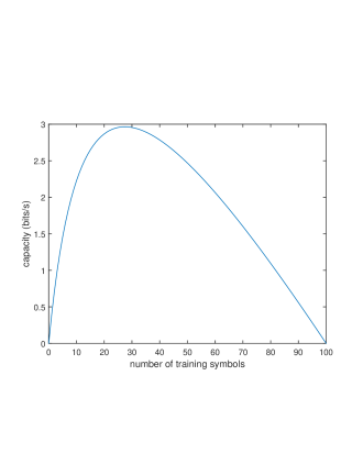
Refer to caption
Figure 1: A plot of the 2ร—1212\times 1 channel capacity as a function of the number of training symbols with tranmission power given by P=100๐‘ƒ100P=100.
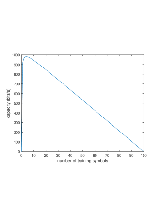
Refer to caption
Figure 2: A plot of the 2ร—1212\times 1 channel capacity as a function of the number of training symbols with tranmission power given by P=0.01๐‘ƒ0.01P=0.01.
Example 1

Consider a communication SIMO channel H๐ปH with perfect feedback and a randomly generated covariance matrix

C=(0.7426โˆ’0.7222โˆ’0.72226.4075)๐ถmatrix0.74260.72220.72226.4075C=\begin{pmatrix}0.7426&-0.7222\\ -0.7222&6.4075\end{pmatrix}

The length of the block is assumed to be T=100๐‘‡100T=100. Figure 1 shows that the optimum number of training symbols is Tฯ„=4subscript๐‘‡๐œ4T_{\tau}=4 when the power cosntraint is given by P=100๐‘ƒ100P=100, whereas for P=0.01๐‘ƒ0.01P=0.01, Figure 2 shows that the capacity is maximized for Tฯ„=27subscript๐‘‡๐œ27T_{\tau}=27, which is 27% of the available transmission power.

Example 2

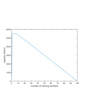
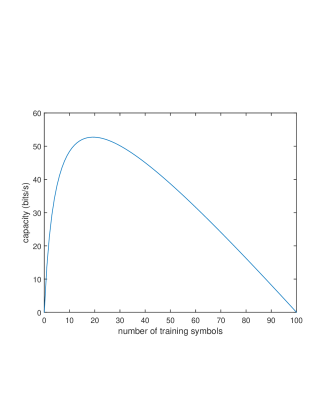
Consider a communication SIMO channel H๐ปH with perfect feedback and a randomly generated covariance matrix C๐ถC given in the appendix. The length of the block is assumed to be T=100๐‘‡100T=100. Figure 3 shows that the optimum number of training symbols is Tฯ„=2subscript๐‘‡๐œ2T_{\tau}=2 when the power cosntraint is given by P=100๐‘ƒ100P=100, whereas for P=0.01๐‘ƒ0.01P=0.01, Figure 4 shows that the capacity is maximized for Tฯ„=19subscript๐‘‡๐œ19T_{\tau}=19. The example clearly shows that the number of pilots needed is smaller when the number of receiving antennas increases. This is because of the increasement of the received signal power which makes the system less sensitive to channel estimation errors.
Refer to caption
Figure 3: A plot of the 10ร—110110\times 1 channel capacity as a function of the number of training symbols with tranmission power given by P=100๐‘ƒ100P=100.
Refer to caption
Figure 4: A plot of the 10ร—110110\times 1 channel capacity as a function of the number of training symbols with tranmission power given by P=0.01๐‘ƒ0.01P=0.01.

VI Asymptotic Results

The previous numerical examples clearly show the the dependence of the number of training symbols on the the symbol transmit power. We may understand this relation by looking at the asymptotic results when the power P๐‘ƒP tends to 00 or infinity (low respectively high signal to noise ratio). Recall that the covariance of the channel estimation error is given by

C~=1Tฯ„โ€‹(Pโ€‹C+1Tฯ„โ€‹Im)โˆ’1โ€‹C~๐ถ1subscript๐‘‡๐œsuperscript๐‘ƒ๐ถ1subscript๐‘‡๐œsubscript๐ผ๐‘š1๐ถ\tilde{C}=\frac{1}{T_{\tau}}\left(PC+\frac{1}{T_{\tau}}I_{m}\right)^{-1}C

Cleary, if P๐‘ƒP is very small and Tฯ„subscript๐‘‡๐œT_{\tau} is small, then 1Tฯ„โ€‹Imโ‰ปPโ€‹Csucceeds1subscript๐‘‡๐œsubscript๐ผ๐‘š๐‘ƒ๐ถ\frac{1}{T_{\tau}}I_{m}\succ PC, and so Pโ€‹C+1Tฯ„โ€‹Im๐‘ƒ๐ถ1subscript๐‘‡๐œsubscript๐ผ๐‘šPC+\frac{1}{T_{\tau}}I_{m} will be dominated by 1Tฯ„โ€‹Im1subscript๐‘‡๐œsubscript๐ผ๐‘š\frac{1}{T_{\tau}}I_{m}. Thus

C~โ†’1Tฯ„โ€‹(1Tฯ„โ€‹Im)โˆ’1โ€‹C=Cโ†’~๐ถ1subscript๐‘‡๐œsuperscript1subscript๐‘‡๐œsubscript๐ผ๐‘š1๐ถ๐ถ\tilde{C}\rightarrow\frac{1}{T_{\tau}}\left(\frac{1}{T_{\tau}}I_{m}\right)^{-1}C=C

as Pโ†’0โ†’๐‘ƒ0P\rightarrow 0. This implies that the capacity would tend to zero too. Therefore, for small P๐‘ƒP, the number of training symbols Tฯ„subscript๐‘‡๐œT_{\tau} must be large in order for 1Tฯ„โ€‹Im1subscript๐‘‡๐œsubscript๐ผ๐‘š\frac{1}{T_{\tau}}I_{m} to be of the same order as Pโ€‹C๐‘ƒ๐ถPC and so making C~~๐ถ\tilde{C} in some sense.

Now consider the other extreme, that is when P๐‘ƒP is large and recall the capacity formula

๐’žโ€‹(Tฯ„)๐’žsubscript๐‘‡๐œ\displaystyle\mathcal{C}(T_{\tau}) =(Tโˆ’Tฯ„)โ€‹(log2โ€‹det(Pโ€‹C+Im)โˆ’log2โ€‹det(Pโ€‹C~+Im))absent๐‘‡subscript๐‘‡๐œsubscript2๐‘ƒ๐ถsubscript๐ผ๐‘šsubscript2๐‘ƒ~๐ถsubscript๐ผ๐‘š\displaystyle=(T-T_{\tau})(\log_{2}{\det(PC+I_{m})}-\log_{2}{\det(P\tilde{C}+I_{m})})

In this case, we get 1Tฯ„โ€‹Imโ‰บPโ€‹Cprecedes1subscript๐‘‡๐œsubscript๐ผ๐‘š๐‘ƒ๐ถ\frac{1}{T_{\tau}}I_{m}\prec PC. Inspecting the formula for C~~๐ถ\tilde{C} again, we see that Pโ€‹C+1Tฯ„โ€‹Im๐‘ƒ๐ถ1subscript๐‘‡๐œsubscript๐ผ๐‘šPC+\frac{1}{T_{\tau}}I_{m} will be dominated by Pโ€‹C๐‘ƒ๐ถPC and thus

C~โ‰ˆ1Tฯ„โ€‹(Pโ€‹C)โˆ’1โ€‹C=1Tฯ„โ€‹P.~๐ถ1subscript๐‘‡๐œsuperscript๐‘ƒ๐ถ1๐ถ1subscript๐‘‡๐œ๐‘ƒ\tilde{C}\approx\frac{1}{T_{\tau}}\left(PC\right)^{-1}C=\frac{1}{T_{\tau}P}.

Hence,

log2โ€‹det(Pโ€‹C~+Im)subscript2๐‘ƒ~๐ถsubscript๐ผ๐‘š\displaystyle\log_{2}{\det(P\tilde{C}+I_{m})} โ‰ˆlog2โ€‹det(1Tฯ„โ€‹Im+Im)absentsubscript21subscript๐‘‡๐œsubscript๐ผ๐‘šsubscript๐ผ๐‘š\displaystyle\approx\log_{2}\det\left(\frac{1}{T_{\tau}}I_{m}+I_{m}\right)
=mโ€‹log2โก(1Tฯ„+1)absent๐‘šsubscript21subscript๐‘‡๐œ1\displaystyle=m\log_{2}\left(\frac{1}{T_{\tau}}+1\right)

Note also that for large P๐‘ƒP, we have that

log2โ€‹det(Pโ€‹C+Im)โ‰ˆlog2โ€‹det(Pโ€‹C).subscript2๐‘ƒ๐ถsubscript๐ผ๐‘šsubscript2๐‘ƒ๐ถ\log_{2}\det(PC+I_{m})\approx\log_{2}\det(PC).

So for large P๐‘ƒP, the capacity may be well approximated by

๐’žโ€‹(Tฯ„)๐’žsubscript๐‘‡๐œ\displaystyle\mathcal{C}(T_{\tau}) โ‰ˆ(Tโˆ’Tฯ„)โ€‹(log2โ€‹det(Pโ€‹C)โˆ’mโ€‹log2โก(1Tฯ„+1))absent๐‘‡subscript๐‘‡๐œsubscript2๐‘ƒ๐ถ๐‘šsubscript21subscript๐‘‡๐œ1\displaystyle\approx(T-T_{\tau})(\log_{2}{\det(PC)}-m\log_{2}\left(\frac{1}{T_{\tau}}+1\right))

We see that the capacity increases linearly with decreasing Tฯ„subscript๐‘‡๐œT_{\tau} while it increases logarithmically with increasing Tฯ„subscript๐‘‡๐œT_{\tau}. Therefore, the optimal choice of the number of training symbols Tฯ„โ†’1โ†’subscript๐‘‡๐œ1T_{\tau}\rightarrow 1 as Pโ†’โˆžโ†’๐‘ƒP\rightarrow\infty.

VII Conclusion

We considered the problem of deciding the power ratio between the training symbols and data symbols in order to maximize the channel capacity for transmission over uncertain channels with channel state information at the transmitter and receiver. We considered the worst case capacity as a performance measure, where the transceiver maximizes the minimal capacity over all distributions of the measurement noise with a fixed covariance known at both the transmitter and receiver. We presented an exact expression of the channel capacity as a function of the channel covariance matrix, the noise covariance matrix, and the number of training symbols used during a coherence time interval. This expression determines the number of training symbols that need to be used by finding the optimal integer number of training symbols that maximize the channel capacity. We also showed by means of numerical examples the trade-off between the number of training and data symbols. The results indicate that when the transmission power (or equivalently the signal to noise ratio) is high, a smaller number of training symbols is required to maximize the capacity compared to the low transmission power case. We confirm these observations theoretically considering the asymptotic behavior of the power as it grows large or decreases to very small values. Future work considers the general MIMO case, which is more involved due to combinatorial issues arising in choosing the number of training symbols for different transmitting antennas.

References

  • [1] G.ย Caire, N.ย Jindal, M.ย Kobayashi, and N.ย Ravindran. Multiuser MIMO achievable rates with downlink training and channel state feedback. Information Theory, IEEE Transactions on, 56(6):2845โ€“2866, June 2010.
  • [2] G.ย Fodor, P.ย Diย Marco, and M.ย Telek. Performance analysis of block and comb type channel estimation for massive mimo systems. In 5G for Ubiquitous Connectivity (5GU), 2014 1st International Conference on, pages 62โ€“69, Nov 2014.
  • [3] B.ย Hassibi and B.ย M. Hochwald. How much training is needed in multiple-antenna wireless links? Information Theory, IEEE Transactions on, 49(4):951โ€“963, April 2003.
  • [4] R.ย A. Horn and C.ย R. Johnson. Topics in Matrix Analysis. Cambridge University Press, 1991.
  • [5] R.ย A. Horn and C.ย R. Johnson. Matrix Analysis. Cambridge University Press, 1999.
  • [6] T.ย L. Marzetta and B.M. Hochwald. Capacity of a mobile multiple-antenna communication link in Rayleigh flat fading. Information Theory, IEEE Transactions on, 45(1):139โ€“157, Jan 1999.
  • [7] I.ย Emre Telatar. Capacity of multi-antenna Gaussian channels. European Transactions on Telecommunications, 10(6):585โ€“595, 1999.

Proof of Theorem 1

Define

๐’žโ‹†=supydโˆผ๐’žโ€‹๐’ฉโ€‹(0,XdโŠ—C+Wd)infvdโˆผ๐’žโ€‹๐’ฉโ€‹(0,Vd)Vd=Imโ€‹Td+XdโŠ—C~Iโ€‹(xd;yd)subscript๐’žโ‹†subscriptsupremumsimilar-tosubscript๐‘ฆ๐‘‘๐’ž๐’ฉ0tensor-productsubscript๐‘‹๐‘‘๐ถsubscript๐‘Š๐‘‘subscriptinfimumsimilar-tosubscript๐‘ฃ๐‘‘๐’ž๐’ฉ0subscript๐‘‰๐‘‘subscript๐‘‰๐‘‘subscript๐ผ๐‘šsubscript๐‘‡๐‘‘tensor-productsubscript๐‘‹๐‘‘~๐ถIsubscript๐‘ฅ๐‘‘subscript๐‘ฆ๐‘‘{\mathcal{C}}_{\star}=\sup_{y_{d}\sim{\mathcal{CN}}\left(0,X_{d}\otimes C+W_{d}\right)}\inf_{\begin{subarray}{c}v_{d}\sim{\mathcal{CN}}\left(0,V_{d}\right)\\ V_{d}=I_{mT_{d}}+X_{d}\otimes\tilde{C}\end{subarray}}\textup{I}(x_{d};y_{d}) (23)

and

๐’žยฏ=sup๐„โ€‹{xdโ€‹(t)โ€‹xdโˆ—โ€‹(t)}=Xdinfvdโˆผ๐’žโ€‹๐’ฉโ€‹(0,Vd)Vd=Imโ€‹Td+XdโŠ—C~Iโ€‹(xd;yd),ยฏ๐’žsubscriptsupremum๐„subscript๐‘ฅ๐‘‘๐‘กsuperscriptsubscript๐‘ฅ๐‘‘๐‘กsubscript๐‘‹๐‘‘subscriptinfimumsimilar-tosubscript๐‘ฃ๐‘‘๐’ž๐’ฉ0subscript๐‘‰๐‘‘subscript๐‘‰๐‘‘subscript๐ผ๐‘šsubscript๐‘‡๐‘‘tensor-productsubscript๐‘‹๐‘‘~๐ถIsubscript๐‘ฅ๐‘‘subscript๐‘ฆ๐‘‘\overline{\mathcal{C}}=\sup_{{\mathbf{E}}\left\{x_{d}(t)x_{d}^{*}(t)\right\}=X_{d}}\inf_{\begin{subarray}{c}v_{d}\sim{\mathcal{CN}}\left(0,V_{d}\right)\\ V_{d}=I_{mT_{d}}+X_{d}\otimes\tilde{C}\end{subarray}}\textup{I}(x_{d};y_{d}), (24)

Let the estimator at the receiver be a linear function of the received signal ydsubscript๐‘ฆ๐‘‘y_{d}, that is the estimate of xdsubscript๐‘ฅ๐‘‘x_{d} is given by x^d=Ldโ€‹(H^dโ€‹xd+vd)subscript^๐‘ฅ๐‘‘subscript๐ฟ๐‘‘subscript^๐ป๐‘‘subscript๐‘ฅ๐‘‘subscript๐‘ฃ๐‘‘\hat{x}_{d}=L_{d}(\hat{H}_{d}x_{d}+v_{d}) for some matrix Ldโˆˆโ„Tdร—mโ€‹Tdsubscript๐ฟ๐‘‘superscriptโ„subscript๐‘‡๐‘‘๐‘šsubscript๐‘‡๐‘‘L_{d}\in\mathbb{R}^{T_{d}\times mT_{d}}. Since the receiver could be chosen nonlinear, we will get a lower bound on the capacity ๐’žโ€‹(Tฯ„)๐’žsubscript๐‘‡๐œ\mathcal{C}(T_{\tau}). Introduce x~d=xdโˆ’x^dsubscript~๐‘ฅ๐‘‘subscript๐‘ฅ๐‘‘subscript^๐‘ฅ๐‘‘\tilde{x}_{d}=x_{d}-\hat{x}_{d}. Then

๐’žโ‹†subscript๐’žโ‹†\displaystyle\mathcal{C}_{\star} =Iโ€‹(xd;yd)absentIsubscript๐‘ฅ๐‘‘subscript๐‘ฆ๐‘‘\displaystyle=\textup{I}(x_{d};y_{d}) (25)
=hโ€‹(xd)โˆ’hโ€‹(xd|yd)absentโ„Žsubscript๐‘ฅ๐‘‘โ„Žconditionalsubscript๐‘ฅ๐‘‘subscript๐‘ฆ๐‘‘\displaystyle=h(x_{d})-h(x_{d}|y_{d}) (26)
=hโ€‹(xd)โˆ’hโ€‹(x^d+x~d|yd)absentโ„Žsubscript๐‘ฅ๐‘‘โ„Žsubscript^๐‘ฅ๐‘‘conditionalsubscript~๐‘ฅ๐‘‘subscript๐‘ฆ๐‘‘\displaystyle=h(x_{d})-h(\hat{x}_{d}+\tilde{x}_{d}|y_{d}) (27)
โ‰ฅhโ€‹(xd)โˆ’hโ€‹(x~d)absentโ„Žsubscript๐‘ฅ๐‘‘โ„Žsubscript~๐‘ฅ๐‘‘\displaystyle\geq h(x_{d})-h(\tilde{x}_{d}) (28)

Thus,

infvdVd=Imโ€‹Td+XdโŠ—C~Iโ€‹(xd;yd)subscriptinfimumsubscript๐‘ฃ๐‘‘subscript๐‘‰๐‘‘subscript๐ผ๐‘šsubscript๐‘‡๐‘‘tensor-productsubscript๐‘‹๐‘‘~๐ถIsubscript๐‘ฅ๐‘‘subscript๐‘ฆ๐‘‘\displaystyle\inf_{\begin{subarray}{c}v_{d}\\ V_{d}=I_{mT_{d}}+X_{d}\otimes\tilde{C}\end{subarray}}\textup{I}(x_{d};y_{d}) =hโ€‹(xd)โˆ’hโ€‹(x~d)absentโ„Žsubscript๐‘ฅ๐‘‘โ„Žsubscript~๐‘ฅ๐‘‘\displaystyle=h(x_{d})-h(\tilde{x}_{d}) (29)

which is attained for vdsubscript๐‘ฃ๐‘‘v_{d} such that yd=H^dโ€‹xd+vdsubscript๐‘ฆ๐‘‘subscript^๐ป๐‘‘subscript๐‘ฅ๐‘‘subscript๐‘ฃ๐‘‘y_{d}=\hat{H}_{d}x_{d}+v_{d} is Gaussian, which implies in turn that x^d=Ldโ€‹(H^dโ€‹xd+vd)subscript^๐‘ฅ๐‘‘subscript๐ฟ๐‘‘subscript^๐ป๐‘‘subscript๐‘ฅ๐‘‘subscript๐‘ฃ๐‘‘\hat{x}_{d}=L_{d}(\hat{H}_{d}x_{d}+v_{d}) and x~dsubscript~๐‘ฅ๐‘‘\tilde{x}_{d} are Gaussian, and x~dsubscript~๐‘ฅ๐‘‘\tilde{x}_{d} is independent of ydsubscript๐‘ฆ๐‘‘y_{d}, so equality holds in (28). Also, hโ€‹(xd)โ„Žsubscript๐‘ฅ๐‘‘h(x_{d}) is maximized for xdsubscript๐‘ฅ๐‘‘x_{d} when itโ€™s Gaussian under a fixed covaraince. Hence, ๐’žโ€‹(Tฯ„)โ‰ฅ๐’žโ‹†.๐’žsubscript๐‘‡๐œsubscript๐’žโ‹†\mathcal{C}(T_{\tau})\geq\mathcal{C}_{\star}. Now consider an arbitrary receiver, that is not necessarily linear and suppose that vdsubscript๐‘ฃ๐‘‘v_{d} is Gaussian and independent of xdsubscript๐‘ฅ๐‘‘x_{d}. This gives the capacity upperbound ๐’žยฏโ‰ฅ๐’žโ€‹(Tฯ„)ยฏ๐’ž๐’žsubscript๐‘‡๐œ\overline{\mathcal{C}}\geq\mathcal{C}(T_{\tau}). We have that

Iโ€‹(xd;yd)Isubscript๐‘ฅ๐‘‘subscript๐‘ฆ๐‘‘\displaystyle\textup{I}(x_{d};y_{d}) =hโ€‹(yd)โˆ’hโ€‹(yd|xd)absentโ„Žsubscript๐‘ฆ๐‘‘โ„Žconditionalsubscript๐‘ฆ๐‘‘subscript๐‘ฅ๐‘‘\displaystyle=h(y_{d})-h(y_{d}|x_{d}) (30)
=hโ€‹(yd)โˆ’hโ€‹(vd|xd)absentโ„Žsubscript๐‘ฆ๐‘‘โ„Žconditionalsubscript๐‘ฃ๐‘‘subscript๐‘ฅ๐‘‘\displaystyle=h(y_{d})-h(v_{d}|x_{d}) (31)
=hโ€‹(yd)โˆ’hโ€‹(vd)absentโ„Žsubscript๐‘ฆ๐‘‘โ„Žsubscript๐‘ฃ๐‘‘\displaystyle=h(y_{d})-h(v_{d}) (32)

where the inequality (32) holds since vdsubscript๐‘ฃ๐‘‘v_{d} is assumed to be independent of xdsubscript๐‘ฅ๐‘‘x_{d}. Since hโ€‹(yd)โ„Žsubscript๐‘ฆ๐‘‘h(y_{d}) is maximized when ydsubscript๐‘ฆ๐‘‘y_{d} is Gaussian, we get ๐’žโ€‹(Tฯ„)โ‰ค๐’žยฏ=๐’žโ‹†.๐’žsubscript๐‘‡๐œยฏ๐’žsubscript๐’žโ‹†\mathcal{C}(T_{\tau})\leq\overline{\mathcal{C}}=\mathcal{C}_{\star}. Since we already have the inequality ๐’žโ€‹(Tฯ„)โ‰ฅ๐’žโ‹†๐’žsubscript๐‘‡๐œsubscript๐’žโ‹†\mathcal{C}(T_{\tau})\geq\mathcal{C}_{\star}, we conclude that ๐’žโ€‹(Tฯ„)=๐’žโ‹†๐’žsubscript๐‘‡๐œsubscript๐’žโ‹†\mathcal{C}(T_{\tau})=\mathcal{C}_{\star}, and clearly xdsubscript๐‘ฅ๐‘‘x_{d} and ydsubscript๐‘ฆ๐‘‘y_{d} Gaussian give the worst case capacity ๐’žโ€‹(Tฯ„)=๐’žโ‹†๐’žsubscript๐‘‡๐œsubscript๐’žโ‹†\mathcal{C}(T_{\tau})=\mathcal{C}_{\star}.

Now let the eigenvalue decompositions of Xdsubscript๐‘‹๐‘‘X_{d}, C๐ถC, and C~~๐ถ\tilde{C} be given by Xd=Uโ€‹ฮฃโ€‹Uโˆ—subscript๐‘‹๐‘‘๐‘ˆฮฃsuperscript๐‘ˆX_{d}=U\Sigma U^{*}, ฮฃ=diagโ€‹(ฯƒ1,โ€ฆ,ฯƒTd)ฮฃdiagsubscript๐œŽ1โ€ฆsubscript๐œŽsubscript๐‘‡๐‘‘\Sigma=\text{diag}(\sigma_{1},...,\sigma_{T_{d}}), C=Uยฏโ€‹ฮฃยฏโ€‹Uยฏโˆ—๐ถยฏ๐‘ˆยฏฮฃsuperscriptยฏ๐‘ˆC=\bar{U}\bar{\Sigma}\bar{U}^{*}, ฮฃยฏ=diagโ€‹(ฮฃยฏ1,โ€ฆ,ฮฃยฏTd)ยฏฮฃdiagsubscriptยฏฮฃ1โ€ฆsubscriptยฏฮฃsubscript๐‘‡๐‘‘\bar{\Sigma}=\text{diag}(\bar{\Sigma}_{1},...,\bar{\Sigma}_{T_{d}}), and C~=U~โ€‹ฮฃ~โ€‹U~โˆ—~๐ถ~๐‘ˆ~ฮฃsuperscript~๐‘ˆ\tilde{C}=\tilde{U}\tilde{\Sigma}\tilde{U}^{*}, ฮฃ~=diagโ€‹(ฯƒ~1,โ€ฆ,ฯƒ~Td)~ฮฃdiagsubscript~๐œŽ1โ€ฆsubscript~๐œŽsubscript๐‘‡๐‘‘\tilde{\Sigma}=\text{diag}(\tilde{\sigma}_{1},...,\tilde{\sigma}_{T_{d}}) . Then, the mutual information between the Gaussian input xdsubscript๐‘ฅ๐‘‘x_{d} and Gaussian output ydsubscript๐‘ฆ๐‘‘y_{d} satisfies

Iโ€‹(xd;yd)Isubscript๐‘ฅ๐‘‘subscript๐‘ฆ๐‘‘\displaystyle\textup{I}(x_{d};y_{d}) =hโ€‹(yd)โˆ’hโ€‹(yd|xd)absentโ„Žsubscript๐‘ฆ๐‘‘โ„Žconditionalsubscript๐‘ฆ๐‘‘subscript๐‘ฅ๐‘‘\displaystyle=h(y_{d})-h(y_{d}|x_{d}) (33)
=log2โ€‹det(XdโŠ—C+ImโŠ—ITd)absentsubscript2tensor-productsubscript๐‘‹๐‘‘๐ถtensor-productsubscript๐ผ๐‘šsubscript๐ผsubscript๐‘‡๐‘‘\displaystyle=\log_{2}{\det(X_{d}\otimes C+I_{m}\otimes I_{T_{d}})}
โˆ’log2โ€‹det(XdโŠ—C~+ImโŠ—ITd)subscript2tensor-productsubscript๐‘‹๐‘‘~๐ถtensor-productsubscript๐ผ๐‘šsubscript๐ผsubscript๐‘‡๐‘‘\displaystyle~{}~{}~{}-\log_{2}{\det(X_{d}\otimes\tilde{C}+I_{m}\otimes I_{T_{d}})} (34)
=log2โ€‹det(XdโŠ—C+Imโ€‹Td)absentsubscript2tensor-productsubscript๐‘‹๐‘‘๐ถsubscript๐ผ๐‘šsubscript๐‘‡๐‘‘\displaystyle=\log_{2}{\det(X_{d}\otimes C+I_{mT_{d}})}
โˆ’log2โ€‹det(XdโŠ—C~+Imโ€‹Td)subscript2tensor-productsubscript๐‘‹๐‘‘~๐ถsubscript๐ผ๐‘šsubscript๐‘‡๐‘‘\displaystyle~{}~{}~{}-\log_{2}{\det(X_{d}\otimes\tilde{C}+I_{mT_{d}})} (35)
=log2โ€‹det((UโŠ—Uยฏ)โ€‹(ฮฃโŠ—ฮฃยฏ)โ€‹(UโŠ—Uยฏ)โˆ—+Imโ€‹Td)absentsubscript2tensor-product๐‘ˆยฏ๐‘ˆtensor-productฮฃยฏฮฃsuperscripttensor-product๐‘ˆยฏ๐‘ˆsubscript๐ผ๐‘šsubscript๐‘‡๐‘‘\displaystyle=\log_{2}{\det((U\otimes\bar{U})(\Sigma\otimes\bar{\Sigma})(U\otimes\bar{U})^{*}+I_{mT_{d}})}
โˆ’log2โ€‹det((UโŠ—U~)โ€‹(ฮฃโŠ—ฮฃ~)โ€‹(UโŠ—U~)โˆ—+Imโ€‹Td)subscript2tensor-product๐‘ˆ~๐‘ˆtensor-productฮฃ~ฮฃsuperscripttensor-product๐‘ˆ~๐‘ˆsubscript๐ผ๐‘šsubscript๐‘‡๐‘‘\displaystyle~{}~{}~{}-\log_{2}{\det((U\otimes\tilde{U})(\Sigma\otimes\tilde{\Sigma})(U\otimes\tilde{U})^{*}+I_{mT_{d}})} (36)
=log2โ€‹det((UโŠ—Uยฏ)โˆ—โ€‹(UโŠ—Uยฏ)โ€‹(ฮฃโŠ—ฮฃยฏ)+Imโ€‹Td)absentsubscript2superscripttensor-product๐‘ˆยฏ๐‘ˆtensor-product๐‘ˆยฏ๐‘ˆtensor-productฮฃยฏฮฃsubscript๐ผ๐‘šsubscript๐‘‡๐‘‘\displaystyle=\log_{2}{\det((U\otimes\bar{U})^{*}(U\otimes\bar{U})(\Sigma\otimes\bar{\Sigma})+I_{mT_{d}})}
โˆ’log2โ€‹det((UโŠ—U~)โˆ—โ€‹(UโŠ—U~)โ€‹(ฮฃโŠ—ฮฃ~)+Imโ€‹Td)subscript2superscripttensor-product๐‘ˆ~๐‘ˆtensor-product๐‘ˆ~๐‘ˆtensor-productฮฃ~ฮฃsubscript๐ผ๐‘šsubscript๐‘‡๐‘‘\displaystyle~{}~{}~{}-\log_{2}{\det((U\otimes\tilde{U})^{*}(U\otimes\tilde{U})(\Sigma\otimes\tilde{\Sigma})+I_{mT_{d}})} (37)
=log2โ€‹det(ฮฃโŠ—ฮฃยฏ+Imโ€‹Td)absentsubscript2tensor-productฮฃยฏฮฃsubscript๐ผ๐‘šsubscript๐‘‡๐‘‘\displaystyle=\log_{2}{\det(\Sigma\otimes\bar{\Sigma}+I_{mT_{d}})}
โˆ’log2โ€‹det(ฮฃโŠ—ฮฃ~+Imโ€‹Td)subscript2tensor-productฮฃ~ฮฃsubscript๐ผ๐‘šsubscript๐‘‡๐‘‘\displaystyle~{}~{}~{}-\log_{2}{\det(\Sigma\otimes\tilde{\Sigma}+I_{mT_{d}})} (38)
=log2โก(โˆi=1Tddet(ฯƒiโ€‹ฮฃยฏ+Im))absentsubscript2superscriptsubscriptproduct๐‘–1subscript๐‘‡๐‘‘subscript๐œŽ๐‘–ยฏฮฃsubscript๐ผ๐‘š\displaystyle=\log_{2}{\left(\prod_{i=1}^{T_{d}}\det(\sigma_{i}\bar{\Sigma}+I_{m})\right)}
โˆ’log2โก(โˆi=1Tddet(ฯƒiโ€‹ฮฃ~+Im))subscript2superscriptsubscriptproduct๐‘–1subscript๐‘‡๐‘‘subscript๐œŽ๐‘–~ฮฃsubscript๐ผ๐‘š\displaystyle~{}~{}~{}-\log_{2}{\left(\prod_{i=1}^{T_{d}}\det(\sigma_{i}\tilde{\Sigma}+I_{m})\right)} (39)
=Tdlog2(โˆi=1Tddet(ฯƒiโ€‹ฮฃยฏ+Im)det(ฯƒiโ€‹ฮฃ~+Im))1Td\displaystyle=T_{d}\log_{2}\left(\prod_{i=1}^{T_{d}}\frac{\det(\sigma_{i}\bar{\Sigma}+I_{m})}{\det(\sigma_{i}\tilde{\Sigma}+I_{m})}\right)^{\frac{1}{T_{d}}} (40)
โ‰คTdโ€‹log2โก(1Tdโ€‹โˆ‘i=1Tddet(ฯƒiโ€‹ฮฃยฏ+Im)det(ฯƒiโ€‹ฮฃ~+Im))absentsubscript๐‘‡๐‘‘subscript21subscript๐‘‡๐‘‘superscriptsubscript๐‘–1subscript๐‘‡๐‘‘subscript๐œŽ๐‘–ยฏฮฃsubscript๐ผ๐‘šsubscript๐œŽ๐‘–~ฮฃsubscript๐ผ๐‘š\displaystyle\leq T_{d}\log_{2}\left(\frac{1}{T_{d}}\sum_{i=1}^{T_{d}}\frac{\det(\sigma_{i}\bar{\Sigma}+I_{m})}{\det(\sigma_{i}\tilde{\Sigma}+I_{m})}\right) (41)

where (36) follows from Proposition 1, (37) follows from Proposition 2, (38) follows from Proposition 1, and (41) follows from Proposition 3, with equality if and only if ฯƒ1=ฯƒ2=โ‹ฏ=ฯƒTdsubscript๐œŽ1subscript๐œŽ2โ‹ฏsubscript๐œŽsubscript๐‘‡๐‘‘\sigma_{1}=\sigma_{2}=\cdots=\sigma_{T_{d}}. Since ฯƒ1+ฯƒ2+โ‹ฏ+ฯƒTd=๐“๐ซโ€‹(ฮฃ)=๐“๐ซโ€‹(X)=nโ€‹Psubscript๐œŽ1subscript๐œŽ2โ‹ฏsubscript๐œŽsubscript๐‘‡๐‘‘๐“๐ซฮฃ๐“๐ซ๐‘‹๐‘›๐‘ƒ\sigma_{1}+\sigma_{2}+\cdots+\sigma_{T_{d}}={\mathbf{Tr}}\left(\Sigma\right)={\mathbf{Tr}}\left(X\right)=nP, we must have

ฯƒ1=ฯƒ2=โ‹ฏ=ฯƒTd=Psubscript๐œŽ1subscript๐œŽ2โ‹ฏsubscript๐œŽsubscript๐‘‡๐‘‘๐‘ƒ\sigma_{1}=\sigma_{2}=\cdots=\sigma_{T_{d}}=P

This implies that the capacity maximizing input covariance is X=Pโ‹…ITd๐‘‹โ‹…๐‘ƒsubscript๐ผsubscript๐‘‡๐‘‘X=P\cdot I_{T_{d}}. Thus, the maximum capacity is given by

๐’žโ€‹(Tฯ„)๐’žsubscript๐‘‡๐œ\displaystyle\mathcal{C}(T_{\tau}) =log2โ€‹det((Pโ€‹ITd)โŠ—(C^+C~)+ImโŠ—ITd)absentsubscript2tensor-product๐‘ƒsubscript๐ผsubscript๐‘‡๐‘‘^๐ถ~๐ถtensor-productsubscript๐ผ๐‘šsubscript๐ผsubscript๐‘‡๐‘‘\displaystyle=\log_{2}{\det((PI_{T_{d}})\otimes(\hat{C}+\tilde{C})+I_{m}\otimes I_{T_{d}})}
โˆ’log2โ€‹det((Pโ€‹ITd)โŠ—C~+ImโŠ—ITd)subscript2tensor-product๐‘ƒsubscript๐ผsubscript๐‘‡๐‘‘~๐ถtensor-productsubscript๐ผ๐‘šsubscript๐ผsubscript๐‘‡๐‘‘\displaystyle~{}~{}~{}-\log_{2}{\det((PI_{T_{d}})\otimes\tilde{C}+I_{m}\otimes I_{T_{d}})} (42)
=Td(log2det(PC+Im)\displaystyle=T_{d}(\log_{2}{\det(PC+I_{m})}
โˆ’log2det(PC~+Im))\displaystyle~{}~{}~{}-\log_{2}{\det(P\tilde{C}+I_{m})}) (43)
=(Tโˆ’Tฯ„)(log2det(PC+Im)\displaystyle=(T-T_{\tau})(\log_{2}{\det(PC+I_{m})}
โˆ’log2det(PC~+Im))\displaystyle~{}~{}~{}-\log_{2}{\det(P\tilde{C}+I_{m})}) (44)

and the proof is complete.

Supplement for Example 2

The random matrix C๐ถC used in Example 2 is given by

C๐ถ\displaystyle C =(12.618โˆ’2.5315โˆ’2.24241.1965โˆ’1.5896โˆ’2.53158.76392.0577โˆ’4.38892.0117โˆ’2.24242.05776.09970.2384โˆ’1.18941.1965โˆ’4.38890.23847.3271.1523โˆ’1.58962.0117โˆ’1.18941.152310.26432.5086โˆ’0.011โˆ’1.60820.35831.3222โˆ’4.5906โˆ’0.499โˆ’4.57640.705โˆ’0.1717โˆ’1.3983.1713โˆ’2.319โˆ’5.3612โˆ’2.3611.93452.1956โˆ’0.6284โˆ’2.2747โˆ’0.6889โˆ’4.07980.2636โˆ’0.5846โˆ’0.77511.2117\displaystyle=\left(\begin{matrix}12.618&-2.5315&-2.2424&1.1965&-1.5896\\ -2.5315&8.7639&2.0577&-4.3889&2.0117\\ -2.2424&2.0577&6.0997&0.2384&-1.1894\\ 1.1965&-4.3889&0.2384&7.327&1.1523\\ -1.5896&2.0117&-1.1894&1.1523&10.2643\\ 2.5086&-0.011&-1.6082&0.3583&1.3222\\ -4.5906&-0.499&-4.5764&0.705&-0.1717\\ -1.398&3.1713&-2.319&-5.3612&-2.361\\ 1.9345&2.1956&-0.6284&-2.2747&-0.6889\\ -4.0798&0.2636&-0.5846&-0.7751&1.2117\end{matrix}\right.
2.5086โˆ’4.5906โˆ’1.3981.9345โˆ’4.0798โˆ’0.011โˆ’0.4993.17132.19560.2636โˆ’1.6082โˆ’4.5764โˆ’2.319โˆ’0.6284โˆ’0.58460.35830.705โˆ’5.3612โˆ’2.2747โˆ’0.77511.3222โˆ’0.1717โˆ’2.361โˆ’0.68891.21172.13660.2868โˆ’0.86281.2528โˆ’1.13110.286818.432310.96092.38832.0394โˆ’0.862810.960920.496910.57051.32171.25282.388310.57059.7425โˆ’0.307โˆ’1.13112.03941.3217โˆ’0.3073.3511)\displaystyle~{}~{}~{}~{}~{}~{}\left.\begin{matrix}2.5086&-4.5906&-1.398&1.9345&-4.0798\\ -0.011&-0.499&3.1713&2.1956&0.2636\\ -1.6082&-4.5764&-2.319&-0.6284&-0.5846\\ 0.3583&0.705&-5.3612&-2.2747&-0.7751\\ 1.3222&-0.1717&-2.361&-0.6889&1.2117\\ 2.1366&0.2868&-0.8628&1.2528&-1.1311\\ 0.2868&18.4323&10.9609&2.3883&2.0394\\ -0.8628&10.9609&20.4969&10.5705&1.3217\\ 1.2528&2.3883&10.5705&9.7425&-0.307\\ -1.1311&2.0394&1.3217&-0.307&3.3511\end{matrix}\right)