Tilting Jupiter (a bit) and Saturn (a lot) During
Planetary Migration

Abstract

We study the effects of planetary late migration on the gas giants obliquities. We consider the planetary instability models from Nesvorný & Morbidelli (2012), in which the obliquities of Jupiter and Saturn can be excited when the spin-orbit resonances occur. The most notable resonances occur when the $s_{7}$ and $s_{8}$ frequencies, changing as a result of planetary migration, become commensurate with the precession frequencies of Jupiter’s and Saturn’s spin vectors. We show that Jupiter may have obtained its present obliquity by crossing of the $s_{8}$ resonance. This would set strict constrains on the character of migration during the early stage. Additional effects on Jupiter’s obliquity are expected during the last gasp of migration when the $s_{7}$ resonance was approached. The magnitude of these effects depends on the precise value of the Jupiter’s precession constant. Saturn’s large obliquity was likely excited by capture into the $s_{8}$ resonance. This probably happened during the late stage of planetary migration when the evolution of the $s_{8}$ frequency was very slow, and the conditions for capture into the spin-orbit resonance with $s_{8}$ were satisfied. However, whether or not Saturn is in the spin-orbit resonance with $s_{8}$ at the present time is not clear, because the existing observations of Saturn’s spin precession and internal structure models have significant uncertainties.

1 Introduction

It is believed that the orbital architecture of the solar system was significantly altered from its initial state after the dissipation of the protosolar nebula. The present architecture is probably a result of complex dynamical interaction between planets, and between planets and planetesimals left behind by planet formation. This becomes apparent because much of what we see in the solar system today can be explained if planets radially migrated, and/or if they evolved through a dynamical instability and reconfigured to a new state (e.g., Malhotra, 1995; Thommes et al., 1999; Tsiganis et al., 2005).

While details of this process are not known exactly, much has been learned about it over decade by testing various migration/instability models against various constraints. Some of the most important constraints are provided by the terrestrial planets and the populations of small bodies in the asteroid and Kuiper belts (e.g., Gomes et al., 2005; Minton & Malhotra, 2009, 2011; Levison et al., 2008; Morbidelli et al., 2010; Nesvorný, 2015). Processes related to the giant planet instability/migration were also used to explain capture and orbital distribution of Jupiter and Neptune Trojans (e.g., Morbidelli et al., 2005; Nesvorný & Vokrouhlický, 2009; Nesvorný et al., 2014a) and irregular satellites (e.g., Nesvorný et al., 2007, 2014b). Some of the most successful instability/migration models developed so far postulate that the outer solar system contained additional ice giant that was ejected into interstellar space by Jupiter (e.g., Nesvorný, 2011; Nesvorný & Morbidelli, 2012; Batygin et al., 2012). The orbits of the four surviving giant planets evolved in this model by planetesimal-driven migration and by scattering encounters with the ejected planet. In this work, we use this framework to investigate the behavior of Jupiter’s and Saturn’s obliquities.

The obliquity, $\varepsilon$, is the angle between the spin axis of a planet and the normal to its orbital plane. The core accretion theory applied to Jupiter and Saturn implies that their primordial obliquities should be very small. This is because the angular momentum of the rotation of these planets is contained almost entirely in their massive hydrogen and helium envelopes. The stochastic accretion of solid cores should therefore be irrelevant for their current obliquity values (see Lissauer & Safronov 1991 for a discussion), and a symmetric inflow of gas on forming planets should lead to $\varepsilon\simeq 0$. The present obliquity of Jupiter is $\varepsilon_{\rm J}=3.1^{\circ}$, which is small, but not quite small enough for these expectations, but that of Saturn is $\varepsilon_{\rm S}=26.7^{\circ}$, which is clearly not.

Ward & Hamilton (2004) and Hamilton & Ward (2004) noted that the precession frequency of Saturn’s spin axis has a value close to $s_{8}\simeq-0.692$ arcsec yr^-1, where $s_{8}$ is the mean nodal regression of Neptune’s orbit (or, equivalently, the eighth nodal eigenfrequency of the planetary system; e.g., Applegate et al. 1986; Laskar 1988). Similarly, Ward & Canup (2006) pointed out that the precession frequency of Jupiter’s spin axis has a value close to $s_{7}\simeq-2.985$ arcsec yr^-1, where $s_{7}$ is the mean nodal regression of Uranus’s orbit. These findings are significant because they raise the possibility that the current obliquities of Jupiter and Saturn have something to do with the precession of the giant planet orbits. Specifically, Ward & Hamilton (2004) and Hamilton & Ward (2004) suggested that the present value of Saturn’s obliquity can be explained by capture of Saturn’s spin vector in a resonance with $s_{8}$. They proposed that the capture occurred when Saturn’s spin vector precession increased as a result of Saturn’s cooling and contraction, or because $s_{8}$ decreased during the depletion of the primordial Kuiper belt. They showed that, if the post-capture evolution is conveniently slow, the spin-orbit resonance (also known as the Cassini resonance, see Section 2) is capable of increasing Saturn’s obliquity to its current value.

While changes of precession or $s_{8}$ during the earliest epochs could have been important, it seems more likely that capture in the spin-orbit resonance occurred later, probably as a result of planetary migration (Boué et al., 2009). This is because both $s_{7}$ and $s_{8}$ significantly change during the instability and subsequent migration. Therefore, if the spin-orbit resonances had been established earlier, they would not survive to the present time. Boué et al. (2009) studied various scenarios for resonant tilting of Saturn’s spin axis during the planetary migration and found that the present obliquity of Saturn can be explained only if the characteristic migration time scale was long and/or if Neptune’s inclination was substantially excited during the instability. Since Neptune inclination is never large in the instability/migration models of Nesvorný & Morbidelli (2012; hereafter NM12), typically $i_{\rm N}<1^{\circ}$, the migration timescales presumably need (note that Boué et al. (2009) did not investigated these low-$i$ cases in detail) to be very long (see Section 3.3). Interestingly, these very long migration timescales are also required from other constraints (e.g., Morbidelli et al., 2014; Nesvorný, 2015). They could be achieved in the Nesvorný & Morbidelli (2012) models if Neptune interacted with an already depleted planetesimal disk during the very last stages of the migration process. As for the obliquity of Jupiter, Ward & Canup (2006) suggested that the present value is due to the proximity of the spin precession rate to the $s_{7}$ frequency.

In fact, the obliquities of Jupiter and Saturn represent a much stronger constraint on the instability/migration models than was realized before. This is because the constraints from the present obliquities of Jupiter and Saturn must be satisfied simultaneously (McNeil & Lee 2010; Brasser & Lee 2015). For example, in the initial configuration of planets in the NM12 models, the $s_{8}$ frequency is much faster than the precession constants of both Jupiter and Saturn. This means that the $s_{8}$ mode, before approaching Saturn’s precession frequency and exciting its obliquity, must also have evolved over the precession frequency of Jupiter’s spin vector. This leads to a conundrum, because if the crossing were slow, Jupiter’s obliquity would increase as a result of capture into the spin-orbit resonance with $s_{8}$. If, on the other hand, the general evolution at all stages were fast, the conditions for capture of Saturn into the spin-orbit resonance with $s_{8}$ may not be be met (e.g., Boué et al., 2009), and Saturn’s obliquity would stay small.

A potential solution of this problem would be to invoke fast evolution of $s_{8}$ early on, during the crossing of Jupiter’s precession frequency, and slow evolution of $s_{8}$ later on, such that Saturn’s spin vector can be captured into the spin-orbit resonance with $s_{8}$ during the late stages. This can be achieved, for example, if the migration of the outer planets was faster before the instability, and slowed down later, as the outer Solar System progressed toward a more relaxed state. As we show in Section 3.1, the jumping-Jupiter models developed in NM12 provide a natural quantitative framework to study this possibility.

In Sec. 2 we first briefly review the general equations for the spin-orbit dynamics. Then, in Sec. 3, we investigate the behavior of the spin vectors of Jupiter and Saturn in the instability/migration models of NM12. We find that the constraints posed by Jupiter’s and Saturn’s obliquities can be satisfied simultaneously in this class of models, and derive detailed conditions on the migration timescales and precession constants that would provide a consistent solution.

2 Methods

2.1 Parametrization using non-singular spin vector components

Consider a planet revolving about the Sun and rotating with angular velocity $\omega$ about an instantaneous spin axis characterized by a unit vector ${\bf s}$. With solar gravitational torques applied on the planet, $\omega$ remains constant, but ${\bf s}$ evolves in the inertial space according to (e.g., Colombo, 1966)

$$\frac{d{\bf s}}{dt}=-\alpha\left({\bf c}\cdot{\bf s}\right)\left({\bf c}\times{\bf s}\right),$$ (1)

where ${\bf c}$ denotes a unit vector along the orbital angular momentum, and

$$\alpha=\frac{3}{2}\frac{GM_{\odot}}{\omega\,b^{3}}\frac{J_{2}+q}{\lambda+l}$$ (2)

is the precession constant of the planet. Here, $G$ is the gravitational constant, $M_{\odot}$ is the mass of the Sun, $b=a\sqrt{1-e^{2}}$, where $a$ and $e$ are the orbital semimajor axis and eccentricity, $J_{2}$ is the quadrupole coefficient of the planetary gravity field, and $\lambda=C/MR^{2}$ is the planetary moment of inertia $C$ normalized by a standard factor $MR^{2}$, where $M$ is planet’s mass and $R$ its reference radius (to be also used in the definition of $J_{2}$). The term $q=\text@frac{1}{2}\sum_{j}(m_{j}/M)(a_{j}/R)^{2}$ is an effective, long-term contribution to the quadrupole coefficient due to the massive, close-in regular satellites with masses $m_{j}$ and planetocentric distances $a_{j}$, and $l=\sum_{j}(m_{j}a_{j}^{2}n_{j})/(MR^{2}\omega)$ is the angular momentum content of the satellite orbits ($n_{j}$ denotes their planetocentric mean motion) normalized to the characteristic value of the planetary rotational angular momentum.

For both Jupiter and Saturn, $q$ is slightly dominant over $J_{2}$ in the numerator of the last term in Eq. (2), while $l$ is negligible in comparison to $\lambda$ in the denominator. Spacecraft observations have been used to accurately determine the values of $J_{2}$, $q$ and $l$. On the other hand, $\lambda$ cannot be derived in a straightforward manner from observations, because it depends on the structure of planetary interior. Using models of planetary interior, Helled et al. (2011) determined that Jupiter’s $\lambda_{\rm J}$ is somewhere in the range between $0.2513$ and $0.2529$ (here rescaled for the equatorial radius $R=71,492$ km of the planet). This would imply Jupiter’s precession constant $\alpha_{\rm J}$ to be in the range between $2.754$ arcsec yr^-1 and $2.772$ arcsec yr^-1. These values are smaller than the ones considered in Ward & Canup (2006), if their proposed small angular distance between Jupiter’s pole and Cassini state C₂ is correct.

Similarly, Helled et al. (2009) determined Saturn’s precession constant $\alpha_{\rm S}$ to be in the range between $0.8443$ arcsec yr^-1 and $0.8447$ arcsec yr^-1. Again, these values differ from those inferred by Ward & Hamilton (2004) and Hamilton & Ward (2004), if a resonant confinement of the Saturn’s spin axis in their proposed scenario is true. This difference has been noted and discussed in Boué et al. (2009). If Helled’s values are correct, Saturn’s spin axis cannot be presently locked in the resonance with $s_{8}$. However, it seems possible that of $\alpha_{\rm S}$ derived in Helled et al. (2009) may have somewhat larger uncertainty than reflected by the formal range of the inferred $\lambda$ values. Also, the interpretation is complicated by the past orbital evolution of planetary satellites which may have also contributed to changes of $\alpha_{\rm S}$ (and $\alpha_{\rm J}$). For these reason, and in the spirit of previous studies (e.g., Ward & Hamilton, 2004; Ward & Canup, 2006; Boué et al., 2009), here we consider a wider range of the precession constant values $\alpha$ for both Jupiter and Saturn.

Assuming $\alpha$ constant for a moment, a difficult element preventing a simple solution of Eq. (1) is the time evolution of ${\bf c}$. This is because mutual planetary interactions make their orbits precess in space on a characteristic timescale of tens of thousands of years and longer. In addition, during the early phase of planetary evolution, the precession rates of planetary orbits may have been faster due to the gravitational torques from a massive population of planetesimals in the trans-Neptunian disk. In the Keplerian parametrization of orbits, the unit vector ${\bf c}$ depends on the inclination $I$ and longitude of node $\Omega$, such that ${\bf c}^{T}=(\sin I\sin\Omega,-\sin I\cos\Omega,\cos I)$. Traditionally, the difficulties with the time dependence in Eq. (1) are resolved using a transformation to a reference frame fixed on an orbit, where ${\bf c}^{T}=(0,0,1)$.

The transformation from the inertial to orbit coordinate frames is achieved by applying a 3-1-3 rotation sequence with the Eulerian angles $(\Omega,I,-\Omega)$. This transforms Eq. (1) to the following form

$$\frac{d{\bf s}}{dt}=-\left[\alpha\left({\bf c}\cdot{\bf s}\right){\bf c}+{\bf h}\right]\times{\bf s},$$ (3)

where now the planetary spin vector ${\bf s}$ is expressed with respect to the orbit frame, and ${\bf c}$ is now a unit vector along the z-axis. In effect, the time dependence has been moved to the vector quantity ${\bf h}^{T}=(\mathcal{A},\mathcal{B},-2\mathcal{C})$ with

$${\mathcal{A}} \!\!\!=\!\!\! \cos\Omega\,{\dot{I}}-\sin I\sin\Omega\,{\dot{\Omega}},$$ (4a)

$${\mathcal{B}} \!\!\!=\!\!\! \sin\Omega\,{\dot{I}}+\sin I\cos\Omega\,{\dot{\Omega}},$$ (4b)

$${\mathcal{C}} \!\!\!=\!\!\! \sin^{2}I/2\,{\dot{\Omega}},$$ (4c)

and the over-dots mean time derivative.

A further development consists in introducing complex and non-singular parameter $\zeta=\sin(I/2)\,\exp(\imath\Omega)$ ($\imath=\sqrt{-1}$ is the complex unit) that replaces $I$ and $\Omega$. First order perturbation theory for quasi-circular and near-coplanar orbits indicates $\zeta$ for each planet can be expressed using a finite number of the Fourier terms with the $s_{i}$ frequencies uniquely dependent on the orbital semimajor axes and masses of the planets, and amplitudes set by the initial conditions (e.g., Brouwer & Clemence, 1961). In the models from non-linear theories or numerical integrations, $\zeta$ can still be represented by the Fourier expansion $\zeta=\sum A_{i}\exp[\imath(s_{i}t+\phi_{i})]$ (e.g., Applegate et al., 1986; Laskar, 1988), with the linear terms having typically the largest amplitudes $A_{i}$.

As discussed in Section 1, terms with present frequencies $s_{7}\simeq-2.985$ arcsec yr^-1 and $s_{8}\simeq-0.692$ arcsec yr^-1 are of a particular importance in this work. The $s_{7}$-term is the largest in Uranus’ $\zeta$ representation, and the $s_{8}$-term is the largest in Neptune’s $\zeta$ representation, and these terms also appear, though with smaller amplitudes, in the $\zeta$ variable of Jupiter and Saturn, because mutual planetary interactions enforce all fundamental frequency terms to appear in all planetary orbits. In terms of $\zeta$, Eqs. (4a-c) become

$$\mathcal{A}+\imath\,\mathcal{B} \!\!\!=\!\!\! \frac{2}{\sqrt{1-\zeta{\bar{\zeta}}}}\left(\frac{d\zeta}{dt}-\imath\zeta\,\mathcal{C}\right),$$ (5a)

$$\mathcal{C} \!\!\!=\!\!\! \frac{1}{2\imath}\left({\bar{\zeta}}\,\frac{d\zeta}{dt}-\zeta\,\frac{d{\bar{\zeta}}}{dt}\right),$$ (5b)

where ${\bar{\zeta}}$ is complex conjugate to $\zeta$. For small inclinations, relevant to this work, we therefore find that $\mathcal{A}+\imath\,\mathcal{B}\simeq 2\,(d\zeta/dt)$, and $\mathcal{C}\simeq 0$.

Another important aspect is of the problem is that Eq. (3) derives from a Hamiltonian

$$\mathcal{H}({\bf s};t)=\frac{\alpha}{2}\left({\bf c}\cdot{\bf s}\right)^{2}+{\bf h}\cdot{\bf s},$$ (6)

such that

$$\frac{d{\bf s}}{dt}=-\nabla_{\bf s}\mathcal{H}\times{\bf s}.$$ (7)

This allowed Breiter et al. (2005) to construct an efficient Lie-Poisson integrator for a fast propagation of the secular evolution of planetary spins. In Section 3, we will use the leap-frog variant of the Hamiltonian’s LP2 splitting from Breiter et al. (2005). To propagate ${\bf s}$ through a single integration step, Breiter et al. (2005) method requires that the orbital semimajor axis, eccentricity and ${\bf c}$ are provided at times corresponding to the beginning and end of the step. These values can be supplied from an analytic model of orbit evolution, or be directly obtained from a previous numerical integrations of orbits where $a$, $e$ and ${\bf c}$ were recorded with a conveniently dense sampling.

2.2 Parametrization using obliquity and precession angle

The Hamiltonian formulation in Eq. (6) allows us to introduce several important concepts of the Cassini dynamics. A long tradition in astronomy is to represent ${\bf s}$ with obliquity $\varepsilon$ and precession angle $\psi$ such that ${\bf s}^{T}=(\sin\varepsilon\sin\psi,\sin\varepsilon\cos\psi,\cos\varepsilon)$. The benefit of this parametrization is that the unit spin vector is expressed using only two variables. The drawback is that resulting equations are singular when $\varepsilon=0$.

The conjugated momentum to $\psi$ is $X=\cos\varepsilon$. The Hamiltonian is then (e.g., Laskar & Robutel, 1993)

$$\mathcal{H}(X,\psi;t) = \frac{\alpha}{2}X^{2}-2\mathcal{C}X$$

$$+\sqrt{1-X^{2}}\left(\mathcal{A}\sin\psi+\mathcal{B}\cos\psi\right).$$

For the low-inclination orbits, $\mathcal{C}$ is negligible, while $\mathcal{A}$ and $\mathcal{B}$ are expanded in the Fourier series with the same frequency terms as those appearing in $\zeta$ itself. A model of fundamental importance, introduced by G. Colombo (Colombo, 1966; Henrard & Murigande, 1987; Ward & Hamilton, 2004), is obtained when only one Fourier term in $\mathcal{A}$ and $\mathcal{B}$ is considered. This Colombo model obviously serves only as an approximation of the complete spin axis evolution, since all other Fourier terms in $\mathcal{A}$ and $\mathcal{B}$ act as a perturbation. Nevertheless, the Colombo model allows us to introduce several important concepts that are the basis of the discussion in Section 3.

In the Colombo model, the orbital inclination is fixed and the node precesses with a constant frequency. Put in a compact way, $\zeta=A\exp[\imath(st+\phi)]$ is the single Fourier term, and $A=\sin I/2$ and $\Omega=st+\phi$. Transformation to new canonical variables $X^{\prime}=-X$ and $\varphi=-(\psi+\Omega)$, and scaling with the nodal frequency $s$, results in a time-independent Hamiltonian

$$\mathcal{H}(X^{\prime},\varphi) = \kappa X^{\prime 2}-\cos IX^{\prime}$$

$$+\sin I\sqrt{1-X^{\prime 2}}\cos\varphi,$$

where $\kappa=\alpha/(2s)$ is a dimensionless parameter. Note that the orbit-plane angle $\varphi$ is measured from a reference direction that is $90^{\circ}$ ahead of the ascending node. The general structure of the phase flow of solutions $\mathcal{H}(X^{\prime},\varphi)=C$, with $C$ constant, derives from the location of the stationary points. Depending on the parameter values $(\kappa,I)$, there are either two ($|\kappa|<\kappa_{\star}$) or four ($|\kappa|>\kappa_{\star}$) such stationary solutions (called the Cassini states). The critical value of $\kappa$ reads (e.g., Henrard & Murigande, 1987)

$$\kappa_{\star}(I)=\frac{1}{2}\left(\sin^{2/3}I+\cos^{2/3}I\right)^{3/2}.$$ (10)

Therefore, for small $I$, $\kappa_{\star}\simeq\text@frac{1}{2}$. The stationary solutions are located at $\varphi=0^{\circ}$ or $\varphi=180^{\circ}$ meridians in the orbital frame, and have obliquity values given by a transcendental equation

$$\kappa\sin 2\varepsilon=-\sin\left(\varepsilon\mp I\right),$$ (11)

with the upper sign for $\varphi=0^{\circ}$, and the lower sign for $\varphi=180^{\circ}$.

In the present work, we are mainly interested in the Cassini state C₂ located at $\varphi=0^{\circ}$. For Jupiter, the C₂ state related to frequency $s=s_{7}$ is subcritical since $|\kappa|<\text@frac{1}{2}$ for all estimates of the Jupiter’s precession constant found in the literature. Only two Cassini states exist in this regime, and ${\bf s}$ must circulate about C₂. In the case of Saturn, $|\kappa|>\kappa_{\star}\simeq\text@frac{1}{2}$ for $s=s_{8}$, four Cassini states exist in this situation, and ${\bf s}$ was suggested to librate in the resonant zone about C₂. The configuration of vectors in C₂ can be inferred from Eq. (11). If the inclination is significantly smaller than the obliquity $\varepsilon$, we have that $\alpha\cos\varepsilon\simeq-s$. Since the term on the left hand side of this relation is the precession frequency of the planet’s spin (see Eq. 1), we find that the spin and orbit vectors will co-precess with the same rate about the normal vector to the inertial frame. Small resonant librations about C₂ would reveal themselves by small departures of the spin vector from this ideal state. The maximum width $\Delta\varepsilon$ of the resonant zone in obliquity at the $\varphi=0^{\circ}$ meridian can be obtained using an analytic formula (e.g., Henrard & Murigande, 1987)

$$\sin\frac{\Delta\varepsilon}{2}=\frac{1}{|\kappa|}\sqrt{\frac{\sin 2I}{\sin 2\varepsilon_{4}}},$$ (12)

where $\varepsilon_{4}$ is the obliquity of the unstable Cassini state C₄ (a solution of Eq. (11) at $\varphi=180^{\circ}$ having the intermediate value of the obliquity).

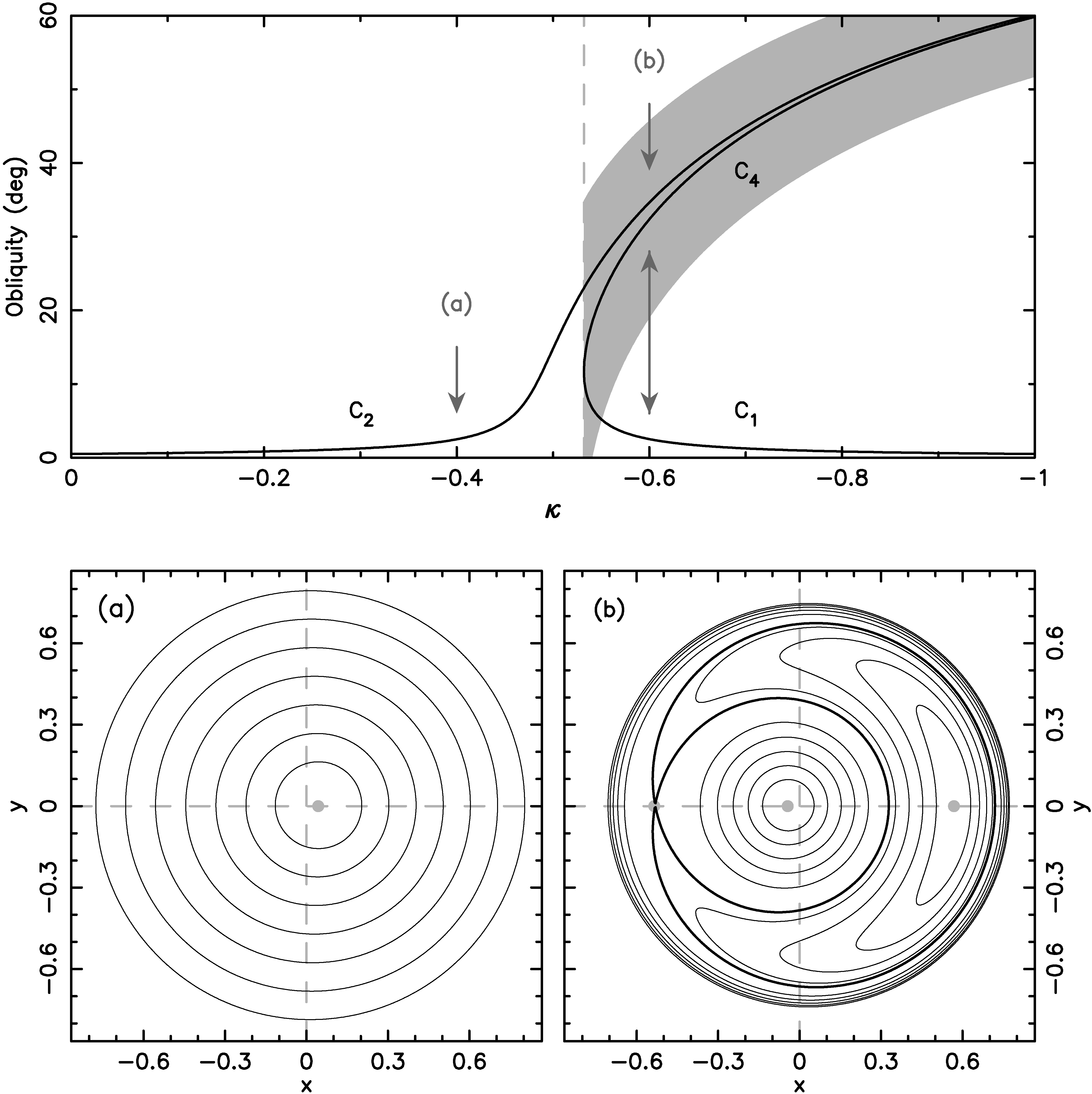
Figure 1: Top panel: Parametric dependence of Cassini state C₁, C₂ and C₄ obliquity (ordinate) on the frequency-ratio parameter $\kappa$ (abscissa) in the Colombo model (the C₃ equilibirium has obliquity larger than $90^{\circ}$ and it is not relevant for our discussion). The orbital inclination $I$ has been set to $0.5^{\circ}$ value. The dashed line indicates the critical value $-\kappa_{\star}$ at which C₁ and C₄ bifurcate (Eq. 10). The gray area for $|\kappa|>\kappa_{\star}$ shows maximum width of the resonant zone around C₂. Bottom panels: Examples of phase portraits ${\cal H}(X^{\prime},\varphi)=C$ for two values of $\kappa$: (a) $\kappa=-0.4$ on the left, and (b) $\kappa=-0.6$ on the right. We use coordinates $x=\sin\varepsilon\cos\varphi$ and $y=\sin\varepsilon\sin\varphi$ with the origin at the north pole $\varepsilon=0$. The gray symbols show location of the Cassini equilibria and the curves are isolines ${\cal H}(X^{\prime},\varphi)=C$ for suitably chosen $C$ values. The bold line in (b) is the separatrix of the resonant zone around C₂ stationary solution.

Figure 1, top panel, shows how the location of the Cassini states and the resonance width $\Delta\varepsilon$ depend on $\kappa$, which is the fundamental parameter that changes during planetary migration. For sake of this example we assumed orbital inclination $I=0.5^{\circ}$ (note that the overall structure remains similar for even smaller inclination values considered in the next section, but would be only less apparent in the Figure). The C₁ and C₄ stationary solution bifurcate when $\kappa=\kappa_{\star}$ at a non-zero critical obliquity value $\varepsilon_{\star}={\rm atan}(\tan^{1/3}I)$ (e.g., Henrard & Murigande, 1987; Ward & Hamilton, 2004). Note that $\Delta\varepsilon$ is significant in spite of a very small value of the inclination, which manifests through its dependence on a square root of $\sin 2I$ in (12). The bottom panels show examples of the phase portraits ${\cal H}(X^{\prime},\varphi)=C$ for both sub-critical $|\kappa|<\kappa_{\star}$ and super-critical $|\kappa|>\kappa_{\star}$ cases.

3 Results

We now turn our attention to the evolution of Jupiter’s and Saturn’s obliquities during planetary migration. We first discuss the orbital evolution of planets in the instability/migration simulations of NM12 (Section 3.1). We then parametrize the planetary migration before (stage 1) and after the instability (stage 2), and use it to study the effects on Jupiter’s and Saturn’s obliquities. The two stages are considered separately in Sections 3.2 and 3.3.

3.1 The orbital evolution of giant planets

NM12 reported the results of nearly $10^{4}$ numerical integrations of planetary instability, starting from hundreds of different initial configurations of planets that were obtained from previous hydrodynamical and $N$-body calculations. The initial configurations with the 3:2 Jupiter-Saturn mean motion resonance were given special attention, because Jupiter and Saturn, radially migrating in the gas disk before its dispersal, should have become trapped into their mutual 3:2 resonance (e.g., Masset & Snellgrove, 2001; Morbidelli & Crida, 2007; Pierens & Nelson, 2008). They considered cases with four, five and six initial planets, where the additional planets were placed onto resonant orbits between Saturn and the inner ice giant, or beyond the orbit of the outer ice giant. The integrations included the effects of the transplanetary planetesimal disk. NM12 experimented with different disk masses, density profiles, instability triggers, etc., in an attempt to find solutions that satisfy several constraints, such as the orbital configuration of the outer planets, survival of the terrestrial planet, and the distribution of orbits in the asteroid belt.

NM12 found the dynamical evolution in the four planet case was typically too violent if Jupiter and Saturn start in the 3:2 resonance, leading to ejection of at least one ice giant from the Solar System. Planet ejection can be avoided if the mass of the transplanetary disk of planetesimals was large ($M_{\rm disk}\gtrsim 50$ $M_{\rm Earth}$, where $M_{\rm Earth}$ is the Earth mass), but such a massive disk would lead to excessive dynamical damping (e.g., the outer planet orbits become more circular then they are in reality) and to smooth migration that violates constraints from the survival of the terrestrial planets, and the asteroid belt. Better results were obtained when the Solar System was assumed to have five giant planets initially and one ice giant, with mass comparable to that of Uranus or Neptune, was ejected into interstellar space by Jupiter (Nesvorný, 2011; Batygin et al., 2012). The best results were obtained when the ejected planet was placed into the external 3:2 or 4:3 resonances with Saturn and $M_{\rm disk}\simeq 20$ $M_{\rm Earth}$. The range of possible outcomes was rather broad in this case, indicating that the present Solar System is neither a typical nor expected result for a given initial state.

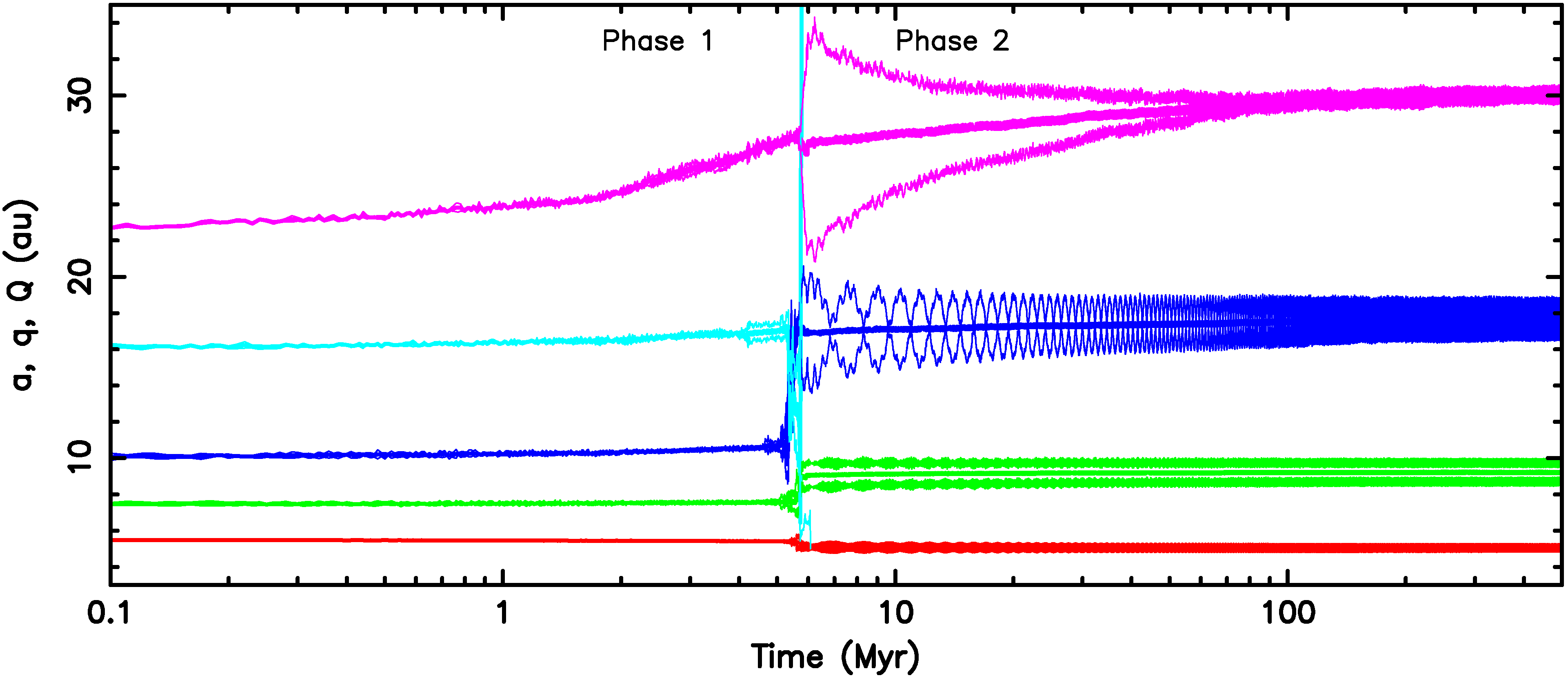
Figure 2: An example of planetary migration and instability from Nesvorný & Morbidelli (2012). The plot shows the evolution of the semimajor axis (bold line), and the perihelion and aphelion distances (thin lines) of the giant planets. The initial orbits of Jupiter, Saturn and the inner ice giant were placed in the 3:2 resonant chain. The semimajor axes of the two outer ice giants were set to be $16$ au and $22$ au. The trans-Neptunian disk of planetesimals (not shown here) was resolved by 10,000 equal-mass particles. The disk originally extended from $23.5$ au to $29$ au and had the total mass of $20$ $M_{\rm Earth}$. The instability happened at $t\simeq 5.6$ Myr after the start of the simulation. The third ice giant was subsequently ejected from the Solar system. Note that the migration rate before the instability (phase 1) is significantly larger than the migration rate after the instability (phase 2).

The most relevant feature of the NM12 models for this work is that the planetary migration happens in two stages (see Fig. 2). During the first stage, that is before the instability happens, Neptune migrates into the outer disk at $\simeq 20-30$ au. The migration is relatively fast during this stage, because the outer disk still has a relatively large mass. We analyzed several simulations from NM12 and found that Neptune’s migration can be approximately described by an exponential with the e-folding timescale $\tau\simeq 10$ Myr for $M_{\rm disk}=20$ $M_{\rm Earth}$ and $\tau\simeq 20$ Myr for $M_{\rm disk}=15$ $M_{\rm Earth}$. The instability typically happens in the NM12 models when Neptune reaches $\simeq 28$ au. The main characteristic of the instability is that planetary encounters occur, mainly between the extra ice giant and all other planets. The instability typically lasts $\sim 10^{5}$ years and terminates when the extra ice giant is ejected from the solar system by Jupiter. The second stage of migration starts after that. The migration of Neptune is much slower during this period, because the outer disk is now very much depleted. From simulations in NM12 we find that $\tau\simeq 30$ Myr for $M_{\rm disk}=20$ $M_{\rm Earth}$ and $\tau\simeq 50$ Myr for $M_{\rm disk}=15$ $M_{\rm Earth}$. Moreover, rather then being precisely exponential, the migration slows down relative to an exponential with fixed $\tau$, such as, effectively, the very late stages have larger $\tau$ values ($\tau\sim 100$ Myr) than the ones immediately following the instability. Uranus accompanies the migration of Neptune on timescales similar to those mentioned above.

The frequencies $s_{7}$ and $s_{8}$, which are the most relevant for this work, are initially somewhat higher than the precession constants of Jupiter and Saturn, mainly because of the torques from the outer disk. The extra term from the third ice giant initially located at $\simeq 10$ au has much faster frequency then the precession constants and does not interfere with the obliquity of Jupiter and Saturn during the subsequent evolution. The $s_{7}$ and $s_{8}$ frequencies slowly decrease during both stages. Their e-folding timescales may slightly differ from the migration e-folding timescales mentioned above, due to the non-linearity of the dependence of the secular frequencies on the semimajor axis of planets. Our tests show that they are about $(90-95)$% of the e-folding timescales of planetary semimajor axes.

From analyzing the behavior of frequencies in different simulations we found that $s_{8}$ should cross the value of Jupiter’s precession constant during the first migration stage, that is before the instability. The main characteristic of this crossing is that the planetary orbits are very nearly coplanar during this stage. The amplitude $I$ in Eq. (2.2) should thus be very small. It is not known exactly, however, how small. In Section 3.2, we consider amplitudes down to $0.005^{\circ}$ (about $10$ times smaller than the present value of $I_{58}$, where $I_{58}$ is the amplitude of the $8$th frequency term in Jupiter’s orbit), and show that the effects on Jupiter’s obliquity are negligible if the amplitudes were even lower. The second characteristic of the first migration stage is that the evolution of $s_{8}$ happens on a characteristic timescale of $\simeq 10-20$ Myr. Since the total change of $s_{8}$ during this interval is several arcsec yr^-1, and the first stage typically lasts $\sim 10-20$ Myr, the average rate of change is very roughly, as an order of magnitude estimate, ${\rm d}s_{8}/{\rm d}t\sim 0.1$ arcsec yr^-1 Myr^-1. The actual value of ${\rm d}s_{8}/{\rm d}t$ during crossing depends on several unknowns, including when exactly the crossing happens during the first stage. Also, the changes of $s_{8}$ could have been slower if the first stage lasted longer than in the NM12 simulations, as required if the instability occurred at the time of the Late Heavy Bombardment (e.g., Gomes et al., 2005). In Section 3.2, we will consider values in the range $0.005<{\rm d}s_{8}/{\rm d}t<0.05$ arcsec yr^-1 Myr^-1, and show that the obliquity of Jupiter cannot be pumped up to its current value if ${\rm d}s_{8}/{\rm d}t>0.05$ arcsec yr^-1 Myr^-1 (assuming that $I_{58}\lesssim 0.05^{\circ}$).

Interesting effects on obliquities should happen during the second migration stage. First, the $s_{8}$ frequency reaches the value of the precession constant of Saturn. There are several differences with respect to the $s_{8}$ crossing of Jupiter’s precession constant during the first stage (discussed above). The orbital inclinations of planets were presumably excited to their current values during the instability. Therefore, the amplitude $I_{68}$ should be comparable to its current value, $I_{68}\simeq 0.064^{\circ}$, during the second stage. We see this happening in the NM12 simulations. First, there is a brief period during the instability, when the inclinations of all planets are excited by encounters with the ejected ice giant. The inclination of Neptune is modest, at most $\simeq 2^{\circ}$, and is rather quickly damped by the planetesimal disk. Also, the invariant plane of the solar system changes by $\simeq 0.5^{\circ}$ when the third ice giant is ejected during the instability. The final inclinations are of this order. The current amplitudes are $I_{\rm 58}\simeq 0.066^{\circ}$ ($s_{8}$ term in Jupiter’s orbit) and $I_{\rm 68}\simeq 0.064^{\circ}$ ($s_{8}$ term in Saturn’s orbit) (see e.g., Laskar, 1988).

Another difference with respect the first stage is that the evolution of $s_{8}$ is much slower during the second stage. If, as indicated by the NM12 integration, $s_{8}$ changes by $\sim 1$ arcsec yr^-1 in $100$ Myr, then the average rate of change is very roughly ${\rm d}s_{8}/{\rm d}t\sim 0.01$ arcsec yr^-1 Myr^-1. The actual rate of change can be considerably lower than this during the very late times, when the effective $\tau$ was lower than during the initial stages. Finally, during the very last gasp of migration, the $s_{7}$ frequency should have approached the precession constant of Jupiter. We study this case in an adiabatic approximation when the rate of change of $s_{7}$ is much slower than any other relevant timescale. We find that the present obliquity of Jupiter can be excited by the interaction with the $s_{7}$ term only if the precession constant of Jupiter is somewhat larger than inferred by Helled et al. (2011), in accord with the results of Ward & Canup (2006).

3.2 The effects on Jupiter’s obliquity during stage 1

Since $s_{8}$ remains larger than $\alpha_{\rm S}$ during the first stage, we do not expect any important effects on Saturn’s obliquity during this stage. If Saturn’s obliquity was low initially, it should have remained low in all times before the instability. We therefore focus on the case of Jupiter in this section. From the analysis of the NM12 numerical simulation in Section 3.1, we infer that the $s_{8}$ frequency crossed $\alpha_{\rm J}$ during the first stage. The values of ${\rm d}s_{8}/{\rm d}t$ and $I_{58}$ during crossing are not known exactly from the NM12 simulations, because they depend on details of the initial conditions. We therefore consider a range of values and determine how Jupiter’s obliquity excitation depends on them. The results can be used to constrain future simulations of the planetary instability/migration.

We consider Colombo’s model with only one Fourier term in $\zeta$ of Jupiter, namely that of the $s_{8}$ frequency. The inclination term $I_{58}$ in Jupiter’s orbit was treated as a free parameter. The range of values was set to be between zero and roughly the current value of $\simeq 0.066^{\circ}$. As we discussed in Section 3.1, it is reasonable to assume that $I_{58}$ was smaller than the current value, because the orbital inclination of planets should have been low in times before the instability. The value of $\alpha_{\rm J}$ was obtained by rescaling the present value to the the semimajor axis of Jupiter before the instability ($a_{\rm J}\simeq 5.45$ au). To do so we used Eq. (2) and assumed $\alpha_{\rm J}\propto a_{\rm J}^{-3}$. No additional modeling of possible past changes of $\alpha_{\rm J}$, for instance due to satellite system evolution or planetary contraction, was implemented. The $s_{8}$ frequency was slowly decreased from a value larger than $\alpha_{\rm J}$ to a value smaller than $\alpha_{\rm J}$.

Motivated by the numerical simulations of the instability discussed in Section 3.1, we assumed the initial $s_{8}$ value of $-4$ arcsec yr^-1 and let it decrease to $-1.2$ arcsec yr^-1 by the end of each test. The rate of change, ${\rm d}s_{8}/{\rm d}t$, was treated as a free parameter. The integrations were carried for several tens of Myr for the highest assumed rates and up to several hundreds of Myr for the lowest rates. We recorded Jupiter’s obliquity during the last $5$ Myr of each run, and computed the mean value $\varepsilon_{\rm fin}$. Jupiter’s initial spin axis was oriented toward the pole of the Laplacian plane. [The value of $\varepsilon_{\rm fin}$ reported in Fig. 3 was averaged over all possible phases of the initial spin axis on the $\mathcal{H}(X^{\prime},\varphi)=C$ level curve, with $C$ defined by ${\bf s}$ oriented toward the pole of the Laplacian plane]

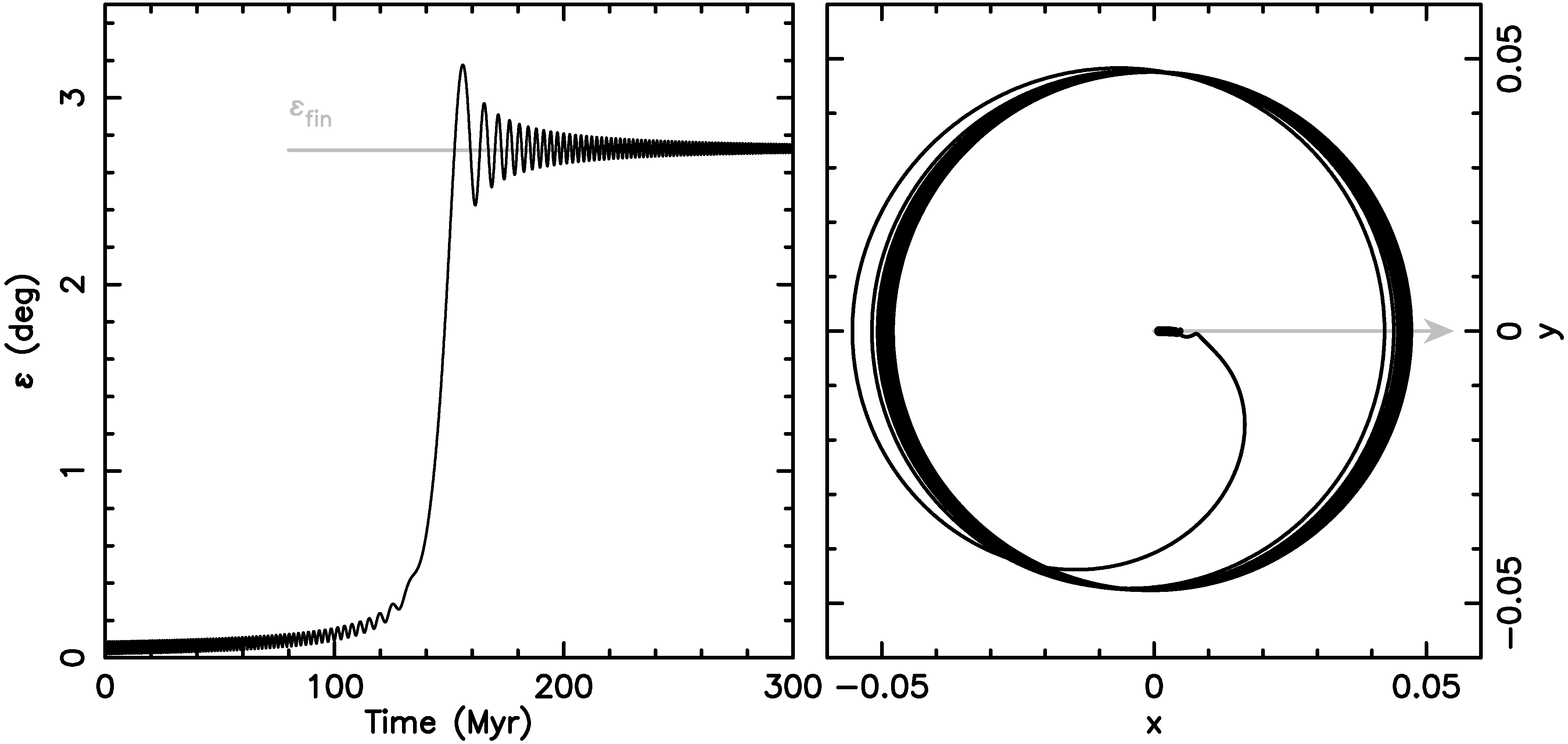
Figure 4: An example demonstrating the effect of $s_{8}$ frequency sweeping over $\alpha_{\rm J}$. Here we set $I_{58}=0.02^{\circ}$ and ${\rm d}s_{8}/{\rm d}t=0.01$ arcsec yr^-1 Myr^-1. The left panel shows Jupiter’s obliquity as a function of time. Obliquity $\varepsilon_{\rm J}$ increases to $\simeq 2.7^{\circ}$ during the resonance crossing. The width of the Cassini resonance is small because $I_{58}$ is small, and the assumed rate ${\rm d}s_{8}/{\rm d}t$ is too large in this case to lead to capture. The right panel shows the spin axis evolution projected onto the $(x,y)$ plane, where $x=\sin\varepsilon\cos\varphi$ and $y=\sin\varepsilon\sin\varphi$. The Cassini state C₂ drifts along the $x$-axis during the integration (as indicated by the gray arrow), and reaches very large obliquity values.

Figure 3 shows the results. For most parameter combinations shown here the $s_{8}$ resonance swept over $\alpha_{\rm J}$ without having the ability to capture Jupiter’s spin vector in the resonance. This happened because ${\rm d}s_{8}/{\rm d}t$ was relatively large and $I_{58}$ was relatively small, thus implying that the $s_{8}$ frequency crossed the resonant zone in a time interval that was shorter than the libration period. Captures occurred only in extreme cases (largest $I_{58}$ and smallest $ds_{8}/dt$). These cases ended up generating very large obliquity values of Jupiter and are clearly implausible. The plausible values of ${\rm d}s_{8}/{\rm d}t$ and $I_{58}$ correspond to the cases where Jupiter’s obliquity was not excited at all, thus assuming that Jupiter obtained its present obliquity later, or was excited by up to $\simeq 3^{\circ}$. To obtain $\varepsilon_{\rm J}\simeq 3^{\circ}$, ${\rm d}s_{8}/{\rm d}t$ and $I_{58}$ would need to have values along the bold line labeled 3 in Fig. 3, which extends diagonally in ${\rm d}s_{8}/{\rm d}t$ and $I_{58}$ space. An example of a case, where the obliquity of Jupiter was excited to near $\simeq 3^{\circ}$ value, is shown in Fig. 4.

3.3 Behavior of obliquities during stage 2

We now turn our attention to the second stage, when the migration slowed down and the obliquities of Jupiter and Saturn should have suffered additional perturbations. At the beginning of stage, that is just after the time of the instability, the $s_{8}$ frequency is already lower than $\alpha_{\rm J}$, but still higher than $\alpha_{\rm S}$, while the $s_{7}$ frequency is higher than $\alpha_{\rm J}$. Since the $s_{7}$ and $s_{8}$ frequencies are slowly decreasing during the second stage, a possibility arises that Jupiter’s obliquity was (slightly) excited when $s_{7}$ approached $\alpha_{\rm J}$ (e.g., Ward & Canup, 2006), and that Saturn’s obliquity was strongly excited by capture into the spin-orbit resonance with $s_{8}$ (e.g., Ward & Hamilton, 2004; Hamilton & Ward, 2004; Boué et al., 2009).

3.3.1 Jupiter

Ward & Canup (2006) suggested a possibility that Jupiter’s present obliquity may be explained by the proximity of $\alpha_{\rm J}$ to the current value of the $s_{7}$ frequency. They showed that, if $\kappa=\alpha_{\rm J}/(2s_{7})$ is sufficiently close to the critical value from Eq. (10), namely $\simeq\text@frac{1}{2}$ for small inclinations, the obliquity of the Cassini state C₂ may be significant. Thus, as $s_{7}$ adiabatically approached to $\alpha_{\rm J}$, Jupiter’s obliquity may have been excited along. As a supportive argument for this scenario they pointed out that $\varphi_{\rm J}\simeq 0^{\circ}$, where the Cassini state 2 is located.

To test this possibility we run a suite of simulations, assuming an exponential convergence to the current value $s_{7}\simeq-2.985$ arcsec yr^-1. Specifically, we set $s_{7}(t)=s_{7}(0)+[s_{7}-s_{7}(0)]\exp(-t/\tau)$, where $\tau$ and $s_{7}(0)$ are parameters. The initial value $s_{7}(0)$ at the beginning of the second stage was obtained from the numerical simulation discussed in Section 3.1. Here we chose to use $s_{7}(0)=-3.5$ arcsec yr^-1, however we verified that the results are insensitive to this choice. The e-folding timescale $\tau$ depends on how slow or fast planets migrate. Given that the planetary migration is slow during the second stage, we chose $\tau=100-200$ Myr. This assures that the approach of $s_{7}(t)$ to $\alpha_{\rm J}$ is adiabatical. The amplitude $I_{57}$ is assumed to be constant and equal to its current value ($I_{57}\simeq 0.055^{\circ}$).

Two additional parameters need to be specified: (i) Jupiter’s initial spin state, and (ii) $\alpha_{\rm J}$. As for (i), the results discussed in Section 3.2 indicate that Jupiter’s obliquity may have remained near zero during the first stage, if $I_{58}$ was too small and/or ${\rm d}s_{8}/{\rm d}t$ was too fast, or could have been potentially excited to $\simeq 3^{\circ}$, if $I_{58}$ and ${\rm d}s_{8}/{\rm d}t$ combined in the right way. Therefore, here we treat the obliquity of Jupiter at the beginning of stage 2 as a free parameter. As for (ii), as we discussed in Section 1, the present value of $\alpha_{\rm J}$ somewhat uncertain. We therefore performed various simulations, where $\alpha_{\rm J}$ takes on a number of different values between $2.75$ arcsec yr^-1 and 2.95 arcsec yr^-1. A similar approach has also been adopted by Ward & Canup (2006).

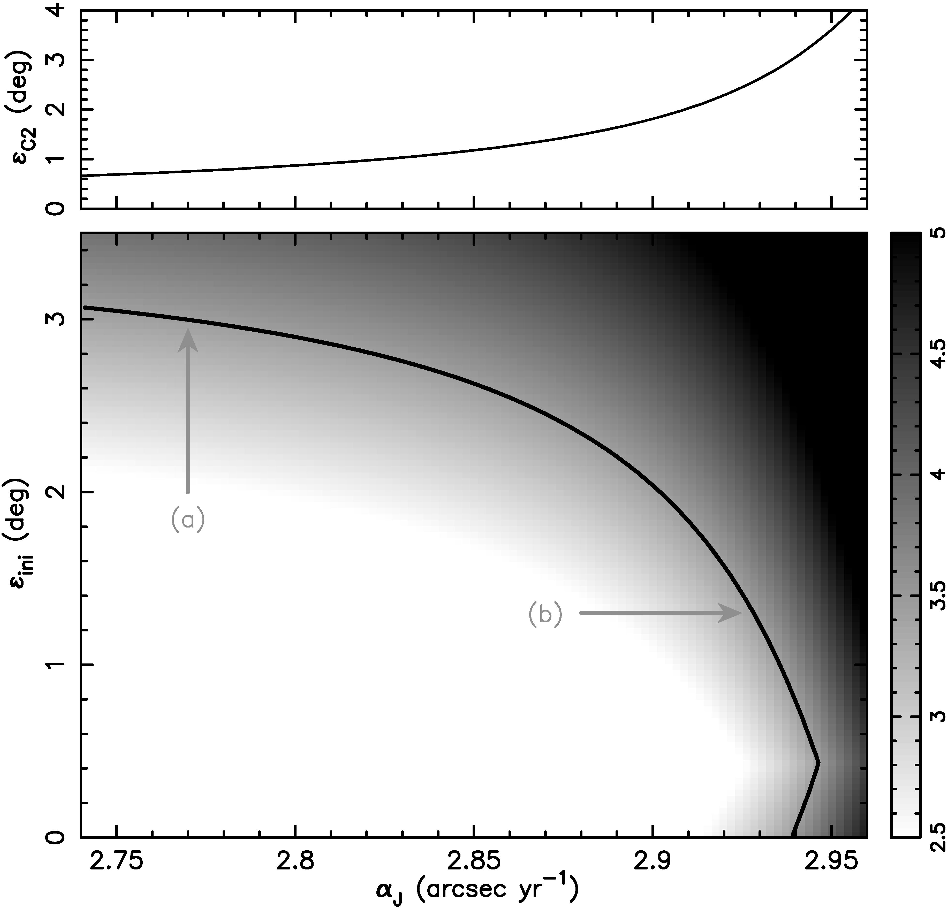
Figure 5: Final obliquity of Jupiter resulting from an adiabatic approach of the $s_{7}$-frequency towards $\alpha_{\rm J}$ (the obliquity has been computed in the reference frame associated with this frequency term in $\zeta$). While today’s value of $s_{7}$ is known fairly accurately, $\alpha_{\rm J}$ has a significant uncertainty. We therefore treat $\alpha_{\rm J}$ as a free parameter. The initial obliquity of Jupiter is also treated as a free parameter, because it depends on the effects during the first migration stage (see Fig. 3). The key to the shading scale is provided by the vertical bar on the right (white region corresponds to the final maximum obliquity smaller than $2.5^{\circ}$, incompatible with Jupiter’s value). The bold curve corresponds to the $3.45^{\circ}$ isoline, estimated obliquity value today in this frame (e.g., Ward & Canup, 2006). The arrows indicate parametric location of the two examples shown on Fig. 6. The upper panel shows the obliquity value of the Cassini state C₂ as a function of $\alpha_{\rm J}$.

Figure 5 reports the results. The top panel shows how the obliquity $\varepsilon_{\rm C2}$ of the Cassini state C₂ depends on the assumed value of $\alpha_{\rm J}$. This is calculated from Eq. (11). The trend is that $\varepsilon_{\rm C2}$ increases with $\alpha_{\rm J}$, because the larger values of $\alpha_{\rm J}$ correspond to a situation where the system is closer to the exact resonance with $s_{7}$. If $\alpha_{\rm J}<2.8$ arcsec yr^-1, as inferred from models in Helled et al. (2011), $\varepsilon_{\rm C2}$ is too small to significantly contribute to $\varepsilon_{\rm J}$. This case would imply that Jupiter’s present obliquity had to be acquired during the earlier stages and is possibly related to the non-adiabatic $s_{8}$ resonance crossing discussed in Section 3.2. If, on the other hand, $\alpha_{\rm J}\simeq 2.92-2.94$ arcsec yr^-1, Jupiter would owe its present obliquity to the proximity between $\alpha_{\rm J}$ and $s_{7}$. This would imply that the obliquity excitation during the first stage of planetary migration must have been minimal. Figures 3 and 5 express the joint constraint on the planetary migration also for the intermediate cases, where the present obliquity of Jupiter arose as a combination of both effects discussed here.

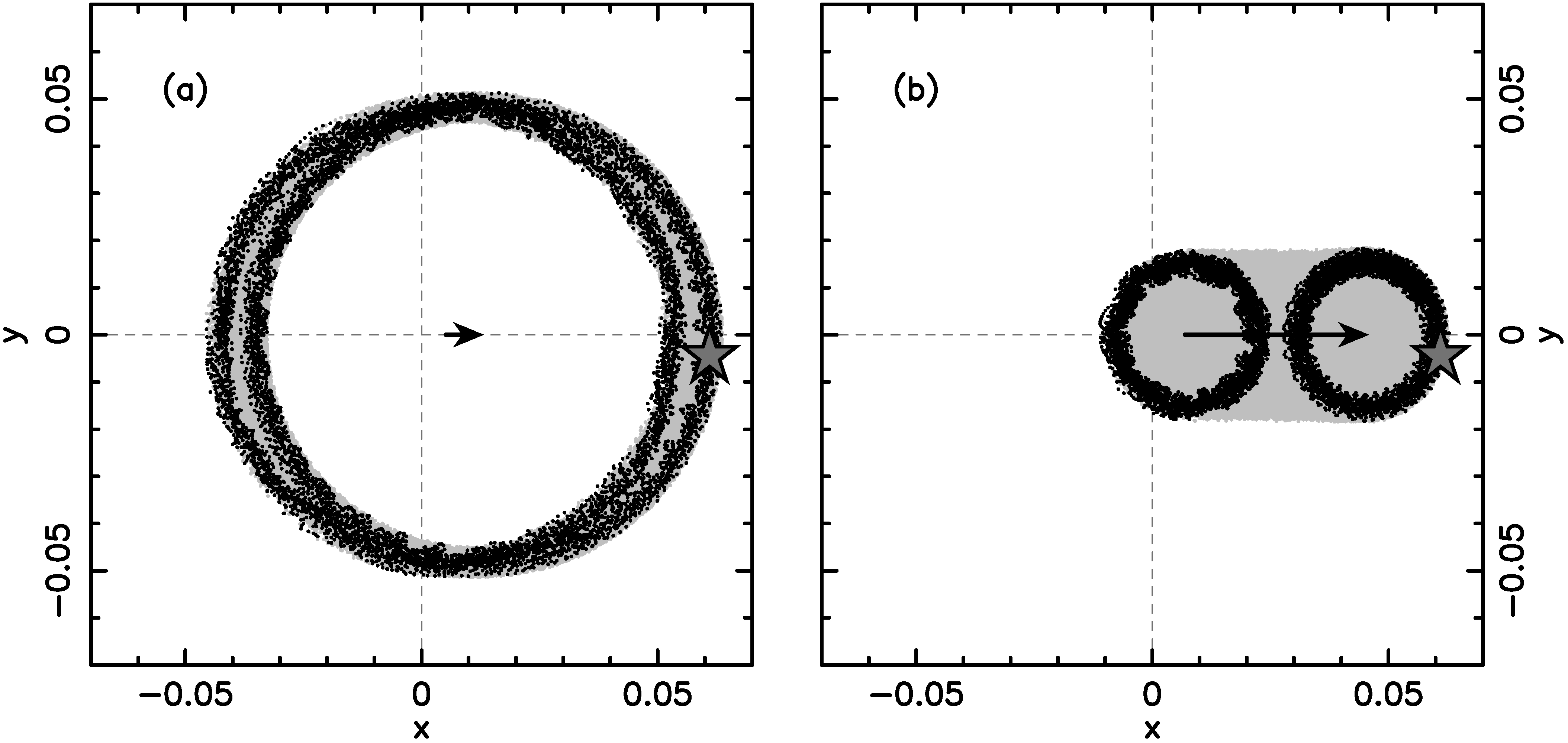
Figure 6: Two examples of Jupiter’s spin state evolution during the 1 Gyr-long time interval after the planetary instability. The planet pole is shown in the Cartesian coordinates $x=\sin\varepsilon\cos\varphi$ and $y=\sin\varepsilon\sin\varphi$. The arrow shows evolution of the Cassini state C₂ over the interval of time covered by the simulation. The gray star shows the current location of Jupiter’s pole in these coordinates. Gray dots show the pole position output every $5$ kyr during the simulation, the black circles highlight the first and the last $30$ Myr of the evolution. Two different parametric combination along the bold curve in Fig. 5 were chosen: (i) $\alpha_{\rm J}=2.77$ arcsec yr^-1 and $\varepsilon_{\rm ini}=3.1^{\circ}$ in the left panel (a), and (ii) $\alpha_{\rm J}=2.93$ arcsec yr^-1 and $\varepsilon_{\rm ini}=1.3^{\circ}$ in the right panel (b).

Figure 6 illustrates the two limiting cases discussed above. In panel (a), we assumed that the parameters during the first migration stage were such that the obliquity of Jupiter was excited to its current value during the $s_{8}$ crossing (such as shown in Fig. 4). Also, we set $\alpha_{\rm J}=2.77$ arcsec yr^-1, corresponding to the best theoretical value of Helled et al. (2011). The Cassini state C₂ corresponding to the $s_{7}$ term is only slightly displaced from the center of the plot, and does not significantly contribute to the present obliquity value. In panel (b) of Fig. 6, we set $\alpha_{\rm J}=2.93$ arcsec yr^-1. This value implies that $\varepsilon_{\rm C2}\simeq 2.6^{\circ}$. The present obliquity of Jupiter would then be in large part due to the “forced” term arising from the proximity of $s_{7}$. The initial excitation of Jupiter’s obliquity during the first stage would have to be minor in this case.

3.3.2 Saturn

In the case of Saturn, all action is expected to take place during the second stage of planetary migration. Insights gleaned from the numerical simulations discussed in Section 3.1 show that the $s_{8}$ frequency should have very slowly approached $\alpha_{\rm S}$, thus providing a conceptual basis for capture of Saturn’s spin vector in a resonance with $s_{8}$ (e.g., Ward & Hamilton, 2004; Hamilton & Ward, 2004; Boué et al., 2009). To study this possibility, we assume that the $I_{68}$ amplitude was excited to its current value during the instability, and remained nearly constant during the second stage of planetary migration. This choice is motivated by the NM12 simulations, where the inclination of Neptune is never too large. Note that Boué et al. (2009) investigated the opposite case where Neptune’s inclination was substantially excited during the instability and remained high when the resonance with $s_{8}$ occurred. This type of strong inclination excitation does not happen in the NM12 models.

Here we assume that the planetary migration was very slow during the second stage and parametrize $s_{8}(t)$ as $s_{8}(t)=s_{8}(0)+[s_{8}-s_{8}(0)]\exp(-t/\tau)$ with $\tau\geq 80$ Myr. The initial frequency value at the beginning of stage 2, $s_{8}(0)$, is estimated from the NM12 simulations. We find that $s_{8}(0)\simeq-1.3$ arcsec yr^-1, and use this value to set up the evolution of $s_{8}(t)$. We also assume a range of $\alpha_{\rm S}$ values. This has the following significance. As already pointed out by Boué et al. (2009), the best-modeling values of $\alpha_{\rm S}$ from Helled et al. (2009) are not compatible with a resonant location of Saturn’s spin axis. This is because the Cassini state C₂ would be moved to a significantly larger obliquity value ($\geq 34^{\circ}$). So these values of $\alpha_{\rm S}$ would imply that Saturn’s spin circulates about the Cassini state C₁. On the other hand, the significant obliquity of Saturn requires an increase when the $s_{8}$ value was crossing $\alpha_{\rm S}$ value, as schematically shown in the left panel of Fig. 4 for Jupiter’s obliquity during the phase 1. Boué et al. (2009) tested this scenario using numerical simulations and found it extremely unlikely: initial data of an insignificant measure have led this way to the current spin state of Saturn. Indeed, here we recover the same result with a less extensive set of numerical simulations.

Given the arguments discussed above we therefore tend to believe that the precession constant of Saturn may be somewhat smaller than the one determined by Helled et al. (2009). For instance, R. A. Jacobson (personal communication) determined the Saturn precession from the Saturn’s ring observations. The mean precession rate obtained by him is $0.725$ arcsec yr^-1 (formal uncertainty of about 6%). This value would indicate $\alpha_{\rm S}$ in the range between $0.769$ arcsec yr^-1 and $0.864$ arcsec yr^-1. Both Ward & Hamilton (2004) and Boué et al. (2009) report other observational constraints of Saturn’s pole precession that have comparably large uncertainty. We therefore sampled a larger interval of the $\alpha_{\rm S}$ values to make sure that all interesting possibilities are accounted for.

Our numerical simulations thus spanned a grid of two parameters: (i) $\alpha_{\rm S}$ discussed above, and (ii) $\tau$, the e-folding timescale of the $s_{8}$ frequency that slowly changes due to residual migration of Neptune and depletion of the outer disk. The amplitude related to the $s_{8}$ term in the inclination vector $\zeta$ of Saturn is kept constant, namely $I_{68}=0.064^{\circ}$. To keep number of tested free parameters low, we assumed initial orientation of Saturn’s spin axis ${\bf s}$ to be near the pole of the invariable plane. Specifically, we set its obliquity to $0.1^{\circ}$ in the reference frame of the $s_{8}$-frequency Fourier term in $\zeta$. To prevent fluke results, we sampled 36 values of longitude $\varphi$ of the Saturn’s pole in the same reference frame, incrementing it from $0^{\circ}$ by $10^{\circ}$. Each of the simulations covered a $1$ Gyr timespan. We recorded Saturn’s pole orientation during the last $150$ Myr time interval. We specifically analysed if it passes close to the current location of Saturn’s pole, namely $\varepsilon_{8}\simeq 27.4^{\circ}$ and $\varphi_{8}\simeq-31.4^{\circ}$ in the $s_{8}$-frequency reference frame (see Table 2 in Ward & Hamilton 2004). A numerical run was considered successful, if the simulated Saturn’s pole passed through a box of $\pm 0.2^{\circ}$ in obliquity $\varepsilon$ and $\pm 3^{\circ}$ in longitude $\varphi$ around the planet’s values $(\varepsilon_{8},\varphi_{8})$ during the recorded $150$ Myr time interval. Note that the libration period of Saturn’s pole around Cassini state C₂, if captured in the spin-orbit resonance, is $\sim(50-100)$ Myr, depending on the libration amplitude. This set our requirement for the timespan over which we monitored Saturn’s pole position.

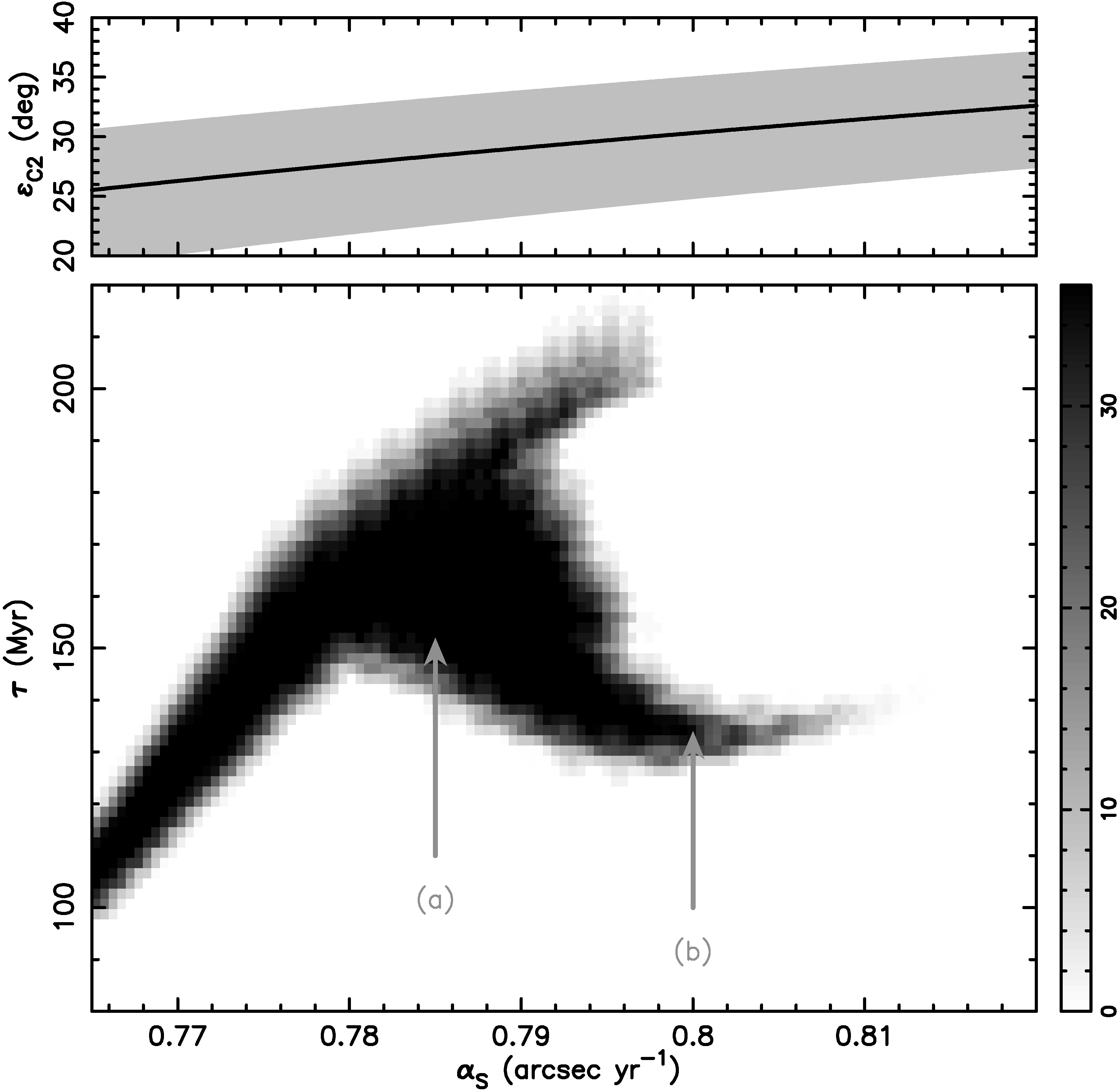
Figure 7: Bottom panel: Distribution of solutions successfully matching Saturn’s spin state in the parametric plane $\alpha_{\rm S}$ (abscissa) vs $\tau$ (ordinate), the e-folding time of $s_{8}$-frequency evolution during the phase 2. No successful solutions were obtained in the white region of the plot. The darker the gray-scale in the given bin, the more robust the solution is. The maximum value 36 corresponds to 36 sampled initial conditions of the simulations for each $(\alpha_{\rm S},\tau)$ pair (see the side bar). When $\alpha_{\rm S}\simeq 0.78$ arcsec yr^-1, the obliquity of the corresponding to Cassini state C₂ is $\simeq 27.4^{\circ}$. Therefore the capture solution corresponds to the minimum needed libration amplitude of Saturn’s spin in the $s_{8}$ reference frame. From this value the larger libration-amplitude solutions bifurcate towards smaller/larger $\alpha_{\rm S}$ values. The arrows indicate parametric location of two particular examples shown on panels (a) and (b) of Fig. 8. Top panel: Obliquity of the Cassini state C₂ (solid line) and maximum width of the associated resonant zone (gray area) as a function of $\alpha_{\rm S}$. We assume inclination $I=I_{68}=0.064^{\circ}$ and terminal value of the orbital precession frequency $s_{8}\simeq-0.692$ arcsec yr^-1.

Figure 7 shows the results from this suite of runs. The shaded region shows correlated $\alpha_{\rm S}$-$\tau$ pairs that provided successful match to the Saturn’s pole position. We note that no successful solutions were obtained for $\alpha_{\rm S}>0.812$ arcsec yr^-1 and all successful solutions correspond to the capture in the resonance zone around the Cassini state C₂. The absence of low-probability solutions in which Saturn’s pole would circulate about the Cassini state C₁ for larger $\alpha_{\rm S}$ may be related to the limited number of simulations performed. No solutions were also obtained for $\tau>215$ Myr. This is because for such long e-folding timescales the resonant capture process would be strictly adiabatic and the simulated spin would not meet the condition of at least $30^{\circ}$ libration amplitude (see discussion in Ward & Hamilton, 2004; Hamilton & Ward, 2004). The area occupied by successful solutions splits into two branches for $\alpha_{\rm S}\simeq 0.78$ arcsec yr^-1. This is because the obliquity of the Cassini state C₂ is $\varepsilon_{\rm C2}\simeq 27.4^{\circ}$ for the critical value of $\alpha_{\rm S}$, and the solutions have the minimum libration amplitude of $\simeq 31^{\circ}$.

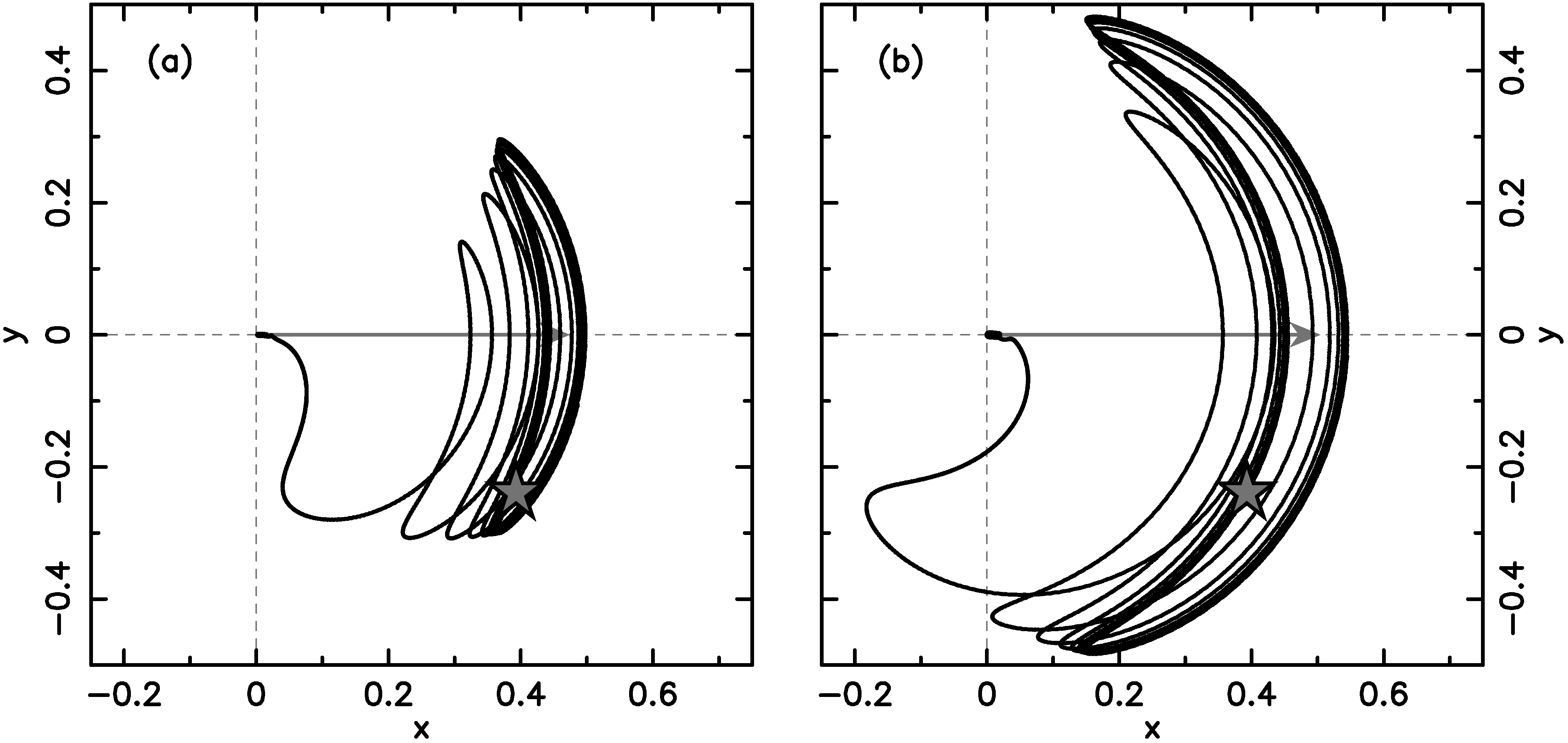
Figure 8: Two examples Saturn’s obliquity excitation by the capture and evolution in the resonance with $s_{8}$. The spin axis ${\bf s}$ is projected onto the $(x,y)$ plane, where $x=\sin\varepsilon\cos\varphi$ and $y=\sin\varepsilon\sin\varphi$. The reference frame used here is the one associated with the $s_{8}$ frequency term contributing to $\zeta$ of Saturn. The gray arrow shows the evolution of the Cassini state C₂ over the full length of the simulation ($1$ Gyr). In panel (a), we assumed that $\alpha_{\rm S}=0.785$ arcsec yr^-1, which means that the terminal obliquity of C₂ is at $\simeq 28.2^{\circ}$, and $\tau=150$ Myr. In (b), we used $\alpha_{\rm S}=0.8$ arcsec yr^-1, which means that the terminal obliquity of C₂ is at $\simeq 30.3^{\circ}$, and $\tau=135$ My. These combinations were also highlighted by arrows on Fig. 7. The star in each panel shows the present orientation of the Saturn pole vector in the $(x,y)$ coordinates (e.g., Ward & Hamilton, 2004, Table 2).

Figure 8 shows two evolution paths of Saturn’s spin vector obtained in two different simulations. As mentioned above, in both cases Saturn’s spin state was captured into the spin-orbit resonance $s_{8}$, and remained in the resonance for the full length of the simulation. The final states of both simulations are a good proxy for the Saturn’s present spin state. These two cases differ from each other principally because the path in panel (b) shows librations with a larger amplitude than the path in panel (a). Note some of the solutions, such as (b) here, may attain a significant librations amplitude. This is because with the corresponding values of $\tau\simeq 100$ Myr the evolution is not adiabatic and the librations amplitude is excited immediately after capture. Therefore, the complicated evolution histories proposed in Hamilton & Ward (2004) may not be needed.

4 Conclusions

We studied the behavior of Jupiter’s and Saturn’s obliquities in models of planetary instability and migration that were informed from NM12. Rather then investigating a few specific cases directly from NM12, we considered the general concept of a two-stage migration from NM12, and studied a broad range of relevant parameter values. We found that, in general, the two stage migration provides the right framework for an adequate excitation of Jupiter’s and Saturn’s obliquities. Moreover, we found that certain conditions must be satisfied during the first and second stages of migration, if the final obliquity values are to match the present obliquities of these planets.

Our results indicate that Jupiter spin axis could have been tilted either when (i) the $s_{8}$ frequency swept over $\alpha_{\rm J}$ during the first migration stage (that is before the instability happened), or when (ii) the $s_{7}$ frequency approached $\alpha_{\rm J}$ at the end of planetary migration. For (i) to work, the crossing of $s_{8}$ must be fast, such that the capture into the resonance does not happen, but not too fast, such that some excitation is generated by the resonance crossing. To obtain full $\varepsilon_{\rm J}=3.1^{\circ}$ during this stage, the rate of change of $s_{8}$ during crossing, ${\rm d}s_{8}/{\rm d}t$, must be smaller than $0.05$ arcsec yr^-1 Myr^-1 (assuming that $I_{58}<0.05^{\circ}$). Since the evolution of $s_{8}$ mainly relates to the radial migration of Neptune and dispersal of the outer disk of planetesimals, this result implies that both these processes would need to occur relatively slowly. More specifically, parameters ${\rm d}s_{8}/{\rm d}t$ and $I_{58}$ would have to have values along a diagonal line in the (${\rm d}s_{8}/{\rm d}t$, $I_{58}$) plane with larger values of $I_{58}$ requiring larger values of ${\rm d}s_{8}/{\rm d}t$ (see Fig. 3). Any model of planetary instability/migration can be tested against this constraint. The models where ${\rm d}s_{8}/{\rm d}t$ is too slow and/or $I_{58}$ is too large, as specified in Fig. 3, can be ruled out, because Jupiter’s obliquity would be excited too much by the $s_{8}$ crossing.

Not much excitation of $\varepsilon_{\rm J}$ is expected during the $s_{8}$ crossing if ${\rm d}s_{8}/{\rm d}t$ was relatively fast and/or if $I_{58}$ was only a very small fraction of its current value. If that is the case, Jupiter’s obliquity would probably need to be excited during the very last stages of migration by (ii). For that to work, Jupiter’s precession constant $\alpha_{\rm J}$ would need to be $\simeq 2.95$ arcsec yr^-1 (assuming $\varepsilon_{\rm J}=0$ initially), which is a value that is significantly larger than the one estimated by Helled et al. (2011). This means that Helled’s model would need to be adjusted to fit within this picture. It is also possible, however, that Jupiter’s present obliquity was contributed partly by (i) and partly by (ii). If so, Figs. 3 and 5 express the joint constraint on ${\rm d}s_{8}/{\rm d}t$ and $I_{58}$ during the first stage, and $\alpha_{\rm J}$.

As for Saturn, our results indicate that the capture into the spin-orbit resonance with $s_{8}$ (Ward & Hamilton, 2004; Hamilton & Ward, 2004) is indeed possible during the late stages of planetary migration, assuming that the migration rate was slow enough. The exact constraint on the slowness of migration depends on $I_{68}$, which in turn depends how much Neptune’s inclination was excited by the instability and how long it remained elevated (Boué et al., 2009). Since in the NM12 models, Neptune’s orbital inclination is never large, we have good reasons to believe that $I_{68}$ was comparable to its current value when the crossing of $s_{8}$ occurred. Thus, using $I_{68}\simeq 0.064^{\circ}$, we find that the e-folding migration timescale $\tau$ would need to be $\tau\gtrsim 100$ Myr. If $\tau>200$ Myr, however, the capture in the $s_{8}$ resonance would be strictly adiabatic. This would imply, if $\varepsilon_{\rm S}$ was negligible before capture, that the resonant state should have a very small libration amplitude (see Ward & Hamilton, 2004; Hamilton & Ward, 2004). It would then be difficult to explain the current orientation of Saturn’s spin axis, which indicates that the libration amplitude should be at least $30^{\circ}$. A more satisfactory solution, however, can be obtained for $\tau\simeq 100-150$ Myr, in which case the capture into the resonance was not strictly adiabatic. In this case the $\geq 30^{\circ}$ libration amplitude is obtained during capture.

While the capture conditions pose a strong constraint on the timescale of Neptune’s radial migration, as discussed above, and additional constraint on Saturn’s precession constant $\alpha_{\rm S}$ derives from the present obliquity of Saturn. This is because, again assuming that Saturn spin vector is in the resonance with $s_{8}$ today, the present obliquity of Saturn implies that the Cassini state C₂ of this resonance would have to be located at $\varepsilon\sim(28-30)^{\circ}$. This would require that $\alpha_{\rm S}\simeq 0.78-0.80$ arcsec yr^-1. The value derived by Helled et al. (2009) is larger, $\simeq 0.8445$ arcsec yr^-1, and clearly incompatible with this assumption. Direct measurements of the mean precession rate of Saturn’s spin axis suggest that $\alpha_{S}\simeq 0.81$ arcsec yr^-1, which is still slightly larger than the range given above, but the uncertainty interval of this estimate includes values below $0.8$ arcsec yr^-1 (R. A. Jacobson, personal communication). Figuring out the exact value of Saturn’s precession constant will therefore be important. Once $\alpha_{\rm S}$ is known, Fig. 7 could be used to precisely constrain the timescale of planetary migration.

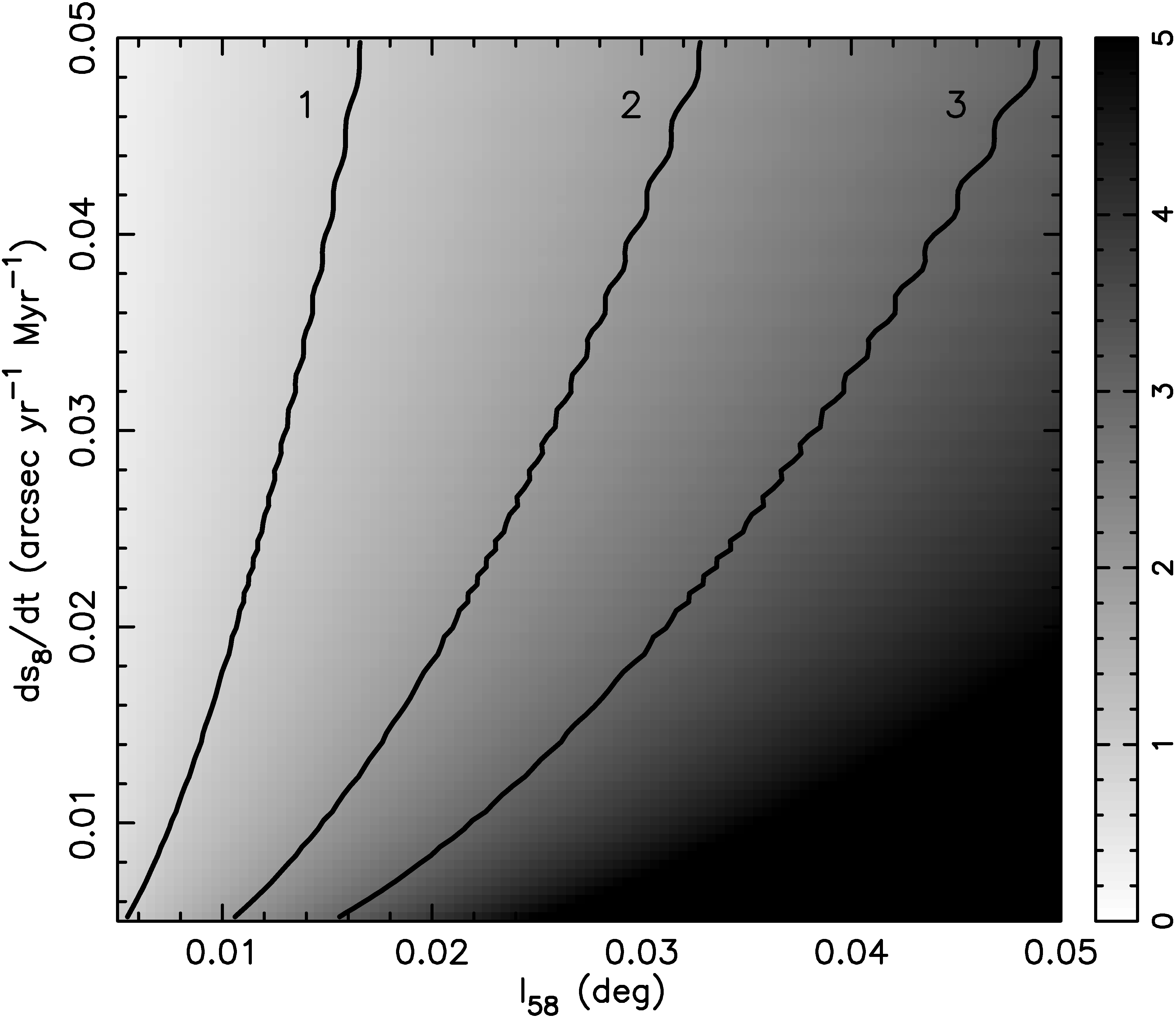
Figure 3: The final obliquity $\varepsilon_{\rm fin}$ of Jupiter obtained in our integrations of crossing of the $s_{8}$ spin-orbit resonance. Jupiter’s obliquity is shown as a function of two parameters: (i) the amplitude $I_{58}$ of the Fourier term in Jupiter’s $\zeta$ variable (see Section 2), and (ii) the rate ${\rm d}s_{8}/{\rm d}t$ at the time when $s_{8}$ became equal to $\alpha_{\rm J}$. The gray shading indicates the final obliquity (the scale bar on the right shows the corresponding numerical value in degrees). The three bold isolines correspond to $\varepsilon_{\rm J}=1^{\circ}$, $2^{\circ}$ and $3^{\circ}$ (see the labels).

References

- Applegate et al. (1986) Applegate, J. H., Douglas, M. R., Gürsel, Y., Sussman, G. J., & Wisdom, J. 1986, AJ, 92, 176
- Batygin et al. (2012) Batygin, K., Brown, M. E., & Betts, H. 2012, ApJ, 744, L3
- Brasser & Lee (2015) Brasser, R., & Lee, M. H. 2015, AJ, submitted
- Breiter et al. (2005) Breiter, S., Nesvorný, D., & Vokrouhlický, D. 2005, AJ, 130, 1267
- Brouwer & Clemence (1961) Brouwer, D., & Clemence, D. M. 1961, Methods of Celestial Mechanics, Academic Press, New York
- Boué et al. (2009) Boué, G., Laskar, J., & Kuchynka, P. 2009, ApJ, 702, L19
- Colombo (1966) Colombo, G. 1966, AJ, 71, 891
- Gomes et al. (2005) Gomes, R., Levison, H. F., Tsiganis, K., & Morbidelli, A. 2005, Nature, 435, 466
- Hamilton & Ward (2004) Hamilton, D. P., & Ward, W. R. 2004, AJ, 128, 2510
- Helled et al. (2009) Helled, R., Schubert, G., & Anderson, J. D. 2009, Icarus, 199, 368
- Helled et al. (2011) Helled, R., Anderson, J. D., Schubert, G., & Stevenson, D. J. 2011, Icarus, 216, 440
- Henrard & Murigande (1987) Henrard, J., & Murigande, C. 1987, Celestial Mechanics, 40, 345
- Laskar (1988) Laskar, J. 1988, A&A, 198, 341
- Laskar & Robutel (1993) Laskar, J., & Robutel, P. 1993, Nature, 361, 608
- Le Maistre et al. (2014) Le Maistre, S., Folkner, W. M., & Jacobson, R. A. 2014, presented at 46th DPS meeting, abstract 422.08
- Levison et al. (2008) Levison, H. F., Morbidelli, A., Van Laerhoven, C., Gomes, R., & Tsiganis, K. 2008, Icarus, 196, 258
- Lissauer & Safronov (1991) Lissauer, J. J., & Safronov, V. S. 1991, Icarus, 93, 288
- Malhotra (1995) Malhotra, R. 1995, AJ, 110, 420
- Masset & Snellgrove (2001) Masset, F., & Snellgrove, M. 2001, MNRAS, 320, L55
- McNeil & Lee (2010) McNeil, D. S., & Lee, M. H. 2010, Bull. Am. Astron. Soc., 42, 948
- Minton & Malhotra (2009) Minton, D. A., & Malhotra, R. 2009, Nature, 457, 1109
- Minton & Malhotra (2011) Minton, D. A., & Malhotra, R. 2011, ApJ, 732, 53
- Morbidelli & Crida (2007) Morbidelli, A., & Crida, S. 2007, Icarus, 191, 158
- Morbidelli et al. (2005) Morbidelli, A., Levison, H. F., Tsiganis, K., & Gomes, R. 2005, Nature, 435, 462
- Morbidelli et al. (2009) Morbidelli, A., Brasser, R., Tsiganis, K., Gomes, R., & Levison, H. F. 2009, A&A, 507, 1041
- Morbidelli et al. (2010) Morbidelli, A., Brasser, R., Gomes, R., Levison, H. F., & Tsiganis, K. 2010, AJ, 140, 1391
- Morbidelli et al. (2012) Morbidelli, A., Tsiganis, K., Batygin, K., Crida, A., & Gomes, R. 2012, Icarus, 219, 737
- Morbidelli et al. (2014) Morbidelli, A., Gaspar, H. S., & Nesvorný, D. 2014, Icarus, 232, 81
- Nesvorný (2011) Nesvorný, D. 2011, ApJ, 742, L22
- Nesvorný (2015) Nesvorný, D. 2015, AJ, submitted
- Nesvorný & Vokrouhlický (2009) Nesvorný, D., & Vokrouhlický, D. 2009, AJ, 137, 5003
- Nesvorný & Morbidelli (2012) Nesvorný, D., & Morbidelli, A. 2012, AJ, 144, 117
- Nesvorný et al. (2007) Nesvorný, D., Vokrouhlický, D., & Morbidelli, A. 2007, AJ, 133, 1962
- Nesvorný et al. (2014a) Nesvorný, D., Vokrouhlický, D., & Morbidelli, A. 2014a, ApJ, 768, 45
- Nesvorný et al. (2014b) Nesvorný, D., Vokrouhlický, D., & Deienno, R. 2014b, ApJ, 784, 22
- Pierens & Nelson (2008) Pierens, A., & Nelson, R. P. 2008, A&A, 482, 333
- Thommes et al. (1999) Thommes, E. W., Duncan, M. J., & Levison, H. F. 1999, Nature, 402, 635
- Tsiganis et al. (2005) Tsiganis, K., Gomes, R., Morbidelli, A., & Levison, H. F. 2005, Nature, 435, 459
- Ward & Hamilton (2004) Ward, W. R., & Hamilton, D. P. 2004, AJ, 128, 2501
- Ward & Canup (2006) Ward, W. R., & Canup, R. M. 2006, ApJ, 640, L91