Notes on Conservation Laws, Equations of Motion of Matter and Particle Fields in Lorentzian and Teleparallel de Sitter Spacetime Structures

Abstract

In this paper we discuss the physics of interacting tensor fields and particles living in a de Sitter manifold $M=\mathrm{S0}(1,4)/\mathrm{S0}(1,3)\simeq\mathbb{R}\times S^{3}$ interpreted as a submanifold of $(\mathring{M}=\mathbb{R}^{5},\boldsymbol{\mathring{g}})$, with $\boldsymbol{\mathring{g}}$ a metric of signature $(1,4)$. The pair $(M,\boldsymbol{g})$  where $\boldsymbol{g}$ is the pullback metric of $\boldsymbol{\mathring{g}}$ $(\boldsymbol{g=i}^{\ast}\boldsymbol{\mathring{g}})$ is a Lorentzian manifold that is oriented by $\tau_{\boldsymbol{g}}$ and time oriented by $\uparrow$. It is the structure $(M,\boldsymbol{g,}\tau_{\boldsymbol{g}},\uparrow)$ that is primely used to study the energy-momentum conservation law for a system of physical fields (and particles) living in $M$ and to get the equations of motion of the fields and also the equations of motion describing the behavior of free particles. To achieve our objectives we construct two different de Sitter spacetime structures $M^{dSL}=(M,\boldsymbol{g,D},\tau_{\boldsymbol{g}},\uparrow)$ and $M^{dSTP}=(M,\boldsymbol{g,\nabla},\tau_{\boldsymbol{g}},\uparrow)$, where $\boldsymbol{D}$ is the Levi-Civita connection of $\boldsymbol{g}$ and $\boldsymbol{\nabla}$ is a metric compatible parallel connection. Both connections are introduced in our study only as mathematical devices, no special physical meaning is attributed to these objects. In particular $M^{dSL}$ is not supposed to be the model of any gravitational field in the General Relativity Theory (GRT). Our approach permit to clarify some misconceptions appearing in the literature, in particular one claiming that free particles in the de Sitter structure $(M,\boldsymbol{g})$ do not follows timelike geodesics. The paper makes use of the Clifford and spin-Clifford bundles formalism recalled in one of the appendices, something needed for a thoughtful presentation of the concept of a Komar current $\boldsymbol{J}_{A}$ (in GRT) associated to any vector field $\mathbf{A}$ generating a one parameter group of diffeomorphisms. The explicit formula for $\boldsymbol{J}_{\emph{A}}$ in terms of the energy-momentum tensor of the fields and its physical meaning is given. Besides that we show how $F=dA$ ($A=\boldsymbol{g}(\mathbf{A},~{})$ satisfy a Maxwell like equation $\boldsymbol{\partial}F=\boldsymbol{J}_{\emph{A}}$ which encodes the contents of Einstein equation. Our results shows that in GRT there are infinitely many conserved currents, independently of the fact that the Lorentzian spacetime (representing a gravitational field) possess or not Killing vector fields. Moreover our results also show that even when the appropriate timelike and spacelike Killing vector fields exist it is not possible to define a conserved energy-momentum covector (not covector field) as in Special Relativistic Theories.

1 Introduction

In this paper we study some aspects of Physics of fields living and interacting in a manifold $M=\mathrm{SO}(1,4)\mathrm{/SO}(1,3)\simeq\mathbb{R}^{3}\times S^{3}$. We introduce two different geometrical spacetime structures that we can form starting from the manifold $M$ which is supposed to be a vector manifold, i.e., a submanifold of ($\mathring{M},\boldsymbol{\mathring{g}})$ with $\mathring{M}=\mathbb{R}^{5}$ and $\boldsymbol{\mathring{g}}$ a metric of signature $(1,4)$. If $\boldsymbol{i}:M\rightarrow\mathring{M}$ is the inclusion map the structures that will be studied are the Lorentzian de Sitter spacetime $M^{dSL}=(M,\boldsymbol{g},\boldsymbol{D},\tau_{\boldsymbol{g}},\uparrow)$ and teleparallel de Sitter spacetime $M^{dSTP}=(M,\boldsymbol{g},\boldsymbol{\nabla},\tau_{\boldsymbol{g}},\uparrow)$ where $\boldsymbol{g=i}^{\ast}\boldsymbol{\mathring{g}}$, $\boldsymbol{D}$ is the Levi-Civita connection of $\boldsymbol{g}$ and $\boldsymbol{\nabla}$ is a metric compatible teleparallel connection (see Section 4.1). Our main objective is the following: taking $(M,\boldsymbol{g})$ as the arena where physical fields live and interact how do we formulate conservation laws of energy-momentum and angular momentum for the system of physical fields. In order to give a meaningful meaning to this question we recall the fact that in Lorentzian spacetime structures that are models of gravitational fields in the GRT there are no genuine conservation laws of energy-momentum (and also angular momentum) for a closed system of fields and moreover there are no genuine energy-momentum and angular momentum conservation laws for the system consisting of non gravitational plus the gravitational field. We discuss in Section 2.1 a pure mathematical result, namely when there exists some conserved currents $\mathcal{J}_{V}$ $\in\sec T^{\ast}M$ in a Lorentzian spacetime associated to a tensor field $\boldsymbol{W\in}\sec T_{1}^{1}M$ and a vector field $\boldsymbol{V}\in\sec TM$. In Section 2.2 we briefly recall how a conserved energy-momentum tensor for the matter fields is constructed in Special Relativity theories and how in that theory it is possible to construct a conserved energy-momentum covector for the matter fields. After that we recall that in GRT we have a covariantly “conserved” energy-momentum tensor $\boldsymbol{T\in}\sec T_{1}^{1}M$ (i.e., $\boldsymbol{D\bullet T}=0$) and so, using the results of Section 2.1 we can immediately construct conserved currents when the Lorentzian spacetime modelling the gravitational field generated by $\boldsymbol{T}$ possess Killing vector fields. However, we show that is not possible in general in GRT even when some special conserved currents exist (associated to one timelike and three spacelike Killing vector fields) to build a conserved covector for the system of fields, as it is the case in special relativistic theories. Immediately after showing that we ask the question:

Is it necessary to have Killing vector fields in a Lorentzian spacetime modelling a given gravitational field in order to be possible to construct conserved currents?

Well, we show that the answer is no. In GRT there are an infinite number of conserved currents. This is showed in Section 2.4 were we introduce the so called Komar currents in a Lorentzian spacetime modelling a gravitational field generated by a given (symmetric) energy momentum tensor $\boldsymbol{T}$ and show how any diffeomorphism associated to a one parameter group generated by a vector field $\mathbf{A}$ lead to a conserved current. We show moreover using the Clifford bundle formalism recalled in Appendix A that $F=dA$ $\boldsymbol{\in}\sec{\textstyle\bigwedge\nolimits^{2}}T^{\ast}M$ where $A=\boldsymbol{g}(\mathbf{A},~{})\in\sec{\textstyle\bigwedge\nolimits^{1}}T^{\ast}M$ satisfy, (with $\boldsymbol{\partial}$ denoting the Dirac operator acting on sections of the Clifford bundle of differential forms)  a Maxwell like equation $\boldsymbol{\partial}F=\boldsymbol{J}_{A}$ (equivalent to $dF=0$ and $\underset{\boldsymbol{g}}{\delta}F=-\boldsymbol{J}_{A}$). The explicit form of $\mathcal{J}_{A}$ as a function of the energy-momentum tensor is derived  (see Eq.(48)) together with its scalar invariant. We establish that $\boldsymbol{\partial}F=\boldsymbol{J}_{A}$ encode the contents of Einstein equation. We show moreover that even if we can get four conserved currents given one time like and three spacelike vector fields and thus get four scalar invariants these objects cannot be associated to the components of a momentum covector for the system of fields producing the energy-momentum tensor $\boldsymbol{T}$. We also give the form of $\boldsymbol{J}_{A}$ when $\mathbf{A}$ is a Killing vector field and emphasize that even if the Lorentzian spacetime under consideration has one time like and three spacelike Killing vector fields we cannot find a conserved momentum covector for the system of fields.

This paper has several appendices necessary for a perfect intelligibility of the results in the main text. Thus it is opportune to describe what is there and where their contents are used in the main text. To start, in Appendix A we briefly recall the main results of the Clifford bundle formalism used in this paper which permits one to understand how to arrive at the equation $\boldsymbol{\partial}F\boldsymbol{=J}_{A}$ in Section 2.2.. Lie derivatives and variations of tensor fields is discussed in Appendix B. In Section C1 we derive from the Lagrangian formalism conserved currents for fields living in a general Lorentzian spacetime structure and the corresponding generalized covariant energy-momentum “conservation” law. We compare these results in Section C2 with the analogues ones for field theories in special relativistic theories where the Lorentzian spacetime structure is Minkowski spacetime. We show that despite the fact that we can derive conserved quantities for fields living and interacting in $M^{\ell DS}$ we cannot define in this structure a genuine energy-momentum conserved covector for the system of fields as it is the case in Minkowski spacetime. A legitimate energy-momentum covector for the system of fields living in $(M=\mathrm{SO}(1,4)\mathrm{/SO}(1,3),\boldsymbol{g})$ exist only in the teleparallel structure $M^{dSTP}$. This is discussed in Section 5.2 after recalling the Lie algebra and the Casimir invariants of the Lie algebra of de Sitter group in Section 5.1. In Appendix E we derive for completeness and to insert the Remark 32 the so called covariant energy-momentum conservation law in GRT. Appendix D recalls the intrinsic definition of relative tensors and their covariant derivatives. Appendix E present proofs of some identities used in the main text.

As we already said the main objective of this paper is to discuss the Physics of interacting fields in de Sitter spacetime structures $M^{dSL}$ and $M^{dSTP}$. In particular we want also to clarify some misunderstandings concerning the roles of geodesics in the $M^{dS\ell}$. So, in section 3 we briefly recall the conformal representation of the de Sitter spacetime structure $M^{dSL}$ and prove that the one timelike and the three spacelike “translation” Killing vector fields of $(M,\boldsymbol{g})$ defines a basis for almost all $M$. With this result we show in Section 4 that the method using in [32] to obtain the curves which extremizes the length function of timelike curves in de Sitter spacetime with the result that these curves are not geodesics is equivocated, since those authors use constrained variations instead of arbitrary variations of the length function. Even more, the equation obtained from the constrained variation in [32] is according to our view wrongly interpreted in its mathematical (and physical) contents. Indeed, using some of the results of Section 5.2 and the results of Section 6 which briefly recall Papapetrou’s classical results [29] deriving the equation of motion of a probe single-pole particle in GRT, we show in Section 7 that contrary to the authors statement in [32] it is not true that the equation of motion of a single-pole obtained from a method similar to Papapetrou’s one in [29] but using the generalized energy-momentum tensor of matter fields in $M^{dSL}$ gives an equation of motion different from the geodesic equation in $M^{dSL}$ and in agreement with the one they derived from his constrained variation method. Indeed, we prove that from the equation describing the motion of a single-pole the geodesic equation follows automatically. Finally, in Section 8 we present our conclusions.

2 Preliminaries

Let $(M,\boldsymbol{g},D,\tau_{\boldsymbol{g}},\uparrow)$ be a general Lorentzian spacetime. Let $\mathcal{U}\subseteq M$ be an open set covered by coordinates $\{x^{\mu}\}$. Let $\{e_{\mu}=\partial_{\mu}\}$ be a basis of $T\mathcal{U}$ and $\{\boldsymbol{\vartheta}^{\mu}=dx^{\mu}\}$  the basis of $T^{\ast}\mathcal{U}$ dual to the basis $\{\partial_{\mu}\}$, i.e., $\boldsymbol{\vartheta}^{\mu}(\partial_{\nu})=\delta_{\nu}^{\mu}$. We denote by $\mathtt{g}$ a metric of the cotangent bundle such that if $\boldsymbol{g}=g_{\mu\nu}\boldsymbol{\vartheta}^{\mu}\otimes\boldsymbol{\vartheta}^{\nu}$ then $\mathtt{g}=g^{\mu\nu}\partial_{\mu}\otimes\partial_{\nu}$ with $g^{\mu\rho}g_{\rho\nu}=\delta_{\nu}^{\mu}$. We introduce also $\{\partial^{\mu}\}$ and $\{\boldsymbol{\vartheta}_{\mu}\}$ respectively as the reciprocal bases of $\{e_{\mu}\}$ and $\{\boldsymbol{\vartheta}^{\mu}\}$, i.e., we have

$$\boldsymbol{g}(\partial_{\nu},\partial^{\mu})=\delta_{\nu}^{\mu},~{}~{}~{}\mathtt{g}(\boldsymbol{\vartheta}^{\mu},\boldsymbol{\vartheta}_{\nu})=\delta_{\nu}^{\mu}$$ (1)

Next we introduce in $T\mathcal{U}$ the tetrad basis $\{\boldsymbol{e}_{\alpha}=h_{\alpha}^{\mu}\partial_{\mu}\}$ and in $T^{\ast}\mathcal{U}$ the cotetrad basis  $\{\boldsymbol{\gamma}^{\alpha}=h_{\mu}^{\alpha}\gamma^{\mu}\}$ which are dual basis. We introduce moreover the basis $\{\boldsymbol{e}^{\alpha}\}$ and $\{\boldsymbol{\gamma}_{\alpha}\}$ as the reciprocal bases of $\{\boldsymbol{e}_{\alpha}\}$ and $\{\boldsymbol{\gamma}^{\alpha}\}$ satisfying

$$\boldsymbol{g}(\boldsymbol{e}_{\alpha},\boldsymbol{e}^{\beta})=\delta_{\alpha}^{\beta},~{}~{}~{}\mathtt{g}(\boldsymbol{\gamma}^{\beta},\boldsymbol{\gamma}_{\alpha})=\delta_{\alpha}^{\beta}.$$ (2)

Moreover recall that it is

$$\boldsymbol{g} =\eta_{\alpha\beta}\boldsymbol{\gamma}^{\alpha}\otimes\boldsymbol{\gamma}^{\beta}=\eta^{\alpha\beta}\boldsymbol{\gamma}_{\alpha}\otimes\boldsymbol{\gamma}_{\beta},$$

$$\mathtt{g} =\eta^{\alpha\beta}\boldsymbol{e}_{\alpha}\otimes\boldsymbol{e}_{\beta}=\eta_{\alpha\beta}\boldsymbol{e}^{\alpha}\otimes\boldsymbol{e}^{\beta}.$$ (3)

2.1 The Currents $\mathcal{J}_{V}$ and $\mathcal{J}_{K}$

Let $\mathbf{W}=W^{\alpha\beta}\boldsymbol{e}_{\alpha}\otimes\boldsymbol{e}_{\beta}\in\sec T_{2}^{0}M$ with $W^{\alpha\beta}=W^{\beta\alpha}$ and $\mathbf{\check{W}}=W_{\alpha\beta}\boldsymbol{\gamma}^{\alpha}\otimes\boldsymbol{\gamma}^{\beta}\in\sec T_{0}^{2}M$, $W_{\alpha\beta}=\eta_{\alpha\varsigma}\eta_{\beta\tau}W^{\varsigma\tau}$ and $\boldsymbol{W}=W_{\beta}^{\alpha}\boldsymbol{\gamma}^{\beta}\otimes\boldsymbol{e}_{\alpha}\in\sec T_{1}^{1}M$. For the applications we have in mind we will say that $\mathbf{W,\check{W}}$ and $\boldsymbol{W}$ are physically equivalent.

Note that $\boldsymbol{W}$ (an example of an extensor field) is such that

$$\boldsymbol{W}:\sec{\displaystyle\bigwedge\nolimits^{1}}T^{\ast}M\rightarrow\sec{\displaystyle\bigwedge\nolimits^{1}}T^{\ast}M,$$

$$\boldsymbol{W}(V)=V_{\alpha}W_{\beta}^{\alpha}\boldsymbol{\gamma}^{\beta}.$$ (4)

Define the divergence of $\boldsymbol{W}$ as the $1$-form field

$$\boldsymbol{D}\bullet\boldsymbol{W}\mathbf{:}\mathcal{=(}D_{\alpha}W_{\beta}^{\alpha})\boldsymbol{\gamma}^{\beta}$$ (5)

where

$$\boldsymbol{D}_{\alpha}W_{\beta}^{\alpha}:=(\boldsymbol{D}_{\boldsymbol{e}_{\alpha}}\boldsymbol{W})_{\beta}^{\alpha}=\boldsymbol{e}_{\alpha}(W_{\beta}^{\alpha})+\Gamma_{\alpha\iota}^{\alpha}W_{\beta}^{\iota}-\Gamma_{\alpha\beta}^{\iota}W_{\iota}^{\alpha}.$$ (6)

Moreover, introduce the $1$-form fields

$$\mathcal{W}^{\beta}:=W^{\alpha\beta}\boldsymbol{\gamma}_{\alpha}\in\sec{\displaystyle\bigwedge\nolimits^{1}}T^{\ast}M.$$ (7)

Remark 1

Take notice for the developments that follows that the Hodge coderivative of the $1$-form fields $\mathcal{W}^{\beta}$is (see Appendix):

$$\underset{\boldsymbol{g}}{\delta}\mathcal{W}^{\beta} =-\boldsymbol{\gamma}^{\kappa}\lrcorner\boldsymbol{D}_{\boldsymbol{e}_{\kappa}}(W^{\alpha\beta}\boldsymbol{\gamma}_{\alpha})$$

$$=-\boldsymbol{e}_{\kappa}(W^{\alpha\beta})\boldsymbol{\gamma}^{\kappa}\lrcorner\boldsymbol{\gamma}_{\alpha}-W^{\alpha\beta}\Gamma_{\kappa\alpha}^{\iota}\boldsymbol{\gamma}^{\kappa}\lrcorner\boldsymbol{\gamma}_{\iota}$$

$$=-\boldsymbol{e}_{\alpha}(W^{\alpha\beta})-W^{\alpha\beta}\Gamma_{\kappa\alpha}^{\kappa}.$$

So, $\boldsymbol{D}\bullet\boldsymbol{W}=0$ does not implies that $\underset{\boldsymbol{g}}{\delta}\mathcal{W}^{\beta}=0$.

Now, given a vector field $\mathbf{V}=V^{\alpha}\boldsymbol{e}_{\alpha}$ and the physically equivalent covector field $V=V^{\alpha}\boldsymbol{\gamma}_{\alpha}$ define the current

$$\mathcal{J}_{V}=V^{\alpha}\mathcal{W}_{\alpha}\in\sec{\displaystyle\bigwedge\nolimits^{1}}T^{\ast}M\hookrightarrow\sec\mathcal{C\ell}(M,\mathtt{g})$$ (8)

Of course, writing

$$\mathcal{J}_{V}=J_{\beta}\boldsymbol{\gamma}^{\beta}$$ (9)

we have$\cdot$

$$\mathcal{J}_{\beta}=V^{\alpha}W_{\alpha\beta}\text{.}$$ (10)

Recalling (see Appendix A) that $\star 1=\tau_{\boldsymbol{g}}$ define

$$\mathfrak{T}=W^{\alpha\beta}\underset{\boldsymbol{g}}{\star}1=W^{\alpha\beta}\tau_{\boldsymbol{g}}\in\sec{\displaystyle\bigwedge\nolimits^{4}}T^{\ast}M\hookrightarrow\mathcal{C}\ell(M,\mathtt{g}\text{)}.$$ (11)

Then, we have, with $\boldsymbol{\partial}$ denoting the Dirac operator,

$$d\underset{\boldsymbol{g}}{\star}\mathcal{J}_{V}=\boldsymbol{\partial\wedge\underset{\boldsymbol{g}}{\star}}\mathcal{J}\boldsymbol{{}_{V}=\gamma}^{\alpha}\wedge(\boldsymbol{D}_{\boldsymbol{e}_{\alpha}}\underset{\boldsymbol{g}}{\star}\mathcal{J}_{V})$$

$$=\boldsymbol{D}_{\boldsymbol{e}_{\alpha}}(\boldsymbol{\gamma}^{\alpha}\wedge\underset{\boldsymbol{g}}{\star}\mathcal{J}_{V})-\boldsymbol{D}_{\boldsymbol{e}_{\alpha}}\boldsymbol{\gamma}^{\alpha}\wedge\underset{\boldsymbol{g}}{\star}\mathcal{J}_{V}.$$ (12)

Taking into account that $\boldsymbol{\gamma}^{\alpha}\wedge\underset{\boldsymbol{g}}{\star}\mathcal{J}_{V}=\underset{\boldsymbol{g}}{\star}(\boldsymbol{\gamma}^{\alpha}\lrcorner\mathcal{J}_{V})$ and $\boldsymbol{D}_{\boldsymbol{e}_{\alpha}}\boldsymbol{\gamma}^{\alpha}\wedge\underset{\boldsymbol{g}}{\star}\mathcal{J}_{V}=\underset{\boldsymbol{g}}{\star}(\boldsymbol{D}_{\boldsymbol{e}_{\alpha}}\boldsymbol{\gamma}^{\alpha}\lrcorner\mathcal{J}_{V})$ we can write Eq.(12) as

$$d\underset{\boldsymbol{g}}{\star}\mathcal{J}_{V}=\left(\boldsymbol{e}_{\alpha}(V^{\kappa})W_{\kappa}^{\alpha}+V^{\kappa}\boldsymbol{e}_{\alpha}(W_{\kappa}^{\alpha})+\Gamma_{\cdot\alpha\beta}^{\alpha\cdot\cdot}V^{\kappa}W_{\kappa}^{\beta}\right)\tau_{\boldsymbol{g}}$$ (13)

Also, we can easily verifiy from Eq.(5) that

$$\boldsymbol{\underset{\boldsymbol{g}}{\star}[}(\boldsymbol{D}\bullet\boldsymbol{W})(\mathbf{V})]=[(\boldsymbol{D}\bullet\boldsymbol{W})(\mathbf{V})]\tau_{\boldsymbol{g}}$$

$$=\left(V^{\kappa}\boldsymbol{e}_{\alpha}(W_{\kappa}^{\alpha})+\Gamma_{\cdot\alpha\iota}^{\alpha\cdot\cdot}W_{\kappa}^{\iota}V^{\kappa}-\Gamma_{\cdot\alpha\kappa}^{\iota\cdot\cdot}W_{\iota}^{\alpha}V^{\kappa}\right)\tau_{\boldsymbol{g}}.$$ (14)

Now, let $\pounds$ be the (standard) Lie derivative operator. Let us evaluate the produuct of $\pounds_{\mathbf{V}}\boldsymbol{g~{}}\mathcal{(}\boldsymbol{e}_{\alpha},\boldsymbol{e}_{\beta}\mathcal{)}$ by $\mathfrak{T}$, i.e.,

$$(\pounds_{\mathbf{V}}\boldsymbol{g~{}}\mathcal{(}\boldsymbol{e}_{\alpha},\boldsymbol{e}_{\beta}\mathcal{))~{}}\mathfrak{T}\in\sec{\displaystyle\bigwedge\nolimits^{4}}T^{\ast}M.$$ (15)

From Cartan magical formula we get

$$\pounds_{\mathbf{V}}\boldsymbol{\gamma}^{\alpha}=d(V^{\alpha})+V\lrcorner(\boldsymbol{\partial}\wedge\boldsymbol{\gamma}^{\alpha})$$

$$=\boldsymbol{e}_{\iota}(V^{\alpha})\boldsymbol{\gamma}^{\iota}-V^{\varsigma}\Gamma_{\cdot\varsigma\iota}^{\alpha\cdot\cdot}\boldsymbol{\gamma}^{\iota}+V^{\varsigma}\Gamma_{\cdot\iota\varsigma}^{\alpha\cdot\cdot}\boldsymbol{\gamma}^{\iota}.$$ (16)

Then,

$$[\pounds_{\mathbf{V}}\boldsymbol{g~{}}\mathcal{(}\boldsymbol{e}_{\alpha},\boldsymbol{e}_{\beta}\mathcal{)]~{}}\mathfrak{T} =[\left(\eta_{\iota\kappa}\pounds_{\mathbf{V}}\boldsymbol{\gamma}^{\iota}\otimes\boldsymbol{\gamma}^{\kappa}+\eta_{\iota\kappa}\boldsymbol{\gamma}^{\iota}\otimes\pounds_{\mathbf{V}}\boldsymbol{\gamma}^{\kappa}\right)~{}\mathcal{(}\boldsymbol{e}_{\alpha},\boldsymbol{e}_{\beta}\mathcal{)]}\mathfrak{T}$$

$$=[2\boldsymbol{e}_{\kappa}(V_{\iota})W^{\kappa\iota}+2V^{\varsigma}\Gamma_{\cdot\iota\varsigma}^{\kappa\cdot\cdot}W_{\kappa}^{\iota}]\mathfrak{T}$$ (17)

and we get from Eqs.(13), (14) and (17) the important identity [5]

$$(\pounds_{\mathbf{V}}\boldsymbol{g~{}}\mathcal{(}\boldsymbol{e}_{\alpha},\boldsymbol{e}_{\beta}\mathcal{))~{}}\mathfrak{T}=2d\star\mathcal{J}_{\mathbf{V}}-2\underset{\boldsymbol{g}}{\star}[(\boldsymbol{D}\bullet\boldsymbol{W})(\mathbf{V})].$$ (18)

From Eq.(18) we see that if $\mathbf{V}$ is a conformal Killing vector field, i.e., $\pounds_{\mathbf{V}}\boldsymbol{g~{}}\mathcal{(}\boldsymbol{e}_{\alpha},\boldsymbol{e}_{\beta}\mathcal{)}=2\lambda\eta_{\alpha\beta}$ we have

$$\underset{\boldsymbol{g}}{\star}\lambda\mathrm{tr}\boldsymbol{W}=d\underset{\boldsymbol{g}}{\star}\mathcal{J}_{V}-\star[(\boldsymbol{D}\bullet\boldsymbol{W})(\mathbf{V})]$$ (19)

where $\mathrm{tr}\boldsymbol{W}$ is the trace of the matrix with entries $W_{\beta}^{\alpha}$.

2.2 Conserved Currents Associated to a Covariantly Conserved $\boldsymbol{W}$

Definition 2

We say that $\boldsymbol{W}$ is “covariantly conserved” if

$$\boldsymbol{D}\bullet\boldsymbol{W}=0$$ (20)

In this case, if $\mathbf{V=K}$ is a Killing vector field then $\pounds_{\mathbf{K}}\boldsymbol{g}=0$ and we have

$$d\underset{\boldsymbol{g}}{\star}\mathcal{J}_{K}=\underset{\boldsymbol{g}}{\star}[(\boldsymbol{D}\bullet\boldsymbol{W})(\mathbf{K})]$$ (21)

and the current $3$-form field $\underset{\boldsymbol{g}}{\star}\mathcal{J}_{K}$ is closed, i.e., $d\underset{\boldsymbol{g}}{\star}\mathcal{J}_{K}=0$, or equivalently (taking into account the definition of the Hodge coderivative operator $\underset{\boldsymbol{g}}{\delta}$)

$$\underset{\boldsymbol{g}}{\delta}\mathcal{J}_{K}=0.$$ (22)

In resume, when we have Killing vector fields $\mathbf{K}_{i}$, $i=1,2,...,n$ “covariant conservation” of the tensor field $\boldsymbol{W}$, i.e., $\boldsymbol{D}\bullet\boldsymbol{W}=0$ implies in genuine conservation laws for the currents $\mathcal{J}_{K_{i}}$, i.e., from $\underset{\boldsymbol{g}}{\delta}\mathcal{J}_{K_{I}}=0$ we can using Stokes theorem build the scalar conserved quantities

$$\mathcal{E(}K_{i}\mathcal{)}:=\frac{1}{8\pi}{\textstyle\int\nolimits_{\Sigma^{\prime}}}\underset{\boldsymbol{g}}{\star}\mathcal{J}_{K_{i}}$$ (23)

where $N$ is the region where $\mathcal{J}_{K}$ has support and $\partial N=\Sigma+\Sigma^{\prime}+\mathbf{\Xi}$ where $\Sigma,\Sigma^{\prime}$ are spacelike surfaces and $\mathcal{J}_{K_{i}}$ is null at $\mathbf{\Xi}$ (spatial infinity).

2.3 Conserved Currents in GRT Associated to Killing Vector Fields

Before studying the conditions for the existence or not of genuine energy-momentum conservation laws in GRT, let us recall from Appendix C.3.4 that in Minkowski spacetime $(M\simeq\mathbb{R}^{4},\boldsymbol{\eta},\mathrm{D},\tau_{\boldsymbol{\eta}},\uparrow)$ we can introduce global coordinates $\{\mathrm{x}^{\mu}\}$ (in Einstein-Lorentz-Poincaré gauge) such that $\boldsymbol{\eta(}e_{\mu},e_{\nu}\boldsymbol{)}=\eta_{\mu\nu}$, and $\mathrm{D}_{e_{\mu}}e_{\nu}=0$, where the $\{e_{\mu}=\partial/\partial\mathrm{x}^{\mu}\}$ is simultaneously a global tetrad and a coordinate basis. Also the $\{\vartheta^{\mu}=d\mathrm{x}^{\mu}\}$ is a global cotetrad and a coordinate cobasis.

Moreover, the $e_{\mu}=\partial/\partial\mathrm{x}^{\mu}$ are also Killing vector fields in $(M\simeq\mathbb{R}^{4},\boldsymbol{\eta)}$  and thus we have for a closed physical system (consisting of particles and fields in interaction living in Minkowski spacetime and whose equations of motion are derived from a variational principle with a Lagrangian density invariant under spacetime translations) that the currents

$$\mathcal{T}_{\alpha}:=\mathcal{J}_{\partial/\partial\mathrm{x}^{\alpha}}=T_{\alpha\nu}\vartheta^{\nu}\in\sec{\textstyle\bigwedge\nolimits^{1}}TM\hookrightarrow\mathcal{C\ell(}M,\mathtt{\eta}),~{}~{}~{}M\simeq\mathbb{R}^{4}$$ (24)

are the conserved energy-momentum $1$-form fields of the physical system under consideration, for which we know that the quantity (recall Eq.(241))

$$\boldsymbol{P}=P_{\alpha}\left.\vartheta^{\alpha}\right|_{o}=P_{\alpha}\boldsymbol{E}^{\alpha},$$ (25)

with

$$P_{\alpha}={\displaystyle\int}\underset{\boldsymbol{g}}{\star}\mathcal{T}_{\alpha}$$ (26)

are the components of the conserved energy-momentum covector ($\mathbf{CEMC}$) $\boldsymbol{P}$ of the system.

2.3.1 Limited Possibility to Construct a CEMC in GRT

Now, recall that in GRT a gravitational field generated by an energy-momentum $\boldsymbol{T}$ is modelled by a Lorentzian spacetime $(M,\boldsymbol{g},\boldsymbol{D},\tau_{\boldsymbol{g}},\uparrow)$ where the relation between $\boldsymbol{g}$ and $\boldsymbol{T}$ is given by Einstein equation which using the orthonormal bases $\{\boldsymbol{e}_{\alpha}\}$ and $\{\boldsymbol{\gamma}^{\alpha}\}$ introduced above reads

$$G_{\beta}^{\alpha}=R_{\beta}^{\alpha}-\frac{1}{2}\delta_{\beta}^{\alpha}R=-T_{\beta}^{\alpha}.$$ (27)

Moreover, defining $\boldsymbol{G}=G_{\beta}^{\alpha}\boldsymbol{\gamma}^{\beta}\otimes\boldsymbol{e}_{\alpha}$ and recalling that $\boldsymbol{T=}T_{\beta}^{\alpha}\boldsymbol{\gamma}^{\beta}\otimes\boldsymbol{e}_{\alpha}$ it is

$$\boldsymbol{D}\bullet\boldsymbol{G}=0,~{}~{}~{}~{}\boldsymbol{D}\bullet\boldsymbol{T}=0$$ (28)

Based only on the contents of Section 2.1, given that $\boldsymbol{D}\bullet\boldsymbol{T}=0$, it may seems at first sigh that the only possibility to construct conserved energy-momentum currents $\mathcal{T}_{\alpha}$ in GRT are for models of the theory where appropriate Killing vector fields (such that one is timelike and the other three spacelike) exist. However, an arbitrarily given Lorentzian manifold $(M,\boldsymbol{g},D)$ in general does not have such Killing vector fields.

Remark 3

Moreover, even if it is the case that if a particular model $(M,\boldsymbol{g},D)$ of GRT there exist one timelike and three spacelike Killing vector fields we can construct the scalar invariants quantities $P_{\alpha}$, $\alpha=0,1,2,3$ given by Eq.(26) we cannot define an energy-momentum covector $\boldsymbol{P}$ analogous to the one given by Eq.(25) This is so because in this case to have a conserved covector like $\boldsymbol{P}$ it is necessary to select a $\boldsymbol{\gamma}^{\alpha}$ at a fixed point of the manifold. But in general there is no physically meaningful way to do that, except if $M$ is asymptotically flat in which case we can choose a chart such that at spatial infinity $\lim_{\left|\vec{x}\right|\rightarrow\infty}\boldsymbol{\gamma}^{\alpha}(x^{0},\vec{x})=\vartheta^{\alpha}=dx^{\alpha}$ and $\lim_{\left|\vec{x}\right|\rightarrow\boldsymbol{\gamma}}\boldsymbol{g}_{\mu\nu}=\eta_{\mu\nu}$

Thus, paroding Sachs and Wu [43] we must say that non existence of genuine conservation laws for energy-momentum (and also angular momentum) in GRT is a shame.

Remark 4

Despite what has been said above and the results of Section 2.1 we next show that there exists trivially an infinity of conserved currents (the Komar currents) in any Lorentzian spacetime modelling a gravitational field in $\mathbf{GRT}$. We discuss the meaning and disclose the form of these currents, a result possible due to a notable decomposition of the square of the Dirac operator acting on sections of the Clifford bundle $\mathcal{C\ell}(M,\mathrm{g})$.

Remark 5

We end this subsection recallng that in order to produce genuine conservation laws in a field theory of gravitation with the gravitational field equations equivalent (in a precise sense) to Einstein equation it is necessary to formulate the theory in a parallelizable manifold and to dispense the Lorentzian spacetime structure of $\mathbf{GRT}$. Details of such a theory may be found in [37].

2.4 Komar Currents. Its Mathematical and Physical Meaning

Let $\mathbf{A}\in\sec TM$ be the generator of a one parameter group of diffeomorphisms of $M$ in the spacetime structure $\langle M,\boldsymbol{g},\boldsymbol{D},\tau_{\boldsymbol{g}},\uparrow\rangle$ which is a model of a gravitational field generated by $\boldsymbol{T}\in\sec T_{1}^{1}M$ (the matter fields energy-momentum momentum tensor) in GRT. It is quite obvious that if we define $F=dA$, where $A=\boldsymbol{g}(\mathbf{A,}$ $)\in\sec{\textstyle\bigwedge\nolimits^{1}}T^{\ast}M\hookrightarrow\mathcal{C\ell}(M,\mathrm{g})$, then the current

$$\boldsymbol{J}_{A}=-\underset{\boldsymbol{g}}{\delta}F$$ (29)

is conserved, i.e.,

$$\underset{\boldsymbol{g}}{\delta}\boldsymbol{J}_{A}=0.$$ (30)

Surprisingly such a trivial mathematical result seems to be very important by people working in GRT who call $\boldsymbol{J}_{A}$ the Komar current [18]. Komar called

$$\mathfrak{E}={\textstyle\int\nolimits_{V}}\underset{\boldsymbol{g}}{\star}\boldsymbol{J}_{A}={\textstyle\int\nolimits_{\partial V}}\underset{\boldsymbol{g}}{\star}F$$ (31)

the generalized energy.

To understand why $\boldsymbol{J}_{A}$ is considered important in GRT write the action for the gravitational plus matter and non gravitational fields as

$$\mathcal{A=}{\textstyle\int}\mathcal{L}_{g}+{\textstyle\int}\mathcal{L}_{m}=-\frac{1}{2}{\textstyle\int}R\boldsymbol{\tau}_{\boldsymbol{g}}+{\textstyle\int}\mathcal{L}_{m}.$$ (32)

Now, the equations of motion for $\boldsymbol{g}$ can be obtained considering its variation under an (infinitesimal) diffeormorphism $h:M\rightarrow M$ generated by $\mathbf{A}$. We have that $\boldsymbol{g}\mapsto\boldsymbol{g}^{\prime}=h^{\ast}\boldsymbol{g=g+\delta}^{0}\boldsymbol{g}$ where the variation $\boldsymbol{\delta}^{0}\boldsymbol{g}=-\pounds_{\mathbf{A}}\boldsymbol{g}$. Taking into account Cartan’s magical formula ($\pounds_{\mathbf{A}}\boldsymbol{M}=A\underset{\boldsymbol{g}}{\boldsymbol{\lrcorner}}d\boldsymbol{M}+d(A\underset{\boldsymbol{g}}{\boldsymbol{\lrcorner}}\boldsymbol{M})$, for any $\boldsymbol{M}\in\sec{\textstyle\bigwedge}T^{\ast}M$) we have

$$\boldsymbol{\delta}^{0}\mathcal{A} ={\textstyle\int}\boldsymbol{\delta}^{0}\mathcal{L}_{g}+{\textstyle\int}\boldsymbol{\delta}^{0}\mathcal{L}_{m}$$

$$=-{\textstyle\int}\pounds_{\mathbf{A}}\mathcal{L}_{g}-{\textstyle\int}\pounds_{\mathbf{A}}\mathcal{L}_{m}$$

$$=-{\textstyle\int}d(A\lrcorner\mathcal{L}_{g})-{\textstyle\int}d(A\lrcorner\mathcal{L}_{m})$$

$$:={\textstyle\int}d(\underset{\boldsymbol{g}}{\star}\mathcal{C)}$$ (33)

where

$$\underset{\boldsymbol{g}}{\star}\mathcal{C=-}A\lrcorner\mathcal{L}_{g}-A\lrcorner\mathcal{L}_{m}+K$$ (34)

with $dK=0.$

To proceed introduce a coordinate chart with coordinates $\{x^{\mu}\}$ for the region of interest $U\subset M$. Recall that $\mathcal{G}^{\mu}=\mathcal{R}^{\mu}-\frac{1}{2}R\boldsymbol{\vartheta}^{\mu}$ are the Einstein $1$-form fields, with $\mathcal{R}^{\mu}=R_{\nu}^{\mu}\boldsymbol{\vartheta}^{\mu}$ the Ricci $1$-forms and $R$ the curvature scalar. Einstein equation obtained form the variation principle $\boldsymbol{\delta}^{0}\mathcal{A}=0$ is $\mathcal{E}^{\mu}:=\mathcal{G}^{\mu}+\mathcal{T}^{\mu}=0$, with $\mathcal{T}^{\mu}=T_{\nu}^{\mu}\boldsymbol{\vartheta}^{\nu}$ the energy-momentum $1$-form fields and moreover $D_{\mu}G^{\mu\nu}=0=D_{\mu}T^{\mu\nu}$.

Next write explicitly the action as [19]

$$\mathcal{A=-}\frac{1}{2}{\textstyle\int}R\sqrt{-\det\boldsymbol{g}}dx^{0}dx^{1}dx^{2}dx^{3}+{\textstyle\int}L_{m}\sqrt{-\det\boldsymbol{g}}dx^{0}dx^{1}dx^{2}dx^{3}.$$ (35)

We have immediately

$$\boldsymbol{\delta}^{0}\mathcal{A} =\mathcal{-}\frac{1}{2}{\textstyle\int}E^{\mu\nu}(\pounds_{\mathbf{A}}\boldsymbol{g})_{\mu\nu}\sqrt{-\det\boldsymbol{g}}dx^{0}dx^{1}dx^{2}dx^{3}$$

$$=-{\textstyle\int}E^{\mu\nu}D_{\mu}A_{\nu}\sqrt{-\det\boldsymbol{g}}dx^{0}dx^{1}dx^{2}dx^{3}$$

$$=-{\textstyle\int}D_{\mu}(E^{\mu\nu}A_{\nu})\sqrt{-\det\boldsymbol{g}}dx^{0}dx^{1}dx^{2}dx^{3}$$

$$=-{\textstyle\int}(\boldsymbol{\partial}\underset{\boldsymbol{g}}{\boldsymbol{\lrcorner}}\mathcal{E}^{\nu}A_{\nu})\boldsymbol{\tau}_{\boldsymbol{g}}$$

$$={\textstyle\int}\underset{\boldsymbol{g}}{\star}\underset{g}{\delta}(\mathcal{E}^{\nu}A_{\nu})$$

$$=-{\textstyle\int}d(\underset{\boldsymbol{g}}{\star}\mathcal{E}^{\nu}A_{\nu}).$$ (36)

From Eqs.(33) and (36) we have

$${\textstyle\int}d(\underset{\boldsymbol{g}}{\star}\mathcal{E}^{\nu}A_{\nu})+d(\underset{\boldsymbol{g}}{\star}\mathcal{C)}=0,$$ (37)

and thus

$$\underset{\boldsymbol{g}}{\delta}(\mathcal{E}^{\nu}A_{\nu})+\underset{\boldsymbol{g}}{~{}\delta}\mathcal{C}=0$$ (38)

Thus, the current $\mathcal{C}\in\sec{\textstyle\bigwedge\nolimits^{1}}T^{\ast}M$ is conserved if the field equations $\mathcal{E}^{\nu}=0$ are satisfied. An equation (in component form) equivalent to Eq.(38) already appears in [18] (and also previously in [4] ) who took $\mathcal{C=E}^{\nu}K_{\nu}+N$ with $\underset{\boldsymbol{g}}{\delta}N=0$.

Here, to continue we prefer to write an identity involving only $\boldsymbol{\delta}^{0}\mathcal{A}_{g}={\textstyle\int}\boldsymbol{\delta}^{0}\mathcal{L}_{g}$. Proceeding exactly as before we get putting $\mathcal{G(}A\mathcal{)=G}^{\mu}A_{\mu}$ that there exists $\boldsymbol{N}\in\sec{\textstyle\bigwedge\nolimits^{1}}T^{\ast}M$ such that

$$\underset{\boldsymbol{g}}{\delta}\mathcal{G(}A\mathcal{)~{}+~{}}\underset{\boldsymbol{g}}{\delta}\boldsymbol{N}=0.$$ (39)

and we see that we can identify

$$\boldsymbol{N}:=-\mathcal{G}^{\mu}A_{\mu}+L$$ (40)

where $\underset{\boldsymbol{g}}{\delta}L=0$. Now, we claim that

Proposition 6

There exists a $L\in\sec{\textstyle\bigwedge\nolimits^{1}}T^{\ast}M$ such that

$$\boldsymbol{N}=-\mathcal{G}^{\mu}A_{\mu}+L=\underset{\boldsymbol{g}}{\delta}dA=-\boldsymbol{J}_{A},$$ (41)

where $\boldsymbol{J}_{A}$ was defined in Eq.(29).

Proof. To prove our claim we suppose from now one that ${\textstyle\bigwedge}T^{\ast}M\hookrightarrow\mathcal{C\ell(}M,\mathtt{g})$. Then it is possible to write

$$\mathcal{G}^{\mu}A_{\mu} =\mathcal{R}^{\mu}A_{\mu}-\frac{1}{2}RA$$

$$=\boldsymbol{\partial}\wedge\boldsymbol{\partial}A-\frac{1}{2}RA$$

$$=\boldsymbol{\partial}\wedge\boldsymbol{\partial}A+\boldsymbol{\partial}\cdot\boldsymbol{\partial}A-\frac{1}{2}RA-\boldsymbol{\partial}\cdot\boldsymbol{\partial}A$$

$$=\boldsymbol{\partial}^{2}A-\frac{1}{2}RA-\boldsymbol{\partial}\cdot\boldsymbol{\partial}A$$

$$=-\underset{\boldsymbol{g}}{\delta}dA-d\underset{\boldsymbol{g}}{\delta}A-\frac{1}{2}RA-\boldsymbol{\partial}\cdot\boldsymbol{\partial}A$$ (42)

where $\boldsymbol{\partial}\wedge\boldsymbol{\partial}$ is the Ricci operator and $\boldsymbol{\partial}\cdot\boldsymbol{\partial=\square}$ is the D’Alembertian operator. Then we take

$$-\mathcal{G}^{\mu}A_{\mu}-d\underset{\boldsymbol{g}}{\delta}A-\frac{1}{2}RA-\boldsymbol{\partial}\cdot\boldsymbol{\partial}A=~{}\underset{\boldsymbol{g}}{\delta}dA$$ (43)

and of course it is

$$L=-d\underset{\boldsymbol{g}}{\delta}A-\frac{1}{2}RA-\boldsymbol{\partial}\cdot\boldsymbol{\partial}A$$ (44)

proving the proposition.   

Now that we found a $L$ satisfying Eq.(41) we investigate if we can give some nontrivial physical meaning to such $\boldsymbol{N=}-\boldsymbol{J}_{A}\in\sec{\textstyle\bigwedge\nolimits^{1}}T^{\ast}M$.

2.4.1 Determination of the Explicit Form of $\boldsymbol{J}_{A}$

We recall that the extensor field $\boldsymbol{T}$ acts on $A$ as

$$\boldsymbol{T}(A)=\mathcal{T}^{\mu}A_{\mu}$$

Thus, since

$$\mathcal{G}^{\mu}A_{\mu}=-\boldsymbol{T}(A)$$ (45)

we have from Eq.(43)

$$\underset{\boldsymbol{g}}{\delta}dA=\boldsymbol{T}\mathcal{(}A\mathcal{)}-d\underset{\boldsymbol{g}}{\delta}A-\frac{1}{2}RA-\boldsymbol{\partial}\cdot\boldsymbol{\partial}A.$$ (46)

We can write Eq.(46) taking into account that $R=\mathrm{tr}\boldsymbol{T}=T_{\mu}^{\mu}$ and putting $F:=dA$ that

$$\delta F=-\boldsymbol{J}_{A}$$ (47)

where [36]

$$\boldsymbol{J}_{A}=-\boldsymbol{T}(A)+\frac{1}{2}\mathrm{tr}\boldsymbol{T}A\mathcal{+}\text{ }d\underset{\boldsymbol{g}}{\delta}A+\boldsymbol{\partial}\cdot\boldsymbol{\partial}A$$ (48)

Eq.(48) gives the explicit form for the Komar current. Moreover, taking into account that $\underset{\boldsymbol{g}}{\delta}F=\underset{\boldsymbol{g}}{\mathcal{\star}}d\underset{\boldsymbol{g}}{\mathcal{\star}}F$ it is

$$d\star F =\underset{\boldsymbol{g}}{\mathcal{\star}}^{-1}\left(-\boldsymbol{T}\mathcal{(}A\mathcal{)}+\frac{1}{2}\mathrm{tr}\boldsymbol{T}A\mathcal{+}\text{ }d\underset{\boldsymbol{g}}{\delta}A+\boldsymbol{\partial}\cdot\boldsymbol{\partial}A\right)$$

$$=\underset{\boldsymbol{g}}{\mathcal{\star}}\left(-\boldsymbol{T}\mathcal{(}A\mathcal{)}+\frac{1}{2}\mathrm{tr}\boldsymbol{T}A\mathcal{+}\text{ }d\underset{\boldsymbol{g}}{\delta}A+\boldsymbol{\partial}\cdot\boldsymbol{\partial}A\right)$$ (49)

and thus taking into account Stokes theorem

$${\textstyle\int\nolimits_{\mathcal{V}}}d\underset{\boldsymbol{g}}{\star}F={\textstyle\int\nolimits_{\partial\mathcal{V}}}\underset{\boldsymbol{g}}{\star}F={\textstyle\int\nolimits_{\mathcal{V}}}\underset{\boldsymbol{g}}{\mathcal{\star}}\boldsymbol{J}_{A}$$

Moreover, since $\underset{\boldsymbol{g}}{d\mathcal{\star}}\boldsymbol{J}_{A}=0$ we have that

$$0={\textstyle\int\nolimits_{N}}\underset{\boldsymbol{g}}{d\mathcal{\star}}\boldsymbol{J}_{A}={\displaystyle\int\nolimits_{\partial N}}\underset{\boldsymbol{g}}{\mathcal{\star}}\boldsymbol{J}_{A}$$

and thus ${\displaystyle\int\nolimits_{\Sigma_{1}}}\underset{\boldsymbol{g}}{\mathcal{\star}}\boldsymbol{J}_{A}$   ($\partial N=\Sigma_{1}-\Sigma_{2}+\Xi$) is a conserved quantity. We arrive at the conclusion that Taking $\mathcal{V}\subset$ $\Sigma_{1}$ ($\partial\mathcal{V=S}_{R}$) as a ball of radius $R$ and making $R\rightarrow\infty$ the quantity

$$\mathcal{E} \mathcal{\equiv E(}A\mathcal{)}:=\frac{1}{8\pi}\int_{\mathcal{S}_{R}}\underset{\boldsymbol{g}}{\star}F$$ (50)

$$=\frac{1}{8\pi}{\textstyle\int\nolimits_{V}}\underset{\boldsymbol{g}}{\star}\left(\boldsymbol{T}\mathcal{(}A\mathcal{)}-\frac{1}{2}A\mathrm{tr}\boldsymbol{T}\mathcal{-}\text{ }d\underset{\boldsymbol{g}}{\delta}A-\boldsymbol{\partial}\cdot\boldsymbol{\partial}A\right)$$ (51)

is conserved.

Remark 7

It is very important to realize that quantity $\mathcal{E}$ defined by Eq.(50) is an scalar invariant, i.e., its value does not depend on the particular reference frame $\boldsymbol{Z}$ and to the (nacs$\mid Z)$ (the naturally adpated coordinate chart adapted to $\boldsymbol{Z}$). But, of course, for each particular vector field $\mathbf{A}\in\sec TM$ (which generates a one parameter group of diffeomorphisms) we have a different.$\mathcal{E(}A\mathcal{)}$ and the different $\mathcal{E(}A\mathcal{)}$ ´s are not related as components of a covector.

Remark 8

As we already remarked an equation equivalent to Eq.(50) has already been obtained in [18] who called (as said above) that quantity the conserved generalized energy. But according to our best knowledge Eq.(51) is new and appears for the first time in [36].

However, considering that for each $\mathbf{A}$ $\in\sec TM$ that generates a one parameter group of diffeomorphisms of $M$ we have a conserved quantity it is not in our opinion appropriate to think about this quantity as a generalized energy. Indeed, why should the energy depends on terms like $d\underset{\boldsymbol{g}}{\delta}A$ and $\boldsymbol{\partial}\cdot\boldsymbol{\partial}A$ if $A$ is not a dynamical field?

We know that [35] when $\mathbf{A=K}$ is a Killing vector field it is $\underset{\boldsymbol{g}}{\delta}A=0$ and $\boldsymbol{\partial}\cdot\boldsymbol{\partial}A=-\boldsymbol{T}\mathcal{(}A\mathcal{)}+\frac{1}{2}\mathrm{tr}\boldsymbol{T}A$ and thus Eq.(51) reads

$$\mathcal{E}=\frac{1}{4\pi}{\textstyle\int\nolimits_{N}}\underset{\boldsymbol{g}}{\star}\mathcal{(}\boldsymbol{T}(A)-\frac{1}{2}A\mathrm{tr}\boldsymbol{T})$$ (52)

which is a well known conserved quantity. For a Schwarzschild spacetime, as well known, $\mathbf{A=\partial/\partial}t$ is a timelike Killing vector field and in his case since the components of $\boldsymbol{T}$ are $T_{\nu}^{\mu}=\frac{8\pi}{\sqrt{-\det\boldsymbol{g}}}\rho(r)v^{\mu}v_{\nu}$ and $v^{i}v_{j}=0$ (since $v^{\mu}=\frac{1}{\sqrt{g_{00}}}(1,0,0,0)$) we get $\mathcal{E}=m$.

Remark 9

Note that that the conserved quantity given by Eq.(52) differs in general from the conserved quantity obtained with the current defined in Eq.(8) when $V=K$ which holds in any structure $(M,\boldsymbol{g},D)$ with the conditions given there. However, in the particular case analyzed above Eq.(52) and Eq.(23) give the same result.

Remark 10

Originally Komar obtained the same result as in Eq.(52) directly from Eq.(50) supposing that the generator of the one parameter group of diffeomorphism was $\mathbf{A}=\partial/\partial t$. So, he got $\mathcal{E}=m$ by pure chance. If he had picked another vector field generator of a one parameter group of diffeomorphisms $\mathbf{A\neq\partial/\partial}t$, he of course, would not obtained that result.

Remark 11

The previous remark shows clearly that the construction of Komar currents does not to solve the energy-momentum conservation problem for a system consisting of the matter and non gravitational fields plus the gravitational field in $\mathbf{GRT}$.

Indeed, too claim that a solution for a meaningful definition for the energy-momentum of the total system exist it is necessary to find a way to define a total conserved energy-momentum covector for the total system as it is possible to do in field theories in Minkowski spacetime (recall Section C.3.4). This can only be done if the spacetime structure modeling a gravitational field (generated by the matter fields energy-momentum tensor $\boldsymbol{T}$) possess appropriate additional structure, or if we interpret the gravitational field as a field in the Faraday sense living in Minkowski spacetime. More details in [34, 37].

2.4.2 The Maxwell Like Equation $\boldsymbol{\partial}F=\boldsymbol{J}_{A}$ Encodes Einstein Equation

From Eq.(47) where $F=dA\$($A=\boldsymbol{g}(\mathbf{A,})$) with $\mathbf{A}$ $\in\sec TM$ an arbitrary generator of a one parameter group of diffeomorphisms of $M$ (part of the structure $(M,\boldsymbol{g},D,\mathbf{\tau}_{\boldsymbol{g}}\boldsymbol{,\uparrow)}$) taking into account that $dF=0$, we get the Maxwell like equation (MLE)

$$\boldsymbol{\partial}F=\boldsymbol{J}_{A}.$$ (53)

with a well defined conserved current. Of course, as we already said, there is an infinity of such equations. Each one encodes Einstein equation, i.e., given the form of $\boldsymbol{J}_{A}$ (Eq.(48)) we can get back Eq.(42), which gives immediately Einstein equation (EE). In this sense we can claim:

EE $\boldsymbol{G}=\boldsymbol{T}$ and the MLE $\boldsymbol{\partial}F\boldsymbol{=J}_{A}$ are equivalent.

Remark 12

Finally it is worth to emphasize that the above results show that in $\mathbf{GRT}$ there are infinity of conservation laws, one for each vector field generator of a one parameter group of diffeomorphisms and so, Noether’s theorem in $\mathbf{GRT}$ which follows from the supposition that the Lagrangian density is invariant under the diffeomorphism group gives only identities, i.e., an infinite set of conserved currents, each one encoding as we saw above Einstein equation.

It is now time to analyze the possible generalized conservation laws and their implications for the motions of probe single-pole particles in Lorentzian and teleparallel de Sitter spacetime structures, where these structures are not supposed to represent models of gravitational fields in GRT and compare these results with the ones in GRT. This will be one in the next sections.

3 The Lorentzian de Sitter $M^{dS\ell}$ Structure and its Conformal Representation

Let $SO(1,4)$ and $SO(1,3)$ be respectively the special pseudo-orthogonal groups in $\mathbb{R}^{1,4}=\{\mathring{M}=\mathbb{R}^{5},\boldsymbol{\mathring{g}}\}$ and in $\mathbb{R}^{1,3}=\{\mathbb{R}^{4},\boldsymbol{\eta}\}$ where $\boldsymbol{\mathring{g}}$ is a metric of signature $(1,4)$ and $\boldsymbol{\eta}$ a metric of signature $(1,3)$. The manifold $M=SO(1,4)/SO(1,3)$ will be called the de Sitter manifold. Since

$$M=SO(1,4)/SO(1,3)\approx\mathbb{R\times}S^{3}$$ (54)

this manifold can be viewed as a brane (a submanifold) in the structure $\mathbb{R}^{1,4}$. We now introduce a Lorentzian spacetime, i.e., the structure $M^{dSL}=(M=\mathbb{R\times}S^{3},\boldsymbol{g},\boldsymbol{D},\tau_{\boldsymbol{g}},\uparrow)$ which will be called Lorentzian de Sitter spacetime structure where if $\boldsymbol{\iota}:\mathbb{R\times}S^{3}\rightarrow\mathbb{R}^{5}$, $\boldsymbol{g=\iota}^{\ast}\boldsymbol{\mathring{g}}$ and $\boldsymbol{D}$ is the parallel projection on $M$ of the pseudo Euclidian metric compatible connection in $\mathbb{R}^{1,4}$ (details in [38]). As well known, $M^{dSL}$ is a spacetime of constant Riemannian curvature. It has ten Killing vector fields. The Killing vector fields are the generators of infinitesimal actions of the group $SO(1,4)$ (called the de Sitter group) in $M=\mathbb{R\times}S^{3}\approx SO(1,4)/SO(1,3)$. The group $SO(1,4)$ acts transitively in $SO(1,4)/SO(1,3)$, which is thus a homogeneous space (for $SO(1,4)$).

We now recall the description of the manifold $\mathbb{R\times}S^{3}$ as a pseudo-sphere (a submanifold) of radius $\ell$ of the pseudo Euclidean space $\mathbb{R}^{1,4}=\{\mathbb{R}^{5},\boldsymbol{\mathring{g}}\}$. If $(X^{0},X^{1},X^{2},X^{3},X^{4})$ are the global coordinates of $\mathbb{R}^{1,4}$ then the equation representing the pseudo sphere is

$$(X^{0})^{2}-(X^{1})^{2}-(X^{2})^{2}-(X^{3})^{2}-(X^{4})^{2}=-\ell^{2}.$$ (55)

Introducing conformal coordinates $\{x^{\mu}\}$ by projecting the points of $\mathbb{R\times}S^{3}$ from the “north-pole” to a plane tangent to the “south pole” we see immediately that $\{x^{\mu}\}$ covers all $\mathbb{R\times}S^{3}$ except the “north-pole”. We immediately find that

$$\boldsymbol{g}=i_{\ast}\boldsymbol{\mathring{g}}=\Omega^{2}\eta_{\mu\nu}dx^{\mu}\otimes dx^{\nu}$$ (56)

where

$$X^{\mu}=\Omega x^{\mu},~{}~{}~{}~{}X^{4}=-\ell\Omega\left(1+\frac{\sigma^{2}}{4\ell^{2}}\right)$$ (57)

$$\Omega=\left(1-\frac{\sigma^{2}}{4\ell^{2}}\right)^{-1}$$ (58)

and

$$\sigma^{2}=\eta_{\mu\nu}x^{\mu}x^{\nu}.$$ (59)

Since the north pole of the pseudo sphere is not covered by the coordinate functions we see that (omitting two dimensions) the region of the spacetime as seem by an observer living the south pole is the region inside the so called absolute of Cayley-Klein of equation

$$t^{2}-x^{2}=4\ell^{2}.$$ (60)

In Figure 1 we can see that all timelike curves (1) and (2) and lightlike (3) starts in the “past horizon” and end on the “future horizon”.

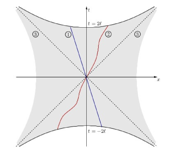
Figure 1: Conformal Representation of de Sitter Spacetime. Note that the ”observer” spacetime is interior to the Caley-Klein absolute $t^{2}-\vec{x}^{2}=4\ell^{2}$.

4 On the Geodesics of the $M^{dSL}$

In a classic book by Hawking and Ellis [15] we can read on page 126 the following statement:

de Sitter spacetime is geodesically complete; however there are points in the space which cannot be joined to each other by any geodesic.

Unfortunately many people do not realize that the points that cannot be joined by a geodesic are some points which can be joined by a spacelike curve (living in region 3 in Figure 1). So, these curves are never the path of any particle. A complete and thoughtful discussion of this issue is given in an old an excellent article by Schmidt [42].

Remark 13

Having said that, let us recall that among the Killing vector fields of $(M=\mathbb{R\times}S^{3},\boldsymbol{g})$ there are one timelike and three spacelike vector fields (which are called the translation Killing vector fields in physical literature). So, many people though since a long time ago that this permits the formulation of an energy-momentum conservation law in de Sitter spacetime $M^{dSL}$ structure . However, the fact is that what can really be done is the obtainment of conserved quantities like the $P_{\alpha}$ in Eq.(26). But we cannot obtain in $M^{dSL}$ structure an energy-momentum covector like $\boldsymbol{P}$ for a given closed physical system using an equation similar to Eq.(25). This is because de Sitter spacetime is not asymptotically flat and so there is no way to physically determine a point to fix the $\boldsymbol{\gamma}^{\alpha}$ to use in an equation similar to Eq.(25).

Now, the “translation” Killing vector fields of de Sitter spacetime are expressed in the coordinate basis $\{\partial_{\mu}=\frac{\partial}{\partial x^{\mu}}\}$ (where $\{x^{\mu}\}$ are the conformal coordinates introduced in the last section) by:

$$\mathbf{\Pi}_{\alpha}=\xi_{\alpha}^{\mu}\partial_{\mu}$$ (61)

with (putting $\ell=1$, for simplicity) are

$$\xi_{\alpha}^{\mu}=\delta_{\alpha}^{\mu}-(\frac{\eta_{\alpha\nu}x^{\nu}x^{\mu}}{2}-\frac{\sigma^{2}}{4}\delta_{\alpha}^{\mu}).$$ (62)

$$\begin{array}[c]{c}\xi_{\alpha}^{0}=\delta_{\alpha}^{0}-(\frac{\sigma^{2}}{4}\frac{\eta_{\alpha\nu}x^{\nu}x^{0}}{2}-\frac{\sigma^{2}}{4}\delta_{\alpha}^{0}),\\ \xi_{\alpha}^{1}=\delta_{\alpha}^{1}-(\frac{\sigma^{2}}{4}\frac{\eta_{\alpha\nu}x^{\nu}x^{1}}{2}-\frac{\sigma^{2}}{4}\delta_{\alpha}^{1}),\\ \xi_{\alpha}^{2}=\delta_{\alpha}^{2}-(\frac{\sigma^{2}}{4}\frac{\eta_{\alpha\nu}x^{\nu}x^{2}}{2}-\frac{\sigma^{2}}{4}\delta_{\alpha}^{2}),\\ \xi_{\alpha}^{3}=\delta_{\alpha}^{3}-(\frac{\sigma^{2}}{4}\frac{\eta_{\alpha\nu}x^{\nu}x^{3}}{2}-\frac{\sigma^{2}}{4}\delta_{\alpha}^{3}).\end{array}$$ (63)

So, we want now to investigate if there is some region of de Sitter spacetime where the “translational” Killing vector fields are linearly independent.

In order to proceed, we take an arbitrary vector field $\mathbf{V}=V^{\mu}\partial_{\mu}\in\sec T\mathcal{U}$. If the $\mathbf{\Pi}_{\alpha}$ are linearly independent in a region $\mathcal{U}^{\prime}\subset\mathcal{U}\subset\mathbb{R\times}S^{3}$ then we can write

$$\mathbf{V}=V^{\mu}\partial_{\mu}=\boldsymbol{V}^{\boldsymbol{\alpha}}\mathbf{\Pi}_{\boldsymbol{\alpha}}=\boldsymbol{V}^{\boldsymbol{\alpha}}\xi_{\boldsymbol{\alpha}}^{\mu}\partial_{\mu}.$$ (64)

So, the condition for the existence of a nontrivial solution for the $\boldsymbol{V}^{\alpha}$ is that

$$\det\left(\begin{array}[c]{cccc}\xi_{0}^{0}&\xi_{0}^{1}&\xi_{0}^{2}&\xi_{0}^{3}\\ \xi_{1}^{0}&\xi_{1}^{1}&\xi_{1}^{2}&\xi_{1}^{3}\\ \xi_{2}^{0}&\xi_{\boldsymbol{1}}^{1}&\xi_{1}^{2}&\xi_{1}^{3}\\ \xi_{3}^{0}&\xi_{3}^{1}&\xi_{3}^{2}&\xi_{3}^{3}\end{array}\right)\neq 0$$ (65)

Thus, putting

$$\chi_{\mu}:=(\frac{\sigma^{2}}{4}\frac{(x^{\mu})^{2}}{2}-\frac{\sigma^{2}}{4})$$

we need to evaluate the determinant of the matrix

$$\left(\begin{array}[c]{cccc}1-\chi_{0}&(\frac{\sigma^{2}}{4}\frac{tx}{2})&(\frac{\sigma^{2}}{4}\frac{ty}{2})&(\frac{\sigma^{2}}{4}\frac{tz}{2})\\ -(\frac{\sigma^{2}}{4}\frac{xt}{2})&1-\chi_{1}&-(\frac{\sigma^{2}}{4}\frac{xy}{2})&-(\frac{\sigma^{2}}{4}\frac{xz}{2})\\ -(\frac{\sigma^{2}}{4}\frac{yt}{2})&-(\frac{\sigma^{2}}{4}\frac{yx}{2})&1-\chi_{2}&-(\frac{yz}{\frac{m^{2}}{4}2})\\ -(\frac{\sigma^{2}}{4}\frac{zt}{2})&-(\frac{\sigma^{2}}{4}\frac{zx}{2})&-(\frac{\sigma^{2}}{4}\frac{zy}{2})&1-\chi_{3}\end{array}\right).$$ (66)

Then

$$\det[\xi_{\alpha}^{\mu}]=-\frac{1}{512}\sigma^{10}-\frac{3}{32}\sigma^{6}+\frac{1}{16}\sigma^{6}+\sigma^{2}+1-\frac{3}{128}\sigma^{8}-\frac{1}{8}\sigma^{4}$$

$$+\frac{1}{1024}\sigma^{8}(3t^{2}x^{2}y^{2}z^{2}+t^{2}y^{2}z^{2}-x^{2}y^{2}z^{2}+y^{2}z^{2})+\frac{1}{512}\sigma^{8}(t^{2}x^{2}y^{2}+t^{2}x^{2}z^{2})$$

$$+\frac{1}{128}\sigma^{6}t^{2}x^{2}(y^{2}+z^{2})+\frac{1}{256}\sigma^{6}(t^{2}y^{2}z^{2}-x^{2}y^{2}z^{2}+2y^{2}z^{2})$$

$$+\frac{1}{64}\sigma^{4}(t^{2}x^{2}y^{2}z^{2}+y^{2}z^{2}-x^{2}y^{2}z^{2})+\frac{1}{16}\sigma^{2}(t^{2}y^{2}z^{2}-^{2}x^{2}y^{2}z^{2}-2y^{2}z^{2})$$

$$+\frac{3}{8}\sigma^{4}-\frac{1}{4}y^{2}z^{2}+\frac{1}{256}\sigma^{8}.$$ (67)

In order to analyze this expression we put (without loss of generality, see the reason in [42]) $y=z=0$. In this case

$$\det[\xi_{\alpha}^{\mu}]=\frac{1}{512}\left(\sigma^{2}+4\right)^{3}\left(-\sigma^{4}+2\sigma^{2}+8\right)$$ (68)

which is null on the Caley-Klein absolute, i.e., at the points

$$t^{2}-\vec{x}^{2}=4.$$ (69)

and also on the spacelike hyperbolas given by

$$t^{2}-\vec{x}^{2}=-2\text{ and }t^{2}-\vec{x}^{2}=-4$$

So, we have proved that the translational Killing vector fields are linearly independent in all the sub region inside the Cayley-Klein absolute except in the points of the hyperbolas $t^{2}-\vec{x}^{2}=-2$ and $t^{2}-\vec{x}^{2}=-4$.

This result is very much important for the following reason. Timelike geodesics in de Sitter spacetime structure $M^{dSL}$ are (as well known) the curves $\sigma:s\rightarrow\sigma(s)$, where $s$ is propertime along $\sigma$, that extremizes the length function [28] , i.e., calling $\sigma_{\ast}=\boldsymbol{u}$ the velocity of a “particle” of mass $m$ following a time like geodesic we have that the equation of the geodesic is obtained by finding an extreme of the action, writing here in sloop notation, as

$$I[\sigma]=-m\int_{\sigma}ds=-m\int_{\sigma}(g_{\mu\nu}dx^{\mu}dx^{\nu})^{\frac{1}{2}}.$$ (70)

As well known, the determination of an extreme for $I[\sigma]$ is given by evaluating the first variation of $I[\sigma]$, i.e.,

$$\boldsymbol{\delta}^{0}I[\sigma]=m\int\pounds_{\boldsymbol{Y}}(g_{\mu\nu}dx^{\mu}dx^{\nu})^{\frac{1}{2}.}$$ (71)

and putting $\boldsymbol{\delta}^{0}I[\sigma]=0$. The result, as well known is the geodesic equation

$$\boldsymbol{D}_{\boldsymbol{u}}\boldsymbol{u}=0.$$ (72)

Now, taking into account that the Killing vector fields determines a basis inside the Cayley-Klein absolute we write

$$\boldsymbol{u}=u^{\mu}\partial_{\mu}=U^{\alpha}\mathbf{\Pi}_{\alpha}=U^{\alpha}\xi_{\alpha}^{\mu}\partial_{\mu}.$$ (73)

We now define the “hybrid” connection  coefficients $\mathbf{\Gamma}_{\cdot\mu\boldsymbol{\alpha}}^{\boldsymbol{\beta}\cdot\cdot}$  by:

$$\boldsymbol{D}_{\partial_{\mu}}\mathbf{\Pi}_{\alpha}:=\mathbf{\Gamma}_{\cdot\mu\boldsymbol{\alpha}}^{{}^{\boldsymbol{\beta}}\cdot\cdot}\Pi_{\beta},~{}~{}~{}~{}~{}\boldsymbol{D}_{\partial_{\mu}}\mathbf{\Pi}^{\alpha}:=-\mathbf{\Gamma}_{\cdot\mu\beta}^{\alpha\cdot\cdot}\mathbf{\Pi}^{\beta}$$ (74)

and write the geodesic equation as

$$\boldsymbol{D}_{\boldsymbol{u}}\boldsymbol{u}=u^{\mu}\boldsymbol{D}_{\partial\mu}(U^{\alpha}\mathbf{\Pi}_{\alpha})$$

$$=(u^{\mu}\partial_{\mu}U^{\alpha})\mathbf{\Pi}_{\alpha}+u^{\mu}U^{\alpha}\boldsymbol{D}_{\partial\mu}\mathbf{\Pi}_{\alpha}$$

$$=(u^{\mu}\partial_{\mu}U^{\boldsymbol{\beta}})\mathbf{\Pi}_{\boldsymbol{\beta}}+u^{\mu}U^{\boldsymbol{\alpha}}\mathbf{\Gamma}_{\cdot\mu\alpha}^{\beta\cdot\cdot}\mathbf{\Pi}_{\beta}$$

$$=(\frac{dU^{\beta}}{ds}+u^{\mu}U^{\alpha}\mathbf{\Gamma}_{\cdot\mu\alpha}^{\beta\cdot\cdot})\mathbf{\Pi}_{\beta}=0.$$ (75)

or

$$\frac{dU^{\beta}}{ds}+u^{\mu}U^{\alpha}\mathbf{\Gamma}_{\cdot\mu\alpha}^{\beta\cdot\cdot}=0,$$ (76)

which on multiplying by the “mass” $m$ and calling $\pi^{\beta}=mU^{\boldsymbol{\beta}}$ and $\pi_{\rho}=g_{\rho\beta}\pi^{\beta}$ can be written equivalently as

$$\frac{d\pi_{\rho}}{ds}-\mathbf{\Gamma}_{\cdot\mu\boldsymbol{\rho}}^{\beta\cdot\cdot}u^{\mu}\pi_{\beta}=0,$$ (77)

which looks like Eq.(37) in [32].

We want now to investigate the question: is Eq.(77) the same as Eq.(37) in [32]?

To know the answer to the above question recall that in [32] authors investigate the variation of $I[\sigma]$ under a variation of the curves $\sigma(s)\mapsto$ $\sigma(s,\ell)$ induced by a coordinate transformation $x^{\mu}\mapsto x^{\prime\mu}+\mathbf{\delta}_{\mathbf{\Pi}}x^{\mu}$ where they put

$$\mathbf{\delta}_{\mathbf{\Pi}}x^{\mu}=\xi_{\boldsymbol{\rho}}^{\mu}(x)\mathbf{\delta}x^{\rho}$$ (78)

with $\xi_{\boldsymbol{\rho}}^{\mu}(x)$ being the components of the Killing vector fields $\mathbf{\Pi}_{\alpha}$ (recall Eq.(62)) and where it is said that $\mathbf{\delta}x^{\rho}$ is an ordinary variation. However in [32] we cannot find what authors mean by ordinary variation, and so $\mathbf{\delta}x^{\rho}$ is not defined.

So, to continue our analysis we recall, that if the $\mathbf{\delta}x^{\rho}=\varepsilon^{\alpha}$ are constants (but arbitrary) then $\boldsymbol{\delta}_{\Pi}x^{\mu}$ corresponds to a diffeomorphism generated by a Killing vector field $\mathbf{\Pi}=\varepsilon^{\alpha}\mathbf{\Pi}_{\alpha}$. However, if the $\mathbf{\delta}x^{\rho}=\lambda^{\boldsymbol{\rho}}(x)$ are infinitesimal arbitrary functions (i.e., $\left|\lambda^{\boldsymbol{\rho}}(x)\right|<<1$), then the notation $\mathbf{\delta}_{\Pi}x^{\mu}$ is misleading since $\xi_{\boldsymbol{\rho}}^{\mu}\lambda^{\boldsymbol{\rho}}(x)$ is the $\boldsymbol{\delta}^{0}I[\sigma]$ variation generated by a quite arbitrary vector field $\boldsymbol{Y}=\lambda^{\boldsymbol{\rho}}(x)\xi_{\boldsymbol{\rho}}^{\mu}(x)\partial_{\mu}=\lambda^{\boldsymbol{\rho}}(x)\mathbf{\Pi}_{\rho}=Y^{\mu}\partial_{\mu}$. In this case we get from $\boldsymbol{\delta}^{0}I[\sigma]=0$ the geodesic equation.

4.1 Curves Obtained From Constrained Variations.

So, let us study the constrained variation when the $\mathbf{\delta}x^{\rho}=\varepsilon^{\alpha}$ are constants (but arbitrary). We denote the constrained variation by $\boldsymbol{\delta}^{c}I[\sigma]$. In this case starting from Eq.(70)

$$\boldsymbol{\delta}^{c}I[\sigma]=-m\int_{\sigma}\{u^{\gamma}(\boldsymbol{D}_{\gamma}u_{\beta})\xi_{\boldsymbol{\rho}}^{\beta}\}\mathbf{\delta}x^{\rho}ds$$ (79)

where (taking account of notations already introduced) it is

$$u^{\gamma}\boldsymbol{D}_{e_{\gamma}}(u_{\beta}e^{\beta}) =u^{\gamma}(\boldsymbol{D}_{\gamma}u_{\beta})e^{\beta},$$

$$\boldsymbol{D}_{\gamma}u_{\beta} =\partial_{\gamma}u_{\beta}-\Gamma_{\cdot\gamma\beta}^{\tau\cdot\cdot}u_{\tau},$$

$$\boldsymbol{D}_{e_{\gamma}}e_{\beta} =\Gamma_{\cdot\gamma\beta}^{\tau\cdot\cdot}e_{\tau},~{}~{}~{}\boldsymbol{D}_{e_{\gamma}}e^{\beta}=-\Gamma_{\cdot\gamma\tau}^{\beta\cdot\cdot}e^{\tau},$$ (80)

we can write

$$\boldsymbol{\delta}^{c}I[\sigma]=-m\int\{u^{\gamma}(\boldsymbol{D}_{\gamma}u_{\beta})\xi_{\boldsymbol{\rho}}^{\beta}\}\boldsymbol{\delta}x^{\rho}ds$$

$$=-m\int\{u^{\gamma}\{(\boldsymbol{D}_{\gamma}(u^{\beta}\xi_{\boldsymbol{\rho}\beta}))\}\boldsymbol{\delta}x^{\rho}ds+\frac{m}{2}\int\{u^{\gamma}u^{\beta}(\boldsymbol{D}_{\gamma}\xi_{\beta\rho}+\boldsymbol{D}_{\beta}\xi_{\rho}^{\gamma}\}\boldsymbol{\delta}x^{\rho}ds$$

$$=-m\int\{u^{\gamma}(\boldsymbol{D}_{\gamma}(\boldsymbol{u\cdot}\Pi_{\boldsymbol{\rho}}))\}\delta x^{\rho}ds=-m\int[u^{\gamma}\boldsymbol{D}_{\gamma}(\mathcal{U}_{\boldsymbol{\rho}})\}\boldsymbol{\delta}x^{\rho}ds.$$ (81)

and $\boldsymbol{\delta}^{c}I[\sigma]=0$ implies

$$u^{\gamma}\boldsymbol{D}_{\gamma}(mU_{\boldsymbol{\rho}})=0.$$ (82)

Eq.(82) with $\pi_{\boldsymbol{\rho}}=mU_{\boldsymbol{\rho}}$ can be written as

$$\frac{d}{ds}\pi_{\boldsymbol{\rho}}-u^{\gamma}\pi_{\beta}\Gamma_{\cdot\gamma\boldsymbol{\rho}}^{\beta\boldsymbol{\cdot\cdot}}=0$$ (83)

which is Eq.(37) in  [32]. Note that this equations looks like the geodesic equation written as Eq.(77) above, but it is in fact different since of course, recalling Eq.(74) it is $\mathbf{\Gamma}_{\cdot\gamma\boldsymbol{\rho}}^{\beta\boldsymbol{\cdot\cdot}}\neq\Gamma_{\cdot\gamma\boldsymbol{\rho}}^{\beta\boldsymbol{\cdot\cdot}}$. In [32] $\pi_{\boldsymbol{\rho}}=mU_{\boldsymbol{\rho}}$ is unfortunately wrongly interpreted as the components of a covector field over $\sigma$ supposed to be the energy-momentum covector of the particle, because authors of [32] supposed to have proved that this equation could be derived from Papapetrou’s method, what is not the case as we show in Section 6.

5 Generalized Energy-Momentum Conservation Laws in de Sitter Spacetime Structures

5.1 Lie Algebra of the de Sitter Group

Given a structure $(\mathring{M}\simeq\mathbb{R}^{5},\boldsymbol{\mathring{g}},)$ introduced in Section 3 define $\mathbf{J}_{AB}\in\sec T\mathring{M}$ by

$$\mathbf{J}_{AB}:=\eta_{AC}X^{C}\frac{\partial}{\partial X^{B}}-\eta_{BC}X^{C}\frac{\partial}{\partial X^{A}}.$$ (84)

These objects are generators of the Lie algebra $\mathrm{so}(1,4)$ of the de Sitter group.

Using the bases $\{\partial_{\mu}\},\{dx^{\mu}\}$ introduced above the ten Killing vector fields of de Sitter spacetime are the fields $\mathbf{J}_{\alpha 4}\in\sec TM$ and $\mathbf{J}_{\mu\nu}\in\sec TM$ and it is

$$\mathbf{J}_{\alpha 4} =\eta_{\alpha C}X^{C}\frac{\partial}{\partial X^{4}}-\eta_{4C}X^{C}\frac{\partial}{\partial X^{\alpha}}=\ell\boldsymbol{P}_{\alpha}-\frac{1}{4\ell}\boldsymbol{K}_{4\alpha}$$ (85)

$$=\ell\partial_{\alpha}-\frac{1}{4\ell}(2\eta_{\alpha\lambda}x^{\lambda}x^{\nu}-\sigma^{2}\delta_{\alpha}^{\nu})\partial_{\nu}.$$

$$\mathbf{J}_{\mu\nu} =\eta_{\mu\kappa}X^{\kappa}\frac{\partial}{\partial X^{\nu}}-\eta_{\nu\kappa}X^{\kappa}\frac{\partial}{\partial X^{\mu}}=\eta_{\mu\lambda}x^{\lambda}\boldsymbol{P}_{\nu}-\eta_{\nu\lambda}x^{\lambda}\boldsymbol{P}_{\mu}.$$ (86)

The $J_{\alpha 4}\in\sec TM$ and $J_{\mu\nu}\in\sec TM$ satisfy the Lie algebra $\mathrm{so}(1,4)$ of the de Sitter group, this time acting as a transformation group acting transitively in de Sitter spacetime. We have

$$[\mathbf{J}_{\alpha 4},\mathbf{J}_{\beta 4}] =\mathbf{J}_{\alpha\beta},$$

$$[\mathbf{J}_{\alpha\beta},\mathbf{J}_{\lambda 4}] =\eta_{\lambda\beta}\mathbf{J}_{\alpha 4}-\eta_{\lambda\alpha}\mathbf{J}_{\beta 4},$$

$$[\mathbf{J}_{\alpha\beta},\mathbf{J}_{\lambda\tau}] =\eta_{\alpha\lambda}\mathbf{J}_{\beta\tau}+\eta_{\beta\tau}\mathbf{J}_{\alpha\lambda}-\eta_{\beta\lambda}\mathbf{J}_{\alpha\tau}-\eta_{\alpha\tau}\mathbf{J}_{\beta\lambda}.$$ (87)

It is usual in physical applications to define

$$\boldsymbol{\Pi}_{\alpha}=\mathbf{J}_{\alpha 4}/\ell$$ (88)

for then we have

$$[\boldsymbol{\Pi}_{\alpha},\boldsymbol{\Pi}_{\beta}] =\frac{1}{\ell^{2}}\mathbf{J}_{\alpha\beta},$$

$$[\mathbf{J}_{\alpha\beta},\mathbf{\Pi}_{\lambda}] =\eta_{\lambda\beta}\boldsymbol{\Pi}_{\alpha}-\eta_{\lambda\alpha}\boldsymbol{\Pi}_{\beta},$$

$$[\mathbf{J}_{\alpha\beta},\mathbf{J}_{\lambda\tau}] =\eta_{\alpha\lambda}\mathbf{J}_{\beta\tau}+\eta_{\beta\tau}\mathbf{J}_{\alpha\lambda}-\eta_{\beta\lambda}\mathbf{J}_{\alpha\tau}-\eta_{\alpha\tau}\mathbf{J}_{\beta\lambda}.$$ (89)

The Killing vector fields $\mathbf{J}_{\alpha\beta}$ satisfy the Lie algebra $so(1,3)$ (of the special Lorentz group).

Remark 14

From Eq.(89) we see that when $\ell\mapsto\infty$ the Lie algebra of $so(1,4)$ goes into the Lie algebra of the Poincaré group $\mathfrak{P}$ which is the  semi-direct sum of the group of translations in $\mathbb{R}^{4}$ plus component of the special Lorentz group, i.e., $\mathfrak{P}=(\mathbb{R}^{4}\boxplus SO(1,3))$. This is eventually the justification for  physicists to call the $\boldsymbol{\Pi}_{\alpha}$ the “translation” generators of the de Sitter group.

However, it is necessary to have in mind that whereas the translation subgroup $\mathbb{R}^{4}$ of $\mathfrak{P}$ acts transitively in Minkowski spacetime manifold, the set $\{\boldsymbol{\Pi}_{\alpha}\}$ does not close in a subalgebra of the de Sitter algebra and thus it is impossible in general to find $\exp(\lambda^{\alpha}\boldsymbol{\Pi}_{\alpha})$ such that given arbitrary $x,y\in\mathbb{R\times}S^{3}$ it is $y=\exp(\lambda^{\alpha}\boldsymbol{\Pi}_{\alpha})x$. Only the whole group $SO(1,4)$ acts transitively on $\mathbb{R\times}S^{3}$.

Casimir Invariants

Now, if $\{\mathbf{E}^{A}=dX^{A}\}$ is an orthonormal basis for the structure $\mathbb{R}^{1,4}=(\mathbb{R}^{5},\boldsymbol{\mathring{g}})$ define the angular momentum operator as the Clifford algebra valued operator

$$\mathbf{J=}\frac{1}{2}\mathbf{E}^{A}\wedge\mathbf{E}^{B}\mathbf{J}_{AB}.$$ (90)

Taking into account the results of Appendix A its (Clifford) square is

$$\mathbf{J}^{2}=\mathbf{J\lrcorner J+J\wedge J=-J\cdot J+J\wedge J.}$$ (91)

It is immediate to verify that $\mathbf{J}^{2}$ is invariant under the transformations of the de Sitter group. $\mathbf{J\lrcorner J}$ is (a constant appart) the first invariant Casimir operator of the de Sitter group. The second invariant Casimir operator of the de Sitter is related to $\mathbf{J\wedge J}$. Indeed, defining

$$\mathbf{W:=}\underset{\boldsymbol{\mathring{g}}}{\star}\frac{1}{8\ell}(\mathbf{J\wedge J})=\frac{1}{8\ell}(\mathbf{J\wedge J})\lrcorner\tau_{\boldsymbol{\mathring{g}}}.$$ (92)

one can easily show (details in [39]) that

$$\mathbf{W\cdot W} =\mathbf{WW}=\mathbf{W}^{2}=-\frac{1}{64\ell^{2}}(\mathbf{J\wedge J})\lrcorner(\mathbf{J\wedge J})=-\frac{1}{64\ell^{2}}(\mathbf{J\wedge J})\cdot(\mathbf{J\wedge J})$$

$$=-\frac{1}{64\ell^{2}}(\mathbf{J\wedge J})(\mathbf{J\wedge J}).$$ (93)

is indeed an invariant operator.

As well known, the representations of the de Sitter group are classified by their Casimir invariants $I_{1}$ and $I_{2}$ which here following [14] we take as

$$I_{1} =-\mathbf{J\lrcorner J=}\frac{1}{2\ell^{2}}\mathbf{J}_{AB}\mathbf{J}^{AB}=\eta^{\alpha\beta}\boldsymbol{\Pi}_{\alpha}\boldsymbol{\Pi}_{\beta}+\frac{1}{2\ell^{2}}\text{ }\eta^{\alpha\lambda}\eta^{\beta\tau}\mathbf{J}_{\alpha\beta}\mathbf{J}_{\lambda\tau}=M^{2},$$

$$I_{2} =\mathbf{W}^{2}=\boldsymbol{W}^{A}\boldsymbol{W}_{A}=\eta^{\alpha\beta}\boldsymbol{V}_{\alpha}\boldsymbol{V}_{\beta}+\frac{1}{\ell^{2}}(\boldsymbol{W}_{4})^{2},$$ (94)

where $M\in\mathbb{R}$ and the fields $\boldsymbol{W}_{A}$ and $\boldsymbol{V}_{\alpha}$ are defined by:

$$\boldsymbol{W}_{A} :=\frac{1}{8\ell}\varepsilon_{ABCDE}\mathbf{J}^{AB}\mathbf{J}^{DE}$$

$$\boldsymbol{V}_{\alpha} :=-\frac{1}{2}\varepsilon_{4\alpha\lambda\mu\nu}\eta^{\lambda\rho}\boldsymbol{\Pi}_{\rho}\mathbf{J}^{\mu\nu},$$ (95)

from where it follows that

$$\boldsymbol{W}_{4}=\frac{1}{8}\varepsilon_{4\mu\nu\rho\tau}\mathbf{J}^{\mu\nu}\mathbf{J}^{\mu\nu}.$$ (96)

In the limit when $\ell\mapsto\infty$ we get the Casimir operators of the special Lorentz group

$$I_{1} \mapsto\boldsymbol{P}_{\alpha}\boldsymbol{P}^{\alpha}=m^{2}\mathbf{,}$$

$$I_{2} \mapsto\eta^{\alpha\beta}\boldsymbol{V}_{\alpha}\boldsymbol{V}_{\beta}=m^{2}s(s+1)$$ (97)

where $m\in\mathbb{R}$ and $s=0,1/2,1,3/2,...$

We see that $\boldsymbol{\Pi}_{\alpha}$ looks like the components of an energy-momentum vector $\boldsymbol{P}=\left.P_{\alpha}\vartheta^{\alpha}\right|_{o}$ of a closed physical system (see Eq.(25)) in the Minkowski spacetime of Special Relativity, for which $\boldsymbol{P}^{2}=m^{2}$, with $m$ the mass of the system. However, take into account that whereas the $P_{\alpha}$ are simple real numbers, the $\boldsymbol{\Pi}_{\alpha}$ are vector fields.

Moreover, take into account that $\eta^{\alpha\beta}\boldsymbol{\Pi}_{\alpha}\boldsymbol{\Pi}_{\beta}$ is not an invariant, i.e., it does not commute with the generators of the Lie algebra of the de Sitter group.

5.2 Generalized Energy-Momentum Covector for a Closed System in the Teleparallel de Sitter Spacetime Structure

In this section we suppose that $(M=\mathbb{R\times}S^{3},\boldsymbol{g},\tau_{\boldsymbol{g}},\uparrow)$ is the physical arena where Physics take place.

We know that $(M=\mathbb{R\times}S^{3},\boldsymbol{g}$) has ten Killing vector fields and four of them (one timelike and three spacelike, $\boldsymbol{\Pi}_{\alpha}$, $\alpha=0,1,2,3$ ) generated “translations”. Thus if we suppose that $(M=\mathbb{R\times}S^{3},\boldsymbol{g},\tau_{\boldsymbol{g}},\uparrow)$ is populated by interacting matter fields $\{\phi_{1,}...,\phi_{n}\}$ with dynamics described by a Lagrangian formalism we can construct as described in the Appendix C.1 the conserved currents

$$\mathcal{J}_{\mathbf{\Pi}_{\alpha}}=\mathcal{J}_{\alpha}^{\beta}\boldsymbol{\gamma}_{\beta}=\mathcal{J}_{\alpha}^{\mu}\boldsymbol{\vartheta}_{\mu}$$ (98)

were taking into account that $\boldsymbol{\delta}_{\mathbf{\Pi}_{\alpha}}^{0}=-\pounds_{\mathbf{\Pi}_{\alpha}}$ and denoting by $\boldsymbol{\delta}_{\mathbf{\Pi}_{\alpha}}$ each particular local variation generated by $\mathbf{\Pi}_{\alpha}$ (recall Eq.(61)) we have

$$\boldsymbol{\delta}_{\mathbf{\Pi}_{\alpha}}\phi_{A}=\boldsymbol{\delta}_{\mathbf{\Pi}_{\alpha}}^{0}\phi_{A}+\mathbf{\delta}x^{\nu}\partial_{\nu}\phi_{A}$$ (99)

and thus we write

$$\mathcal{J}_{\alpha}^{\mu} =\pi_{A}^{\mu}\boldsymbol{\delta}_{\mathbf{\Pi}_{\alpha}}\phi_{A}+\Upsilon_{\nu}^{\mu}\boldsymbol{\delta}_{\mathbf{\Pi}_{\alpha}}^{0}x^{\mu}$$

$$=\Lambda_{\nu}^{\mu}\boldsymbol{\xi}_{\alpha}^{\nu}+\Upsilon_{\nu}^{\mu}\boldsymbol{\xi}_{\alpha}^{\nu}$$ (100)

where

$$\Lambda_{\nu}^{\mu}\boldsymbol{\xi}_{\alpha}^{\nu}:=\pi_{A}^{\mu}\boldsymbol{\delta}_{\mathbf{\Pi}_{\alpha}}\phi_{A}.$$ (101)

In Eq.(98) $\{\boldsymbol{\gamma}^{\beta}\}$ is the dual basis of the orthonormal basis $\{\boldsymbol{e}_{\alpha}\}$ defined by

$$\boldsymbol{e}_{\alpha}:=\frac{\boldsymbol{\Pi}_{\alpha}}{\boldsymbol{g}(\boldsymbol{\Pi}_{\alpha},\boldsymbol{\Pi}_{\alpha})}.$$ (102)

From the conserved currents $\mathcal{J}_{\mathbf{\Pi}_{\alpha}}$ we can obtain four conserved quantities (the $P_{\alpha}$ in Eq.(26)).

Remark 15

It is crucial to observe that the above results have been deduced without introduction of any connection in the structure $(M=\mathbb{R\times}S^{3},\boldsymbol{g,}\tau_{\boldsymbol{g}},\uparrow)$. However that structure is not enough for using the $P_{\alpha}$ to build a (generalized) covector analogous to the energy-momentum covector $\boldsymbol{P}$ (see Eq.(25)) of special relativistic theories.

If we add $\boldsymbol{D}$, the Levi-Civita connection of $\boldsymbol{g}$ to $(M=\mathbb{R\times}S^{3},\boldsymbol{g,}\tau_{\boldsymbol{g}},\uparrow)$ we get the Lorentzian de Sitter spacetime structure $M^{dSP}$ and defining a generalized energy-momentum tensor

$$\mathbf{\Theta}=\mathcal{J}_{\mathbf{\Pi}_{\alpha}}\otimes e^{\alpha}\in\sec T_{1}^{1}M$$ (103)

we know that $\underset{\boldsymbol{g}}{\delta}\mathcal{J}_{\mathbf{\Pi}_{\alpha}}=0$ implies $\boldsymbol{D}\cdot\mathbf{\Theta}=0$, a covariant “conservation” law.

However, the introduction of $M^{dSP}$ in our game is of no help to construct a covector like $\boldsymbol{P}$ since in $M^{dSP}$ vectors at different spacetime points cannot be directly compared..

So, the question arises: is it possible to define a structure where $\forall x,y\in\mathbb{R\times}S^{3}$ we can define objects $P_{\alpha}^{\mathrm{dS}}$ such that

$$\boldsymbol{P}_{\mathrm{dS}}=P_{\alpha}^{\mathrm{dS}}\left.\boldsymbol{\gamma}^{\alpha}\right|_{x}=P_{\alpha}^{\mathrm{dS}}\left.\boldsymbol{\gamma}^{\alpha}\right|_{y}$$ (104)

defines a legitimate covector for a closed physical system living in a de Sitter structure $(M=\mathbb{R\times}S^{3},\boldsymbol{g,}\tau_{\boldsymbol{g}},\uparrow)$ and for which $\boldsymbol{P}_{\mathrm{dS}}$ can be said to be a kind of generalization of the momentum of the closed system in Minkowski spacetime?

We show now the answer is positive. We recall that $\boldsymbol{D}$ has been introduced in our developments only as a useful mathematical device and is quite irrelevant in the construction of legitimate conservation laws since the conserved currents $\mathcal{J}_{\mathbf{\Pi}_{\alpha}}$ have been obtained without the use of any connection. So, we now introduce for our goal a teleparallel de Sitter spacetime, i.e., the structure $M^{dSTP}=(M=\mathbb{R\times}S^{3},\boldsymbol{\nabla},\tau_{\boldsymbol{g}},\uparrow)$ where $\boldsymbol{\nabla}$ is a metric compatible teleparallel connection defined by

$$\boldsymbol{\nabla}_{\boldsymbol{e}_{\alpha}}\boldsymbol{e}_{\beta}=\omega_{\cdot\alpha\beta}^{\kappa\cdot\cdot}\boldsymbol{e}_{\kappa}=0.$$ (105)

Under this condition we know that we can identify all tangent and all cotangent spaces. So, we have for $\forall x,y\in\mathbb{R\times}S^{3},$

$$\left.\boldsymbol{e}_{\alpha}\right|_{x}\simeq\left.\boldsymbol{e}_{\alpha}\right|_{y}\text{~{}~{}and~{}~{}}\left.\boldsymbol{\gamma}^{\alpha}\right|_{x}\simeq\left.\boldsymbol{\gamma}^{\alpha}\right|_{y}=\boldsymbol{E}^{\alpha},$$

where $\{\boldsymbol{E}^{\alpha}\}$ is a basis of a vector space $\mathcal{V\simeq}\mathbb{R}^{4}$.

Thus, in the structure $M^{dSTP}$ Eq.(104) defines indeed a legitimate covector in $\mathcal{V\simeq}\mathbb{R}^{4}$ and thus permits a legitimate generalization of the concepts of energy-momentum covector obtained for physical theories in Minkowski spacetime. The term generalization is a good one here because in the limit where $\ell\rightarrow\infty$, $\boldsymbol{\Pi}_{\alpha}\mapsto\partial/\partial x^{\alpha},$ $\Lambda_{\alpha}^{\kappa}=0$ and thus $\Theta_{\alpha}^{\kappa}=\Upsilon_{\alpha}^{\kappa}$.

5.3 The Conserved Currents $\boldsymbol{J}_{\mathbf{\Pi}_{\alpha}}=\boldsymbol{g}(\boldsymbol{\Pi}_{\alpha},\boldsymbol{~{}})$

To proceed we show that the translational Killing vector fields of the de Sitter structure $(M,\boldsymbol{g})$ determines trivially conserved currents

$$\boldsymbol{J}_{\mathbf{\Pi}_{\alpha}}=\boldsymbol{g}(\boldsymbol{\Pi}_{\alpha},\boldsymbol{~{}})$$

Indeed  using the $M^{dSTP}$ structure as a convenient device we recall the result proved in [35] that for each vector Killing $\mathbf{K}$ the one form field $K=\boldsymbol{g}(\mathbf{K},\boldsymbol{~{}})$ is such that $\underset{\boldsymbol{g}}{\delta}K=0$. So, it is

$$\underset{\boldsymbol{g}}{\delta}\boldsymbol{J}_{\mathbf{\Pi}_{\alpha}}=0.$$ (106)

and of course, also

$$\underset{\boldsymbol{g}}{\delta}\boldsymbol{J}_{\mathbf{\Pi}}=0$$ (107)

where

$$\boldsymbol{J}_{\mathbf{\Pi}}:=\boldsymbol{g}(\boldsymbol{\Pi},\boldsymbol{~{}}),~{}~{}~{}~{}\boldsymbol{\Pi:=\varepsilon}^{\alpha}\boldsymbol{\Pi}_{\alpha}$$ (108)

with the $\boldsymbol{\varepsilon}^{\alpha}$ real constants such that $\left|\boldsymbol{\varepsilon}^{\alpha}\right|<<1$. Recalling from Eq.(86) that in projective conformal coordinate bases ($\{e_{\mu}=\partial_{\mu}\}$ and $\{\boldsymbol{\vartheta}^{\mu}=dx^{\mu}\}$) the components of $\boldsymbol{\Pi}_{\alpha}$ are

$$\xi_{\alpha}^{\mu}=\delta_{\alpha}^{\mu}-\frac{1}{4\ell^{2}}(2\eta_{\alpha\rho}x^{\rho}x^{\mu}-\sigma^{2}\delta_{\alpha}^{\mu})$$ (109)

we get the conserved current $\boldsymbol{J}_{\mathbf{\Pi}}$ is

$$\boldsymbol{J}_{\mathbf{\Pi}}=\boldsymbol{\varepsilon}^{\alpha}\boldsymbol{J}_{\mathbf{\Pi}_{\alpha}}=\boldsymbol{\varepsilon}^{\alpha}\xi_{\alpha}^{\mu}\boldsymbol{\vartheta}_{\mu}.$$ (110)

Remark 16

Take notice that of course, this current is not the conserved current that we found in the previous section.

Remark 17

Take notice also that in [32] authors trying to generalize the results that follows from the canonical formalism for the case of field theories in Minkowski spacetime suppose that they can eliminate the term $\pi_{A}^{\mu}\boldsymbol{\delta}\phi_{A}$ from Eq.(100) by decree postulating a “new kind of “local variation”, call it $\boldsymbol{\delta}^{\prime}$ for which $\boldsymbol{\delta}^{\prime}\phi_{A}=0$. The fact is that such a “new kind of local variation” never appears in the canonical Lagrangian formalism, only $\boldsymbol{\delta}\phi_{A}$ appears and in general it is not zero.

Now, the generalized canonical de Sitter energy-momentum tensor is

$$\mathbf{\Theta}=\mathcal{J}_{\mathbf{\Pi}_{\alpha}}\otimes e^{\alpha}=\Theta_{\alpha}^{\kappa}\boldsymbol{\vartheta}_{\kappa}\otimes e^{\alpha}\in\sec\bigwedge\nolimits^{1}T^{\ast}M\otimes TM$$ (111)

and making analogy with the case of Minkowski spacetime where the $\Upsilon_{\alpha}^{\kappa}$ have been defined as the components of the canonical energy-momentum tensor $\boldsymbol{\Upsilon}$, we write $\Theta_{\alpha}^{\kappa},$ as

$$\Theta_{\alpha}^{\kappa}=\Upsilon_{\alpha}^{\kappa}-\frac{1}{4\ell^{2}}K_{\alpha}^{\kappa}+\Lambda_{\alpha}^{\kappa},$$ (112)

Thus each one of the genuine conservation laws $d\underset{\boldsymbol{g}}{\star}\mathcal{J}_{\mathbf{\Pi}_{\alpha}}=0$, $\alpha=0,1,2,3$ read in coordinate basis components

$$(\partial_{\mu}\Upsilon_{\alpha}^{\kappa}-\Gamma_{\cdot\lambda\nu}^{\lambda\cdot\cdot}\Upsilon_{\alpha}^{\kappa})-\frac{1}{4\ell^{2}}(\partial_{\mu}K_{\alpha}^{\mu}-\Gamma_{\cdot\lambda\nu}^{\lambda\cdot\cdot}K_{\alpha}^{\kappa})-(\partial_{\mu}\Lambda_{\alpha}^{\kappa}-\Gamma_{\cdot\lambda\nu}^{\lambda\cdot\cdot}\Lambda_{\alpha}^{\kappa})$$

$$=\frac{1}{\sqrt{-\det\boldsymbol{g}}}\partial_{\mu}(\sqrt{-\det\boldsymbol{g}}\Upsilon_{\alpha}^{\mu})-\frac{1}{4\ell^{2}}\frac{1}{\sqrt{-\det\boldsymbol{g}}}\partial_{\mu}(\sqrt{-\det\boldsymbol{g}}K_{\alpha}^{\mu})$$ (113)

$$+\frac{1}{\sqrt{-\det\boldsymbol{g}}}\partial_{\mu}(\sqrt{-\det\boldsymbol{g}}\Lambda_{\alpha}^{\mu})=0$$

or

$$\partial_{\mu}\left[\sqrt{-\det\boldsymbol{g}}\left(\Upsilon_{\alpha}^{\mu}-\frac{1}{4\ell^{2}}K_{\alpha}^{\mu}+\Lambda_{\alpha}^{\mu}\right)\right]=0\Leftrightarrow\boldsymbol{D}_{\mu}\Theta_{\alpha}^{\mu}=0.$$ (114)

Remark 18

Now, recalling the relation of the connection coefficients of the bases $\{\boldsymbol{e}_{\alpha}\}$ of the Levi-Civita connection $\boldsymbol{D}$ of $\boldsymbol{g}$ (denoted $\mathbf{\Gamma}_{\cdot\alpha\beta}^{\kappa\cdot\cdot}$) and the coefficients of the basis $\{\boldsymbol{e}_{\alpha}\}$ of the teleparallel connection $\nabla$ of $\boldsymbol{g}$ (denoted $\mathbf{\bar{\Gamma}}_{\cdot\alpha\beta}^{\kappa\cdot\cdot}$) are [34]

$$\mathbf{\bar{\Gamma}}_{\cdot\alpha\beta}^{\kappa\cdot\cdot}=\mathbf{\Gamma}_{\cdot\alpha\beta}^{\kappa\cdot\cdot}+\mathrm{\triangle}_{\cdot\alpha\beta}^{\kappa\cdot\cdot}$$ (115)

where

$$\mathrm{\triangle}_{\cdot\alpha\beta}^{\kappa\cdot\cdot}:=-\frac{1}{2}\left(\mathrm{T}_{\alpha\cdot\beta}^{\cdot\kappa\cdot}+\mathrm{T}_{\beta\cdot\alpha}^{\cdot\kappa\cdot}-\mathrm{T}_{\cdot\alpha\beta}^{\kappa\cdot\cdot}\right)$$ (116)

are the components of the contorsion tensor and $\mathrm{T}_{\cdot\alpha\beta}^{\kappa\cdot\cdot}$ are the components of the torsion tensor of the connection $\nabla$, we can write $\boldsymbol{D}\bullet\boldsymbol{\Theta}=0$ (taking into account that $\mathbf{\bar{\Gamma}}_{\cdot\alpha\beta}^{\kappa\cdot\cdot}=0$) in components relative to orthonormal basis as

$$\boldsymbol{D}_{\alpha}\Theta_{\beta}^{\alpha}:=(\boldsymbol{D}_{\boldsymbol{e}_{\alpha}}\boldsymbol{\Theta})_{\beta}^{\alpha}=\boldsymbol{e}_{\alpha}(\Theta_{\beta}^{\alpha})+\mathrm{\triangle}_{\alpha\iota}^{\alpha}\Theta_{\beta}^{\iota}-\mathrm{\triangle}_{\alpha\beta}^{\iota}\Theta_{\iota}^{\alpha}=0.$$

On the other hand since $\nabla_{\alpha}\Theta_{\beta}^{\alpha}:=(\nabla_{\boldsymbol{e}_{\alpha}}\Theta)_{\beta}^{\alpha}=\boldsymbol{e}_{\alpha}(\Theta_{\beta}^{\alpha})$ we have

$$\nabla_{\alpha}\Theta_{\beta}^{\alpha}=-\mathrm{\triangle}_{\alpha\iota}^{\alpha}\Theta_{\beta}^{\iota}+\mathrm{\triangle}_{\alpha\beta}^{\iota}\Theta_{\iota}^{\alpha},$$ (117)

which means that although $(\nabla\bullet\boldsymbol{\Theta})_{\beta}^{\alpha}:=\nabla_{\alpha}\Theta_{\beta}^{\alpha}\neq 0$ we can generate the conserved currents $\boldsymbol{J}_{\mathbf{\Pi}_{\alpha}}$ in the teleparallel de Sitter spacetime structure if Eq.(117) is satisfied.

Remark 19

To end this section and for completeness of the article it is necessary to mention that in a remarkable paper ([9]) the gravitational energy-momentum tensor  in teleparallel gravity is discused in details. Also related papers are ([10, 24]). A complete list of references can be found in ([1])

6 Equation of Motion for a Single-Pole Mass in a GRT Lorentzian Spacetime

In a classical paper Papapetrou derived the equations of motion of single pole and spinning particles in GRT. Here we recall his derivation for the case of a single pole-mass. We start recalling that in GRT the matter fields is described by a energy-mometum tensor that satisfies the covariant conservation law $\boldsymbol{D}\bullet\boldsymbol{T}=0$. If we introduce the relative tensor

$$\mathfrak{T=}\boldsymbol{T\otimes\tau}_{\boldsymbol{g}}\in\sec T_{1}^{1}M\otimes{\textstyle\bigwedge\nolimits^{4}}T^{\ast}M$$ (118)

we have recalling Appendix E and that $\boldsymbol{D}\bullet\boldsymbol{T}=0$ that

$$\boldsymbol{D}_{\nu}\mathfrak{T}^{\mu\nu}+\Gamma_{\cdot\nu\alpha}^{\mu\cdot\cdot}\mathfrak{T}^{\alpha\nu}=0.$$ (119)

From Eq.(119) we have

$$\partial_{\nu}(x^{\alpha}\mathfrak{T}^{\mu\nu})=\mathfrak{T}^{\mu\alpha}-x^{\alpha}\Gamma_{\cdot\nu\alpha}^{\mu\cdot\cdot}\mathfrak{T}^{\alpha\nu}.$$ (120)

To continue we suppose that a single-pole mass (considered as a probe particle) is modelled by the restriction of the energy-mometum tensor $\boldsymbol{T}$ inside a “narrow” tube in the Lorentzian spacetime representing a given gravitational field. Let us call $\boldsymbol{T}_{0}$ that restriction and notice that $\boldsymbol{D}\bullet\boldsymbol{T}_{0}=0$. Inside the tube a timelike line $\gamma$ is chosen to represent the particle motion. We restrict our analysis to hyperbolic Lorentzian spacetimes for which a foliation $\mathbb{R\times}\mathcal{S}$ ($\mathcal{S}$ a $3$-dimensional manifold) exists. We choose a parametrization for $\gamma$ such that the its coordinates are $\boldsymbol{x}^{\mu}(\gamma(t))=\mathrm{X}^{\mu}(t)$ where $t=x^{0}$. The probe particle is characterized by taking the coordinates of any point in the world tube to satisfy

$$\mathrm{\delta}x^{\mu}=x^{\mu}-\mathrm{X}^{\mu}<<1.$$ (121)

According to Papapetrou a single-pole particle is one for which the integral

$$\int\mathfrak{T}_{o}^{\mu\nu}dv\neq 0,$$ (122)

and all other integrals

$$\int\mathrm{\delta}x^{\alpha}\mathfrak{T}_{o}^{\mu\nu}dv,~{}~{}~{}\int\mathrm{\delta}x^{\alpha}\mathrm{\delta}x^{\beta}\mathfrak{T}_{o}^{\mu\nu}dv,...$$ (123)

are null. We now evaluate

$$\frac{d}{dt}\int\mathfrak{T}_{o}^{\mu 0}=-\int\Gamma_{\cdot\nu\alpha}^{\mu\cdot\cdot}\mathfrak{T}_{o}^{\alpha\nu}dv$$ (124)

and

$$\frac{d}{dt}\int x^{\alpha}\mathfrak{T}_{o}^{\mu 0}=\int\mathfrak{T}_{o}^{\mu\alpha}dv-\int x^{\alpha}\Gamma_{\cdot\nu\alpha}^{\mu\cdot\cdot}\mathfrak{T}_{o}^{\alpha\nu}dv.$$ (125)

Inside the world tube modelling the particle we can expand the connection coefficients as

$$\Gamma_{\cdot\nu\alpha}^{\mu\cdot\cdot}=\text{~{}}_{o}\Gamma_{\cdot\nu\alpha}^{\mu\cdot\cdot}+~{}_{o}\Gamma_{\cdot\nu\alpha,\kappa}^{\mu\cdot\cdot}\mathrm{\delta}x^{\kappa}$$ (126)

with  ${}_{o}\Gamma_{\cdot\nu\alpha}^{\mu\cdot\cdot}$ the components of the connection in the worldline $\gamma$. Then according to the definition of a single-pole particle we get from Eq.(124) and Eq.(125) along $\gamma$:

$$\frac{d}{dt}\int\mathfrak{T}_{o}^{\mu 0}+\text{~{}}_{o}\Gamma_{\cdot\nu\alpha}^{\mu\cdot\cdot}\int\mathfrak{T}_{o}^{\alpha\nu}=0,$$ (127)

$$\int\mathfrak{T}_{o}^{\mu\alpha}=\frac{d\mathrm{X}^{\mu}}{dt}\int\mathfrak{T}_{o}^{\nu 0}dv.$$ (128)

Now, put

$$\gamma_{\ast}=\boldsymbol{u}:=\frac{d\mathrm{X}^{\mu}}{ds}e_{\mu}$$ (129)

where $ds$ is proper time along $\gamma$ and define

$$M^{\mu\alpha}=u^{0}\int\mathfrak{T}_{o}^{\mu\alpha}dv.$$ (130)

Eq.(127) and Eq.(128) become

$$\frac{d}{ds}\left(\frac{M^{\mu 0}}{u^{0}}\right)+\text{~{}}_{o}\Gamma_{\cdot\nu\alpha}^{\mu\cdot\cdot}M^{\alpha\nu}=0$$ (131)

and

$$M^{\mu\alpha}=u^{\mu}\frac{M^{\alpha 0}}{u^{0}}.$$ (132)

So, $M^{\mu 0}=u^{\mu}\frac{M^{00}}{u^{0}}$ from where it follows that putting

$$m:=\frac{M^{00}}{(u^{0})^{2}}$$ (133)

it is

$$M^{\mu\alpha}=u^{\mu}\frac{M^{\alpha 0}}{u^{0}}=mu^{\mu}u^{\alpha}$$ (134)

and we get

$$\frac{d}{ds}(mu^{\mu})+~{}_{o}\Gamma_{\cdot\nu\alpha}^{\mu\cdot\cdot}mu^{\nu}u^{\alpha}=0.$$ (135)

Now, the acceleration of the probe particle is $\boldsymbol{a}:=\boldsymbol{D}_{\boldsymbol{u}}\boldsymbol{u}$ and thus $\boldsymbol{g}(\boldsymbol{a,u})=0$, i.e.,

$$u_{\mu}\frac{d}{ds}u^{\mu}+~{}_{o}\Gamma_{\cdot\nu\alpha}^{\mu\cdot\cdot}mu^{\nu}u^{\alpha}u_{\mu}=0.$$ (136)

Multiplying Eq.(135) by $u_{\mu}$ and using Eq.(136) gives

$$\frac{d}{ds}m=0$$ (137)

and then Eq.(135) says that $\gamma$ is a geodesic of the Lorentzian spacetime structure, i.e.,

$$\boldsymbol{D}_{\gamma_{\ast}}\gamma_{\ast}=0$$ (138)

or

$$\frac{du^{\mu}}{ds}+~{}_{o}\Gamma_{\cdot\nu\alpha}^{\mu\cdot\cdot}mu^{\nu}u^{\alpha}=0.$$

7 Equation of Motion for a Single-Pole Mass in a de Sitter Lorentzian Spacetime

In this section we suppose that the arena where physical events take place is the de Sitter spacetime structure $M^{dS\ell}$ where fields live and interact, without never changing the metric $\boldsymbol{g}$, which we emphasize do not represent any gravitational field here, i.e., we do not suppose here that $M^{dS\ell}$ is a model of a gravitational field in GRT. As we learned in Section 4 since de Sitter spacetime has one timelike and three spacelike Killing vector fields $\mathbf{\Pi}_{\alpha}$ we can construct the conserved currents $\mathcal{J}_{\mathbf{\Pi}_{\alpha}}=\Theta_{\alpha}^{\mu}\boldsymbol{\vartheta}_{\mu}$ (see Eq.(98)) from where we get $\boldsymbol{D}\bullet\mathbf{\Theta}=0$ with $\mathbf{\Theta}=\mathcal{J}_{\mathbf{\Pi}_{\alpha}}\otimes e^{\alpha}=\Theta_{\alpha}^{\kappa}\boldsymbol{\vartheta}_{\kappa}\otimes e^{\alpha}$.

Now, if we suppose that a probe free single-pole particle (i.e., one for which its interaction with the remaining fields can be despised) is described by a covariant conserved tensor $\mathbf{\Theta}$ in a narrow tube like the one introduced in the previous section, we can derive (using analog notations for $\gamma$, etc…) an equation like Eq.(127), i.e.,

$$\frac{d}{dt}\int\Theta_{o}^{\mu 0}\sqrt{-\det\boldsymbol{g}_{o}}dv+\text{~{}}_{o}\Gamma_{\cdot\nu\alpha}^{\mu\cdot\cdot}\int\Theta_{o}^{\alpha\nu}\sqrt{-\det\boldsymbol{g}_{o}}dv=0.$$ (139)

Now, we obtain an equation analogous to Eq.(131) with $M^{\alpha\nu}$ substituted by $N^{\alpha\nu}$ i.e.,

$$\frac{d}{ds}\left(\frac{N^{\mu 0}}{u^{0}}\right)+\text{~{}}_{o}\Gamma_{\cdot\nu\alpha}^{\mu\cdot\cdot}N^{\alpha\nu}=0$$ (140)

with

$$N^{\alpha\nu}:=u^{0}\int\Theta_{o}^{\mu\alpha}\sqrt{-\det\boldsymbol{g}_{o}}dv.$$ (141)

Putting this time

$$m:=\frac{N^{00}}{(u^{0})^{2}}$$ (142)

we get $N^{\mu\alpha}=u^{\mu}\frac{N^{\alpha 0}}{u^{0}}=mu^{\mu}u^{\alpha}$ and

$$\frac{d}{ds}(mu^{\mu})+~{}_{o}\Gamma_{\cdot\nu\alpha}^{\mu\cdot\cdot}mu^{\nu}u^{\alpha}=0,$$ (143)

from where we get exactly as in the previous section that $m=const$ and $\boldsymbol{D}_{\gamma_{\ast}}\gamma_{\ast}=0$.

Conclusion 20

Papapetrou method applied to the $M^{dS\ell}$ structure gives for the motion of a free single pole particle the geodesic equation $\boldsymbol{D}_{\gamma_{\ast}}\gamma_{\ast}=0$. Moreover, Eq.(143) is of course, different from Eq.(83) contrary to conclusions of authors of  [32]. It is also to be noted here that in [32] authors inferred correctly that Papapetrou method leads to an equation that looks like to Eq.(139) for a single-pole particle moving in the $M^{dS\ell}$ structure. The equation that looks like Eq.(139) in [32] is the Eq.(37) there, but where in the place of $\Theta_{o}^{\alpha\nu}$ they used $\Upsilon_{o}^{\alpha\nu}-\frac{1}{4\ell^{2}}\Upsilon_{o}^{\alpha\nu}$, because they believe to be possible to use a local variation of the fields that results in $\Lambda_{\nu}^{\mu}=0$.

Appendix A Clifford Bundle Formalism

Let $(M,\boldsymbol{g},D,\tau_{\boldsymbol{g}},\uparrow)$ be an arbitrary Lorentzian or Riemann-Cartan spacetime structure. The quadruple $(M,\boldsymbol{g},\tau_{\boldsymbol{g}},\uparrow)$ denotes a four-dimensional time-oriented and space-oriented Lorentzian manifold [34, 43]. This means that $\boldsymbol{g}\in\sec T_{2}^{0}M$ is a Lorentzian metric of signature $(1,3)$, $\tau_{\boldsymbol{g}}\in\sec\bigwedge{}^{4}T^{\ast}M$ and $\uparrow$ is a time-orientation (see details, e.g., in [43]). Here, $T^{\ast}M$ [$TM$] is the cotangent [tangent] bundle. $T^{\ast}M=\cup_{x\in M}T_{x}^{\ast}M$, $TM=\cup_{x\in M}T_{x}M$, and $T_{x}M\simeq T_{x}^{\ast}M\simeq\mathbb{R}^{1,3}$, where $\mathbb{R}^{1,3}$ is the Minkowski vector space. $D$ is a metric compatible connection, i.e., $D\boldsymbol{g}=0$. When $D=\boldsymbol{D}$ is the Levi-Civita connection of $\boldsymbol{g}$ , $\mathbf{R}^{\boldsymbol{D}}\neq 0$, and $\Theta^{\boldsymbol{D}}=0$, $\mathbf{R}^{\boldsymbol{D}}$ and $\Theta^{\boldsymbol{D}}$ being respectively the curvature and torsion tensors of the connection. $D=\boldsymbol{\nabla}$ is is a Riemann-Cartan connection , $\mathbf{R}^{\boldsymbol{\nabla}}\neq 0$, and $\Theta^{\boldsymbol{\nabla}}\neq 0$ Let $\mathtt{g}\in\sec T_{0}^{2}M$ be the metric of the cotangent bundle. The Clifford bundle of differential forms $\mathcal{C}\ell(M,\mathtt{g})$ is the bundle of algebras, i.e., $\mathcal{C}\ell(M,\mathtt{g})=\cup_{x\in M}\mathcal{C}\ell(T_{x}^{\ast}M,\mathtt{g})$, where $\forall x\in M$, $\mathcal{C}\ell(T_{x}^{\ast}M,\mathtt{g})=\mathbb{R}_{1,3}$, the so called spacetime algebra [34]. Recall also that $\mathcal{C}\ell(M,\mathtt{g})$ is a vector bundle associated to the orthonormal frame bundle, i.e., we have $\mathcal{C}\ell(M,\mathtt{g})$ $=P_{\mathrm{SO}_{(1,3)}^{e}}(M)\times_{\mathrm{Ad}^{\prime}}\mathbb{R}_{1,3}$ [21, 25]. Also, when $(M,\boldsymbol{g)}$ is a spin manifold we can show that $\mathcal{C}\ell(M,\mathtt{g})$ $=P_{\mathrm{Spin}_{(1,3)}^{e}}(M)\times_{\mathrm{Ad}}\mathbb{R}_{1,3}$ For any $x\in M$, $\mathcal{C}\ell(T_{x}^{\ast}M,\left.\mathtt{g}\right|_{x})$ as a linear space over the real field $\mathbb{R}$ is isomorphic to the Cartan algebra $\bigwedge T_{x}^{\ast}M$ of the cotangent space. We have that $\bigwedge{}_{x}^{\ast}M=\oplus_{k=0}^{4}\bigwedge^{k}T_{x}^{\ast}M$, where $\bigwedge^{k}T_{x}^{\ast}M$ is the $\binom{4}{k}$-dimensional space of $k$-forms. Then, sections of $\mathcal{C}\ell(M,\mathtt{g})$ can be represented as a sum of non homogeneous differential forms, that will be called Clifford (multiform) fields. In the Clifford bundle formalism, of course, arbitrary basis can be used, but in this short review of the main ideas of the Clifford calculus we use mainly orthonormal basis. Let then $\{\boldsymbol{e}_{\mathbf{\alpha}}\}$ be an orthonormal basis for $TU\subset TM$, i.e., $\mathtt{g}(\boldsymbol{e}_{\mathbf{\alpha}},\boldsymbol{e}_{\mathbf{\beta}})=\eta_{\mathbf{\alpha\beta}}=\mathrm{diag}(1,-1,-1,-1)$. Let $\boldsymbol{\gamma}^{\mathbf{\alpha}}\in\sec\bigwedge^{1}T^{\ast}M\hookrightarrow\sec\mathcal{C}\ell(M,\mathtt{g})$ ($\mathbf{\alpha}=0,1,2,3$) be such that the set $\{\boldsymbol{\gamma}^{\mathbf{\alpha}}\}$ is the dual basis of $\{\boldsymbol{e}_{\mathbf{\alpha}}\}$. Also, $\{\boldsymbol{\gamma}_{\mathbf{\alpha}}\}$ is the reciprocal basis of $\{\boldsymbol{\gamma}^{\mathbf{\alpha}}\}$, i.e., $\mathtt{g}$($\boldsymbol{\gamma}^{\mathbf{\alpha}},\boldsymbol{\gamma}_{\mathbf{\beta}})=\delta_{\mathbf{\beta}}^{\mathbf{\alpha}}$ and $\{\boldsymbol{e}^{\mathbf{\alpha}}\}$ is the reciprocal basis of $\{\boldsymbol{e}_{\mathbf{\alpha}}\}$, i.e., $\boldsymbol{g}(\boldsymbol{e}^{\mathbf{\alpha}},\boldsymbol{e}_{\mathbf{\beta}})=\delta_{\mathbf{\beta}}^{\mathbf{\alpha}}$.

A.1 Clifford Product

The fundamental Clifford product (in what follows to be denoted by juxtaposition of symbols) is generated by

$$\boldsymbol{\gamma}^{\mathbf{\alpha}}\boldsymbol{\gamma}^{\mathbf{\beta}}+\boldsymbol{\gamma}^{\mathbf{\beta}}\boldsymbol{\gamma}^{\mathbf{\alpha}}=2\eta^{\mathbf{\alpha\beta}}$$ (144)

and if $\mathcal{C}\in\sec\mathcal{C}\ell(M,\mathtt{g})$ we have

$$\mathcal{C}=s+v_{\mathbf{\alpha}}\boldsymbol{\gamma}^{\mathbf{\alpha}}+\frac{1}{2!}f_{\mathbf{\alpha\beta}}\boldsymbol{\gamma}^{\mathbf{\alpha}}\boldsymbol{\gamma}^{\mathbf{\beta}}+\frac{1}{3!}t_{\mathbf{\alpha\beta\gamma}}\boldsymbol{\gamma}^{\mathbf{\alpha}}\boldsymbol{\gamma}^{\mathbf{\beta}}\boldsymbol{\gamma}^{\mathbf{\gamma}}+p\boldsymbol{\gamma}^{5}\;,$$ (145)

where $\tau_{\boldsymbol{g}}=\boldsymbol{\gamma}^{5}=\boldsymbol{\gamma}^{0}\boldsymbol{\gamma}^{\mathbf{1}}\boldsymbol{\gamma}^{\mathbf{2}}\boldsymbol{\gamma}^{\mathbf{3}}$ is the volume element and $s$, $v_{\mathbf{\alpha}}$, $f_{\mathbf{\beta}}$, $t_{\mathbf{\alpha\beta\gamma}}$, $p\in\sec\bigwedge^{0}T^{\ast}M\hookrightarrow\sec\mathcal{C}\ell(M,\mathtt{g})$.

For $A_{r}\in\sec\bigwedge^{r}T^{\ast}M\hookrightarrow\sec\mathcal{C}\ell(M,\mathtt{g}),B_{s}\in\sec\bigwedge^{s}T^{\ast}M\hookrightarrow\sec\mathcal{C}\!\ell(M,\mathtt{g})$ we define the exterior product in $\mathcal{C}\ell(M,\mathtt{g})$ ($\forall r,s=0,1,2,3)$ by

$$A_{r}\wedge B_{s}=\langle A_{r}B_{s}\rangle_{r+s},$$ (146)

where $\langle\;\;\rangle_{k}$ is the component in $\bigwedge^{k}T^{\ast}M$ of the Clifford field. Of course, $A_{r}\wedge B_{s}=(-1)^{rs}B_{s}\wedge A_{r}$, and the exterior product is extended by linearity to all sections of $\mathcal{C}\ell(M,\mathtt{g})$.

Let $A_{r}\in\sec\bigwedge^{r}T^{\ast}M\hookrightarrow\sec\mathcal{C}\ell(M,\mathtt{g}),B_{s}\in\sec\bigwedge^{s}T^{\ast}M\hookrightarrow\sec\mathcal{C}\ell(M,\mathtt{g})$. We define a scalar product in $\mathcal{C}\!\ell(M,\mathtt{g})$ (denoted by $\cdot$) as follows:

(i) For $a,b\in\sec\bigwedge^{1}T^{\ast}M\hookrightarrow\sec\mathcal{C}\ell(M,\mathtt{g}),$

$$a\cdot b=\frac{1}{2}(ab+ba)=\mathtt{g}(a,b).$$ (147)

(ii) For $A_{r}=a_{1}\wedge\cdots\wedge a_{r},B_{r}=b_{1}\wedge\cdots.\wedge b_{r}$, $a_{i},b_{j}\in\sec\bigwedge^{1}T^{\ast}M\hookrightarrow\sec\mathcal{C}\!\ell(M,\mathtt{g})$, $i,j=1,...,r,$

$$A_{r}\cdot B_{r} =(a_{1}\wedge\cdots\wedge a_{r})\cdot(b_{1}\wedge\cdots\wedge b_{r})$$

$$=\left|\begin{array}[c]{lll}a_{1}\cdot b_{1}&....&a_{1}\cdot b_{r}\\ ..........&....&..........\\ a_{r}\cdot b_{1}&....&a_{r}\cdot b_{r}\end{array}\right|.$$ (151)

We agree that if $r=s=0$, the scalar product is simply the ordinary product in the real field.

Also, if $r\neq s$, then $A_{r}\cdot B_{s}=0$. Finally, the scalar product is extended by linearity for all sections of $\mathcal{C}\!\ell(M,\mathtt{g})$.

For $r\leq s$, $A_{r}=a_{1}\wedge\cdots\wedge a_{r}$, $B_{s}=b_{1}\wedge\cdots\wedge b_{s\text{ }}$, we define the left contraction $\lrcorner:(A_{r},B_{s})\mapsto A_{r}\underset{\boldsymbol{g}}{\lrcorner}B_{s}$ by

$$A_{r}\underset{\boldsymbol{g}}{\lrcorner}B_{s}={\displaystyle\sum\limits_{i_{1}\,<...\,<i_{r}}}\epsilon^{i_{1}...i_{s}}(a_{1}\wedge\cdots\wedge a_{r})\cdot(b_{{}_{i_{1}}}\wedge...\wedge b_{i_{r}})^{\sim}b_{i_{r}+1}\wedge\cdots\wedge b_{i_{s}}$$ (152)

where $\sim$ is the reverse mapping (reversion) defined by $\char 126\relax:\sec\mathcal{C}\ell(M,\mathtt{g})\rightarrow\sec\mathcal{C}\ell(M,\mathtt{g})$. For any $X={\displaystyle\bigoplus\nolimits_{p=0}^{4}}X_{p}$, $X_{p}\in\sec{\displaystyle\bigwedge\nolimits^{p}}T^{\ast}M\hookrightarrow\sec\mathcal{C}\ell(M,\mathtt{g})$,

$$\tilde{X}={\displaystyle\sum\limits_{p=0}^{4}}\text{ }\tilde{X}_{p}={\displaystyle\sum\limits_{p=0}^{4}}(-1)^{\frac{1}{2}k(k-1)}X_{p}.$$ (153)

We agree that for $\alpha,\beta\in\sec\bigwedge^{0}T^{\ast}M$ the contraction is the ordinary (pointwise) product in the real field and that if $\alpha\in\sec\bigwedge^{0}T^{\ast}M$, $X_{r}\in\sec\bigwedge^{r}T^{\ast}M,Y_{s}\in\sec\bigwedge^{s}T^{\ast}M\hookrightarrow\sec\mathcal{C}\ell(M,\mathtt{g})$ then $(\alpha X_{r})\lrcorner B_{s}=X_{r}\lrcorner(\alpha Y_{s})$. Left contraction is extended by linearity to all pairs of sections of $\mathcal{C}\ell(M,\mathtt{g})$, i.e., for $X,Y\in\sec\mathcal{C}\ell(M,\mathtt{g})$

$$X\underset{\boldsymbol{g}}{\lrcorner}Y=\sum_{r,s}\langle X\rangle_{r}\underset{\boldsymbol{g}}{\lrcorner}\langle Y\rangle_{s},~{}~{}~{}~{}r\leq s.$$ (154)

It is also necessary to introduce the operator of right contraction denoted by $\underset{\boldsymbol{g}}{\llcorner}$ . The definition is obtained from the one presenting the left contraction with the imposition that $r\geq s$ and taking into account that now if $A_{r}\in\sec\bigwedge^{r}T^{\ast}M,$ $B_{s}\in\sec\bigwedge^{s}T^{\ast}M$ then $A_{r}\underset{\boldsymbol{g}}{\llcorner}(\alpha B_{s})=(\alpha A_{r})\underset{\boldsymbol{g}}{\llcorner}B_{s}$. See also the third formula in Eq.(155).

The main formulas used in this paper can be obtained from the following ones

$$a\mathcal{B}_{s} =a\lrcorner\mathcal{B}_{s}+a\wedge\mathcal{B}_{s},\;\;\mathcal{B}_{s}a=\mathcal{B}_{s}\underset{\boldsymbol{g}}{\llcorner}a+\mathcal{B}_{s}\wedge a,$$

$$a\underset{\boldsymbol{g}}{\lrcorner}\mathcal{B}_{s} =\frac{1}{2}(a\mathcal{B}_{s}-(-1)^{s}\mathcal{B}_{s}a),$$

$$\mathcal{A}_{r}\underset{\boldsymbol{g}}{\lrcorner}\mathcal{B}_{s} =(-1)^{r(s-r)}\mathcal{B}_{s}\underset{\boldsymbol{g}}{\llcorner}\mathcal{A}_{r},$$

$$a\wedge\mathcal{B}_{s} =\frac{1}{2}(a\mathcal{B}_{s}+(-1)^{s}\mathcal{B}_{s}a),$$

$$\mathcal{A}_{r}\mathcal{B}_{s} =\langle\mathcal{A}_{r}\mathcal{B}_{s}\rangle_{|r-s|}+\langle\mathcal{A}_{r}\mathcal{B}_{s}\rangle_{|r-s|+2}+...+\langle\mathcal{A}_{r}\mathcal{B}_{s}\rangle_{|r+s|}$$

$$=\sum\limits_{k=0}^{m}\langle\mathcal{A}_{r}\mathcal{B}_{s}\rangle_{|r-s|+2k}\text{ }$$

$$\mathcal{A}_{r}\cdot\mathcal{B}_{r} =\mathcal{B}_{r}\cdot\mathcal{A}_{r}=\widetilde{\mathcal{A}}_{r}\underset{\boldsymbol{g}}{\lrcorner}\mathcal{B}_{r}=\mathcal{A}_{r}\underset{\boldsymbol{g}}{\llcorner}\widetilde{\mathcal{B}}_{r}=\langle\widetilde{\mathcal{A}}_{r}\mathcal{B}_{r}\rangle_{0}=\langle\mathcal{A}_{r}\widetilde{\mathcal{B}}_{r}\rangle_{0}.$$ (155)

Two other important identities used in the main text are:

$$a\underset{\boldsymbol{g}}{\lrcorner}(\mathcal{X}\wedge\mathcal{Y}) =(a\underset{\boldsymbol{g}}{\lrcorner}\mathcal{X})\wedge\mathcal{Y}+\mathcal{\hat{X}}\wedge(a\underset{\boldsymbol{g}}{\lrcorner}\mathcal{Y}),$$ (156)

$$\mathcal{X}\underset{\boldsymbol{g}}{\lrcorner}(\mathcal{Y}\underset{\boldsymbol{g}}{\lrcorner}\mathcal{Z}) =(\mathcal{X}\wedge\mathcal{Y})\underset{\boldsymbol{g}}{\lrcorner}\mathcal{Z},$$ (157)

for any $a\in\sec{\displaystyle\bigwedge\nolimits^{1}}T^{\ast}M\hookrightarrow\mathcal{C}\ell(M,\mathtt{g})$ and $\mathcal{X},\mathcal{Y},\mathcal{Z}\in\sec{\displaystyle\bigwedge}T^{\ast}M\hookrightarrow\mathcal{C}\ell(M,\mathtt{g})$.

A.1.1 Hodge Star Operator

Let $\underset{\boldsymbol{g}}{\star}$ be the Hodge star operator, i.e., the mapping $\underset{\boldsymbol{g}}{\star}:{\displaystyle\bigwedge\nolimits^{k}}T^{\ast}M\rightarrow{\displaystyle\bigwedge\nolimits^{4-k}}T^{\ast}M,$ $A_{k}\mapsto\underset{\boldsymbol{g}}{\star}A_{k}$. For $A_{k}\in\sec\bigwedge^{k}T^{\ast}M\hookrightarrow\sec\mathcal{C}\!\ell(M,\mathtt{g})$ we have

$$[B_{k}\cdot A_{k}]\tau_{\mathtt{g}}=B_{k}\wedge\underset{\boldsymbol{g}}{\star}A_{k},\forall B_{k}\in\sec\bigwedge\nolimits^{k}T^{\ast}M\hookrightarrow\sec\mathcal{C}\ell(M,\mathtt{g}).$$ (158)

where $\tau_{\mathtt{g}}=\theta^{\mathbf{5}}\in\sec\bigwedge^{4}T^{\ast}M\hookrightarrow\sec\mathcal{C}\!\ell(M,\mathtt{g})$ is a standard volume element. We have,

$$\underset{\boldsymbol{g}}{\star}A_{k}=\widetilde{A}_{k}\tau_{\mathtt{g}}=\widetilde{A}_{k}\underset{\boldsymbol{g}}{\lrcorner}\tau_{\mathtt{g}}.$$ (159)

where as noted before, in this paper $\widetilde{\mathcal{A}}_{k}$ denotes the reverse of $\mathcal{A}_{k}$. Eq.(159) permits calculation of Hodge duals very easily in an orthonormal basis for which $\tau_{\mathtt{g}}=\boldsymbol{\gamma}^{\mathbf{5}}$. Let $\{\vartheta^{\alpha}\}$ be the dual basis of $\{e_{\alpha}\}$ (i.e., it is a basis for $T^{\ast}U\equiv\bigwedge\nolimits^{1}T^{\ast}U$) which is either an orthonormal or a coordinate basis. Then writing g$(\vartheta^{\alpha},\vartheta^{\beta})=g^{\alpha\beta}$, with $g^{\alpha\beta}g_{\alpha\rho}=\delta_{\rho}^{\beta}$, and $\vartheta^{\mu_{1}...\mu_{p}}=\vartheta^{\mu_{1}}\wedge\cdots\wedge\vartheta^{\mu_{p}}$, $\vartheta^{\nu_{p+1}...\nu_{n}}=\vartheta^{\nu_{p+1}}\wedge\cdots\wedge\vartheta^{\nu_{n}}$ we have from Eq.(159)

$$\underset{\boldsymbol{g}}{\star}\vartheta^{\mu_{1}...\mu_{p}}=\frac{1}{(n-p)!}\sqrt{\left|\det\boldsymbol{g}\right|}g^{\mu_{1}\nu_{1}}\cdots g^{\mu_{p}\nu_{p}}\epsilon_{\nu_{1}...\nu_{n}}\vartheta^{\nu_{p+1}...\nu_{n}}.$$ (160)

where $\det\boldsymbol{g}$ denotes the determinant of the matrix with entries $g_{\alpha\beta}=\boldsymbol{g}(e_{\alpha},e_{\beta})$, i.e., $\det\boldsymbol{g}=\det[g_{\alpha\beta}].$ We also define the inverse $\underset{\boldsymbol{g}}{\star}^{-1}$ of the Hodge dual operator, such that  $\underset{\boldsymbol{g}}{\star}^{-1}\underset{\boldsymbol{g}}{\star}=\underset{\boldsymbol{g}}{\star}\underset{\boldsymbol{g}}{\star}^{-1}=1$. It is given by:

$$\underset{\boldsymbol{g}}{\star}^{-1} :\sec{\displaystyle\bigwedge\nolimits^{r}}T^{\ast}M\rightarrow\sec{\displaystyle\bigwedge\nolimits^{n-r}}T^{\ast}M,$$

$$\underset{\boldsymbol{g}}{\star}^{-1}A_{r} =(-1)^{r(n-r)}\mathrm{sgn}\det\boldsymbol{g}\underset{\boldsymbol{g}}{\star}A_{r},$$ (161)

where sgn $\det\boldsymbol{g}=\det\boldsymbol{g}/|\det\boldsymbol{g}|$ denotes the sign of the determinant of $\boldsymbol{g}$.

Some useful identities (used in the text) involving the Hodge star operator, the exterior product and contractions are:

$$\begin{array}[c]{l}A_{r}\wedge\underset{\boldsymbol{g}}{\star}B_{s}=B_{s}\wedge\underset{\boldsymbol{g}}{\star}A_{r};\quad r=s\\ A_{r}\cdot\underset{\boldsymbol{g}}{\star}B_{s}=B_{s}\cdot\underset{\boldsymbol{g}}{\star}A_{r};\quad r+s=n\\ A_{r}\wedge\underset{\boldsymbol{g}}{\star}B_{s}=(-1)^{r(s-1)}\underset{\boldsymbol{g}}{\star}(\tilde{A}_{r}\underset{\boldsymbol{g}}{\lrcorner}B_{s});\quad r\leq s\\ A_{r}\underset{\boldsymbol{g}}{\lrcorner}\underset{\boldsymbol{g}}{\star}B_{s}=(-1)^{rs}\underset{\boldsymbol{g}}{\star}(\tilde{A}_{r}\wedge B_{s});\quad r+s\leq n\\ \underset{\boldsymbol{g}}{\star}\tau_{g}=\mathrm{sign}\text{ }\mathbf{g};~{}~{}~{}~{}~{}\underset{\boldsymbol{g}}{\star}1=\tau_{g}.\end{array}$$ (162)

A.1.2 Dirac Operator Associated to a Levi-Civita Connection $\boldsymbol{D}$

Let $d$ and $\delta$ be respectively the differential and Hodge codifferential operators acting on sections of $\mathcal{C}\!\ell(M,\mathtt{g})$. If $A_{p}\in\sec\bigwedge^{p}T^{\ast}M\hookrightarrow\sec\mathcal{C}\!\ell(M,\mathtt{g})$, then $\underset{\boldsymbol{g}}{\delta}A_{p}=(-1)^{p}\underset{\boldsymbol{g}}{\star}^{-1}d\underset{\boldsymbol{g}}{\star}A_{p}$.

The Dirac operator acting on sections of $\mathcal{C}\!\ell(M,\mathtt{g})$ associated with the metric compatible connection $D$ is the invariant first order differential operator

$$\boldsymbol{\partial}=\vartheta^{\alpha}\boldsymbol{D}_{e_{\alpha}},$$ (163)

where $\{e_{\alpha}\}$ is an arbitrary (coordinate or orthonormal) basis for $TU\subset TM$ and $\{\vartheta^{\mathbf{\alpha}}\}$ is a basis for $T^{\ast}U\subset T^{\ast}M$ dual to the basis $\{e_{\mathbf{\alpha}}\}$, i.e., $\vartheta^{\beta}(e_{\alpha})=\delta_{\beta}^{\alpha}$, $\alpha,\beta=0,1,2,3$. The reciprocal basis of $\{\vartheta^{\alpha}\}$ is denoted $\{\vartheta_{\alpha}\}$ and we have $\vartheta_{\alpha}\cdot\vartheta_{\beta}=g_{\alpha\beta}$. Also, when $\{e_{\alpha}=\partial_{\alpha}\}$ and $\{\vartheta^{\alpha}=dx^{\alpha}\}$ we have

$$\boldsymbol{D}_{\partial_{\mathbf{\alpha}}}\partial_{\beta}=\mathbf{\Gamma}_{\cdot\alpha\beta}^{\varepsilon\cdot\cdot}\partial_{\mathbf{\beta}},~{}~{}~{}~{}\boldsymbol{D}_{\partial_{\mathbf{\alpha}}}dx^{\mathbf{\beta}}=-\mathbf{\Gamma}_{\cdot\alpha\mathbf{\varepsilon}}^{\beta\cdot\cdot}dx^{\varepsilon}$$ (164)

and when $\{e_{\alpha}=\boldsymbol{e}_{\alpha}\}$, $\{\vartheta^{\alpha}=\boldsymbol{\gamma}^{\alpha}\}$ are orthonormal basis we have

$$\boldsymbol{D}_{e_{\mathbf{\alpha}}}e_{\mathbf{\beta}}=\omega_{\cdot\alpha\mathbf{\beta}}^{\mathbf{\lambda\cdot\cdot}}e_{\mathbf{\lambda}}~{}~{}~{}~{},\boldsymbol{D}_{e_{\mathbf{\alpha}}}\boldsymbol{\gamma}^{\mathbf{\beta}}=-\omega_{\cdot\alpha\mathbf{\lambda}}^{\mathbf{\beta\cdot\cdot}}\boldsymbol{\gamma}^{\lambda}$$ (165)

We define the connection $1$-forms in the gauge defined by $\{\boldsymbol{\gamma}^{\mathbf{\alpha}}\}$ as

$$\omega_{\cdot\mathbf{\beta}}^{\mathbf{\alpha\cdot}}:=\omega_{\cdot\mathbf{\lambda\beta}}^{\mathbf{\alpha\cdot\cdot}}\boldsymbol{\gamma}^{\lambda}.$$ (166)

Moreover, we write for an arbitrary tensor field $Y=Y_{\nu_{1}...\nu_{s}}^{\mu_{1}...\mu_{r}}\vartheta^{\nu_{1}}\otimes...\otimes\vartheta^{\nu_{s}}\otimes\partial_{\mu_{1}}\otimes...\otimes\partial_{\mu_{r}}$ in a coordinate basis

$$\boldsymbol{D}_{\mathbf{e}_{\mathbf{\alpha}}}Y:=(\boldsymbol{D}_{\alpha}Y_{\nu_{1}...\nu_{s}}^{\mu_{1}...\mu_{r}})\vartheta^{\nu_{1}}\otimes...\otimes\vartheta^{\nu_{s}}\otimes\partial_{\mu_{1}}\otimes...\otimes\partial_{\mu_{r}}$$ (167)

and also when we write $Y=Y_{\nu_{1}...\nu_{s}}^{\mu_{1}...\mu_{r}}\boldsymbol{\gamma}^{\nu_{1}}\otimes...\otimes\boldsymbol{\gamma}^{\nu_{s}}\otimes\boldsymbol{e}_{\mu_{1}}\otimes...\otimes\boldsymbol{e}_{\mu_{r}}$ we also write

$$\boldsymbol{D}_{\mathbf{e}_{\mathbf{\alpha}}}Y:=(\boldsymbol{D}_{\alpha}Y_{\nu_{1}...\nu_{s}}^{\mu_{1}...\mu_{r}})\boldsymbol{\gamma}^{\nu_{1}}\otimes...\otimes\boldsymbol{\gamma}^{\nu_{s}}\otimes\boldsymbol{e}_{\mu_{1}}\otimes...\otimes\boldsymbol{e}_{\mu_{r}}$$ (168)

so please pay attention when reading a particular formula to certificate the meaning of $\boldsymbol{D}_{\alpha}Y_{\nu_{1}...\nu_{s}}^{\mu_{1}...\mu_{r}}$, i.e., if we are using in that formula coordinate or orthonormal frames.

We have also the important results (see, e.g., [34]) for the Dirac operator associated with the Levi-Civita connection $\boldsymbol{D}$ acting on the sections of the Clifford bundle

$$\boldsymbol{\partial}A_{p} =\boldsymbol{\partial}\wedge A_{p\,}+\,\boldsymbol{\partial}\lrcorner A_{p}=dA_{p}-\underset{\boldsymbol{g}}{\delta}A_{p},$$ (169a)

$$\boldsymbol{\partial}\wedge A_{p} =dA_{p},~{}~{}~{}~{}~{}\,\boldsymbol{\partial}\underset{\boldsymbol{g}}{\lrcorner}A_{p}=-\underset{\boldsymbol{g}}{\delta}A_{p}.$$ (169b)

We shall need the following identity valid for any $$a,b\in\sec\bigwedge^{1}T^{\ast}M\hookrightarrow\mathcal{C}\ell(M,\mathtt{g}),$$

$$\boldsymbol{\partial}{(}a\cdot b)={(a\cdot}\boldsymbol{\partial})b+(b\cdot\boldsymbol{\partial}{)}a+a\lrcorner(\boldsymbol{\partial}{\wedge}b)+b\lrcorner(\boldsymbol{\partial}{\wedge}a).$$ (170)

A.2 Covariant D’ Alembertian, Hodge D’Alembertian and Ricci Operators

The square of the Dirac operator $\Diamond=\boldsymbol{\partial}^{2}$ is called Hodge D’Alembertian and we have the following noticeable formulas:

$$\boldsymbol{\partial}^{2}=-d\underset{\boldsymbol{g}}{\delta}-\underset{\boldsymbol{g}}{\delta}d,$$ (171)

and

$$\boldsymbol{\partial}^{2}A_{p}=\boldsymbol{\partial}{\cdot\boldsymbol{\partial~{}}}A_{p}+\boldsymbol{\partial}{\wedge\boldsymbol{\partial~{}}}A_{p}$$ (172)

where $\boldsymbol{\partial}{\cdot\boldsymbol{\partial}}$ is called the covariant D’Alembertian and $\boldsymbol{\partial}{\wedge\boldsymbol{\partial}}$ is called the Ricci operator If $A_{p}=\frac{1}{p!}A_{\mu_{1}...\mu_{p}}\vartheta^{\mu_{{}_{1}}}\wedge\cdots\wedge\vartheta^{\mu_{p}}$, we have

$$\boldsymbol{\partial}{\cdot}\boldsymbol{\partial~{}}A_{p}=g^{\alpha\beta}(D_{\partial_{\alpha}}D_{\partial_{\beta}}-\Gamma_{\cdot\alpha\beta}^{\rho\cdot\cdot}D_{\partial_{\rho}})A_{p}=\frac{1}{p!}g^{\alpha\beta}D_{\alpha}D_{\beta}A_{\alpha_{1}\ldots\alpha_{p}}\vartheta^{\alpha_{1}}\wedge\cdots\wedge\vartheta^{\alpha_{p}},$$ (173)

Also for $\boldsymbol{\partial}{\wedge}\boldsymbol{\partial}$ in an arbitrary basis (coordinate or orthonormal)

$$\boldsymbol{\partial}{\wedge}\boldsymbol{\partial~{}}A_{p}=\frac{1}{2}\vartheta^{\alpha}\wedge\vartheta^{\beta}([\boldsymbol{D}_{e_{\alpha}},\boldsymbol{D}_{e_{\beta}}]-(\Gamma_{\cdot\alpha\beta}^{\rho\cdot\cdot}-\Gamma_{\cdot\beta\alpha}^{\rho\cdot\cdot})D_{e_{\rho}})A_{p}.$$ (174)

In particular we have [34]

$$\boldsymbol{\partial}{\wedge}\boldsymbol{\partial~{}}\vartheta^{\mu}=\mathcal{R}^{\mu},$$ (175)

where $\mathcal{R}^{\mu}=R_{\nu}^{\mu}\vartheta^{\nu}\in\sec\bigwedge^{1}T^{\ast}M\hookrightarrow\sec\mathcal{C}\ell(M,\mathtt{g})$ are the Ricci $1$-form fields, such that if $R_{\cdot\nu\sigma\mu}^{\mu\cdot\cdot\cdot}$ are the components of the Riemann tensor we use the convention that $R_{\nu\sigma}=R_{\cdot\nu\sigma\mu}^{\mu\cdot\cdot\cdot}$ are the components of the Ricci tensor.

Applying this operator to the 1-forms of the a $1$-form of the basis $\{\vartheta^{\mu}\}$, we get:

$$\boldsymbol{\partial}\wedge\boldsymbol{\partial~{}}\vartheta^{\mu}=-\frac{1}{2}\text{ }R_{\cdot\rho\alpha\beta}^{\mu\cdot\cdot\cdot}(\vartheta^{\alpha}\wedge\vartheta^{\beta})\vartheta^{\rho}=\mathcal{R}_{\rho}^{\mu}\vartheta_{\rho}.$$ (176)

$\boldsymbol{\partial}\wedge\boldsymbol{\partial}$ is an extensor operator, i.e., for $A\in\sec\bigwedge^{1}T^{\ast}M\hookrightarrow\sec\mathcal{C}\ell(M,\mathtt{g})$ it is

$$\boldsymbol{\partial}\wedge\boldsymbol{\partial~{}}A=A_{\mu}\boldsymbol{\partial}\wedge\boldsymbol{\partial}\vartheta^{\mu}.$$ (177)

Remark 21

We remark that covariant Dirac spinor fields used in almost all Physics texts books and research papers can be represented as certain equivalence classes of even sections of the Clifford bundle $\mathcal{C}\ell(M,\mathtt{g})$. These objects are now called Dirac-Hestenes spinor fields (DHSF) and a thoughtful theory describing them can be found in [33, 25, 34]. Moreover, in [20] using the concept of DHSF a new approach is given to the concept of Lie derivative for spinor fields, which does not seems to have the objections of previous approaches to the subject. Of course, a meaningful definition of Lie derivative for spinor fields is a necessary condition for a formulation of conservation laws involving bosons and fermion fields in interaction in arbitrary manifolds. We will present the complete Lagrangian density involving the gravitation field (interpreted as fields in the Faraday sense and described by cotetrad fields), the electromagnetic and the DHSF  living in a parallelizable manifold and its variation in another publication.

Appendix B Lie Derivatives and Variations

In modern field theory the physical fields are tensor and spinor fields living on a structure $(M,\boldsymbol{g},\tau_{\boldsymbol{g}},\uparrow)$ and interacting among themselves. Note that at this point we did not introduce any connection in our game, since according to our view (see, e.g., Chapter 11 of [34]) the introduction of a particular connection to describe Physics is only a question of convenience. For the objective of this paper we shall consider two structures (already introduced in the main text), a Lorentzian spacetime $M^{dS\ell}=(M,\boldsymbol{g},\boldsymbol{D},\tau_{\boldsymbol{g}},\uparrow)$ where $\boldsymbol{D}$ is the Levi-Civita connection of $\boldsymbol{g}$ and a teleparallel spacetime $M^{dSTP}=(M,\boldsymbol{g},\nabla,\tau_{\boldsymbol{g}},\uparrow)$ where $\nabla$ is a metric compatible teleparallel connection. Minkowski spacetime structure will be denoted by $(M,\boldsymbol{\eta},\mathrm{D},\tau_{\boldsymbol{\eta}},\uparrow)$. The equations of motion are derived from a variational principle once a given Lagrangian density is postulated for the interacting fields of the theory.

As well known, diffeomorphism invariance is a crucial ingredient of any physical theory. This means that if a physical phenomenon is described by fields, say, $\phi_{1},....,\phi_{n}$ (defined in $\mathcal{U}\subset M$) satisfying equations of motion of the theory (with appropriated initial and boundary conditions) then if $\mathrm{h}:M\mapsto M$ is a diffeomorphism then the fields $\mathrm{h}^{\ast}\phi_{1},....,\mathrm{h}^{\ast}\phi_{N}$ (where$,\mathrm{h}^{\ast}$ is the pullback mapping) describe the same physical phenomenon in $\mathrm{h}\mathcal{U}$.

Suppose that fields $\phi_{1},....,$(in what follows called simply matter fields) are arbitrary differential forms. Their Lagrangian density will here be defined as the functional mapping

$$\mathcal{L}_{m}:(\phi_{1},...,\phi_{N},d\phi_{1},....,d\phi_{N})\mapsto\mathcal{L}_{m}(\boldsymbol{\phi},d\boldsymbol{\phi})\in\sec{\textstyle\bigwedge\nolimits^{4}}TM$$ (178)

where $\mathcal{L}_{m}(\phi,d\phi)$ is here supposed to be constructed using the Hodge star operator $\underset{\boldsymbol{g}}{\star}$. The action of the system is

$$\mathcal{A}=\int\nolimits_{\mathcal{U}}\mathcal{L}_{m}(\boldsymbol{\phi},d\boldsymbol{\phi}).$$ (179)

Choose a chart of $M$ covering $\mathcal{U}$ and $\mathrm{h}\mathcal{U}$ with coordinate functions $\{\boldsymbol{x}^{\mu}\}$. Then under an infinitesimal mapping $\mathrm{h}_{\varepsilon}:M\mapsto M$ , $x\mapsto x^{\prime}=\mathrm{h}_{\varepsilon}(x)$ generated by a one parameter group of diffeomorphisms associated to the vector field $\boldsymbol{\xi}\in\sec TM$ we have (with $\mathrm{h}_{\varepsilon}^{\mu}$ the coordinate representative of the mapping h_ε)

$$x^{\mu}=\boldsymbol{x}^{\mu}(x)\mapsto x^{\prime\mu}=\boldsymbol{x}^{\mu}(\mathrm{h}_{\varepsilon}(x))=\mathrm{h}_{\varepsilon}^{\mu}(x^{\alpha})=x^{\mu}+\varepsilon\xi^{\mu},~{}~{}~{}\left|\varepsilon\right|<<1$$ (180)

In Physics textbooks given an infinitesimal diffeormorphism h_ε several different kinds of variations (for each one of the fields $\phi_{i}$) are defined.

Let $\phi$ be one of the fields $\phi_{1},...,\phi_{N}$ and recall that the Lie derivative of $\phi$ in the direction of the vector field $\mathbf{\xi}$ is given by

$$\pounds_{\boldsymbol{\xi}}\phi=\lim_{\varepsilon\rightarrow 0}\frac{\mathrm{h}_{\varepsilon}^{\ast}\circ\phi\circ\mathrm{h}_{\varepsilon}-\phi}{\varepsilon}$$ (181)

As an example, take $\phi$ as $1$-form. Then, in the chart introduced above using the definition of the pullback

$$\mathrm{h}_{\varepsilon}^{\ast}\phi_{\mu}~{}(x^{\kappa}):=[\mathrm{h}_{\varepsilon}^{\ast}(\phi(\mathrm{h}_{\varepsilon}(x)))]_{\mu}$$ (182)

it is

$$\mathrm{h}_{\varepsilon}^{\ast}\phi~{}(x)=\mathrm{h}_{\varepsilon}^{\ast}\phi_{\mu}(x^{\kappa})dx^{\mu}:=\phi_{\kappa}(x^{\prime\kappa}(x^{\kappa}))\frac{\partial x^{\prime\kappa}}{\partial x^{\mu}}dx^{\mu}.$$ (183)

Then, Eq.(181) can be written in components as

$$\left(\pounds_{\boldsymbol{\xi}}\phi(x^{\kappa})\right)_{\mu}=\lim_{\varepsilon\rightarrow 0}\frac{\mathrm{h}_{\varepsilon}^{\ast}\phi_{\mu}~{}(x^{\kappa})-\phi_{\mu}(x^{\kappa})}{\varepsilon}$$ (184)

Now, to first order in $\varepsilon$ we have

$$\frac{\partial x^{\prime\kappa}}{\partial x^{\mu}}=\delta_{\mu}^{\kappa}+\varepsilon\partial_{\mu}\xi^{\kappa}$$ (185)

and

$$\phi_{\kappa}(x^{\prime\kappa}(x^{k}))=\phi_{\kappa}(x^{\kappa}+\varepsilon\xi^{\kappa})=\phi_{\kappa}(x^{\kappa})+\varepsilon\xi^{\alpha}\partial_{\alpha}\phi_{\kappa}(x^{\kappa})$$ (186)

So,

$$\mathrm{h}_{\varepsilon}^{\ast}\phi_{\mu~{}}(x^{\kappa})=\phi_{\kappa}(x^{\prime\kappa}(x^{\kappa}))\frac{\partial x^{\prime\kappa}}{\partial x^{\mu}}$$

$$=\left(\phi_{\kappa}(x^{\kappa})+\varepsilon\xi^{\alpha}\partial_{\alpha}\phi_{\kappa}(x^{\kappa})\right)(\delta_{\mu}^{\kappa}+\varepsilon\partial_{\mu}\xi^{\kappa})$$

$$=\phi_{\mu}(x^{\kappa})+\varepsilon\partial_{\mu}\xi^{\kappa}\phi_{\kappa}(x^{\kappa})+\varepsilon\xi^{\alpha}\partial_{\alpha}\phi_{\mu}(x^{\kappa})$$ (187)

Then,

$$\left(\pounds_{\boldsymbol{\xi}}\phi(x^{\kappa})\right)_{\mu}=\partial_{\mu}\xi^{\kappa}\phi_{\kappa}(x^{\kappa})+\xi^{\alpha}\partial_{\alpha}\phi_{\mu}(x^{\kappa})$$ (188)

Now, we define following Physics textbooks the horizontal variation by

$$\boldsymbol{\delta}^{0}\phi:=-\pounds_{\boldsymbol{\xi}}\phi.$$ (189)

This definition (with the negative sign) is used by physicists because they usually work only with the components of the fields and diffeomorphism invariance is interpreted as invariance under choice of coordinates. Then, they interpret Eq.(180) as a coordinate transformation between two charts whose intersection of domains cover the regions $\mathcal{U}$ and h$\mathcal{U}$ of interest with coordinate functions $\{\boldsymbol{x}^{\mu}\}$ and $\{\boldsymbol{x}^{\prime\mu}\}$ such that

$$\boldsymbol{x}^{\prime\mu}:=\boldsymbol{x}^{\mu}\circ\mathrm{h}_{\varepsilon}$$ (190)

and then

$$\boldsymbol{x}^{\prime\mu}(x)=x^{\mu}+\varepsilon\xi^{\mu}$$ (191)

The field $\phi$ at $x\in\mathcal{U\subset}M$ has the representations

$$\phi(x)=\phi_{\mu}^{\prime}(x^{\prime\iota})dx^{\prime\mu}=\phi_{\kappa}(x^{\iota})dx^{\kappa}$$

and in first order in $\varepsilon$ it is

$$\phi_{\mu}^{\prime}(x^{\prime\iota}) =\frac{\partial x^{\kappa}}{\partial x^{\prime\mu}}\phi_{\kappa}(x^{\iota})$$ (192)

$$=\phi_{\mu}(x^{\iota})-\varepsilon\partial_{\mu}\xi^{\kappa}\phi_{\kappa}(x^{\iota})$$

and on the other hand since

$$\phi_{\mu}^{\prime}(x^{\prime\iota})=\phi_{\mu}^{\prime}(x^{\iota}+\varepsilon\xi^{\iota})=\phi_{\mu}^{\prime}(x^{\iota})+\varepsilon\xi^{\kappa}\partial_{\kappa}\phi_{\mu}^{\prime}(x^{\iota}).$$ (193)

we have in first order in $\varepsilon$ that

$$\phi_{\mu}^{\prime}(x^{\iota})=\phi_{\mu}(x^{\iota})-\varepsilon\partial_{\mu}\xi^{\kappa}\phi_{\kappa}(x^{\iota})-\varepsilon\xi^{\kappa}\partial_{\kappa}\phi_{\mu}(x^{\iota}).$$ (194)

from where we get

$$\boldsymbol{\delta}^{0}\phi_{\mu}(x)=\lim_{\varepsilon\rightarrow 0}\frac{\phi_{\mu}^{\prime}(x^{\kappa})-\phi_{\mu}(x^{\kappa})}{\varepsilon}=-\left(\pounds_{\boldsymbol{\xi}}\phi(x^{\kappa})\right)_{\mu}.$$ (195)

Remark 22

The above calculating can be done in a while recalling Cartan’s ‘magical’ formula, which with $\xi:=\boldsymbol{g}(\boldsymbol{\xi,~{}})$ reads:

$$\pounds_{\boldsymbol{\xi}}\phi=\xi\lrcorner d\phi+d(\xi\lrcorner\phi)$$ (196)

In components we have

$$\left(\xi\lrcorner d\phi\right)_{\alpha} =\xi^{\mu}\partial_{\mu}\phi_{\alpha}-\xi^{\mu}\partial_{\alpha}\phi_{\mu},$$

$$\left(d(\xi\lrcorner\phi)\right)_{\alpha} =\partial_{\alpha}\xi^{\mu}\phi_{\mu}+\xi^{\mu}\partial_{\alpha}\phi_{\mu}$$ (197)

from where the substituting these results in Eq.(196), Eq.(188) follows immediately.

Remark 23

If we have chosen the coordinate functions $\{\boldsymbol{x}^{\mu}\}$ and $\{\boldsymbol{x}^{\prime\mu}\}$ related by

$$\boldsymbol{x}^{\prime\mu}:=\boldsymbol{x}^{\mu}\circ\mathrm{h}_{\varepsilon}^{-1}$$ (198)

we would get that $\boldsymbol{\delta}^{0}\phi_{\mu}(x)=\left(\pounds_{\boldsymbol{\xi}}\phi(x^{\kappa})\right)_{\mu}$.

Remark 24

Take into account for applications that for any $\mathcal{C\in}\sec{\textstyle\bigwedge}T^{\ast}M$

$$d\pounds_{\boldsymbol{\xi}}\mathcal{C}=\pounds_{\boldsymbol{\xi}}d\mathcal{C}$$ (199)

Now, physicists introduce another two variations $\boldsymbol{\delta}^{a}$ and $\boldsymbol{\delta}$ defined by

$$\boldsymbol{\delta}^{a}\phi_{\mu}(x):=\lim_{\varepsilon\rightarrow 0}\frac{\phi_{\mu}(x^{\prime\kappa})-\phi_{\mu}(x^{\kappa})}{\varepsilon}=\xi^{\iota}\partial_{\iota}\phi_{\mu}(x^{\kappa})$$ (200)

and

$$\boldsymbol{\delta}\phi_{\mu}(x):=\lim_{\varepsilon\rightarrow 0}\frac{\phi_{\mu}^{\prime}(x^{\prime\kappa})-\phi_{\mu}(x^{\kappa})}{\varepsilon}$$

called, e.g., in [40] local variation. We have

$$\left(\boldsymbol{\delta}\phi(x)\right)_{\mu} =\lim_{\varepsilon\rightarrow 0}\frac{\phi_{\mu}^{\prime}(x^{\kappa})+\varepsilon\xi^{\iota}\partial_{\iota}\phi_{\mu}(x^{\kappa})-\phi_{\mu}(x^{\kappa})}{\varepsilon}=\left(\boldsymbol{\delta}^{0}\phi(x^{\kappa})\right)_{\mu}+\xi^{\iota}\partial_{\iota}\phi_{\mu}(x^{\kappa})$$

$$=-\partial_{\mu}\xi^{\iota}\phi_{\iota}(x^{\kappa})-\xi^{\alpha}\partial_{\alpha}\phi_{\mu}(x^{\kappa})+\xi^{\iota}\partial_{\iota}\phi_{\mu}(x^{\kappa})=-\partial_{\mu}\xi^{\iota}\phi_{\iota}(x^{\kappa})$$ (201)

Remark 25

In what follows we shall use the above terminology for the various variations introduced above for an arbitrary tensor field. The definition of the Lie derivative of spinor fields is is still a subject of recent researh with many conflicting views. In [20] we present a novel geoemtrical aprroach to this subject using the theory of Clifford and spin-Clifford bundles which seems to lead to a consistent results.

Remark 26

Defining

$$\boldsymbol{\delta}^{0}\mathcal{A}:=-\int\nolimits_{\mathcal{U}}\pounds_{\boldsymbol{\xi}}\mathcal{L}_{m}(\phi,d\phi),$$ (202)

we have returning to Eq.(179) that Stokes theorem permit us to write

$$\boldsymbol{\delta}^{0}\mathcal{A} =-\int\nolimits_{\mathcal{U}}\pounds_{\boldsymbol{\xi}}\mathcal{L}_{m}(\phi,d\phi)$$

$$=-\int\nolimits_{\mathcal{U}}d(\xi\lrcorner\mathcal{L}_{m}(\phi,d\phi))-\int\nolimits_{\mathcal{U}}\xi\lrcorner d\mathcal{L}_{m}(\phi,d\phi)$$

$$=-\int\nolimits_{\partial\mathcal{U}}\xi\lrcorner\mathcal{L}_{m}(\phi,d\phi).$$ (203)

Appendix C The Generalized Energy-Momentum Current
in $(M,\boldsymbol{g},\tau_{\boldsymbol{g}},\uparrow)$

C.1 The Case of a General Lorentzian Spacetime Structure

In this subsection $(M,\boldsymbol{g},\tau_{\boldsymbol{g}},\uparrow)$ is an arbitrary oriented and time oriented Lorentzian manifold $(M,\boldsymbol{g})$ which will be supposed to be the arena where physical phenomena takes place. We choose coordinate charts $(\mathcal{U}_{1},\chi_{1})$ and $(\mathcal{U}_{2},\chi_{2})$ with coordinate functions $\{\boldsymbol{x}^{\mu}\}$ and $\{\boldsymbol{x}^{\prime\mu}\}$ covering $\mathcal{U}_{1}\cap\mathcal{U}_{2}=\mathcal{U}$. We call $\chi_{1}(\mathcal{U})=U$, $\chi_{2}(\mathcal{U})=U^{\prime}$. We take $\mathcal{U}$ such that $\partial\mathcal{U}=\Sigma_{2}-\Sigma_{1}+\mathbf{\Xi}$ , i.e., $\mathcal{U}$ is bounded from above and below by spacelike surfaces $\Sigma_{1}$ and $\Sigma_{2}$ such that $\sigma_{1}=\chi_{1}(\Sigma_{1})$ and $\sigma_{2}=\chi_{1}(\Sigma_{2})$ and moreover we suppose that set of the $N$ matter fields in interaction denoted

$$\boldsymbol{\phi}=\{\phi_{A}\},~{}~{}A=1,2,...,N$$ (204)

living in $\mathcal{U}$ satisfy in $\mathbf{\Xi}$ (a timelike boundary)

$$\left.\phi_{A}\right|_{\mathbf{\Xi}}=0.$$ (205)

In what follows the action functional for the fields is written

$$\mathcal{A=}\int\nolimits_{\mathcal{U}}\mathfrak{L}_{m}(\boldsymbol{\phi}_{\mu},\partial_{\mu}\boldsymbol{\phi})d^{4}x=\int\nolimits_{\mathcal{U}}L_{m}(\boldsymbol{\phi}_{\mu},\partial_{\mu}\boldsymbol{\phi})\sqrt{-\det\boldsymbol{g}}d^{4}x$$ (206)

Under a coordinate transformation corresponding to a diffeomorphism generated by a one parameter group of diffeomorphisms,

$$x^{\mu} \mapsto x^{\prime\mu}=x^{\mu}+\varepsilon\xi^{\mu}=x^{\mu}+\varepsilon\boldsymbol{\xi~{}[}x^{\mu}]$$

$$=x^{\mu}-\pounds_{\varepsilon\boldsymbol{\xi}}x^{\mu}=x^{\mu}+\mathbf{\delta}x^{\mu}$$ (207)

we already know that the fields suffers the variation

$$\boldsymbol{\phi}\mapsto\boldsymbol{\phi}^{\prime}=\boldsymbol{\phi}+\boldsymbol{\delta}^{0}\boldsymbol{\phi.}$$ (208)

We have in first order in $\varepsilon$ and recalling that $\boldsymbol{\delta}^{0}$ and $\partial_{\mu}$ commutes that

$$\boldsymbol{\delta}^{0}\mathcal{A=}\int\nolimits_{\mathcal{U}}\mathfrak{L}_{m}(\boldsymbol{\phi}_{\mu}^{\prime},\partial_{\mu}\boldsymbol{\phi}^{\prime})d^{4}x^{\prime}-\int\nolimits_{\mathcal{U}}\mathfrak{L}_{m}(\boldsymbol{\phi}_{\mu},\partial_{\mu}\boldsymbol{\phi})d^{4}x$$

$$=\int\nolimits_{\mathcal{U}}\left(\frac{\partial\mathfrak{L}_{m}}{\partial\phi_{A}}\boldsymbol{\delta}^{0}\phi_{A}+\frac{\partial\mathfrak{L}_{m}}{\partial\partial_{\mu}\phi_{A}}\partial_{\mu}\boldsymbol{\delta}^{0}\phi_{A}+\mathfrak{L}_{m}\frac{\partial\mathbf{\delta}x^{\mu}}{\partial x^{\mu}}\right)d^{4}x$$

$$=\int\nolimits_{\mathcal{U}}\left(\frac{\partial\mathfrak{L}_{m}}{\partial\phi_{A}}-\partial_{\mu}\frac{\partial\mathfrak{L}_{m}}{\partial\partial_{\mu}\phi_{A}}\right)\boldsymbol{\delta}^{0}\phi_{A}+\partial_{\mu}\left(\frac{\partial\mathfrak{L}_{m}}{\partial\partial_{\mu}\phi_{A}}\boldsymbol{\delta}^{0}\phi_{A}+\mathfrak{L}_{m}\mathbf{\delta}x^{\mu}\right)d^{4}x$$ (209)

Putting

$$\mathcal{J}^{\mu}:=\frac{\partial\mathfrak{L}_{m}}{\partial\partial_{\mu}\phi_{A}}\boldsymbol{\delta}^{0}\phi_{A}+\mathfrak{L}_{m}\boldsymbol{\delta}x^{\mu}$$ (210)

the second term in Eq.(209) can be written using Gauss theorem as

$$\int\nolimits_{\mathcal{U}}\partial_{\mu}\left(\frac{\partial\mathfrak{L}_{m}}{\partial\partial_{\mu}\phi_{A}}\boldsymbol{\delta}^{0}\phi_{A}+\mathfrak{L}_{m}\mathbf{\delta}x^{\mu}\right)d^{4}x=\int\nolimits_{\sigma_{2}}J^{\mu}d\sigma_{\mu}-\int\nolimits_{\sigma_{1}}J^{\mu}d\sigma_{\mu}$$ (211)

Recalling the concept of local variation introduced above we have

$$\boldsymbol{\delta}\phi_{A}=\boldsymbol{\delta}^{0}\phi_{A}+\mathbf{\delta}x^{\nu}\partial_{\nu}\phi_{A}$$ (212)

Putting

$$\pi_{A}^{\mu}=\frac{\partial\mathfrak{L}_{m}}{\partial\partial_{\mu}\phi_{A}}$$ (213)

we call

$$\pi_{A}:=\pi_{A}^{\mu}\partial_{\mu}$$ (214)

the canonical momentum canonically conjugated to the field $\phi_{A}$. Moreover, putting

$$\Upsilon_{\nu}^{\mu}:=\pi_{A}^{\mu}\partial_{\nu}\phi_{A}-\delta_{\nu}^{\mu}\mathfrak{L}_{m}$$ (215)

we call

$$\boldsymbol{\Upsilon}:=\Upsilon_{\nu}^{\mu}dx^{\nu}\otimes\partial_{\mu}$$ (216)

the canonical energy-momentum tensor of the closed physical system described by the fields.

Now, we can write Eq.(210) as

$$\mathcal{J}^{\mu}:=\pi_{A}^{\mu}\boldsymbol{\delta}\phi_{A}-\Upsilon_{\nu}^{\mu}\mathbf{\delta}x^{\nu}.$$ (217)

Moreover, defining

$$F(\sigma):=\int\nolimits_{\sigma}\left(\pi_{A}^{\mu}\boldsymbol{\delta}\phi_{A}-\Upsilon_{\nu}^{\mu}\mathbf{\delta}x^{\nu}\right)d\sigma_{\mu}$$ (218)

we can rewrite Eq.(209)

$$\boldsymbol{\delta}^{0}\mathcal{A=}\int\nolimits_{U}\left(\frac{\partial\mathfrak{L}_{m}}{\partial\phi_{A}}-\partial_{\mu}\frac{\partial\mathfrak{L}_{m}}{\partial\partial_{\mu}\phi_{A}}\right)\boldsymbol{\delta}^{0}\phi_{A}d^{4}x+F(\sigma_{2})-F(\sigma_{1})$$ (219)

Now, the action principle establishes that $\boldsymbol{\delta}^{0}\mathcal{A}=0$ and then we must have

$$\frac{\partial\mathfrak{L}_{m}}{\partial\phi_{A}}-\partial_{\mu}\frac{\partial\mathfrak{L}_{m}}{\partial\partial_{\mu}\phi_{A}}=0,$$ (220)

which are the Euler-Lagrange equations satisfied by each one of the fields $\phi_{A}$ and also

$$F(\sigma_{2})-F(\sigma_{1})=0$$ (221)

Now, if $\tau_{\boldsymbol{g}}$ is the volume element, taking into account that we took $\Sigma_{2}-\Sigma_{1}+\mathbf{\Xi}=\partial\mathcal{U}$ where $\mathbf{\Xi}$ is a timelike surface such that $\left.\mathcal{J}\right|_{\mathbf{\Xi}}=0$ and introducing the current

$$\mathcal{J}:=\mathcal{J}_{\mu}dx^{\mu}=g_{\mu\nu}\mathcal{J}^{\nu}dx^{\mu}\in\sec\bigwedge\nolimits^{1}T^{\ast}M\hookrightarrow\sec\mathcal{C\ell}(M,\mathtt{g})$$ (222)

we can rewrite Eq.(221) using Stokes theorem as

$$\int\nolimits_{\sigma_{2}}\mathcal{J}^{\mu}d\sigma_{\mu}-\int\nolimits_{\sigma_{1}}\mathcal{J}^{\mu}d\sigma_{\mu}=\int_{\partial\mathcal{U}}\underset{\boldsymbol{g}}{\star}\mathcal{J}=\int_{U}d\underset{\boldsymbol{g}}{\star}\mathcal{J}\boldsymbol{.}$$ (223)

C.2 Introducing $\boldsymbol{D}$ and the Covariant “Conservation” Law for $\mathbf{\Upsilon}$

If we add $\boldsymbol{D}$, the Levi-Civita connection of $\boldsymbol{g}$ to $(M,\mathbf{g},\tau_{\boldsymbol{g}},\uparrow)$ we get a Lorentzian spacetime structure $(M,\boldsymbol{g},\boldsymbol{D},\tau_{\boldsymbol{g}},\uparrow)$. Then recalling from Appendix A the definitions of the Hodge coderivative and of the Dirac operator we can write:

$$\int_{\mathcal{U}}d\star\mathcal{J} =\int_{\mathcal{U}}\underset{\boldsymbol{g}}{\star}\underset{\boldsymbol{g}}{\star}^{-1}d\underset{\boldsymbol{g}}{\star}\mathcal{J}$$

$$=-\int_{\mathcal{U}}\left(\underset{\boldsymbol{g}}{\delta}\mathcal{J}\right)\tau_{\boldsymbol{g}}$$

$$=\int_{\mathcal{U}}\boldsymbol{\partial\lrcorner}\mathcal{J}\boldsymbol{~{}}\tau_{\boldsymbol{g}}$$

$$=\int_{U}\boldsymbol{D}_{\mu}\mathcal{J}^{\mu}~{}\tau_{\boldsymbol{g}}$$ (224)

and we arrive at the conclusion that $\boldsymbol{\delta}^{0}\mathcal{A}=0$ implies that

$$d\underset{\boldsymbol{g}}{\star}\mathcal{J=}0~{}~{}~{}~{}\boldsymbol{\Leftrightarrow D}_{\mu}\mathcal{J}^{\mu}=0~{}~{}\Leftrightarrow\frac{1}{\sqrt{-\det\boldsymbol{g}}}\partial_{\mu}(\sqrt{-\det\boldsymbol{g}}\mathcal{J}^{\mu})=0.$$ (225)

Remark 27

Recalling the definition of the canonical energy-momentum tensor $\mathbf{\Upsilon}$ (Eq.(216)) gives a covariant “conservation” law for $\mathbf{\Upsilon}$, i.e.,

$$\boldsymbol{D}\bullet\mathbf{\Upsilon}=0$$ (226)

only if the term $\pi_{A}^{\mu}\boldsymbol{\delta}\phi_{A}$ in the current $J^{\mu}$ is null. This, of course, happens if the local variation of the fields $\boldsymbol{\delta}\phi_{A}=0$, something that cannot happens in an arbitrary structure $(M,\boldsymbol{g},\tau_{\boldsymbol{g}},\uparrow)$. So, we need to investigate when this occurs.

Remark 28

We observe here that comparison of Eq.(219) with Eq.(203) permit us to write

$$\int_{\partial\mathcal{U}}\underset{\boldsymbol{g}}{\star}\mathcal{J}=\int_{\mathcal{U}}d\underset{\boldsymbol{g}}{\star}\mathcal{J}=-\int\nolimits_{\partial\mathcal{U}}\xi\lrcorner\mathcal{L}(\boldsymbol{\phi},d\boldsymbol{\phi})=-\int\nolimits_{\mathcal{U}}d(\xi\lrcorner\mathcal{L}(\boldsymbol{\phi},d\boldsymbol{\phi})).$$ (227)

C.3 The Case of Minkowski Spacetime

C.3.1 The Canonical Energy-Momentum Tensor in Minkowski Spacetime

We now, apply the results of the last section to the case where the fields live in Minkowski spacetime $(M,\boldsymbol{\eta},\mathrm{D},\tau_{\boldsymbol{\eta}},\uparrow)$. In this case we can introduce global coordinates $\{\mathrm{x}^{\mu}\}$ in Einstein-Lorentz-Poincaré gauge (see Section 2.3).

We now construct the conserved current associated to the diffeomorphisms generated  by the vector fields $e_{\mu}=\partial/\partial\mathrm{x}^{\mu}$ which are Killing vector fields on $(M,\boldsymbol{\eta})$. Consider then the Killing vector field

$$\boldsymbol{\xi}:=\varepsilon^{\mu}e_{\mu}$$ (228)

where $\varepsilon^{\mu}\in\mathbb{R}$ are constants such that $\left|\varepsilon^{\mu}\right|<<1$ and the coordinate transformation

$$x^{\mu}\mapsto x^{\prime\mu}=x^{\mu}+\pounds_{\boldsymbol{\xi}}x^{\mu}=x^{\mu}+\varepsilon^{\mu}.$$ (229)

Recalling the definitions of $\boldsymbol{\pi}_{A}$, the momentum canonically conjugated to the field $\phi_{A}$ (Eq.(214)) and of the $\boldsymbol{\Upsilon}$ (Eq.(216)) and recalling that in the present case it is $\boldsymbol{\delta}\phi_{A}=0$ we have that the conserved Noether current is:

$$\mathcal{J}^{\mu}=-\varepsilon^{\nu}\Upsilon_{\nu}^{\mu}.$$ (230)

and the canonical energy-momentum tensor of the physical system described by the fields $\phi_{A}$ is conserved, i.e.,

$$\partial_{\mu}\Upsilon_{\nu}^{\mu}=0.$$ (231)

Remark 29

Of course, if we introduce an arbitrary coordinate system $\{x^{\mu}\}$ covering an open set $\mathcal{U}$ of the Minkowski spacetime manifold $M\simeq\mathbb{R}^{4}$ Eq.(231) reads

$$\mathrm{D}\bullet\boldsymbol{\Upsilon}=0\Leftrightarrow\mathrm{D}_{\mu}\Upsilon_{\nu}^{\mu}=0.$$ (232)

C.3.2 The Energy-Momentum $1$-Form Fields in Minkowski Spacetime

Recall that the objects

$$\boldsymbol{\Upsilon}^{\mu}:=\left(\pi_{A}^{\mu}\partial_{\nu}\phi_{A}-\delta_{\nu}^{\mu}\mathfrak{\ell}\right)d\mathrm{x}^{\nu}=\Upsilon_{\nu}^{\mu}d\mathrm{x}^{\nu}\in\sec\bigwedge\nolimits^{1}T^{\ast}M\hookrightarrow\sec\mathcal{C\ell}(M,\mathtt{\eta})$$ (233)

are conserved currents. They may be called the generalized energy momentum $1$-form fields of the physical system described by the fields $\phi_{A}$. We have

$$\underset{\boldsymbol{\eta}}{\delta}\boldsymbol{\Upsilon}^{\mu}=0\Leftrightarrow d\underset{\boldsymbol{\eta}}{\star}\boldsymbol{\Upsilon}^{\mu}=0.$$ (234)

C.3.3 The Belinfante Energy-Momentum Tensor in Minkowski Spacetime

It happens that given an arbitrary field theory the canonical energy-momentum tensor is in general not symmetric, i.e.,

$$\Upsilon^{\mu\nu}\neq\Upsilon^{\nu\mu}.$$ (235)

But, of course, if $\boldsymbol{\Upsilon}^{\mu}$ is conserved, so it is

$$\mathcal{T}^{\mu}:=\boldsymbol{\Upsilon}^{\mu}+\boldsymbol{\digamma}^{\mu}$$ (236)

where

$$\boldsymbol{\digamma}^{\mu}:=\underset{\boldsymbol{\eta}}{\delta}\boldsymbol{\Psi}^{\mu}$$ (237)

with each one of the $\boldsymbol{\Psi}^{\mu}\in\sec\bigwedge\nolimits^{2}T^{\ast}M\hookrightarrow\sec\mathcal{C\ell}(M,\mathtt{g})$. So, it is always possible for any field theory to find a condition on the $\Psi^{\mu}$ such that  the components $T_{\nu}^{\mu}$ of $\mathcal{T}^{\mu}=T_{\nu}^{\mu}d\mathrm{x}^{\nu}$ satisfy the symmetry condition.

$$T^{\mu\nu}=T^{\nu\mu}.$$ (238)

When this is the case $\boldsymbol{T}=T_{\nu}^{\mu}d\mathrm{x}^{\nu}\otimes\partial_{\mu}$ will be called the Belinfante energy-momentum tensor of the system.

C.3.4 The Energy-Momentum Covector in Minkowski Spacetime

Since Minkowski spacetime is parallelizable we can identify all tangent and cotangent spaces and thus define a covector in a vector space $\mathcal{V\simeq}\mathbb{R}^{4}$. Fixing (global) coordinates in Einstein-Lorentz-Poincaré gauge $\{\mathrm{x}^{\mu}\}$ a vector $\mathbf{v}_{x}\in$ $T_{x}M$ can be identified by a pair [27] $(\mathbf{x},\mathbf{v})$ where $(\mathbf{x},\mathbf{v})\in\mathbb{R}^{4}\times\mathbb{R}^{4}$ and $\mathbf{x}=(\mathrm{x}^{0},\mathrm{x}^{1},\mathrm{x}^{2},\mathrm{x}^{3})$. If two vectors $\mathbf{v}_{x}\in$ $T_{x}M$, $\mathbf{v}_{y}\in$ $T_{y}M$ are such that

$$\mathbf{v}_{x}=(\mathbf{x,v}),\mathbf{v}_{y}=(\mathbf{y,v}),$$ (239)

i.e., they have the same vector part we will say that they can be identified as a a vector of some vector space $\mathbf{V}\mathcal{\simeq}\mathbb{R}^{4}.$ With these considerations we write $\forall x,y\in M\simeq\mathbb{R}^{4}$

$$\left.\frac{\partial}{\partial\mathrm{x}^{\mu}}\right|_{x}\approx\left.\frac{\partial}{\partial\mathrm{x}^{\mu}}\right|_{y}=\mathbf{E}_{\mu}~{}~{}\text{and ~{}~{}}\left.d\mathrm{x}^{\mu}\right|_{x}\approx\left.d\mathrm{x}^{\mu}\right|_{y}=\boldsymbol{E}^{\mu}$$ (240)

where $\{\mathbf{E}_{\mu}\}$ is a basis of $\mathbf{V}$ and $\{\boldsymbol{E}^{\mu}\}$ is a basis of a $\mathcal{V\simeq}\mathbb{R}^{4}$. Then we can write (with $o\in M$ an arbitrary point, taken in general, for convenience as origin of the coordinate system)

$$\boldsymbol{P}=P_{\mu}\boldsymbol{E}^{\mu}=P_{\mu}\left.d\mathrm{x}^{\mu}\right|_{0}:=\left(\int\underset{\boldsymbol{\eta}}{\star}\mathcal{T}_{\mu}\right)\left.d\mathrm{x}^{\mu}\right|_{0}$$ (241)

as the energy-momentum covector of the closed physical system described by the fields $\phi_{A}$.

Remark 30

Note that under a global (constant) Lorentz transformation $\partial/\partial\mathrm{x}^{\mu}\mapsto\partial/\partial\mathrm{x}^{\prime\mu}=\Lambda_{\mu}^{\nu}\partial/\partial\mathrm{x}^{\nu}$we have that $\underset{\boldsymbol{\eta}}{\star}\mathcal{T}_{\mu}\mapsto\underset{\boldsymbol{\eta}}{\star}\mathcal{T}_{\mu}^{\prime}=\underset{\boldsymbol{\eta}}{\star}\mathcal{T}_{\nu}\Lambda_{\mu}^{\nu}$ and it results $P_{\mu}\mapsto P_{\mu}^{\prime}=P_{\nu}\Lambda_{\mu}^{\nu}$, i.e., the $P_{\mu}$ are indeed the components of a covector under any global (constant) Lorentz transformation.

Appendix D The Energy-Momentum Tensor of Matter in GRT

The result of the previous section shows that in a general Lorentzian spacetime structure the canonical Lagrangian formalism does not give a covariant “conserved” energy-mometum tensor unless the local variations of the matter fields $\boldsymbol{\delta}\phi_{A}$ are null. So, in GRT the matter energy momentum tensor $\boldsymbol{T}=T_{\nu}^{\mu}d\mathrm{x}^{\nu}\otimes\frac{\partial}{\partial\mathrm{x}^{\mu}}$ that enters Einstein equation is symmetric (i.e., $T^{\mu\nu}=T^{\nu\mu}$) and it is obtained in the following way. We start with the matter action

$$\mathcal{A}_{m}=\int\nolimits_{\mathcal{U}}L_{m}(\boldsymbol{\phi}_{\mu},\partial_{\mu}\boldsymbol{\phi})\sqrt{-\det\boldsymbol{g}}d^{4}x$$ (242)

Remark 31

Consider as above, a diffeomorphism $x\mapsto x^{\prime}=\mathrm{h}_{\varepsilon}(x)$ generated by a one parameter group associated to a vector field $\mathbf{\xi=\xi}^{\mu}\partial_{\mu}$ (such that components $\left|\mathbf{\xi}^{\mu}\right|\mathbf{<<}1$ and the $\mathbf{\xi}^{\mu}\rightarrow 0$ at $\mathbf{\Xi}$) and a corresponding coordinate transformation

$$x^{\mu}\mapsto x^{\prime\mu}=x^{\mu}+\varepsilon\mathbf{\xi}^{\mu}$$ (243)

with $\left|\varepsilon\right|<<1$ and study the variation of $\mathcal{A}_{m}$ induced the variation of the (gravitational) field $\boldsymbol{g}$ (without changing the fields $\phi_{A}$) induced by the coordinate transformation of Eq.(243). We have immediately that

$$g^{{}_{\mu\nu}}(x^{\kappa})\mapsto g^{\prime_{\mu\nu}}(x^{\prime\kappa})=g^{{}_{\mu\nu}}(x^{\kappa})+\varepsilon g^{{}_{\mu\iota}}(x^{\kappa})\partial_{\iota}\xi^{\nu}+\varepsilon g^{{}_{\nu\iota}}(x^{\kappa})\partial_{\iota}\xi^{\mu}.$$ (244)

To first order in $\varepsilon$ it is

$$g^{\prime_{\mu\nu}}(x^{\kappa})=g^{{}_{\mu\nu}}(x^{\kappa})+\varepsilon g^{{}_{\mu\iota}}(x^{\kappa})\partial_{\iota}\xi^{\nu}+\varepsilon g^{{}_{\nu\iota}}(x^{\kappa})\partial_{\iota}\xi^{\mu}-\varepsilon\xi^{\iota}\partial_{\iota}g^{{}_{\mu\nu}}$$ (245)

and

$$\boldsymbol{\delta}^{0}g^{{}_{\mu\nu}}=-\pounds_{\boldsymbol{\xi}}g^{\mu\nu}=\boldsymbol{D}^{\nu}\xi^{\mu}+\boldsymbol{D}^{\mu}\xi^{\nu}\text{ and }\boldsymbol{\delta}^{0}g_{\mu\nu}=-\pounds_{\boldsymbol{\xi}}g_{\mu\nu}=-\boldsymbol{D}_{\nu}\xi_{\mu}-\boldsymbol{D}_{\mu}\xi_{\nu}.$$ (246)

Then, under the above conditions, using Gauss theorem and supposing that $\boldsymbol{\delta}^{0}g^{{}_{\mu\nu}}$ vanishes at $\mathbf{\Xi}$ it is

$$\boldsymbol{\delta}^{0}\mathcal{A}_{m} :=\int\nolimits_{\mathcal{U}}\left\{\frac{\partial L_{m}\sqrt{-\det\boldsymbol{g}}}{\partial g^{{}_{\mu\nu}}}\boldsymbol{\delta}^{0}g^{{}_{\mu\nu}}+\frac{\partial L_{m}\sqrt{-\det\boldsymbol{g}}}{\partial\partial_{\iota}g^{{}_{\mu\nu}}}\boldsymbol{\delta}^{0}\left(\partial_{\iota}g^{{}_{\mu\nu}}\right)\right\}d^{4}x$$

$$=\int\nolimits_{\mathcal{U}}\left\{\frac{\partial L_{m}\sqrt{-\det\boldsymbol{g}}}{\partial g^{{}_{\mu\nu}}}\boldsymbol{\delta}^{0}g^{{}_{\mu\nu}}+\frac{\partial L_{m}\sqrt{-\det\boldsymbol{g}}}{\partial\partial_{\iota}g^{{}_{\mu\nu}}}\partial_{\iota}\boldsymbol{\delta}^{0}g^{{}_{\mu\nu}}\right\}d^{4}x$$

$$=\int\nolimits_{\mathcal{U}}\left\{\frac{\partial L_{m}\sqrt{-\det\boldsymbol{g}}}{\partial g^{{}_{\mu\nu}}}-\frac{\partial}{\partial x^{\iota}}\left(\frac{\partial L_{m}\sqrt{-\det\boldsymbol{g}}}{\partial\partial_{\iota}g^{{}_{\mu\nu}}}\right)\right\}\boldsymbol{\delta}^{0}g^{{}_{\mu\nu}}d^{4}x$$

$$=:\frac{1}{2}\int\nolimits_{\mathcal{U}}T_{\mu\nu}\boldsymbol{\delta}^{0}g^{{}_{\mu\nu}}\sqrt{-\det\boldsymbol{g}}d^{4}x=-\frac{1}{2}\int\nolimits_{\mathcal{U}}T^{\mu\nu}\boldsymbol{\delta}^{0}g_{\mu\nu}\sqrt{-\det\boldsymbol{g}}d^{4}x.$$ (247)

with

$$\frac{1}{2}\sqrt{-\det\boldsymbol{g}}T_{\mu\nu}:=\frac{\partial L_{m}\sqrt{-\det\boldsymbol{g}}}{\partial g^{{}_{\mu\nu}}}-\frac{\partial}{\partial x^{\iota}}\left(\frac{\partial L_{m}\sqrt{-\det\boldsymbol{g}}}{\partial\partial_{\iota}g^{{}_{\mu\nu}}}\right)$$ (248)

Since $T_{\mu\nu}=T_{\nu\mu}$ we can write

$$\boldsymbol{\delta}^{0}\mathcal{A}_{m} =\frac{1}{2}\int\nolimits_{\mathcal{U}}T_{\mu\nu}\boldsymbol{\delta}^{0}g^{{}_{\mu\nu}}\sqrt{-\det\boldsymbol{g}}d^{4}x$$

$$=\frac{1}{2}\int\nolimits_{\mathcal{U}}T^{\mu\nu}(\boldsymbol{D}_{\nu}\xi_{\mu}+\boldsymbol{D}_{\mu}\xi_{\nu})\sqrt{-\det\boldsymbol{g}}d^{4}x$$

$$=\int\nolimits_{\mathcal{U}}T^{\mu\nu}\boldsymbol{D}_{\nu}\xi_{\mu}\sqrt{-\det\boldsymbol{g}}d^{4}x$$

$$=\int\nolimits_{\mathcal{U}}\boldsymbol{D}_{\nu}(T_{\mu}^{\nu}\xi^{\mu}\mu)\sqrt{-\det\boldsymbol{g}}d^{4}x-\int\nolimits_{\mathcal{U}}(\boldsymbol{D}_{\nu}T_{\mu}^{\nu})\xi^{\mu}\sqrt{-\det\boldsymbol{g}}d^{4}x$$

$$=\int\nolimits_{\mathcal{U}}\partial_{\nu}(\sqrt{-\det\boldsymbol{g}}T_{\mu}^{\nu}\xi^{\mu}\mu)d^{4}x-\int\nolimits_{\mathcal{U}}(\boldsymbol{D}_{\nu}T_{\mu}^{\nu})\xi^{\mu}\sqrt{-\det\boldsymbol{g}}d^{4}x$$

$$=-\int\nolimits_{\mathcal{U}}(\boldsymbol{D}_{\nu}T_{\mu}^{\nu})\xi^{\mu}\sqrt{-\det\boldsymbol{g}}d^{4}x$$ (249)

Remark 32

Contrary to what is stated in many textbooks in GRT we cannot conclude with the ingredients introduced in this section that $\boldsymbol{\delta}^{0}\mathcal{A}_{m}=0$.

However, if we take into account that in GRT the total action describing the mater fields and the gravitational field is

$$\mathcal{A=}{\textstyle\int}\mathcal{L}_{g}+{\textstyle\int}\mathcal{L}_{m}=-\frac{1}{2}{\textstyle\int}R\boldsymbol{\tau}_{\boldsymbol{g}}+{\textstyle\int}\mathcal{L}_{m}$$

we get from the variation $\boldsymbol{\delta}^{0}\mathcal{A}$ induced by the variation of the (gravitational) field $\boldsymbol{g}$ (without changing the fields $\phi_{A}$) and induced by the coordinate transformation given by Eq.(243) the Einstein field equation $\boldsymbol{G=-T}$ which reads in components as

$$G_{\nu}^{\mu}=R_{\nu}^{\mu}-\frac{1}{2}R\delta_{\nu}^{\mu}=-T_{\nu}^{\mu}.$$ (250)

Since it is $\boldsymbol{D\bullet G}=0$ it follows that in GRT we have

$$\boldsymbol{D\bullet T}=0.$$ (251)

Remark 33

It is opportune to recall that as observed, e.g., by Weinberg [47] that for the case of Minkowski spacetime the symmetric energy-momentum tensor obtained by the above method is always equal to a convenient symmetrization of the canonical energy-momentum tensor. But it is necessary to have in mind that the $\mathbf{GRT}$ procedure eliminates a legitimate conserved current $\mathcal{J}$ introducing a covariant “conserved” energy-momentum tensor that does not give any legitimate energy-momentum conserved current for the matter fields, except for the particular Lorentzian spacetimes containing appropriate Killing vector fields. And even in this case no energy-momentum covector as it exists in special relativistic theories can be defined. Moreover, at this point we cannot forget the existence of the quantum structure of matter fields which experimentally says the Minkowskian concept of energy and momentum (in general quantized) being carried by field excitations that one calls particles. This strongly suggests that parodying  (again) Sachs and Wu [43] it is really a shame to loose the special relativistic conservations laws in $\mathbf{GRT}$.

Appendix E Relative Tensors and their Covariant Derivatives

Now, recall that given arbitrary coordinates $\{x^{\alpha}\}$ covering $U\subset$ $M$  and $\{x^{\prime\alpha}\}$ covering covering $V\subset$ $M$ ($U\cap V\neq\varnothing$) a relative tensor $\mathfrak{A}$ of type $(r,s)$ and weight $w$ is a section of the bundle $T_{q}^{p}M\otimes({\textstyle\bigwedge\nolimits^{4}}T^{\ast}M)^{\otimes w}$.

We have

$$\mathfrak{A=A}_{\nu_{1}...\nu_{s}}^{\mu_{1}...\mu_{r}}(x^{\alpha})\partial_{\mu_{1}}\otimes\cdots\otimes\partial_{\mu_{r}}\otimes dx^{\nu_{1}}\otimes\cdots\otimes dx^{\nu_{s}}\otimes(\tau)^{\otimes w},$$

with $\tau:=dx^{0}\wedge\cdots\wedge dx^{3}$. The set of functions

$$\mathfrak{A}_{\nu_{1}...\nu_{s}}^{\mu_{1}...\mu_{r}}(x^{\alpha})=\left(\sqrt{-\det\boldsymbol{g}}\right)^{w}A_{\nu_{1}...\nu_{s}}^{\mu_{1}...\mu_{r}}(x^{\alpha})$$

is said to be the components of the relative tensor field $\mathfrak{A\in\sec(}T_{s}^{r}M\otimes({\textstyle\bigwedge\nolimits^{4}}T^{\ast}M)^{w})$ and under a coordinate transformation $x^{\alpha}\mapsto x^{\prime\beta}$ with Jacobian $J=\det\left(\frac{\partial x^{\prime\alpha}}{\partial x^{\beta}}\right)$ these functions transform as [23, 45]

$$\mathfrak{A}_{\kappa_{1}...\kappa_{s}}^{\prime\lambda_{1}...\lambda_{r}}(x^{\prime\beta})=J^{w}\frac{\partial x^{\prime\lambda_{1}}}{\partial x^{\mu_{1}}}\cdots\frac{\partial x^{\prime\lambda_{1}}}{\partial x^{\mu_{1}}}\frac{\partial x^{\nu_{1}}}{\partial x^{\kappa_{1}}}...\frac{\partial x^{\nu_{s}}}{\partial x^{\kappa_{s}}}\mathfrak{A}_{\nu_{1}...\nu_{s}}^{\mu_{1}...\mu_{r}}(x^{\alpha}).$$ (252)

On a manifold $M$ equipped with a metric tensor field $\boldsymbol{g}$ we can write $\mathfrak{A}_{\nu_{1}...\nu_{s}}^{\mu_{1}...\mu_{r}}(x^{\alpha})=\left(\sqrt{-\det\boldsymbol{g}}\right)^{w}A_{\nu_{1}...\nu_{s}}^{\mu_{1}...\mu_{r}}(x^{\alpha})$ where the $A_{\nu_{1}...\nu_{s}}^{\mu_{1}...\mu_{r}}(x^{\alpha})$ are the components of a tensor field $A\in\sec T_{s}^{r}M$.

The covariant derivative of a relative tensor field relative to a given arbitrary connection $\nabla$ defined on $M$ such that $\nabla_{\frac{\partial}{\partial x^{\nu}}}dx^{\mu}=-\ell_{\cdot\nu\alpha}^{\mu\cdot\cdot}dx^{\alpha}$ is given (as the reader may easily find) by

$$\nabla_{\partial_{\kappa}}\mathfrak{A:=(}\nabla_{\kappa}\mathfrak{A}_{\nu_{1}...\nu_{s}}^{\mu_{1}...\mu_{r}})\partial_{\mu_{1}}\otimes\cdots\otimes\partial_{\mu_{r}}\otimes dx^{\nu_{1}}\otimes\cdots\otimes dx^{\nu_{s}}\otimes(\tau)^{\otimes w},$$ (253)

where

$$\nabla_{\kappa}\mathfrak{A}_{\nu_{1}...\nu_{s}}^{\mu_{1}...\mu_{r}} =\frac{\partial}{\partial x^{\kappa}}\mathfrak{A}_{\nu_{1}...\nu_{s}}^{\mu_{1}...\mu_{r}}+\ell_{\cdot\iota\kappa}^{\mu_{p\cdot\cdot}}\mathfrak{A}_{\nu_{1}....................\nu_{s}}^{\mu_{1}...\mu_{p-1}\iota\mu_{p+1}...\mu_{r}}$$

$$-\ell_{\cdot\nu_{q}\kappa}^{\iota\cdot\cdot}\mathfrak{A}_{\nu_{1}...\nu_{q-1}\iota\nu_{q+1}...\nu_{s}}^{\mu_{1}....................\mu_{r}}-w\ell_{\cdot\kappa\sigma}^{\sigma\cdot\cdot}\mathfrak{A}_{\nu_{1}...\nu_{s}}^{\mu_{1}...\mu_{r}}.$$ (254)

In particular for the Levi-Civita connection $\boldsymbol{D}$ of $\boldsymbol{g}$ we have for the relative tensor

$$\tau_{\boldsymbol{g}}=\sqrt{-\det\boldsymbol{g}}\otimes dx^{0}\wedge\cdots\wedge dx^{3}$$ (255)

that:

$$\boldsymbol{D}_{\alpha}\left(\sqrt{-\det\boldsymbol{g}}\right) =\partial_{\gamma}\left(\sqrt{\det\boldsymbol{g}}\right)-\mathbf{\Gamma}_{\cdot\gamma\rho}^{\rho\cdot\cdot}\sqrt{\det\boldsymbol{g}}=0,$$

$$\boldsymbol{D}_{\alpha}\left(\frac{1}{\sqrt{-\det\boldsymbol{g}}}\right) =\partial_{\gamma}\left(\frac{1}{\sqrt{-\det\boldsymbol{g}}}\right)+\mathbf{\Gamma}_{\cdot\gamma\rho}^{\rho\cdot\cdot}\frac{1}{\sqrt{-\det\boldsymbol{g}}}=0.$$ (256)

Appendix F Explicit Formulas for $\mathbf{J}_{\mu\nu}$ and $\mathbf{J}_{\mu 4}$ in Terms of Projective Conformal Coordinates

We have taking into account Eqs.(57), (58) and (59) the following identities

$$\frac{\partial X^{\kappa}}{\partial x^{\alpha}} =\frac{\Omega^{2}}{2\ell^{2}}x_{\alpha}x^{\kappa}+\Omega\delta_{\alpha}^{\kappa},$$

$$\frac{\partial X^{4}}{\partial x^{\alpha}} =-\frac{\Omega^{2}}{\ell}x_{\alpha},~{}~{}~{}X^{\mu}=\Omega x^{\mu}.$$

where $x_{\mu}:=\eta_{\mu\nu}x^{\nu}$ and $X_{\mu}:=\mathring{\eta}_{\mu\nu}X^{\nu}$. We want to prove that:

$$\mathbf{(a)}\text{~{}~{}~{}}\mathbf{J}_{\mu\nu} =\eta_{\mu\beta}x^{\beta}\frac{\partial}{\partial x^{\nu}}-\eta_{\nu\beta}x^{\beta}\frac{\partial}{\partial x^{\mu}}=\mathring{\eta}_{\mu\beta}X^{\beta}\frac{\partial}{\partial X^{\nu}}-\mathring{\eta}_{\nu\beta}X^{\beta}\frac{\partial}{\partial X^{\mu}},$$ (257)

$$\mathbf{(b)}~{}~{}~{}\mathbf{J}_{\mu 4} =\ell\frac{\partial}{\partial x^{\mu}}-\frac{1}{4\ell}\left(2\eta_{\mu\nu}x^{\nu}x^{\lambda}-\sigma^{2}\delta_{\mu}^{\lambda}\right)\frac{\partial}{\partial x^{\lambda}}=-X^{4}\frac{\partial}{\partial X^{\mu}}+X_{\mu}\frac{\partial}{\partial X^{4}}.$$ (258)

Proof of (a):

$$\mathbf{J}_{\mu\nu}=\eta_{\mu\beta}x^{\beta}\frac{\partial X^{\kappa}}{\partial x^{\nu}}\frac{\partial}{\partial X^{\kappa}}+\eta_{\mu\beta}x^{\beta}\frac{\partial X^{4}}{\partial x^{\nu}}\frac{\partial}{\partial X^{4}}-\eta_{\nu\beta}x^{\beta}\frac{\partial X^{\kappa}}{\partial x^{\mu}}\frac{\partial}{\partial X^{\kappa}}-\eta_{\nu\beta}x^{\beta}\frac{\partial X^{4}}{\partial x^{\mu}}\frac{\partial}{\partial X^{4}}$$

$$=x_{\mu}\frac{\partial X^{\kappa}}{\partial x^{\nu}}\frac{\partial}{\partial X^{\kappa}}-x_{\nu}\frac{\partial X^{\kappa}}{\partial x^{\mu}}\frac{\partial}{\partial X^{\kappa}}+x_{\mu}\frac{\partial X^{4}}{\partial x^{\nu}}\frac{\partial}{\partial X^{4}}-x_{\nu}\frac{\partial X^{4}}{\partial x^{\mu}}\frac{\partial}{\partial X^{4}}$$

$$=x_{\mu}\left(-\frac{\Omega^{2}}{2\ell^{2}}x_{\nu}x^{\kappa}+\Omega\delta_{\nu}^{\kappa}\right)\frac{\partial}{\partial X^{\kappa}}-x_{\nu}\left(-\frac{\Omega^{2}}{2\ell^{2}}x_{\mu}x^{\kappa}+\Omega\delta_{\mu}^{\kappa}\right)\frac{\partial}{\partial X^{\kappa}}$$

$$+\left(\frac{\Omega^{2}}{\ell}x_{\nu}x_{\mu}-\frac{\Omega^{2}}{\ell}x_{\mu}x_{\nu}\right)\frac{\partial}{\partial X^{4}}$$

$$=X_{\mu}\frac{\partial}{\partial X^{\nu}}-X_{\nu}\frac{\partial}{\partial X^{\mu}}-\frac{\Omega^{2}}{2\ell^{2}}x_{\nu}x_{\mu}x^{\kappa}\frac{\partial}{\partial X^{\kappa}}+\frac{\Omega^{2}}{2\ell^{2}}x_{\nu}x_{\mu}x^{\kappa}\frac{\partial}{\partial X^{\kappa}}$$

$$=X_{\mu}\frac{\partial}{\partial X^{\nu}}-X_{\nu}\frac{\partial}{\partial X^{\mu}}=\mathring{\eta}_{\mu\beta}X^{\beta}\frac{\partial}{\partial X^{\nu}}-\mathring{\eta}_{\nu\beta}X^{\beta}\frac{\partial}{\partial X^{\mu}}.\blacksquare$$

Proof of (b):

$$\mathbf{J}_{\mu 4} =\ell\frac{\partial}{\partial x^{\mu}}-\frac{1}{4\ell}\left(2\eta_{\mu\nu}x^{\nu}x^{\lambda}-\sigma^{2}\delta_{\mu}^{\lambda}\right)\frac{\partial}{\partial x^{\lambda}}$$

$$=\ell\frac{\partial}{\partial x^{\mu}}+\frac{1}{4\ell}\sigma^{2}\frac{\partial}{\partial x^{\mu}}-\frac{1}{4\ell}2\eta_{\mu\nu}x^{\nu}x^{\lambda}\frac{\partial}{\partial x^{\lambda}}=-\frac{1}{\Omega}X^{4}\frac{\partial}{\partial x^{\mu}}-\frac{1}{2\ell}\eta_{\mu\nu}x^{\nu}x^{\lambda}\frac{\partial}{\partial x^{\lambda}}$$

$$=-\frac{1}{\Omega}X^{4}\left(\frac{\Omega^{2}}{2\ell^{2}}x_{\mu}x^{\kappa}+\Omega\delta_{\mu}^{\kappa}\right)\frac{\partial}{\partial X^{\kappa}}-\frac{1}{\Omega}X^{4}\frac{\partial X^{4}}{\partial x^{\mu}}\frac{\partial}{\partial X^{4}}$$

$$-\frac{1}{2\ell}x_{\mu}x^{\lambda}\left(\frac{\Omega^{2}}{2\ell^{2}}x_{\lambda}x^{\kappa}+\Omega\delta_{\lambda}^{\kappa}\right)\frac{\partial}{\partial X^{\kappa}}-\frac{1}{2\ell}\eta_{\mu\nu}x^{\nu}x^{\lambda}\frac{\partial X^{4}}{\partial x^{\lambda}}\frac{\partial}{\partial X^{4}}$$

$$=-X^{4}\frac{\partial}{\partial X^{\mu}}-\frac{\Omega}{2\ell^{2}}X^{4}x_{\mu}x^{\kappa}\frac{\partial}{\partial X^{\kappa}}-\frac{1}{2\ell}x_{\mu}x^{\lambda}\Omega\frac{\partial}{\partial X^{\lambda}}-\frac{1}{4\ell^{3}}\Omega^{2}\sigma^{2}x_{\mu}x^{\kappa}\frac{\partial}{\partial X^{\lambda}}$$

$$+X^{4}\Omega x_{\mu}\frac{\partial}{\partial X^{4}}+\frac{1}{2\ell^{2}}x_{\mu}\Omega^{2}x^{\lambda}\frac{\partial X^{4}}{\partial x^{\lambda}}\frac{\partial}{\partial X^{4}}$$

$$=-X^{4}\frac{\partial}{\partial X^{\mu}}+\left\{X^{4}\Omega+\frac{1}{2\ell^{2}}\Omega^{2}\sigma^{2}\right\}x_{\mu}\frac{\partial}{\partial X^{4}}-\left\{\frac{1}{\ell}X^{4}+1+\frac{1}{2\ell^{2}}\Omega\sigma^{2}\right\}\frac{1}{2\ell}\Omega x_{\mu}x^{\lambda}\frac{\partial}{\partial X^{\lambda}}$$

$$=-X^{4}\frac{\partial}{\partial X^{\mu}}+X_{\mu}\frac{\partial}{\partial X^{4}}-\left\{-\left(1+\frac{\sigma^{2}}{4\ell^{2}}\right)+\frac{1}{\Omega}+\frac{1}{2\ell^{2}}\sigma^{2}\right\}\frac{1}{2\ell}\Omega^{2}x_{\mu}x^{\lambda}\frac{\partial}{\partial X^{\lambda}}$$

$$=-X^{4}\frac{\partial}{\partial X^{\mu}}+X_{\mu}\frac{\partial}{\partial X^{4}}-\left\{-1+\frac{1}{4\ell^{2}}\sigma^{2}+1-\frac{1}{4\ell^{2}}\sigma^{2}\right\}\frac{1}{2\ell}\Omega^{2}x_{\mu}x^{\lambda}\frac{\partial}{\partial X^{\lambda}}$$

$$=-X_{4}\frac{\partial}{\partial X^{\mu}}+X_{\mu}\frac{\partial}{\partial X^{4}}.\blacksquare$$

where we used that:

$$\left\{X^{4}\Omega\frac{1}{\ell}+\frac{1}{2\ell^{2}}\Omega^{2}\sigma^{2}\right\}x_{\mu}\frac{\partial}{\partial X^{4}}$$

$$=\left\{-\left(1+\frac{1}{4\ell^{2}}\sigma^{2}\right)+\frac{2}{4\ell^{2}}\sigma^{2}\right\}\Omega^{2}x_{\mu}\frac{\partial}{\partial X^{4}}$$

$$\left\{-\left(1+\frac{1}{4\ell^{2}}\sigma^{2}\right)+\frac{2}{4\ell^{2}}\sigma^{2}\right\}\Omega^{2}x_{\mu}\frac{\partial}{\partial X^{4}}$$

$$=-\frac{1}{\Omega}\Omega^{2}x_{\mu}\frac{\partial}{\partial X^{4}}=-X_{\mu}\frac{\partial}{\partial X^{4}}.$$

References

- [1] Aldrovandi, R. and Perira, J.G., Teleparallel Gravity: An Introduction, FundamentalTheories of Physics 173, Springer, Dordrechet (2013).
- [2] Arcidiacono, G., Relativitá e Cosmologia, vol. 2 (IV editione), Libreria Eredi Virgilio Veschi, Roma, 1987
- [3] Barut, A. O., Electrodynamics and Classical Theory of Fields and Particles, Dover Publ. Inc., New York, 1980.
- [4] Bergmann, P. G, Conservation Laws in General Relativity as the Generators of Coordinate Transformations, Phys.Rev. 112, 287-289 (1958).
- [5] Benn I. M., and Tucker, R. W., An Introduction to Spinors and Geometry with Applications in Physics, Adam Hilger, Bristol and New York, 1987
- [6] Blaine Lawson, H., Jr., Michelsohn, M.-L. , Spin Geometry, Princeton University Press, New Jersey.(1989).
- [7] Choquet-Bruhat, Y., DeWitt- Morette, C., and Deillard-Bleick, M., Analysis, Manifolds and Physics (revised edition), North-Holland, Amsterdam , 1982.
- [8] Crummeyrole, A., Orthogonal and Symplectic Clifford Algebras, Kluwer Acad. Publ.., Dordrecht, 1990.
- [9] de Andrade, V.C., Guillen, L.C.T., Pereira, J.G., Gravitational Energy-Momentum Tensor in Teleparallel Gravity, Phys. Rev. Lett. 84, 4533-4536 (2000).
- [10] de Andrade, V.C., Guillen, L.C.T., Pereira, J.G., Teleparallel Gravity: An Overview,in Gurzadyar, V. G, Jansen, R. T. and Ruffini, R. (eds.) Proceedings of IX Marcel Grosamman Metting on General Relativity, World Sci. Publ., Singapore, 2002 , [arXiv:gr-qc/0011087]
- [11] Eck, D. J, Gauge Natural Bundles and Gauge Theories, Mem. Amer. Math. Soc. 33, number 247, (1981).
- [12] Fatibene, L. and Francaviglia, M, Natural and Gauge Natural Formalism for Classical Field Theories, Kluwer Academic Publ., Dordrecht, 2003.
- [13] Fernández, V. V. and Rodrigues, W. A. Rodrigues Jr., Gravitation as a Plastic Distortion of the Lorentz Vacuum, Fundamental Theories of Physics 168, Springer, Berlin, 2010. errata at http://www.ime.unicamp.br/~walrod/plastic04162013
- [14] Gürsey, F., Introduction to Group Theory, in De Witt, C. and De Witt, B. (eds.), Relativity, Groups and Topology, Gordon and Breach, New York, 1963.
- [15] Hawking, S. W., and Ellis, G. F. R., The Large Scale Structure of Space-Time, Cambridge Univ. Press, Cambridge, 1973.
- [16] Kolář, I., Michor, P. W.., Slovák, J., Natural Operations in Differential Geometry, Springer-Verlag, Berlin, 1993
- [17] Kobayashi, S., and Nomizu, K., Foundations of Differential Geometry, vol I, J. Wiley-Interscience, New York, 1981.
- [18] Komar, A., Covariant Conservation Laws in General Relativity, Phys. Rev. 113, 934-936 (1959).
- [19] Landau, L., and Lifshitz, E. M., The Classical Theory of Fields ( fourth revised English edition), Pergamon Press, New York, 1975.
- [20] Leão, R. F., Rodrigues, W. A. Jr. and Wainer, S. A., Concept of Lie Derivative of Spinor Fields. A Geometric Motivated Approach, Adv. in Appl. Clifford Algebras (2015), DOI 0.1007/s0006-015-0560-y [ arXiv:1411.7845 [math-ph]].
- [21] Lawson, H. B. Jr. and Michelson, M-L., Spin Geometry, Princeton University Press, Princeton, 1989.
- [22] Lounesto, P., Clifford Algebras and Spinors, Cambridge University Press, Cambridge, 1997.
- [23] Lovelok, D., and Rund, H., Tensors, Differential Forms, and Variational Principles, J. Wiley & Sons, New York, 1975.
- [24] Maluf, J.W., The Teleparallel Equivalent of General RelativIty, Annalen der Physik 525, 339-357 (2013).
- [25] Mosna, R. A. and Rodrigues, W. A. Jr., The Bundles of Algebraic and Dirac-Hestenes Spinor Fields,.J. Math. Phys. 45, 2945-2966 (2004). [ arXiv:math-ph/0212033]
- [26] Notte-Cuello, E., Rodrigues, W. A. Jr., and Q. A. G. de Souza,The Square of the Dirac and spin-Dirac Operators on a Riemann-Cartan Space(time), Rep. Math. Phys. 60, 135-157 (2007) [arXiv:math-ph/0703052 ]
- [27] O’Neill, B., Elementary Differential Geometry, Academic Press, New York, 1966.
- [28] O’Neill, B., Semi-Riemannian Geometry, Academic Press, New York, 1893.
- [29] Papapetrou, A., Spinning Test-Particles in General Relativity I, Proc. Royal Soc. A 209, 248-25 (1951).
- [30] Pauli, W., Theory of Relativity, Dover Publ. Inc., New York (1981), originally published in German: Relativitätstheorie, Encyclopädie der Mathematischen Wissenschaften.19, B.G., Teubner, Leipzig,1921.
- [31] Penrose, R. and Rindler, W., Spinors and Spacetime, vol.2, Spinor and Twistor Methods in Spacetime Geometry, Cambridge Univ. Press, Cambridge, 1986.
- [32] Pereira, J. G. and Sampson, A., De Sitter Geodesics: Reappraising the Notion of Motion, Gen. Rel. Grav. 44,1299-1308 (2012) [arXiv:110.0965 [gr-qc]]
- [33] Rodrigues, W. A. Jr., Algebraic and Dirac-Hestenes Spinors and Spinor Fields, J. Math. Phys. 45 , 2908-2994 (2004) [ arXiv:math-ph/0212030].
- [34] Rodrigues, W. A. Jr. and Capelas de Oliveira, E., The Many Faces of Maxwell, Dirac and Einstein Equation,. A Clifford Bundle Approach, Lecture Notes in Physics 722, Springer, Heidelberg, 2007. A preliminary enlarged second edition may be found at http://www.ime.unicamp.br/~walrod/svmde04092013.pdf
- [35] Rodrigues, W. A. Jr., Killing Vector Fields, Maxwell Equations and Lorentzian Spacetimes, Adv. Appl. Clifford Algebras. 20, 871-884 (2010).
- [36] Rodrigues, F. G., Rodrigues, W. A. Jr., and Rocha, R., The Maxwell and Navier-Stokes that Follow from Einstein Equation in a Spacetime Containing a Killing Vector Field, in Rodrigues, W. A. Jr., Kerner, R., Pires, G.O, and Pinheiro C. (eds.), Proc. of the Sixth Int. School on Field Theory and Gravitation-2012, AIP Conf. Proc. 1483, 277-295 (2012). [arXiv:1109.5274 [math-ph]]
- [37] Rodrigues, W. A. Jr., Nature of the Gravitational Field and its Legitimate Energy-Momentum Tensor, Rep. Math. Phys. 69, 265-279 (2012) [arXiv:1109.5272 [math-ph]]
- [38] Rodrigues, W. A. Jr. and Wainer, S., A Clifford Bundle Approach to the Geometry of Branes, Adv. Applied. Clifford Algebras 24, 817-847 (2015). DOI: 10.1007/s00006-014-0452-6 [arXiv:1309.4007 [math-ph]]
- [39] Rodrigues, W. A. Jr., Wainer, S. A , Rivera-Tapia, M., Notte-Cuello,E. A., and Kondrashuk, I. , A Clifford Bundle Approach to the Wave Equation of a Spin 1/2 Fermion in the de Sitter Manifold, Adv. Applied Clifford Algebra (2015). DOI: 10.1007/s00006-015-0588-z [arXiv:1502.05685v3 [math-ph]]
- [40] Roman, P., Introduction to Quantum Field Theory, J. Willey and Sons, Inc., New York, 1969.
- [41] Rosenfeld, Sur le Tenseur d’Impulsion-Energy, Mémoires Acad. Roy. d Belg, 18, 1-30 (1940).
- [42] Schmidt, H-J., On the de Sitter Space-Time-The Geometric Foundation of Inflationary Cosmology, Fortschr. Phys. 41, 179-199 (1933).
- [43] Sachs, R. K., and Wu, H., General Relativity for Mathematicians, Springer-Verlag, Berlin, 1977.
- [44] Sampson, A. , Transitividade e Movimento em Relatividade de de Sitter (tese de doutorado, IFT-UNESP), 2013.
- [45] Tiee, C., Contravariance, Covariance, Densities, and all That: An Informal Discussion on Tensor Calculus, 2006. [http://math.ucsd.edu/~ctiee/tensors.pdf]
- [46] Trautman, A., Foundations and Current Problems in General Relativity, in Deser, S. and Ford, K. W. (eds.), Lectures on General Relativity, Brandeis Summer Institute in Theoretical Physics 1964, Prentice Hall Inc., Englewood Cliffs, 1965.
- [47] Weinberg, S., Gravitation and Cosmology; Principles and Applications of the General Theory of Relativity, J. Wiley and Sons,New York, 1972
- [48] Wald, R. M., General Relativity, Univ. Chicago Press, Chicago,1984.