Asymptotic analysis
of microscopic impenetrability constraints
for atomistic systems
Abstract
In this paper we analyze a two-dimensional discrete model of nearest-neighbour Lennard-Jones interactions under the microscopical constraint that points on a lattice triangle maintain their order. This can be understood as a microscopical non-interpenetration constraint and amounts to the positiveness of the determinant of the gradient of the piecewise-affine interpolations of the discrete displacement. Under such a constraint we examine the continuum fracture energy deriving from a discrete-to-continuum analysis at a scaling where surface energy is preponderant. We give a lower bound by an anisotropic Griffith energy. This bound is optimal if the macroscopic displacement satisfies some opening-crack conditions on the fracture site. We show that if such conditions are not satisfied then the computation of the energy due to continuum cracks may involve non-local effects necessary to bypass the positive-determinant constraint on crack surfaces and at points where more cracks meet. Even when the limit fracture energy may be described by a surface energy density, this may depend on the crack orientation both in the reference and in the deformed configuration. While these effects lead to very interesting analytical issues, they call into question the necessity of the determinant constraint for fracture problems.
Keywords: Lennard-Jones potentials, variational theory of Fracture, discrete-to-continuum analysis, -convergence.
Introduction
In this paper we analyze on one hand continuum descriptions for fracture energies arising from discrete systems of particles linked by interatomic interactions, and on the other hand computational problems deriving from microscopic constraints. In the simplest model of atomistic interactions, the behavior of a collection of particles is governed by an energy that can be written as a sum of pair contributions; namely, it can be set in the form
| (0.1) |
where is the position of the -th atom, the distance between the corresponding pair of atoms, and is an interatomic potential, which is strongly repulsive at short distances and mildly attractive at long distances. The most common choice for is the Lennard-Jones potential
| (0.2) |
(). Note that in principle the total energy of the system is bounded from below by ; however, a more refined estimate shows that it scales exactly as the number of atoms. This is in agreement with the intuition that ground states for arrange approximately in a regular lattice as increases (crystallization), so that the energy contribution of each particle is essentially described by the interaction only with its neighbours. At the same time it suggests that models of crystalline solids can be derived directly from such atomic interactions.
The crystallization for Lennard-Jones interactions in the general context describe above is still an open problem. An important contribution has been recently given by Theil [22], who has studied a slightly weaker version of crystallization, proving in two dimensions the optimality under compact perturbations of the “minimal” triangular lattice; i.e., the one for whose lattice spacing it is minimal the average energy per particle
| (0.3) |
which describes the energy of a single particle in the lattice due to the interaction with the other particles, being the unit triangular lattice. Once crystallization is achieved, another important issue is whether it is maintained on states other than ground states; i.e., whether to (small) macroscopic deformations there corresponds uniform displacements at the atomic level (Cauchy-Born rule; see Friesecke and Theil [21]).
In order to examine the behavior of atomistic systems far from ground states, under the hypothesis of crystallization we may consider the energy related to a density . Noting that is proportional to , where is the space dimension (usually, ), this can be expressed as
where are determined by computing the energy of a single particle in a uniform lattice (in the case of a triangular lattice , where is defined in (0.3) and is the lattice spacing corresponding to the density ). This function is non-convex in an interval , which highlights a phase transition at low densities, and suggests that large deformations involve a change in the crystalline structure which is instead achieved close to ground states.
From the standpoint of Continuum Mechanics, a description with an hyperelastic bulk energy is expected to hold close to ground states, while the same is expected to fail for a class of large deformations. In the one-dimensional case this can be achieved by introducing a fracture energy. Following Truskinovsky [24], in this case, given particle positions , these can be parameterized with in such a way that , and write the energy as
As increases ground states tend to arrange regularly on a lattice that we may suppose to be ; i.e., we may suppose that the one-dimensional energy per particle
has its minimum at . In order to introduce a macroscopic deformation gradient, we can now scale and re-parameterize the same particles on , where ; i.e., , so that they all can be seen as discretizations of functions defined on a single interval . If we scale the energy as
then the ground states are discretizations of the identity on . If we let increase (or ), we may highlight two regimes:
(bulk scaling) under the hypothesis of small perturbations with small ,we have
so that, Taylor expanding at its minimizer ,
(surface scaling) if the macroscopic is discontinuous at a point parameterized by then we have an increase from the ground state energy of the order , which gives a Griffith fracture energy at each such point.
This argument can be made rigorous, and it gives:
elastic behavior close to ground states, with a linearized description given by the linearization of at ground states;
a brittle fracture energy depending on the depth of the well of with respect to the infinity;
opening fracture: the possibility of a parameterization with increasing implies that fracture may only open up, providing a natural non-interpenetration condition;
surface relaxation: on external boundaries and on internal fracture sites the asymmetry of the atomic arrangements gives an additional surface term, highlighting a microscopic rearrangement close to those surfaces.
We note that all the features above can be included in a single analysis by choosing in the notation above, so that (up to additive constants) bulk and surface terms have the same scaling. This has been done by Braides, Lew and Ortiz [9]. We also remark that an analysis of local minima and of opening cracks suggests a cohesive fracture energy density of Barenblatt type, which is not directly given by the analyses above. However some cohesive theories can be shown to be “equivalent” to the ones obtained by the limit analysis (see Braides and Truskinovsky [13] and [7]).
The same study for the two or three-dimensional case presents greater difficulties, mainly because a natural parameterization with increasing functions is no longer possible. Hence, some simplifications have been made for this model with the scope of maintaining the features of the complete system of interactions and at the same time allow for an analytical study. A first assumption is to consider displacements as a perturbation from a ground state for which crystallization holds; i.e., in dimension two a perturbation from a state parameterized on the triangular lattice , or rather on a bounded portion of (this corresponds to take as the numbers of points in in the previous notation). For such perturbation it makes sense to assume that only short-range interactions be taken into account. The range of such interaction can be indexed with a subset of . The energies replacing can be written as
where represents the energy between points whose parameters differ by in the reference lattice. The simplest choice is considering only nearest-neighbour interactions on , with as the unit vectors of the triangular lattice, and independent of a Lennard-Jones potential with minimum in . In this simplified model interactions are minimized when the corresponding are at distance , thus recovering uniform deformations. Unfortunately, such a simplified model admits many additional minimizers, as all deformations which are piecewise homotheties with ratio . In fact, if we compose a uniform deformation (e.g. a homothety) of ratio with “folding” along a line of points in , the resulting nearest neighbours still are at the “minimal” distance .
In order to prevent undesired “foldings” at a discrete level without considering longer-range interactions, Friesecke and Theil [21] proposed to add a three-point condition on neighbouring nodes. In the case of a triangular lattice, this condition simply amounts to requiring that
where is the affine interpolation of the function defined on the vertices of each triangle. In this way only discretizations of homotheties with positive ratio equal to are minimizers of the energy. In their paper, Friesecke and Theil treat the seemingly “un-natural” case of energies parameterized on a square lattice. Actually, when finite-range lattice energies are considered, the choice of the underlying lattice is a matter of convenience, and the square lattice is the simplest where to consider at the same time nearest neighbours and next-to-nearest neighbours to highlight the possibility of non-uniform ground states (failure of the Cauchy-Born rule).
In this paper we treat a two-dimensional system of nearest-neighbour Lennard-Jones interactions with the positive-determinant constraint focusing on the surface scaling. We will use the terminology and techniques of -convergence applied to a discrete-to-continuum analysis [6]. In this framework we examine the overall behavior of the energies as the size of diverges, by considering , with a fixed bounded domain in , and using as the set of parameters. The scaled energies we are going to examine will be of the form
where is the value of the discrete function at the node , and the piecewise-affine interpolation of on the triangulation related to is supposed to satisfy the positive-determinant constraint. The scaling heuristically can be explained by considering, as in the one-dimensional case, the contribution of a set of indices where and noting that under this scaling the finiteness of the energy asymptotically implies that they have the dimension of a line, so that they can be regarded as an interface. Under these assumption we will address the two issues
determine whether some condition of “opening crack” still hold in the two-dimensional case;
characterize a limit continuum surface energy defined on functions defined on .
The other two issues present in the one-dimensional analysis; i.e., the characterization of the bulk energy close to ground states and surface relaxation have been separately addressed in slightly different hypotheses by Braides, Solci and Vitali [12] (for the bulk analysis) and Theil [23] (for the external surface relaxation). An analysis of the small-displacement regime has been carried over by Friedrich and Schmidt [17, 18, 19].


In order to makes the analysis clearer we will scale the energies by an additive constant as
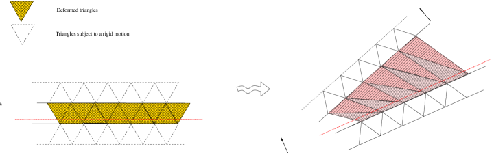
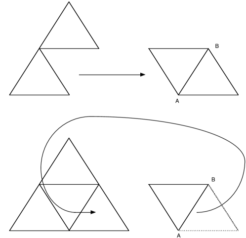
so that the energy density is always positive. As a first remark we will note that, using a result by Chambolle, Giacomini and Ponsiglione [14], gradients of limits of sequences with equi-bounded energy are piecewise rotations with an underlying partition of into sets of finite perimeter. This allows us to focus on the boundaries of such sets, where we have a normal on whose two sides we have the values of and two rotations among those labeling the sets of the partition. Note that from the standpoint of the microscopical triangulations the interfaces are the limits of triangles of side-length which are deformed by into triangles with one side (actually two) of diverging length but with the same ordering of the vertices (this corresponds to the positive-determinant constraint).

If only a layer of triangles is deformed that gives a limit interface, then this gives a relation between , and . In the simplest case when is orthogonal to one of the unit vectors of (we call those vectors coordinate normals), this relation reads as
This can be regarded as an opening-fracture condition in the “finite” case: note that in the “infinitesimal case” when is a small variation of a ground state; i.e., with , then this condition reduces to the usual infinitesimal crack-opening condition
since . If is not a coordinate normal then the opening-crack condition gets more complicated, due to microscopic anisotropies of the lattice, which disfavor cracks not orthogonal to lattice directions. The same anisotropies appear, as usual for lattice systems, in the form of the surface energy density. However, the situation described above is not the only possibility, since more than one layer of triangles may be “strongly deformed”. This gives a higher energy on the interface, but relaxes the constraints on , and . Moreover, additional energy contributions may be given by points where three or more interfaces meet; in this case, even though the opening-fracture condition above may be satisfied on each interface, the system of interfaces may be incompatible with the positive-determinant condition in their common point. It must be observed that by introducing an high number of extra interfaces at the discrete level, the finite opening-fracture condition can be removed altogether, at the expenses of a complex non-local form of the final energy.
We finally note that, even when non-local effects are neglected, the fracture energy density depends not only on the crack orientation and the crack opening , but also on the image of the crack in the deformed configuration, described by the tangential derivatives of on both sides of the crack. Such types of energies seem to be of interest in themselves, and the corresponding analytical techniques still relatively undeveloped (see [3]).
1 Some notation and preliminary results
In the sequel we denote by the scalar product in and with the usual euclidean norm, both for vectors in and matrices in , the meaning being clarified by the context. Moreover we will also use the symbol to denote the duality pair for and . For every , denotes the segment joining and .
The functional space involved in our discrete-to-continuous analysis will consist of measurable vector-valued functions whose components are special functions with bounded variation. Such functions are commonly used in the variational theories of Fracture (see e.g. the seminal paper by Francfort and Marigo [16], the book by Bourdin, Francfort and Marigo [5] and the review paper [2]).
Definition 1.1.
Given a fixed bounded open set, a function is a function with bounded variation in , denoted by , if its distributional derivative is a vector-valued Radon measure on .
We say that is a special function with bounded variation in , and we write , if and its distributional derivative can be represented on any Borel set as
for a countably -rectifiable set in that coincides -almost everywhere with the complement in of the Lebesgue points of . Moreover, is the approximate gradient of at , is a unit normal to , defined for -almost every , and are the traces of on both sides of (according to the choice of ). Here the symbol stands for the tensorial product of vectors; i.e., for any .
For fine properties of and functions and a rigorous definition of all the quantities introduced above we refer to [4], Ch. 4. SBV functions enjoy a good compactness property that here is stated in its simplest form, suited for our functionals.
Theorem 1.2.
Let be satisfying
| (1.1) |
for some . Then there exist a subsequence and a function such that in measure. In addition and weakly* as measures.
As a consequence we easily get that the limit function in the previous theorem has the further property that .
Moreover estimate (1.1) allows to discuss separately the lower semicontinuity of suitable bulk and surface integral involving, respectively, the absolutely continuous and jump part of the generalized distributional derivative.
In order to treat lower semicontinuous bulk integrals in the vectorial setting it is necessary to recall the notion of quasiconvexity and quasiconvex envelopes.
Definition 1.3.
We say that a lower-semicontinuous integrand is quasiconvex if
for every and . In addition, for any , the quasiconvex envelope of is defined as
In case is real valued and continuous one can give a precise description of its quasiconvex envelope.
Proposition 1.4.
Let be continuous. Then
| (1.2) |
for .
The following theorem deals with lower semicontinuity along sequences of SBV functions weakly converging [4].
Theorem 1.5.
Let be satisfying
| (1.3) |
for . If in measure, then . Moreover, for every quasiconvex integrand such that
for every and a positive constant, and for any norm in ,
there holds
| (1.4) |
The final tool we present is a ‘slicing result’ that allows to treat -dimensional energies by reducing to -dimensional ones [4].
Before entering into details we introduce some notation. For let be the line through the origin orthogonal to . If and we set
| (1.5) |
Moreover, if we define the function by
| (1.6) |
Theorem 1.6.
(a) Let . Then, for all the function belongs to for -almost every . Moreover for such we have
according to the cases or (the case being negligible) and for all Borel functions
(b) Conversely, if and, for all and for -almost every , with
then .
We introduce now a generalization of a rigidity type result in the SBV setting due to Chambolle, Giacomini, Ponsiglione (see [14]). Before going through the statement we need some preliminary definitions. First we recall the notion of Caccioppoli partition of a domain (see e.g. [15]).
Definition 1.7.
We say that a collection of pairwise disjoint measurable sets is a Caccioppoli partition of if and
Moreover, given any rectifiable set we say that a Caccioppoli partition of is subordinated to if .
The following result is the -dimensional version of the one contained in [14].
Theorem 1.8.
Let with and for almost every . Then there exists a Caccioppoli partition of subordinated to such that for almost every
where and .
2 Formulation of the problem
In the sequel will be any open bounded open set in . With fixed discretization step the reference lattice is given by where . We introduce also the following notations
Note that S is the set of unitary vectors in the lattice and for each is the set of its nearest neighbours.
We define also the set D of coordinate directions as
Dropping the dependence on whenever no confusion may arise we will use the symbol T to denote any triangle with vertices in and sides of length and will denote the sets of all such triangles. As already pointed out in the Introduction the choice of the lattice relies on the fact that is the simplest Bravais lattice in dimension compatible with a Cauchy-Born hypothesis. Before introducing the precise definition of the functionals object of our analysis we list here some notation used in the following sections for sets of indices or triangles:
where the symbol stands for the standard lexicographic order in . Thanks to this choice any pair of nearest-neighbouring indices is counted only once in the energy contribution.
With this notation given a discrete vector-valued displacement we consider its associated energy
where is a continuous function satisfying the following structure properties:
-
(i)
;
-
(ii)
;
-
(iii)
;
-
(iv)
for any such that for .
In what follows for the sake of computational simplicity we simply assume . Clearly, up to a scaling argument, the analysis remains valid for the general case.
As customary, in order to pass from discrete systems to a continuum formulation, it is convenient to identify a function with an element of .
Definition 2.1 (interpolation).
Given a discrete vector-valued function we define its interpolation in the whole as a function coinciding on each triangle with the linear interpolation of the values in its vertices.
Note that an interpolation is not uniquely defined on triangles close to . This will not affect our arguments since convergences are always considered in the interior of . We will identify a discrete function with its interpolation and maintain the same notation for both the discrete and continuous version, the notation being clarified by the context.
Remark 2.2.
In this setting another common procedure is to identify a discrete function with a piecewise-constant element in by assigning constant value on the cell , . In fact, none of the results stated in the following would be affected by this choice (see the discussion contained in [1]). Considering discrete functions as continuous piecewise-affine ones allows us to formulate the orientation preserving constraint in terms of the standard determinant of .
We are now able to introduce the class of admissible functions; i.e., a proper class of vector-valued functions on the lattice that are orientation preserving:
Finally, we define the functional on as
| (2.1) |
Remark 2.3.
Note that energies defined in (2.1) account only for interactions well contained in and the orientation-preserving constraint is not imposed a priori on an affine extension of u on the triangles intersecting . Actually, if one is interested in minimum problems endowed with boundary conditions (together with some perturbation or fidelity terms), a standard procedure in the framework of -convergence is to focus on the ‘principal’ part of the total energy, neglecting at first boundary data. Once this task is accomplished one can further deal with the initial problems up to modifying the limit energy according to the contribution arising from recovery sequences with correct boundary datum.
To proceed further with our analysis we need to fix a convergence on .
Definition 2.4 (discrete-to-continuum convergence).
According to the our identification of discrete functions with interpolations, given we say that , and we write simply , if we have and .
3 Compactness and a lower bound
In this section we first provide a description of the domain of any -limit functional of the discrete energies defined in (2.1). As already mentioned in the Introduction this space consists of piecewise rigid deformations with finite crack energy in the sense of Griffith’s theory; i.e., .
As a second result we exploit geometric measure theory techniques to establish a lower-bound estimate for the - without imposing any a-priori hypothesis on the deformation . Note that in the next section this bound will be proved to be optimal for the class of piecewise rigid deformations ‘with opening fracture’ in the sense of the anisotropies of the reference lattice. For such deformations the limit fracture energy is simply governed by an anisotropic Griffith-type energy density which reflects the anisotropies of the underlying triangular lattice.
Proposition 3.1.
Let be such that and
| (3.1) |
Then there exists a Borel function such that, up to subsequences, in . Moreover,
-
(i)
(finite Griffith fracture energy) with ;
-
(ii)
(piecewise rigidity) there exists a Caccioppoli partition subordinated to such that for almost every we have for suitable and .
Proof.
As a first step we observe that any pair belongs to two different triangles having the segment as a side. Hence if we take into account a factor we may estimate the energies from below with the integral functionals obtained as a superposition of gradient energies indexed by the triangles varying in . Actually, for any open set compactly supported in and for any , we have
| (3.2) | |||||
According to this standpoint, we are led to considering integral functionals with energy density . Hence, with fixed any we distinguish ‘good’ or ‘bad’ triangles depending whether the triangle energy overcomes the threshold or not. Using a standard separation of scales (see [8]) we set
and define as
| (3.3) |
with denoting the identity deformation. By construction the sequence lies in and for any its jump set is contained in the boundary of the union of the triangles in .
Moreover, for any open set compactly supported in inequality (3.2) can be rewritten in terms of as
| (3.4) |
for a positive constant . This implies at once that the functions and differ in a set of vanishing Lebesgue measure so that it is enough to prove that is compact in .
Thanks to hypothesis on the set
is a compact set in and this easily provides the estimate
On the other hand hypothesis ensures that there exists a constant such that (3.4) can be further sharpened as
| (3.5) |
Arguing by polar decomposition we also deduce that for any there exists such that , thus
| (3.6) |
Taking into account hypothesis (3.1) a straightforward application of Theorem 1.2, and the convergence to of , yields that there exists with such that in .
To prove we take advantage of a relaxation argument together with some rigidity estimates. Indeed, as a first step we prove that for almost every . To this end denote and estimate the right-hand side of (3.6) as
| (3.7) |
Passing to the liminf and using (1.4) we get at once that
Hence almost everywhere in and by applying Lemma 3.3 with we also get that the approximate gradient is a rotation for almost every . Once this fact is established follows by applying Theorem 1.8 recursively to with replaced by any open set compactly supported in and then letting invading . ∎
Remark 3.2.
Hypothesis (3.1) is essential to deduce a compactness result for sequences equibounded in energy and avoids the un-physical situation of particles escaping to infinity (modelled by arbitrarily large translations).
The following lemma completes the proof of Proposition 3.1. This kind of results are widely used in variational problems involving crystal microstructures.
Lemma 3.3.
Let and let be such that . Then .
Proof.
For fixed, taking into account Proposition 1.4, let contained in be such that
Setting for almost every , we have
Hence it is not restrictive to assume that and weakly in and , respectively. By lower semicontinuity, using that , we also get
Thus for almost every and the claim follows from the classical rigidity theorem in and the fact that . ∎
We underline that in the proof of Proposition 3.1 any choice of the parameter ensures the validity of estimate (3.7). Moreover, assuming that converges to a given in , any sequence , defined in (3.3), still converges to weakly in and the energy contribution is proportional to . Since is a sequence of rectifiable sets with normal coordinates this suggests that in the passage to the liminf on on the surface part of the right-hand side of (3.7) we may obtain a lower bound with a surface-type energy maintaining the simmetries of the hexagonal lattice. In the sequel we built the right surface energy arguing by pairwise interactions along lattice directions and exploiting more refined techniques in geometric measure theory.
Before entering into details we need to introduce some more tools. Let be the -homogeneous map such that coincides with the convex hull of the set S of the unitary vectors of the lattice and let its dual norm; i.e., is the polar function of defined as
An easy computation shows that
and is the -homogeneous functions whose unitary ball is the convex hull of the coordinate directions D scaled by a factor . In addition the following lemma holds true.
Lemma 3.4.
If is as above then for all .
Proof.
A direct computation shows that the inequality holds true as an equality for . Hence one can argue locally in each sector of amplitude by using the linearity of on such portions of and the result for the coordinate directions. The claim follows from the invariance of the inequality under rotations with angle . ∎
By means of Lemma 3.4 in the next proposition we will provide a lower bound on - of by a suitable anisotropic surface energy. Since by Proposition 3.1 the - of is finite only on we prove the estimate in that functional space.
Proposition 3.5.
Let , then for any it holds
| (3.8) |
Proof.
Let be fixed with in and . It is not restrictive to assume also that and almost everywhere in . Note that by Proposition 3.1 is a piecewise rigid deformation with .
We will proceed by a slicing technique, performed only in the lattice directions , in order to obtain the estimate
| (3.9) |
To this end we observe that we can split the energies by accounting separately the contribution of pairs with and letting varying in . Hence, setting for
we get
Thus it is enough to prove that for any
| (3.10) |
As the lattices and so the energies appearing in both sides of (3.10) are invariant under rotations of we confine our attention to prove (3.10) for and .
Note that the functionals consist of a superposition of -dimensional discrete energies related to the sublattices for even varying in and to the lattices for odd. Hence, as a first step we will use the usual separation of scales argument on these -dimensional discrete energies in order to rewrite them in a suitable -dimensional integral form and then we glue the information back to the -dimensional setting by a slicing procedure. More precisely, for any set
Note that the stripes give a partition of . For any we will construct a sequence with dimensional profile along the direction and depending only in the first variable in each stripe. Thus let be fixed and set
(for the sake of notation we drop the dependence on in what follows).
For any define on to be equal to the value on if and to be the affine interpolation of the values on any other interval . Eventually, extend on as .
Arguing as in the proof of Proposition 3.1 we infer that
| (3.11) |
and that in and, up to subsequences, also almost everywhere in . In addition
| (3.12) |
Taking into account that
and also that
for all , (3.12) can be rewritten as
| (3.13) |
By passing to the liminf in both sides of (3.13) and by applying Fatou’s Lemma we get
| (3.14) |
On the other hand, estimate (3.11) ensures that for -almost every the sequence is precompact in and converges in measure to . Hence by the -dimensional analogue of the lower semicontinuity Theorem 1.5 we infer that
| (3.15) |
Moreover, thanks to Theorem 1.6(a) with , we have
| (3.16) |
Letting concludes the proof of claim (3.9). Eventually, Lemma 3.4 yields (3.8). ∎
4 Upper estimates for a class of “opening cracks”
In this section we show the optimality of the bound (3.8) provided in Proposition 3.5 for a class of functions with ‘opening cracks’ with respect to the anisotropies inherited by the lattice.
In the next section more complex geometries will be taken into account and the occurrence of different phenomena will be highlighted. Actually, the representation of the limit energy seems to take into account several factors, not all of local nature.
In order to clarify the parameters playing a role in the asymptotic behaviour of , we prefer to deal with the case where only two rotations are involved in the target deformation first. In this setting the crack splits into two regions , in general not connected, each one underlying a rigid motion. We will show that in this case the -limsup of is finite even if the request of orientation-preserving recovery sequences affects substantially the form of the limit energy.
In this process a relevant condition that translates the positive-determinant constraint through the crack is the following:
| (4.1) |
In fact, the inequality above ensures that any small triangle crossing the fracture site maintains positive (non negative) area in the codomain. Actually, due to the discrete environment, condition (4.1) has to be assumed for , since the only triangles entering in the construction have sides parallel to the directions lying in S.
We start by proving the following characterization of the -limsup whenever is contained in a straight line and (4.1) holds.
Proposition 4.1.
For and with , let be defined as
| (4.2) |
Assume that and for -almost every satisfy the condition
| (4.3) |
then
| (4.4) |
Proof.
We claim that thanks to the hypothesis we may assume the stronger separation hypothesis
| (4.5) |
for some fixed and for -almost every .
Indeed, if (4.5) does not hold, it is enough to choose a vector such that (set for instance ) and consider the sequence defined replacing with in (4.2). Clearly in and the left-hand side term of (4.4) is continuous along such a sequence. Condition (4.5) plays a key role in showing that the sequence defined as the pointwise interpolation of in the nodes of the lattice is admissible and accounts for the desired -limsup estimate.
Thus, set for any . Clearly in ; it remains to check that the positive-determinant constraint is satisfied in any triangle contained in .
Before proceeding with the computation we label the triangles ‘crossing the fracture site’. By rotational and translational invariance we may assume so that . Let and set
and
Note that coincides with a ‘positive’ rotation on the vertices of those triangles not contained in the strip
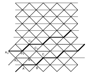
Hence, in order to ensure that , it suffices to check condition (4.3) for triangles T with vertices respectively and (see Fig. 2). This leads to prove the following inequalities:
for . These can be compactly rewritten as
| (4.6) |
We claim that these conditions are fulfilled for small enough. Indeed, for any infinite collection of indices with , up to subsequences, we may assume that as . As a consequence and , with . Thus, assuming that (4.6) are violated for such a sequence of indices will lead to a contradiction to (4.5) when passing to the limit as .
Eventually we compute the asymptotic value of to show that is a recovery sequence for the surface energy . Clearly, the energy contribution in reduces to those pairs of indices one of which of type with ; i.e.,
| (4.7) | |||||
Passing to the limit as and plugging the equality
in (4.7) the conclusion is achieved. ∎
The next proposition generalizes the result of Proposition 4.1 in the case when only two rotations are involved in the deformation and consists of segments having normals in D.
Proposition 4.2.
Let and be given with . Let be a connected union of segments with normal belonging to D and let
where is a Caccioppoli partition subordinated to . Assume that for -almost every it holds
| (4.8) |
then
| (4.9) |
Proof.
Up to an approximation argument we may assume that with for , having constant normal lying in D and satisfying for any . Thanks to the connectness hypothesis and to condition (4.8), arguing by perturbation with infinitesimal translations, condition (4.8) can be assumed to hold in the stronger form , for a positive . We claim that a recovery sequence is provided defining for . Indeed, for any triangle intersecting there exists a unique such that either is a single point in or for some . In both cases one may perform the same computation as in Proposition 4.1, and deduce that satisfies the positive-determinant constraint. Eventually a direct computation shows that . ∎
The previous approach can be pushed further to obtain the optimality of the bound (3.8) also for consisting of a line with normal . In this case we need to impose the opening crack condition (4.3) in a stronger sense; i.e., (4.3) must be satisfied also along the two directions generating in one of the simplex of the Wulff shape .
Proposition 4.3.
For and , let be defined as
| (4.10) |
Let be such that for . Assume that for -almost every satisfy the conditions
| (4.11) |
for and for some . Then
| (4.12) |
Proof.
The claim will be proved by an approximation argument, exploiting Proposition 4.2 and the lower semicontinuity of the -limsup. It is not restrictive to assume connected and with endpoints on . Note that hypothesis (4.11) ensures that . Let be a fixed small parameter and select a connected union of segments with normal equal to or to such that
| (4.13) |
and . By simply extending the polygonals above we may also assume that each has endpoints on and splits in two components such that
For let be the piecewise rigid function defined as
It is easily checked that in and, by continuity, satisfies hypothesis (4.11) with a smaller positive and replaced by . Applying Proposition 4.2 to each we get
The conclusion follows taking property (4.13) into account. ∎
In the following we consider the case in which the jump set consists in a triple point with coordinate normals.
Proposition 4.4.
Let be fixed and set
Let be defined as with for suitable and . Assume that satisfies the ‘opening crack’ conditions along :
| (4.14) |
and that satisfies the further compatibility condition
| (4.15) |
on the triple point . Then
| (4.16) |
Proof.
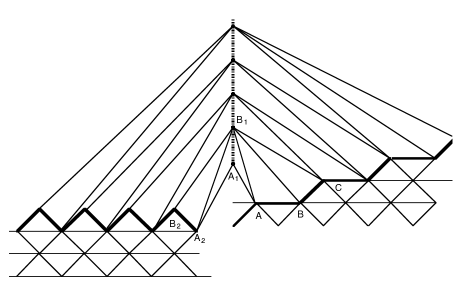
Up to composing with infinitesimal translations we may assume that, for any small enough, the points lie on the lattice . Set for any . Clearly in ; it remains to check that the positive-determinant constraint is satisfied in any triangle intersecting . Thanks to hypothesis (4.15) we have that there exists such that all the scalar products in (4.4) are greater than . By performing the same computation as in the proof of Proposition 4.1 we may deduce the positive-determinant constraint to be satisfied on any triangle intersecting and not containing . The only triangle left aside is then the one having vertices . A direct computation shows that
Hence the conclusion follows by hypothesis (4.15). ∎
As a conclusion of this section we note that we have proved that the -limit of is described by the anisotropic fracture energy
| (4.17) |
on all which are piecewise rigid deformations such that consists of a finite number of lines meeting at triple points and the opening-crack conditions in Proposition 4.4 are satisfied. This description extends by continuity to all piecewise rigid deformations that can be approximated in energy by sequences of piecewise rigid deformations satisfying such conditions.

5 Macroscopical failure of the positive-determinant constraint
In the previous sections we have computed the -limit of our discrete system when the macroscopic configuration satisfies compatibility conditions on the fracture site and at meeting points of three (or more) fracture sites. Those conditions can be regarded as a positive-determinant constraint on the fracture. In this section we will see how all those conditions can be removed. In this way macroscopic configurations “with negative-determinant fracture” can be obtained from atomistic configurations satisfying a microscopic positive-determinant constraint, at the expense of a strictly greater energy.

5.1 Removal of compatibility conditions on the fracture site – surface relaxation
The surface energy (4.17) has been obtained under a condition that implies that the fracture can be achieved by highly deforming only a single layer of positive-determinant triangles, keeping all other triangles at the minimum of the energy. We now show how, still using a single layer of triangles to create the fracture, we may relax conditions (4.11) in the case when .
We only illustrate the surface relaxation with an example. Consider a linear crack surface with normal , which does not belong to . In Fig. 4 we highlight a layer of triangles that may be used to obtain a fracture satisfying (4.11). If then the possible values for lie in the convex angle pictured on the right of the figure. We may obtain any with if we also deform the triangles neighbouring the ‘fracture layer’. A possible deformation is given in Fig. 5, where each such neighbouring triangle has one side compressed by a factor and one side compressed by a factor . This construction gives an estimate for the energy density on the fracture with
(while ).
Note that such a wide relaxation is not necessary for fixed , if . In general then, even in this simple geometry, we will obtain a surface energy density depending on .


5.2 Removal of compatibility conditions on the fracture site – multiple microfracture
By introducing more layers we may remove all constraints on , while the macroscopic energy varies by a factor proportional to the number of additional layers.
In Figure 6 the macroscopic deformation on the fracture does not satisfy the conditions
for the two “microscopic” coordinate normals . However, the discrete functions in the construction depicted in Figure 6 all have positive-determinant interpolations thanks to the introduction of a “fictitious” layer of atoms. In this case the limit energy per length doubles.
A variation of this example in given in Figures 7 and 8 to highlight that the introduction of an extra layer of atomic interactions allows to remove the condition even when is a coordinate normal. By repeating this process the macroscopic deformation may exhibit a interpenetration phenomenon.

Note that for some deformations surface relaxation may be energetically convenient with respect to multiple-layer fracture. This clearly is the case of the example in Section 5.1 when is close to satisfying the compatibility conditions (4.11).

5.3 Removal on compatibility conditions on “triple points” – micro-deformed fracture
The condition on triple points in the previous section ensures that the deformation of a microscopic triangle at that point is of positive determinant (and hence, being a single triangle, gives a negligible energy contribution). If such a condition does not hold then the use of (small variations of) pointwise interpolations on the different regions of the underlying partition is not possible, since for small there will always be a microscopic triangle whose vertices are mapped in three points which fail the positive-determinant constraint. However, it is possible to use a different interpolation by introducing an additional microscopic fracture enclosing small sets where the deformation is not in . Note that this is possible if such sets have the dimension of an interface.
In Figure 9 it is represented a deformation with a triple point failing the positive-determinant condition. In this case we introduce a microscopic approximation as represented in Figure 10.

On the fracture site we introduce a segment where the pointwise single-layer interpolation of the jump is substituted by a double-layer approximation. Note that the image of this segment undergoes an additional linear deformation. Note that the energy of this approximation provides the additional contribution
where the second term is due to the compression of the triangles on the segment in the reference configuration. This energy depends on the choice of and , which are variables in the construction (satisfying some constraints due to the positive-determinant requirement in the resulting construction). This shows that even in this simple case an optimization problems arises between the introduction of an additional microfracture and a microscopic compression. Of course, more complex constructions with more parameters can be also introduced.
5.4 Global failure of impenetrability constraints – optimal decomposition and healing microfractures
In the constructions illustrated above we could exhibit a microscopic recovery sequence by working separately on each fracture site or triple points. In the presence of a complex geometry of the domain, besides a use of those constructions one has also to take into account the possibility of introducing further “fictitious” microscopic interfaces to get around impenetrability constraints. As a simple example, we may consider the deformation in Figure 11,

where the central smaller triangle is removed and translated from its position in the larger triangle. This macroscopic deformation can be approximated by microscopic ones all satisfying the positive-determinant constraint (see Figure 12). One such approximation can be obtained by translating a rhombus and subsequently composing this translation with a deformation rotating half of this rhombus as described in Section 5.2 (see also Figure 8). Note that this last rotation entails the introduction of one or more microscopic fictitious layers of atoms.

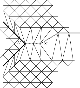
Another simple example is depicted in Figure 13, where the triangle to be removed is strictly contained in the interior of a larger triangle. In this case, in order to proceed as in the previous construction, one has to introduce an “auxiliary fracture” as the segment in the figure. The determination of the optimal shape and location of such auxiliary fracture sites is clearly a complex optimization problem. Note that in this case, also the determinant constraint for triple points has to be taken into account.
6 Necessary conditions for opening cracks
In Section 3 we have shown a lower bound with an anisotropic Griffith fracture energy, which is optimal on a family of displacements with an opening-crack condition on the fracture site (Section 4). We now show conversely that if the limit energy at a point is not greater than the lower bound then necessarily the function satisfies a opening-crack condition.
We now consider discontinuity points where the fracture energy density is minimal; i.e., the inequality in (3.8) is sharp, and derive necessary conditions on the crack opening. To this end we introduce the measures
| (6.1) |
These measures are nothing else than a way to measure locally the energy . If is a bounded sequence of measures and , then, arguing as in the proof of Proposition 3.1, we infer that is precompact in and that in . We also suppose that the weak∗ limit of exists.
Proposition 6.1 (necessity of an opening-crack condition).
Let , and let be such that
| (6.2) |
Then we have
| (6.3) |
where are the two constant matrices coinciding with on both sides of at .
Proof.
For the sake of brevity we will denote .
Let be a square centered in , with side length and an edge orthogonal to . With fixed and , let
which, by definition of converges as and to the function
By the weak∗ convergence of and (6.2) we deduce that
where is a cube centered in , with side length and an edge orthogonal to , and and are infinitesimal as and , respectively.
We fix and set
We claim that we may connect the two opposite sides of parallel to with a path (depending on and , but we omit such a dependence for the sake of notational simplicity) consisting of triangles such that and have a common side and up to a number of indices that is . Indeed, note that for any we have
| (6.4) |
If no path as above exists then we may construct disjoint paths in ; i.e., sets of indices with and , such that
and
| (6.5) |
(for a construction of such paths we refer to the proof of Theorem 4(ii) in [10]). Since converge to close two opposite sides of it is not restrictive to suppose that
By (6.5) we have
| (6.6) | |||||
Dividing by and letting and tend to we then obtain , which gives a contradiction.
We consider the connected set
Note that by the convergence , for all the set will be contained in the strip for sufficiently small. It is not restrictive to suppose that is composed exactly of two polygonal chains and . Note that the set
still gives a path with the same properties of . We can therefore suppose that this is our original path.
The contribution of the energy restricted to interactions in gives
| (6.7) |
(see Proposition 3.5). We then deduce that
| (6.8) |
and, in addition, there exist disjoint polygonal chains joining and the side of lying on such that they do not intersect . Since , arguing as in (6.6), we deduce that
| (6.9) |
as .
For fixed we may now consider the scaled functions
We may still argue as in Proposition 3.1 and deduce that converge to . Note that .
For fixed , we may now consider the functions
which are now discontinuous at . They satisfy
(i) the determinant of is equibounded, by the definition of ;
(ii) are equibounded;
(iii) is bounded;
(iv) the measures are equibounded, by (ii) and since by definition. Here and below we simply denote by the normal to a discontinuity set without specifying of which function, which is clear from the context.
By Theorem 5.8 in [3] from (i)–(iv) above and the convergence we deduce that the measures converge to . We choose the orientation of so that the determinant constraint on can be rewritten on each segment of as
where and are the values on two vertices of the corresponding triangle, with and . We then have, by (6.9)
Dividing by and letting we obtain the first claim in (6.3). The analogous inequality with is obtained in the same way.∎
Remark 6.2 (conjecture).
We have obtained a weaker necessary condition than the sufficient ones in (4.11). We conjecture that this is only a technical issue and indeed those condition are also necessary in order that the energy density be minimal on .
7 Small deformations
In the previous sections we have showed how the “positive-determinant” constraint on the fracture is not closed, and must be substituted by complex non-local energetic considerations. The constraint simplifies in the case of small deformations; i.e., if we require that
| (7.1) |
(or any function with gradient in in place of the identity) with .
If then we can still apply the compactness argument as above to obtain, from the boundedness of , that determines a partition into sets of finite perimeter. Since and , in the case of a single coordinate normal the constraint on
can be translated into one on that reads
| (7.2) |
(in the case of a general non-coordinate normal we have to take into account the microscopic oscillations of as usual). Note that this is the usual infinitesimal opening fracture constraint, which is a closed constraint.
Remark 7.1 (linearized regime).
The case of the order of corresponds to the one studied by Braides, Lew and Ortiz in the one-dimensional case when bulk and surface terms have the same scaling. Hence, the compactness argument used above does not hold, and the limit energy possesses both a bulk and a surface term. The linearization of the bulk term has been studied by Braides, Solci and Vitali [12], and can be used together with the analysis above. The resulting -limit can be explicitly written as
on piecewise functions whose discontinuity set is a union of smooth lines, satisfies the infinitesimal opening fracture constraint on . Note that a construction as in Section 5.3 implies that the condition on triple points can be dropped altogether (since microfractures can be chosen vanishing with ). The proof of the upper bound for the -limit is a technically complex matter due to the lack of density theorems for satisfying the resulting constraints, and will not be addressed here. Related results can be found in works by Friedrich and Schmidt [18, 19, 20, 17].
8 Conclusions
We have examined a two-dimensional system of nearest-neighbour interactions for Lennard Jones pair interactions parameterized on a triangular lattice, with a microscopic positive-determinant constraint which mimics the effect of long-range interactions and limits the ground states to rotations. The goal is to exhibit a continuum approximation so as to test the validity of such a simplified model.
In parallel to the one-dimensional case we have focused our attention on the fracture term of the resulting continuum approximation by suitably scaling the energies. We have thus determined
a surface energy density which reflects the triangular symmetries of the underlying lattice;
conditions on the interface that reflect the positive-determinant constraint. The conditions on the interfaces are of a novel type that take into account both the gradient of the deformation on both sides of the fracture and the orientation of the fracture site in the reference configuration. In addition we also have a positive-determinant constraint on points where more fracture meet (triple points);
such conditions are not a closed constraint, and can be removed by adding “fictitious” micro-fractures. The optimal location and form of those micro-fractures depends on the corresponding macroscopic deformation, and is a complex optimization problem;
in the case of small deformations the conditions on the interfaces reduce to the infinitesimal opening fracture constraint, which actually suggests a linearized approximation in the spirit of Braides, Lew and Ortiz with that constraint on the fracture (also analyzed in recent works by Friedrich and Schmidt [18, 19, 20, 17]).
We have neglected interactions other than nearest neighbours. In this way the interfacial energy does not reflect the possibility of surface relaxation; i.e., the fact that atomistic interactions are unbalanced close to interfaces. This is an important effect, especially at the boundary of the domain and in the determination of the location of fractures. It has been partially addressed by Theil [23], and should be included in further investigations on the subject. The one-dimensional analysis by Braides and Solci [11] suggests that considering longer range of interactions (e.g., next-to-nearest neighbours) could be used in the place of the determinant constraint in order to eliminate non-local effects for non-opening cracks, at the expense of introducing internal and external boundary layers.
Appendix: positive vs non-negative determinant constraint
We have considered a strictly positive microscopic determinant constraint. Strictly positive inequalities are weakened in the limit; however, our choice of not directly considering weak inequalities allows to rule out some additional “unphysical” deformations which would have to be taken into account by directly considering a non-negative microscopic determinant constraint. This would correspond to allowing microscopic interpolations to “collapse” triangles to segments on the jump set even though such collapsed triangles cannot be viewed as a limit for the strictly positive determinant case. This may happen in the case of rotations on both sides of the interface with .


In Fig. 14 we depict such a microscopic deformation along a single coordinate line, where all points of two rows are aligned. Note that allowing zero-determinant deformations would include such a macroscopic deformation in the set of “minimal interfacial energy”, while in our setting the same must be achieved by the introduction of at least one extra layer of atoms, thus doubling the energy.
Another possibility for having is with the partition composed of a pair of supplementary angles as in Figure 15. In this case it is possible to “rotate” one of the two angles by with positive or zero determinant on the deformed triangles along the discontinuity set. In both cases, however, we have a macroscopical failure of impenetrability, so we have regarded these cases as degenerate by considering only the strictly-positive-determinant constraint.


References
- [1] R. Alicandro, M. Focardi, and M.S. Gelli. Finite-difference approximation of energies in fracture mechanics, Ann. Scuola Norm. Sup. Pisa Cl. Sci. (4) 29 (2000), 671–709.
- [2] L. Ambrosio and A. Braides. Energies in SBV and variational models in fracture mechanics. In Homogenization and applications to material sciences (Nice, 1995) GAKUTO Internat. Ser. Math. Sci. Appl. 9, 1–22.
- [3] L. Ambrosio, A. Braides and A. Garroni. Special functions with bounded variation and with weakly differentiable traces on the jump set. Unpublished manuscript. Available at cvgmt.sns.it. Extended version of a paper appeared in Nonlinear Diff. Equations Appl. 5 (1998), 219–243
- [4] L. Ambrosio, N. Fusco, and D. Pallara. “Functions of Bounded Variation and Free Discontinuity Problems”, Oxford University Press, Oxford, 2000.
- [5] B. Bourdin, G.A. Francfort, and J.-J. Marigo. The Variational Approach to Fracture. Journal of Elasticity 91 (2008), 5–148,
- [6] A. Braides. -convergence for Beginners. Oxford University Press, Oxford, 2002.
- [7] A. Braides. Local minimization, variational evolution and -convergence. Lecture Notes in Math. 2094, Springer Verlag, Berlin, 2013.
- [8] A. Braides and M.S. Gelli. Limits of discrete systems without convexity hypotheses. Math. Mech. Solids 7 (2002), 41–66.
- [9] A. Braides, A. Lew and M. Ortiz. Effective cohesive behaviour of layers of interatomic planes. Arch. Ration. Mech. Anal. 180 (2006), 151–182.
- [10] A. Braides and A. Piatnitski. Overall properties of a discrete membrane with randomly distributed defects. Arch. Ration. Mech. Anal., 189 (2008), 301–323
- [11] A. Braides and M. Solci. Asymptotic analysis of Lennard-Jones systems beyond the nearest-neighbour setting: A one-dimensional prototypical case. Math. Mech. Solids, to appear, doi: 10.1177/1081286514544780
- [12] A. Braides, M. Solci, and E. Vitali. A derivation of linear elastic energies from pair-interaction atomistic systems. Netw. Heterog. Media 2 (2007), 551–567.
- [13] A. Braides and L. Truskinovsky. Asymptotic expansions by Gamma-convergence. Cont. Mech. Therm. 20 (2008), 21–62
- [14] A. Chambolle, A. Giacomini and M. Ponsiglione. Piecewise rigidity. J. Funct. Anal. 244 (2007), 134–153.
- [15] G. Congedo and I. Tamanini. Problemi di partizioni ottimali con dati illimitati. Atti Accad. Naz. Lincei Cl. Sci. Fis. Mat. Natur. Rend. Lincei (9) Mat. Appl., 4 (1993), 103–108.
- [16] G.A. Francfort and J-J. Marigo. Revisiting brittle fracture as an energy minimization problem. J. Mech. Phys. Solids 46 (1998), 1319–1342.
- [17] M. Friedrich, A derivation of linearized Griffith energies from nonlinear models. Preprint 2015.
- [18] M. Friedrich, B. Schmidt. An atomistic-to-continuum analysis of crystal cleavage in a two-dimensional model problem. J. Nonlinear Sci. 24 (2014), 145–183
- [19] M. Friedrich, B. Schmidt. On a discrete-to-continuum convergence result for a two dimensional brittle material in the small displacement regime. Netw. Heterog. Media 10 (2015), 321–342
- [20] M. Friedrich, B. Schmidt. An analysis of crystal cleavage in the passage from atomistic models to continuum theory. Arch. Ration. Mech. Anal. 217 (2015), 263–308
- [21] G. Friesecke, F. Theil. Validity and failure of the Cauchy-Born hypothesis in a two-dimensional mass-spring lattice. J. Nonlinear Sci. 12 (2002), 445–478.
- [22] A. Theil. A proof of crystallization in two dimensions. Comm. Math. Phys. 262 (2006), 209-236.
- [23] A. Theil. Surface energies in a two-dimensional mass-spring model for crystals. ESAIM Math. Model. Numer. Anal. 45 (2011), 873–899.
- [24] L. Truskinovsky, Fracture as a phase transition, Contemporary research in the mechanics and mathematics of materials (R.C. Batra and M.F. Beatty eds.) CIMNE, Barcelona, 1996, 322-332.