Wave mechanics in media pinned at Bravais lattice points

Abstract

The propagation of waves through microstructured media with periodically arranged inclusions has applications in many areas of physics and engineering, stretching from photonic crystals through to seismic metamaterials. In the high-frequency regime, modelling such behaviour is complicated by multiple scattering of the resulting short waves between the inclusions. Our aim is to develop an asymptotic theory for modelling systems with arbitrarily-shaped inclusions located on general Bravais lattices. We then consider the limit of point-like inclusions, the advantage being that exact solutions can be obtained using Fourier methods, and go on to derive effective medium equations using asymptotic analysis. This approach allows us to explore the underlying reasons for dynamic anisotropy, localisation of waves, and other properties typical of such systems, and in particular their dependence upon geometry. Solutions of the effective medium equations are compared with the exact solutions, shedding further light on the underlying physics. We focus on examples that exhibit dynamic anisotropy as these demonstrate the capability of the asymptotic theory to pick up detailed qualitative and quantitative features.

1 Introduction

The design of structures that have material properties that are controllable, or that do not naturally occur, is highly topical. It is now possible to talk of a negative refractive index, and to design materials accordingly in acoustics [15] and electromagnetism, or to design photonic crystals [26] whose overall properties are governed by their regular microstructure. Much of this literature draws upon earlier work in solid state physics [9, 29].

For design purposes, the arrangement of inclusions in hexagonal or rhombic patterns is typical in photonic crystals [43]. This special subset can be distinguished from the remaining oblique planar geometries by the symmetries of their first Brillouin zones (see section 2), and together with these, and two distinct orthogonal lattices, they form the set of two-dimensional Bravais lattices [9] as shown in Fig. 1. Notably, a honeycomb array is simply a hexagonal array with two pins per elementary cell so we can, and do, consider this case too due to the remarkable properties of graphene [37].

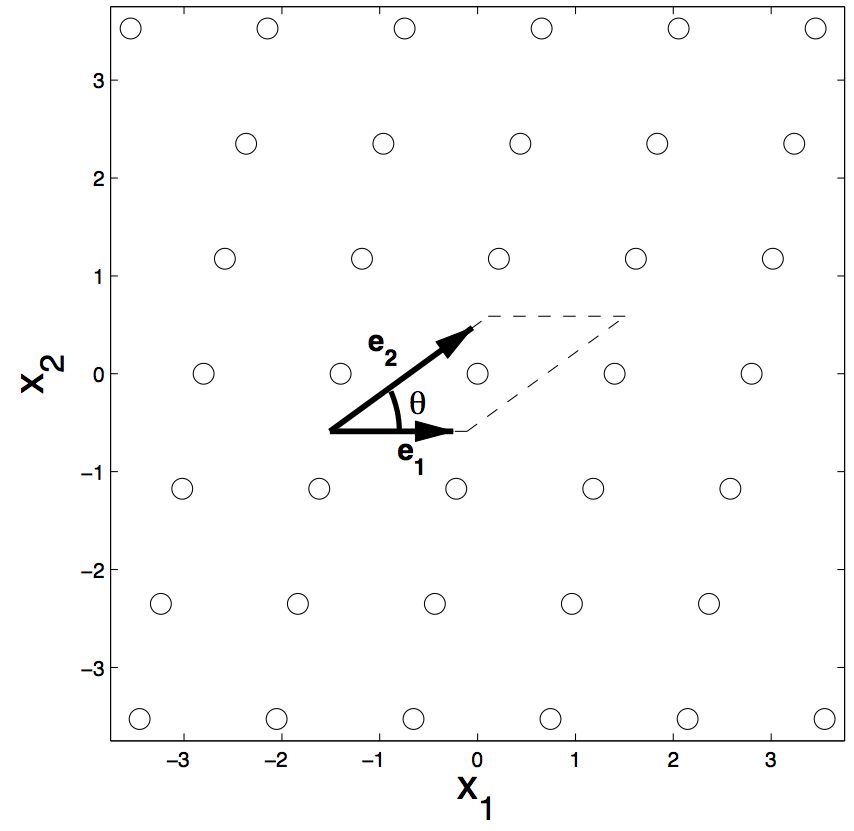
(a) Oblique

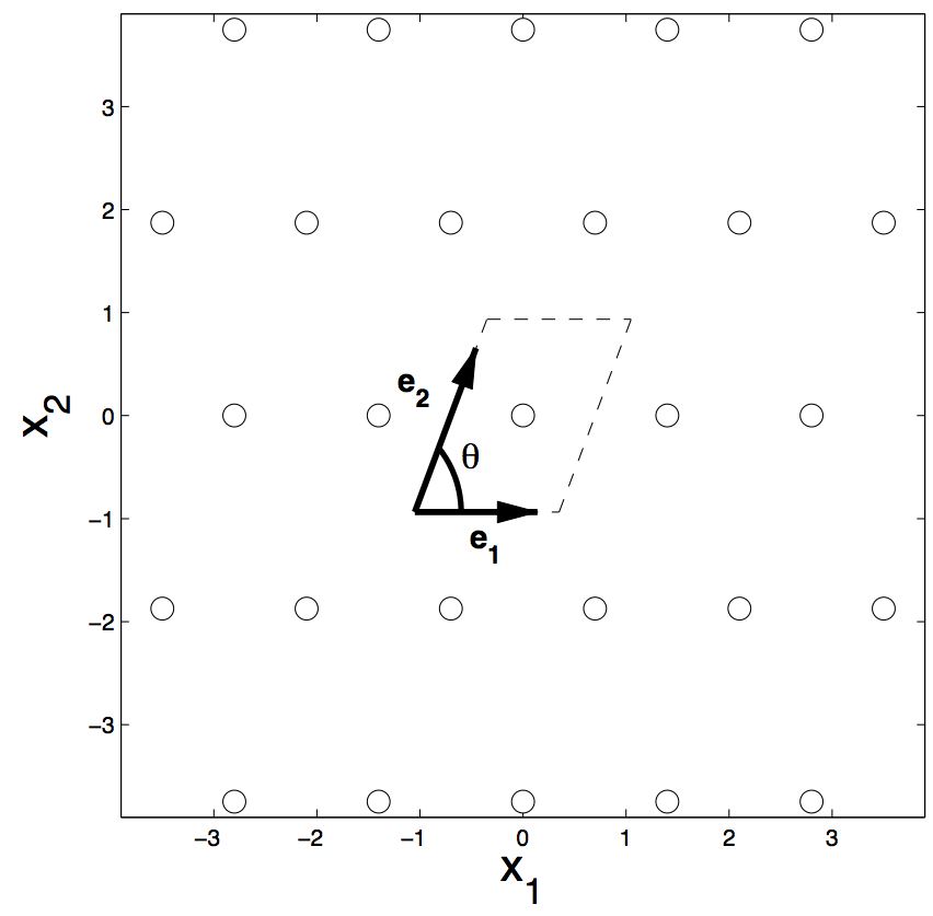
(b) Rhombic

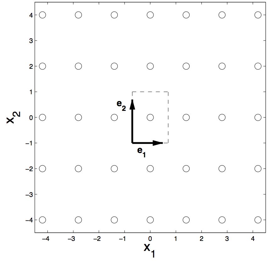
(c) Rectangular

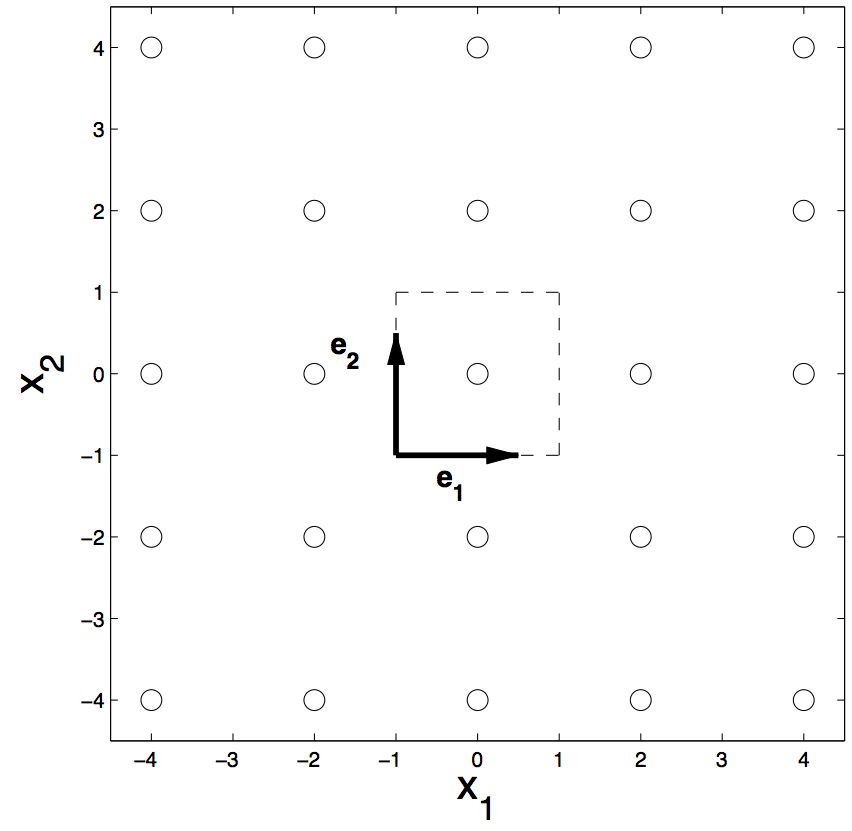
(d) Square

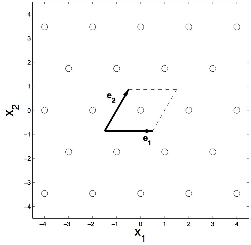
(e) Hexagon

Fig. 1: Illustrations of the 5 Bravais lattices together with their associated lattice basis vectors.

Our approach is to consider two distinct systems in this paper; physically the Helmholtz equation

(1) $$\nabla_{{\bf x}}\cdot\left[\hat{a}\left({\bf x}\right)\nabla_{{\bf x}}u({\bf x})\right]+\hat{\rho}\left({\bf x}\right)\Omega^{2}u({\bf x})=0$$

can be used to model transverse electric (TE) or transverse magnetic (TM) polarised electromagnetic waves, shear horizontal (SH) polarised elastic waves and pressure waves in the frequency domain. The spatially-dependent physical parameters $\hat{a}({\bf x})$, $\hat{\rho}({\bf x})$ will be assumed periodic in space, and represent different quantities depending on the physical setting, for example stiffness and density in the SH elastic system. We consider structures containing arbitrarily shaped inclusions and provide Dirichlet conditions on their boundaries, and later take the zero radius limit to point scatterers. There is wide interest in similar continuum problems; for instance [41, 42] provide typical applications for rhombic lattice arrangements.

A system closely related to the one described above is that of a structured elastic plate governed by the Kirchhoff-Love equation, for which vertical displacements satisfy

(2) $$\nabla_{\bf x}^{2}\left[\beta\left({\bf x}\right)\nabla_{\bf x}^{2}u\left({\bf x}\right)\right]-\mu\left({\bf x}\right){\hat{\Omega}}^{2}u\left({\bf x}\right)=0.$$

The non-dimensional squared frequency is

(3) $$\hat{\Omega}^{2}=\frac{\rho_{0}A_{0}l^{4}\Omega^{2}}{E_{0}I_{0}},$$

where the quantities appearing above are reference values of density, cross-sectional area, Young’s modulus and cross-section moment of inertia, related to the (spatially varying) values in the plate via the relations $EI=E_{0}I_{0}\beta\left({\bf x}\right),\rho A=\rho_{0}A_{0}\mu\left({\bf x}\right)$. The dimensionless quantities $\beta$ and $\mu$ thus represent the non-dimensional mass per unit length and flexural rigidity of the plate respectively. There has been considerable interest in such systems as platonic crystals, in which ideas from photonic crystals are transplanted into this setting [3, 10, 18, 20, 21, 34, 39, 40]. The additional derivatives in (2) compared to (1) lead to differences in the corresponding physical systems, but since the mathematics is closely related we choose to develop the theory for both equations in parallel. In the latter case we too shall study the zero-radius limit, noting that for an array of clamped pins there is a straightforward exact solution for a square array using Fourier series [2, 30, 31] that can be modified to other lattice arrangements [35]. Since points are the zero-radius limit of circular holes, one can also approach this problem using multipole methods [36], though we do not pursue this here. Additionally the stop band and localisation effects of plates containing an ordered arrangement of thin long fibres, which is reminiscent of clamped pins, has been studied experimentally [38].

Our primary aim is to generate homogenised, effective medium equations that capture the essential physics in a long-scale governing equation that encapsulates the short-scale structure in geometry-dependent coefficients. This is achieved using the multiple-scales methodology of high frequency homogenisation developed for square lattice structures in [17], and here generalised for Bravais lattices for which there are significant technical issues to overcome. The asymptotic methodology of [17] relies on perturbing away from solutions found at the edges of the Brillouin zone, though we demonstrate in section 2 that it can be applied at any point therein. The importance of band gap edges was recognised in the analysis community [7], as well as by those studying the high frequency long wave asymptotics of waveguides [24, 27, 28], a subject that has strong analogies to wave propagation in periodic media [16]. We note that the desire to obtain effective properties is not limited to systems governed by (1), (2) and also arises in studies of the Schrödinger equation [1, 25], in particular for potentials associated with honeycomb structures [22].

An additional aim here is to generate exact Fourier series solutions in the zero-radius limit of pinned points for both systems (1), (2). We then use these solutions to investigate the effectiveness of the asymptotic method, as well as the effects of geometry, and in particular lattice symmetries. In the case of the Kirchhoff-Love equation (2), this methodology applied to a square lattice gives effective medium equations [2] that predict and model shielding and lensing effects for elastic plates [3, 5]. Given this success for square arrays, and subsequent extensions to vector wave systems such as in-plane elasticity [4, 8], it is natural to extend the approach to Bravais lattice arrangements that are of broader physical interest.

The plan of the paper is as follows: in section 2 we introduce the mathematical description of the lattice geometries. With this background we then proceed, in section 3, to our two-scale analysis of the wave systems in question. The upshot in both cases is that a long-scale partial differential equation emerges with the short-scale and geometry built into a tensor of coefficients. Notably, although the governing equation (2) is fourth-order, the long-scale equation that emerges is typically of second-order. Situations whereby dispersion curves cross are not uncommon and often correspond to Dirac-like points that arise due to repeated eigenvalues; this is also incorporated into the asymptotic theory and described herein. Section 4 uses Fourier methods to construct exact solutions in the limit of point-like inclusions, which are used to provide checks on the asymptotic theory, as well as being interesting in their own right. These, together with the asymptotics, are used to interpret and model wave phenomena in section 5. The asymptotic theory clearly captures not just qualitative features, but also quantitative decay rates for localised states and the detailed dispersive properties near standing wave eigenfrequencies. Concluding remarks are drawn together in section 6.

2 Formulation

We consider a two-dimensional structure comprised of a doubly periodic array of cells. In our previous articles, inclusions were assumed to be arranged in a square geometry and our aim here is to create an asymptotic theory that is more general in terms of lattices, and to emphasise the differences between orthogonal and non-orthogonal geometries. We extend the existing methodology to deal with the $5$ fundamental two-dimensional Bravais lattices given by the crystallographic restriction theorem, as shown in Fig. 1. We allow for cases in which the cells contain $N\in\mathbb{N}$ inclusions, which is achieved by associating one or more inclusions to each lattice point.

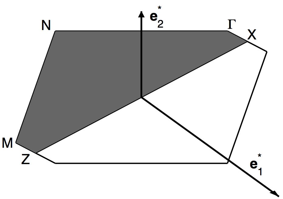
(a) Oblique

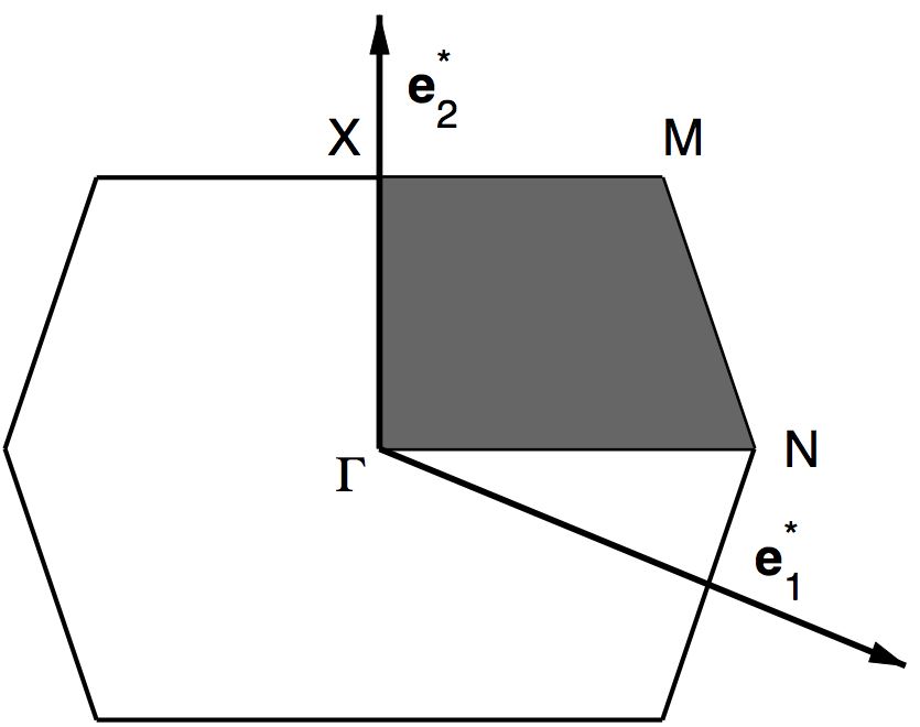
(b) Rhombic

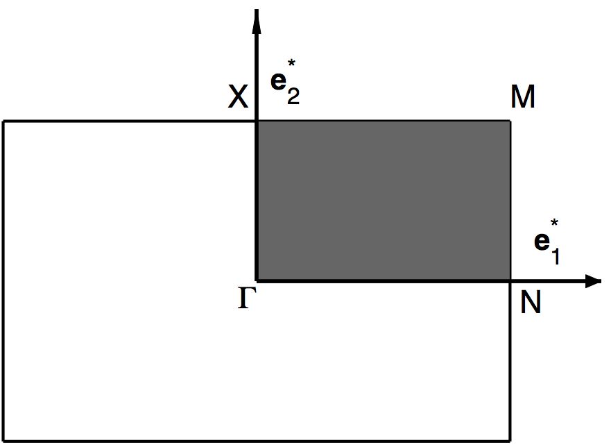
(c) Rectangular

(d) Square

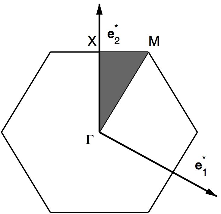
(e) Hexagon

Fig. 2: Illustrations of the first Brillouin zones for the 5 Bravais lattices. The shaded region shows the irreducible zone. Parameter values for each of the panels are (a) $\varphi(0.7,\pi/5)$   (b) $\varphi(0.7,\arccos(0.35))$   (c) $\varphi(0.7,\pi/2)$   (d) $\varphi(1,\pi/2)$  (e) $\varphi(1,\pi/3)$.

By definition, a Bravais lattice consists of an infinite array generated by a set of discrete translation vectors

(4) $${\bf R}=\sum\limits_{i=1}^{N}n_{i}{\bf e}_{i},\hskip 14.22636ptn_{i}\in\mathbb{N},$$

where ${\bf e}_{i}$ are the lattice basis vectors and $n_{i}$ are integer weighting functions. Consequently the medium appears identical when viewed from any unit cell. Generally, the primitive vectors defining a two-dimensional periodic lattice are written as

(5) $${\bf e}_{1}=\alpha A_{2D}{\bf i},\hskip 11.38092pt{\bf e}_{2}=A_{2D}\left[\cos\theta{\bf i}+\sin\theta{\bf j}\right],$$

where ${\bf i},{\bf j}$ are the unit orthogonal vectors, $\alpha$ is the asymmetry ratio, $A_{2D}\in\mathbb{R}$, and $0<\theta\leq\pi/2$. To obtain reciprocal lattice basis vectors, ${\bf e}_{i}^{*}$, we utilise the following orthogonality condition,

(6) $${\bf e}_{i}\cdot{\bf e}_{j}^{*}=2\pi\delta_{ij},\hskip 5.69046pti,j=1,2$$

to give us the reciprocal lattice basis vectors

(7) $${\bf e}_{1}^{*}=\frac{2\pi}{\alpha A_{2D}}\left[{\bf i}-\cot\theta{\bf j}\right],\hskip 11.38092pt{\bf e}_{2}^{*}=\frac{2\pi}{A_{2D}}\operatorname{cosec}\theta{\bf j}.$$

The non-dimensional position vector of any point in the medium is given by ${\bf r}=\xi_{1}{\bf i}+\xi_{2}{\bf j}=\zeta_{1}{\bf e}_{1}+\zeta_{2}{\bf e}_{2}$ and using this, along with equation (5), we deduce the following relations

(8) $$\xi_{1}=A_{2D}\left[\zeta_{1}\alpha+\zeta_{2}\cos\theta\right],\hskip 11.38092pt\xi_{2}=\zeta_{2}A_{2D}\sin\theta.$$

We denote the lattice satisfying equations (5)-(8) by the general function $\varphi(\alpha,\theta)$; this definition is sufficient as any two-dimensional lattice can be described by its asymmetry ratio and angular component. For example, the square lattice is denoted by $\varphi\left(1,\pi/2\right)$ and the remaining Bravais lattices are defined in table 1. Clearly, lattices (b) - (e) in Fig. 1 can be considered special cases of the oblique lattice (a), but a key distinction can be made by analysing the symmetries of the first Brillouin zones (Fig. 2); for oblique lattices that have parameter values $(\alpha,\theta)$ which do not coincide with those found in the $4$ distinguished lattices, there exists only a single line of symmetry bisecting the first Brillouin zone. This bears particular relevance to our analysis as the majority of features we are interested in, such as stop-bands, critical points and degeneracies, are captured by traversing along the boundary of the irreducible Brillouin zone. Notably one requires some care in doing so [14].

Topology	General function	Restrictions
Oblique	$\varphi\left(\alpha,\theta\right)$	$\alpha\neq 1,\theta\neq\pi/2$
Rhombic	$\varphi\left(\alpha,\arccos\left(\alpha/2\right)\right)$	$\alpha\neq 1$
Rectangle	$\varphi\left(\alpha,\pi/2\right)$	$\alpha\neq 1$
Square	$\varphi\left(1,\pi/2\right)$	-
Hexagonal	$\varphi\left(1,\pi/3\right)$	-

Table 1: The 5 fundamental Bravais lattices are defined in the above table. Definitions are given via the function $\varphi(\alpha,\theta)$, as any two-dimensional lattice can be uniquely defined by the angular component $\theta$ and asymmetry ratio $\alpha$.

The boundary of the first Brillouin zone, for all the geometries, is given by

(9) $${\bf G}\cdot\left({{\boldsymbol{\kappa}}}-\frac{{\bf G}}{2}\right)=0,\hskip 5.69046pt{\bf G}=m_{1}{\bf e}_{1}^{*}+m_{2}{\bf e}_{2}^{*},$$

where $m_{i}=(0,\pm 1)$. This definition allows us to find a general form for the edges of the irreducible zone, $\Gamma,X,M$ and $N$, for the rhombic, hexagonal and orthogonal geometries (fig. 2):

$$\Gamma=\left(0,0\right),\enskip X=\left(0,\pi\operatorname{cosec}(\theta)\right),$$

$$M=\left(\frac{\pi}{\alpha}\left[1+\cot(\theta)^{2}\right]-\pi\cot(\theta)\operatorname{cosec}(\theta),\pi\operatorname{cosec}(\theta)\right),$$

(10) $$N=\left(\frac{\pi}{\alpha}\left[1-\cot(\theta)^{2}\right]+\pi\cot(\theta)\operatorname{cosec}(\theta),\pi\left[\operatorname{cosec}(\theta)-\frac{2}{\alpha}\cot(\theta)\right]\right).$$

Given this geometrical set-up, and the relation to the reciprocal space, we now move on to the asymptotic procedure.

3 Asymptotic theory

In the following section we detail the generalised high frequency homogenisation method. Initially we consider the Helmholtz equation, before moving onto the case of platonic crystals governed by the Kirchhoff-Love equation.

3.1 Helmholtz equation

In this section we detail the asymptotic procedure as applied to the following governing equation:

(11) $$\nabla_{{\bf x}}\cdot\left[\hat{a}\left({\bf x}\right)\nabla_{{\bf x}}u({\bf x})\right]+\Omega^{2}\hat{\rho}\left({\bf x}\right)u({\bf x})=0.$$

Here ${{\bf x}}$ are the orthogonal coordinates on the infinite domain. The material is characterised by the periodic functions $\hat{a}\left({\bf x}\right),\hat{\rho}\left({\bf x}\right)$.

In the dimensional setting, the unit cell is taken to have sides of length $2\alpha l$ and $2l$ in the ${\bf e}_{1},{\bf e}_{2}$ directions respectively, where for convenience we also set $A_{2D}=1$ in equations (5). We begin to non-dimensionalise equation (11) by setting, $\hat{a}\equiv\hat{a}_{0}a({\bf x})$ and $\hat{\rho}\equiv\hat{\rho}_{0}\rho({\bf x})$ in (11):

(12) $$l^{2}\nabla_{{\bf x}}\cdot[a({\boldsymbol{\xi}})\nabla_{{\bf x}}u({\bf x})]+\Omega^{2}\rho({\boldsymbol{\xi}})u({\bf x})=0\quad{\rm with}\quad\Omega=\frac{\omega l}{\hat{c}_{0}}$$

and $\hat{c}_{0}=\sqrt{\hat{a}_{0}/\hat{\rho}_{0}}$.

We now introduce independent short- and long-scales $l$ and $L$, and the ratio of these two scales $\epsilon=l/L\ll 1$ will provide the small (positive) parameter, $\epsilon$, to be used further on in our homogenisation method. The two disparate length scales then motivate new sets of dimensionless coordinates, namely ${\bf X}={\bf x}/L$ and ${\boldsymbol{\xi}}={\bf x}/l$. We augment these with a third set ${\boldsymbol{\zeta}}$, which are related to ${\boldsymbol{\xi}}$ via the relations (8). It will be convenient to use the orthogonal short-scale ${\boldsymbol{\xi}}$ for asymptotic expansions of (11), and then revert to the lattice coordinates ${\boldsymbol{\zeta}}$ when we wish to impose the periodicity conditions and later for performing integrals over the cell. As is conventional in multiple scale analysis we treat ${\boldsymbol{\xi}},{\bf X}$ as being independent.

We proceed by placing the disparate orthogonal coordinates into (12), noting that the periodicity of the functions $a$ and $\rho$ is specified on the short-scale only:

$$\nabla_{{\boldsymbol{\xi}}}\cdot[a({\boldsymbol{\xi}})\nabla_{{\boldsymbol{\xi}}}u({\bf X},{\boldsymbol{\xi}})]+\Omega^{2}\rho({\boldsymbol{\xi}})u({\bf X},{\boldsymbol{\xi}})$$

(13) $$\qquad+\epsilon[2a({\boldsymbol{\xi}})\nabla_{\boldsymbol{\xi}}+\nabla_{{\boldsymbol{\xi}}}a({\boldsymbol{\xi}})]\cdot\nabla_{{\bf X}}u({\bf X},{\boldsymbol{\xi}})+\epsilon^{2}a({\boldsymbol{\xi}})\nabla^{2}_{\bf X}u({\bf X},{\boldsymbol{\xi}})=0.$$

Note that $u$ is now a function of independent separated-scale coordinates so $u=u({\bf X},{\boldsymbol{\xi}})$. Our focus will be on analysing the motion of the system near specified eigenfrequencies. An important point is that, dissimilar to orthogonal geometries, standing wave eigenmodes exist for non-orthogonal geometries that do not necessarily satisfy in-phase or out-of-phase boundary conditions at the edges of the cell. Notably for these eigenmodes the phase-shift across the cell is complex and this in turn gives rise to displacements having a non-zero imaginary component. As a result our asymptotic method is no longer restricted to dealing with real eigenmodes and we can analyse eigenfrequencies across the entirety of the Bloch spectrum and thereby perturb about any point in wavevector space. The Bloch conditions on the short-scale are applied using the general coordinates:

(14) $$u|_{\zeta_{i}=1}=\exp\left(2i{\boldsymbol{\kappa}}\cdot{\bf e}_{i}\right)u|_{\zeta_{i}=-1}\quad{\rm and}\quad u_{,\zeta_{i}}|_{\zeta_{j}=1}=\exp\left(2i{\boldsymbol{\kappa}}\cdot{\bf e}_{i}\right)u_{,\zeta_{i}}|_{\zeta_{j}=-1}$$

where $u_{,\zeta_{i}}$ denotes partial differentiation with respect to $\zeta_{i}$. We now take the following ansatz

(15) $$u({\bf X},{\boldsymbol{\xi}})=u_{0}({\bf X},{\boldsymbol{\xi}})+\epsilon u_{1}({\bf X},{\boldsymbol{\xi}})+\epsilon^{2}u_{2}({\bf X},{\boldsymbol{\xi}})+\ldots,\quad\Omega^{2}=\Omega_{0}^{2}+\epsilon\Omega_{1}^{2}+\epsilon^{2}\Omega_{2}^{2}+\ldots$$

which leads to a hierarchy of equations at different orders of $\epsilon$. The first three orders yield

(16a) $$(au_{0,\xi_{i}})_{,\xi_{i}}+\Omega_{0}^{2}\rho u_{0}=0$$

(16b) $$(au_{1,\xi_{i}})_{,\xi_{i}}+\Omega_{0}^{2}\rho u_{1}=-(2au_{0,\xi_{i}}+a_{,\xi_{i}}u_{0})_{,X_{i}}-\Omega_{1}^{2}\rho u_{0}$$

(16c) $$\begin{split}(au_{2,\xi_{i}})_{,\xi_{i}}+\Omega_{0}^{2}\rho u_{2}=-au_{0,X_{i}X_{i}}-(2au_{1,\xi_{i}}+a_{,\xi_{i}}u_{1})_{,X_{i}}\\ -\Omega_{1}^{2}\rho u_{1}-\Omega_{2}^{2}\rho u_{0}.\end{split}$$

For the leading order equation there is a solution precisely at $\Omega_{0}$ and a corresponding eigenmode $U_{0}({\boldsymbol{\xi}};\Omega_{0})=U_{0}({\boldsymbol{\zeta}};\Omega_{0})$, with a fixed phase shift in ${\boldsymbol{\zeta}}$,

(17) $$u_{0}({\bf X},{\boldsymbol{\xi}})=f_{0}({\bf X})U_{0}({\boldsymbol{\zeta}};\Omega_{0}),$$

where the the PDE governing $f_{0}({\bf X})$ is to be determined.

We now use the perturbation method about the frequency $\Omega_{0}$, and initially concentrate on the treatment of isolated eigenvalues. Repeated eigenvalues can and frequently do arise, and such cases require modifications. These cases are often associated with Dirac-like cones and will be dealt with later. We now assume that there are $N$ inclusions per unit cell, hence the total surface $S=S_{1}-\left(S_{2}\cup S_{3}\cup...\cup S_{N+1}\right)$, where $S_{1}$ denotes the surface of the unit cell without holes and $S_{j}$ ($j=2\rightarrow N+1$) represent the surfaces of the holes. We impose Dirichlet conditions on the boundaries $\partial S_{j}$ and deduce

(18) $$u({\bf X},{\boldsymbol{\zeta}})|_{\partial S_{j}}=0\iff u_{i}({\bf X},{\boldsymbol{\zeta}})|_{\partial S_{j}}=0,\quad i\in\ \mathbb{N}.$$

As these conditions are set in the short-scale ${\boldsymbol{\zeta}}$ we obtain for $i=0$, $U_{0}({\boldsymbol{\zeta}};\Omega_{0})|_{\partial S_{j}}=0$.

To proceed we apply the Fredholm alternative. We first multiply equation (16b) by $U_{0}^{*}$ and integrate over the cell’s surface:

$$\iint_{S}\left(U_{0}^{*}(au_{1,\xi_{i}})_{,\xi_{i}}+\Omega_{0}^{2}\rho U_{0}^{*}u_{1}\right)dS$$

(19) $$\qquad\qquad=-f_{0,X_{i}}\iint_{S}\left[(a|U_{0}|^{2})_{,\xi_{i}}+\beta_{i}\right]dS-f_{0}\Omega_{1}^{2}\iint_{S}\rho|U_{0}|^{2}dS,$$

(20) $$\text{where}\quad\beta_{i}=a\left[U_{0}^{*}U_{0,\xi_{i}}-U_{0}U_{0,\xi_{i}}^{*}\right],$$

and $|U_{0}|$ denotes the modulus of the complex displacement.

The first term on the right hand side of (19) vanishes when we use the planar divergence theorem along with the Bloch conditions (14) directed along ${\boldsymbol{\zeta}}$. We continue by subtracting the cell integral of the conjugated Helmholtz equation $(aU^{*}_{0,\xi_{i}})_{,\xi_{i}}+\rho\Omega_{0}^{2}U^{*}_{0}=0$ multiplied by $u_{1}$ to obtain:

(21) $$\iint\left[U_{0}^{*}(au_{1,\xi_{i}})_{,\xi_{i}}-u_{1}(aU_{0,\xi_{i}}^{*})_{,\xi_{i}}\right]dS=-f_{0,X_{i}}\iint\beta_{i}dS-f_{0}\Omega_{1}^{2}\iint\rho|U_{0}|^{2}dS.$$

Using Green’s theorem, the left side of equation (21) becomes

(22) $$\int a({\boldsymbol{\zeta}})\left(U_{0}^{*}\frac{\partial u_{1}}{\partial n}-u_{1}\frac{\partial U_{0}^{*}}{\partial n}\right)ds,$$

where the line integral in the first line is over $\partial S=\partial S_{1}\cup\partial S_{2}\cup\partial S_{3}...\cup\partial S_{N+1}$ and we have assumed that $\rho,a\in\mathbb{R}$. In equation (22) we find that by applying the Bloch conditions (14) the terms on the opposing boundaries of the cell cancel each other out, and with the help of the Dirichlet boundary conditions on the inclusions, the terms above go to zero. Hence we are left only with the terms on the right hand side of equation (21) and if the surface integral of $\beta_{i}\neq 0$ then we are left with a first-order governing equation for $f_{0}({\bf{X}})$:

(23) $$T_{i}^{(1)}f_{0,X_{i}}-\Omega_{1}^{2}f_{0}=0,\quad T_{i}^{(1)}=\frac{-\iint\beta_{i}dS}{\iint\rho|U_{0}|^{2}dS},$$

for $i=1,2$. An additional point to note is that if the integral of $\beta_{i}$ over the unit cell is non-zero then this implies that the local variation along a certain path in frequency-wavevector space is linear and as such the envelope modulation, along this specified path, is governed by the above equation. Another nuance is that for certain geometries we may obtain points that are linear along one approach in frequency-wavevector space and quadratic (or higher order) along another and in this case a $\beta_{i}$ term will propagate to higher order. However along the path which has locally nonlinear curvature the term involving $\beta_{i}$ vanishes, hence the $\beta_{i}$ term is neglected as we proceed to quadratic order.

Assuming that the integral involving $\beta_{i}$ is zero, the simplified equation for $u_{1}$ then has an explicit solution

(24) $$u_{1}({\bf X},{\boldsymbol{\xi}})=f_{1}({\bf X})U_{0}({\boldsymbol{\xi}};\Omega_{0})+\nabla_{\bf X}f_{0}({\bf X})\cdot{\bf U_{1}}({\boldsymbol{\xi}}).$$

Substituting into equation (16b), gives a set of coupled equations to be solved for ${\bf U}_{1}$

(25) $$(aU_{1j,\xi_{i}})_{,\xi_{i}}+\Omega_{0}^{2}\rho U_{1j}=-2aU_{0,\xi_{j}}-a_{,\xi_{j}}U_{0}\quad\text{for}\quad j=1,2,$$

where the auxiliary function $U_{1j}$ also satisfies the Bloch conditions.

We now proceed to second order and find the effective equation governing the envelope modulation by using similar solvability conditions to those employed at the previous order. We multiply equation (16c) by $U_{0}^{*}$, subtract the product of the complex conjugate of equation (16a) with $u_{2}/f_{0}^{*}$ and integrate over the unit cell, thereby eventually giving us a partial differential equation purely on the long-scale

(26) $$T_{ij}^{(2)}f_{0,X_{i}X_{j}}+\Omega_{2}^{2}f_{0}=0,\quad\text{with}\quad T_{ij}^{(2)}=\frac{t_{ij}}{\iint\rho|U_{0}|^{2}dS}\quad\text{for}\quad i,j=1,2.$$

The coefficients $T_{ij}^{(2)}$ encode the short-scale behaviour of our effective medium within the purely long-scale governing equation and the $t_{ij}$’s are given as

(27) $$t_{ii}=\iint a|U_{0}|^{2}dS+2\iint aU_{1_{i},\xi_{i}}U_{0}^{*}dS+\iint a_{,\xi_{i}}U_{1_{i}}U_{0}^{*}dS,$$

(28) $$t_{ij}=2\iint aU_{1_{j},\xi_{i}}U_{0}^{*}dS+\iint a_{,\xi_{i}}U_{1_{j}}U_{0}^{*}dS\quad{\rm for}\quad i\neq j.$$

As we desired, we are finally left with an effective homogenised equation (26) to be solved for $f_{0}({\bf X})$.

3.2 Kirchhoff-Love equation

Herein we shall consider the simplified framework of the Kirchhoff-Love plate theory that allows for bending moments and transverse shear forces. The resulting PDE is fourth-order in space and second-order in time (although we shall consider the time-harmonic problem). This simplified model for flexural waves is due to a relationship between the stiffness/thickness of the plate and, as in (2), is given explicitly as

(29) $$\nabla_{\bf x}^{2}\left[\beta\left({\bf x}\right)\nabla_{\bf x}^{2}u\left({\bf x}\right)\right]-\mu\left({\bf x}\right){\hat{\Omega}}^{2}u\left({\bf x}\right)=0.$$

Notably both material parameters $\beta$ and $\mu$, similar to the material parameters $\hat{\rho},\hat{a}$ in the previous section, have periodic boundary conditions on opposite sides of the unit cell. Henceforth we operate in the non-dimensional setting and drop the hat decoration. The short and long-scale coordinates are identical to those used in the prior section, where $\epsilon$ is once again defined by the ratio of the length scales.

We reiterate that we can perturb about any point in wavevector space hence the Bloch conditions on the short-scale, applied using the general coordinates, are given explicitly as

$$u|_{\zeta_{m}=1}=\exp\left(2i{\boldsymbol{\kappa}}\cdot{\bf e}_{i}\right)u|_{\zeta_{m}=-1},\quad u_{,\zeta_{i}}|_{\zeta_{m}=1}=\exp\left(2i{\boldsymbol{\kappa}}\cdot{\bf e}_{i}\right)u_{,\zeta_{i}}|_{\zeta_{m}=-1}$$

(30) $$u_{,\zeta_{i}\zeta_{j}}|_{\zeta_{m}=1}=\exp\left(2i{\boldsymbol{\kappa}}\cdot{\bf e}_{i}\right)u_{,\zeta_{i}\zeta_{j}}|_{\zeta_{m}=-1},\quad u_{,\zeta_{i}\zeta_{j}\zeta_{k}}|_{\zeta_{m}=1}=\exp\left(2i{\boldsymbol{\kappa}}\cdot{\bf e}_{i}\right)u_{,\zeta_{i}\zeta_{j}\zeta_{k}}|_{\zeta_{m}=-1}$$

where $u_{,\zeta_{i}}$ denotes partial differentiation with respect to $\zeta_{i}$; similarly $u_{,\zeta_{i}\zeta_{j}}$ and $u_{,\zeta_{i}\zeta_{j}\zeta_{k}}$ denote the second and third order partial differentiations with respect to $\zeta_{i},\zeta_{j}$ and $\zeta_{i},\zeta_{j},\zeta_{k}$, respectively. Recall that repeated indices denote summation. Similar to the previous section, the array of holes on the plate have homogeneous Dirichlet conditions imposed on their boundary, in addition to Neumann conditions, $u=\partial u/\partial r=0$.

We separate ${\bf x}$ into the two disparate length scales and expand out the displacement and frequency terms accordingly to eventually obtain

(31) $$(\beta u_{0,\xi_{i}\xi_{i}})_{,\xi_{j}\xi_{j}}-\mu\Omega_{0}^{2}u_{0}=0,$$

(32) $$(\beta u_{1,\xi_{i}\xi_{i}})_{,\xi_{j}\xi_{j}}+2(\beta u_{0,\xi_{i}\xi_{i}})_{,X_{j}\xi_{j}}+2(\beta u_{0,X_{i}\xi_{i}})_{,\xi_{j}\xi_{j}}-\mu\Omega_{0}^{2}u_{1}-\mu\Omega_{1}^{2}u_{0}=0,$$

$$(\beta u_{2,\xi_{i}\xi_{i}})_{,\xi_{j}\xi_{j}}+2(\beta u_{1,\xi_{i}\xi_{i}})_{,X_{j}\xi_{j}}+2(\beta u_{1,X_{i}\xi_{i}})_{,\xi_{j}\xi_{j}}+(\beta u_{0,\xi_{i}\xi_{i}})_{,X_{j}X_{j}}+$$

(33) $$\qquad 4(\beta u_{0,X_{i}\xi_{i}})_{,X_{j}\xi_{j}}+(\beta u_{0,X_{i}X_{i}})_{,\xi_{j}\xi_{j}}-\mu\Omega_{0}^{2}u_{2}-\mu\Omega_{1}^{2}u_{1}-\mu\Omega_{2}^{2}u_{0}=0.$$

Note that despite the theory being generalised for non-orthogonal geometries we shall once again opt to leave our equations in the orthogonal system, for succinctness.

The leading order problem is independent of the long-scale, hence the associated displacement can be written as $u_{0}=f_{0}({\bf X})U_{0}({\boldsymbol{\xi}};\Omega_{0})=f_{0}({\bf X})U_{0}({\boldsymbol{\zeta}};\Omega_{0})$, where $U_{0}\in\mathbb{C}$ and it satisfies the following equation

(34) $$(\beta U_{0,\xi_{i}\xi_{i}})_{,\xi_{j}\xi_{j}}-\mu\Omega_{0}^{2}U_{0}=0.$$

We now integrate over the cell the difference between the product of equation (32) and $U_{0}^{*}$ and the product of the complex conjugate of equation (32) and $u_{1}/f_{0}$ to obtain the following,

$$\iint((\beta u_{1,\xi_{i}\xi_{i}})_{,\xi_{j}\xi_{j}}U_{0}^{*}-(\beta U_{0,\xi_{i}\xi_{i}})_{,\xi_{j}\xi_{j}}u_{1})dS+$$

(35) $$\quad 2\iint((\beta u_{0,\xi_{i}\xi_{i}})_{,\xi_{j}X_{j}}U_{0}^{*}+(\beta u_{0,\xi_{i}X_{i}})_{,\xi_{j}\xi_{j}}U_{0}^{*})dS-\iint\mu\Omega_{1}^{2}u_{0}U_{0}^{*}dS=0.$$

Recall that the transformation from the orthogonal coordinates ${\boldsymbol{\xi}}$ to ${\boldsymbol{\zeta}}$ is linear, therefore $u_{\xi_{i}},u_{\xi_{i},\xi_{j}}$ equate to a linear combination of $u_{\zeta_{i}},u_{\zeta_{i},\zeta_{j}}$ terms, respectively. Using integration by parts and the Bloch conditions stated in ${\boldsymbol{\zeta}}$ space (14), the first integral term in equation (35) vanishes.

After successive integration by parts the second integral term of equation (35) eventually cancels down to the following

(36) $$\iint\eta_{j}dS,\hskip 11.38092pt\eta_{j}=2\beta\left(U_{0,\xi_{j}}U_{0,\xi_{i}\xi_{i}}^{*}-U_{0,\xi_{j}}^{*}U_{0,\xi_{i}\xi_{i}}\right).$$

The above term (36), is analogous to the $\beta_{i}$ term found in equation (20), therefore for locally non-linear curvature the above term integrates to zero which in turn implies that $\Omega_{1}=0$ and we proceed to quadratic order.

If, however, the above integral is non-zero we obtain the following first-order effective equation

(37) $$T_{i}^{(1)}f_{0,X_{i}}-\Omega_{1}^{2}f_{0}=0,\quad T_{i}^{(1)}=\frac{\iint\eta_{i}dS}{\iint\mu|U_{0}|^{2}dS},$$

where $\eta_{i}$ is defined in (36).

Proceeding with the assumption that $\Omega_{1}=0$, inserting this result into equation (32) and solving for $u_{1}(X,{\boldsymbol{\xi}})$ gives:

(38) $$u_{1}({\bf X},{\boldsymbol{\xi}})=f_{1}({\bf X})U_{0}({\boldsymbol{\xi}};\Omega_{0})+\nabla_{\bf X}f_{0}({\bf X})\cdot{\bf U_{1}}({\boldsymbol{\xi}}).$$

The homogeneous component of the above solution $f_{1}({\bf X})U_{0}({\boldsymbol{\xi}};\Omega_{0})$ is absorbed by the leading order solution, whilst the equation to solve for the inhomogeneous component is,

(39) $$(\beta U_{1k,\xi_{i}\xi_{i}})_{,\xi_{j}\xi_{j}}-\mu\Omega_{0}^{2}U_{1k}=-(2(\beta U_{0,\xi_{i}\xi_{i}})_{,\xi_{k}}+2(\beta U_{0,\xi_{k}})_{,\xi_{i}\xi_{i}}).$$

Note that $U_{1k}$ must respect the boundary conditions, stated previously in equations (14), and the homogeneous conditions on the inclusions.

We now turn to the second order equation (33). We multiply equation (33) by $U_{0}^{*}$ and subtract the product of the complex conjugate of equation (31) by $u_{2}/f_{0}$ and then integrate over the elementary cell,

$$\iint\left(U_{0}^{*}(\beta u_{2,\xi_{i}\xi_{i}})_{,\xi_{j}\xi_{j}}-u_{2}(\beta U_{0,\xi_{i}\xi_{i}})_{,\xi_{j}\xi_{j}}\right)dS+$$

$$\quad\iint 2U_{0}^{*}\left((\beta u_{1,\xi_{i}\xi_{i}})_{,\xi_{j}X_{j}}+(\beta u_{1,X_{i}\xi_{i}})_{,\xi_{j}\xi_{j}}\right)dS+$$

$$\qquad\iint U_{0}^{*}\left((\beta u_{0,\xi_{i}\xi_{i}})_{,X_{j}X_{j}}+4(\beta u_{0,\xi_{i}X_{i}})_{,\xi_{j}X_{j}}+(\beta u_{0,X_{i}X_{i}})_{,\xi_{j}\xi_{j}}\right)dS+$$

(40) $$\quad\qquad-\iint\mu\Omega_{2}^{2}u_{0}U_{0}^{*}dS=0.$$

The first integral is nigh on identical to the integral found in equation (35) and equates to zero in a similar manner. The second integral term is separated into two parts by splitting $u_{1}$ into its homogeneous and inhomogeneous components. The homogeneous term accompanying $f_{1}$ integrates to zero when $\eta_{i}=0$ (36); after some algebra we are left with an equation of the form

(41) $$T_{ij}f_{0,X_{i}X_{j}}-\Omega_{2}^{2}f_{0}=0,\quad T_{ij}^{(2)}=\frac{t_{ij}}{\iint\mu|U_{0}|^{2}dS},$$

where the $T_{ij}^{(2)}$’s are given explicitly as

$$t_{ij}=\hat{t}_{ij}\quad{\rm for}\quad i\neq j,\quad\text{\rm where}$$

(42) $$\hat{t}_{ij}=\iint U_{0}^{*}\left(2\left[(\beta U_{1i,\xi_{k}\xi_{k}})_{,\xi_{j}}+(\beta U_{1i,\xi_{j}})_{,\xi_{k}\xi_{k}}\right]+4(\beta U_{0,\xi_{i}})_{,\xi_{j}}\right)dS,$$

(43) $${\rm and}\quad t_{ii}=\hat{t}_{ii}+\iint U_{0}^{*}\left(\beta U_{0,\xi_{i}\xi_{i}}+(\beta U_{0})_{,\xi_{i}\xi_{i}}\right)dS.$$

4 Exact solutions for constrained points

In the following section we specify to a doubly-periodic array of constrained points. This configuration is useful as for both systems we are then able to obtain precise analytical solutions using Fourier series. This property, in conjunction with the prior asymptotics, is used to obtain explicit representations of the coefficients, $T^{(1)}_{i},T^{(2)}_{ij}$ in equations (23), (26), (37), (41).

4.1 The Helmholtz equation

In the case of constrained points, we augment the Helmholtz equation with a term representing the reaction forces induced by each one:

(44) $$\left(\nabla_{{\bf x}}^{2}+\Omega^{2}\right)u({{\bf x}})=\sum\limits_{n,m}\sum\limits_{k=1}^{N}F_{n,m}^{k}\delta\left({{\bf x}}-{\bf I}_{n,m}^{k}\right),$$

where we have assumed for simplicity that $a=\rho=1$. Here $n,m\in\mathbb{Z}$, $F_{n,m}^{k},{\bf I}_{n,m}^{k}$ denote the force and position associated with the $k$’th inclusion in the $(n,m)$’th cell, and

(45) $$\delta\left({{\bf x}}-{\mbox{\boldmath$\alpha$}}\right)=\delta\left(x_{1}-\mbox{$\alpha$}_{1}\right)\delta\left(x_{2}-\mbox{$\alpha$}_{2}\right).$$

In general there are $N$ inclusions per unit cell, located at ${\bf I}_{n,m}^{k}={\bf I}_{n,m}+{\bf I}^{k}$, where ${\bf I}_{n,m}=2\left(n{\bf e}_{1}+m{\bf e}_{2}\right)$ specifies the cell and ${\bf I}^{k}$ identifies the location of the $k$’th inclusion within the cell.

Using the prior asymptotics to inform this section, we deduce, after some algebra, the following leading order equation:

(46) $$\left(\nabla_{{\boldsymbol{\xi}}}^{2}+\Omega_{0}^{2}\right)U_{0}({{\boldsymbol{\xi}}})=\sum\limits_{k=1}^{N}F_{0}^{k}\delta\left({{\boldsymbol{\xi}}}-{\bf I}^{k}\right).$$

The leading order displacement is given by $u_{0}\left({\boldsymbol{\xi}},{\bf X}\right)=U_{0}({\boldsymbol{\xi}})f_{0}({\bf X})$, and the forcing term $F_{0}^{k}$ is related to reaction forces $F_{n,m}^{k}$ via the following periodicity condition and expansion:

(47) $$F_{n,m}^{k}=\exp\left[i\left(\boldsymbol{\kappa}\cdot{\bf I}_{n-\hat{n},m-\hat{m}}\right)\right]F_{\hat{n},\hat{m}}^{k},\hskip 11.38092ptF_{\hat{n},\hat{m}}^{k}=f_{0}({\bf X})F_{0}^{k}+\epsilon\hat{F}_{1}^{k}({\bf X})+\epsilon^{2}\hat{F}_{2}^{k}({\bf X})+...\hskip 2.84544pt.$$

Here we denote $\mbox{\boldmath$\kappa$}=(\kappa_{1},\kappa_{2})$, and the $(\hat{n},\hat{m})$’th cell is taken as an arbitrary reference cell in which equation (46) is valid. Due to the periodic arrangement of the inclusions, the displacement response can be written as

(48) $$U_{0}({\boldsymbol{\xi}})=\sum\limits_{{\bf G}}\hat{U}_{0}({\bf G})\exp\left[i\left({\bf G}-{{\boldsymbol{\kappa}}}\right)\cdot{{\boldsymbol{\xi}}}\right],$$

where ${\bf G}$ is the reciprocal lattice vector defined via

(49) $${\bf G}=n\hat{\bf e}_{1}+m\hat{\bf e}_{2},\hskip 11.38092pt{\bf e}_{i}\cdot\hat{\bf e}_{j}=\pi\delta_{ij},\hskip 11.38092ptn,m\in\mathbb{Z},$$

so from (7) we have $\hat{\bf e}_{j}={\bf e}_{j}^{*}/2$. We substitute (48) into (46) and multiply through by $\exp\left[-i\left({\bf G^{\prime}}-{{\boldsymbol{\kappa}}}\right)\right]$, where ${\bf G^{\prime}}$ is a fixed reciprocal lattice vector, to give us

(50) $$\begin{split}\sum\limits_{{\bf G}}\left(-|{\bf G}-{{\boldsymbol{\kappa}}}|^{2}+\Omega_{0}^{2}\right)\hat{U}_{0}({\bf G})\exp\left[i\left({\bf G}-{\bf G^{\prime}}\right)\cdot{{\boldsymbol{\xi}}}\right]\\ =\sum\limits_{k=1}^{N}F_{0}^{k}\delta\left({{\boldsymbol{\xi}}}-{\bf I}^{k}\right)\exp\left[-i\left({\bf G^{\prime}}-{{\boldsymbol{\kappa}}}\right)\cdot{{\boldsymbol{\xi}}}\right].\end{split}$$

Subsequently we integrate over the elementary cell to obtain the following expression for the short-scale displacement component:

(51) $$U_{0}({{\boldsymbol{\xi}}})=-\frac{1}{A}\sum\limits_{{\bf G}}\sum\limits_{k=1}^{N}\frac{F_{0}^{k}\exp\left[i\left({\bf I}^{k}-{{\boldsymbol{\xi}}}\right)\cdot\left({\bf G}-\mbox{\boldmath$\kappa$}\right)\right]}{|{\bf G}-\mbox{\boldmath$\kappa$}|^{2}-\Omega_{0}^{2}},$$

where $A=4|{\bf e}_{1}\times{\bf e}_{2}|$ is the area of the unit cell. Enforcing the Dirichlet condition $U_{0}(I^{k})=0$ at the simple supports gives us the following $N$ equations:

(52) $$U_{0}\left({\bf I}^{b}\right)=\sum\limits_{k=1}^{N}\varrho_{b,k}F_{0}^{k}=0,\hskip 8.5359pt\varrho_{\alpha,\beta}=\sum\limits_{n,m}\frac{\exp\left[i\left({\bf I}^{\alpha}-{\bf I}^{\beta}\right)\cdot\left({\bf G}-\mbox{\boldmath$\kappa$}\right)\right]}{|{\bf G}-\mbox{\boldmath$\kappa$}|^{2}-\Omega_{0}^{2}},$$

where $b=1\rightarrow N$. The dispersion relation easily follows as det$(\boldsymbol{\varrho})=0$, where $\boldsymbol{\varrho}$ is the matrix with elements equal to $\varrho_{i,j}$.

The above dispersion relation clearly contains singularities, and these correspond to solutions for waves propagating in a homogeneous medium without constraints. It was previously shown [2] for square lattices that on occasion the corresponding solutions also satisfy the Dirichlet condition at the centre of the square cell, and hence lie on the dispersion curves for the pinned structure. This observation extends to all Bravais lattices, and when this perfect solution coincides with a dispersion curve we can deduce the leading order displacement with ease. We find that this occurs regularly at multiple crossing points for various Bravais lattices (Fig. 3, Fig. 7), resulting in so-called generalised Dirac points. Using this property, along with the leading order displacement (51), we find for $N=1$ that the solution at these generalised Dirac points is formed from a linear combination of

(53) $$\sin\left[\left({\bf G}-\mbox{\boldmath$\kappa$}\right)\cdot{{\boldsymbol{\xi}}}\right],\hskip 5.69046pt\sin\left[\left({\bf G}-\mbox{\boldmath$\kappa$}\right)\cdot\hat{{\boldsymbol{\xi}}}\right],\hskip 5.69046pt\cos\left[\left({\bf G}-\mbox{\boldmath$\kappa$}\right)\cdot{{\boldsymbol{\xi}}}\right]-\cos\left[\left({\bf G}-\mbox{\boldmath$\kappa$}\right)\cdot\hat{{\boldsymbol{\xi}}}\right],$$

where $\hat{{\boldsymbol{\xi}}}=\left(\xi_{1},-\xi_{2}\right)$. These solutions satisfy the Helmholtz equation, $\left(\nabla_{{\boldsymbol{\xi}}}^{2}+\Omega^{2}\right)u({{\boldsymbol{\xi}}})=0$ and the constraint at the origin of the cell. The multiplicity, for fixed $\Omega$, is dependent on the number of linearly independent solutions formed from the functions (53). For example, the hexagonal lattice has a Dirac point at $\Omega^{2}\left(\Gamma\right)=|{\bf G}|^{2}=(4/3)\pi^{2}$ where $(n,m)=(1,0),(0,1)$ in equation (49), so the leading order solution is found to be

$$u_{0}=f^{(1)}\left({\bf X}\right)\sin\left(\nu_{-}\right)+f^{(2)}\left({\bf X}\right)\sin\left(\nu_{+}\right)+f^{(3)}\left({\bf X}\right)\sin\left(\tau\right)+f^{(4)}\left({\bf X}\right)\left[\cos\left(\nu_{+}\right)-\cos\left(\tau\right)\right]$$

(54) $$+f^{(5)}\left({\bf X}\right)\left[\cos\left(\nu_{-}\right)-\cos\left(\tau\right)\right],\hskip 5.69046pt\text{where}\hskip 2.84544pt\nu_{\pm}=\pi\left(\xi_{1}\pm\xi_{2}/\sqrt{3}\right),\hskip 2.84544pt\tau=\left(2\pi/\sqrt{3}\right)\xi_{2}.$$

A similar method can be used at other points in the Bloch diagram and for different periodic structures.

For isolated eigenvalues that give non-singular solutions to the dispersion relation (52), we use the Fourier series (51) to obtain the precise asymptotics. If the local curvature at a fixed point in wavevector space is linear, we find that the non-zero first-order coefficient found in equation (23) is given explicitly by

$$T_{i}^{(1)}=2i\frac{\Lambda_{i}^{(1)}}{\Upsilon},\hskip 8.5359pt\text{where}\hskip 8.5359pt\Upsilon=\frac{1}{A^{2}}\sum\limits_{{\bf G}}\sum_{\begin{subarray}{c}k,l=1\\ k\neq l\end{subarray}}^{N}\frac{F_{0}^{k}\gamma_{k,l}}{\left(|{\bf G}-\mbox{\boldmath$\kappa$}|^{2}-\Omega_{0}^{2}\right)^{2}},$$

(55) $$\Lambda_{i}^{(1)}=\frac{1}{A^{2}}\sum\limits_{{\bf G}}\sum_{\begin{subarray}{c}k,l=1\\ k\neq l\end{subarray}}^{N}\frac{\left[({\bf G})_{i}-\kappa_{i}\right]\left(F_{0}^{k}\gamma_{k,l}\right)}{\left(|{\bf G}-\mbox{\boldmath$\kappa$}|^{2}-\Omega_{0}^{2}\right)^{2}},$$

(56) $$\gamma_{l,k}=F_{0}^{k}+F_{0}^{l}\exp\left[i\left({\bf I}^{k}-{\bf I}^{l}\right)\cdot\left({\bf G}-\mbox{\boldmath$\kappa$}\right)\right],$$

and $({\bf G})_{i}$ is the $i$’th component of the reciprocal lattice vector given by (49). If $T_{i}^{(1)}=0$ we deduce that $\Omega_{1}=0$ and so seek a solution corresponding to (24) for the first order displacement. With in mind we assume that the first-order reaction force, (47), takes the form

(57) $$\hat{F}_{1}^{k}({\bf X})=\nabla_{{\bf X}}f_{0}({{\bf X}})\cdot{\bf F}_{1}^{k}+f_{1}({{\bf X}})F_{0}^{k},$$

where ${\bf F}_{1}^{k}=\left(F_{11}^{k},F_{12}^{k}\right)$ is to be found. The governing equation for $U_{1j}$, (25) , is augmented with the forcing term $\sum\limits_{k}F_{1j}^{k}\delta\left({{\boldsymbol{\xi}}}-{\bf I}^{k}\right)$ and solved accordingly:

(58) $$U_{1j}({{\boldsymbol{\xi}}})=\frac{1}{A}\sum\limits_{{\bf G}}\sum\limits_{k=1}^{N}\frac{\exp\left[i\left({\bf I}^{k}-{{\boldsymbol{\xi}}}\right)\cdot\left({\bf G}-\mbox{\boldmath$\kappa$}\right)\right]}{|{\bf G}-\mbox{\boldmath$\kappa$}|^{2}-\Omega_{0}^{2}}\left(2i\frac{F_{0}^{k}\left[({\bf G})_{j}-\kappa_{j}\right]}{|{\bf G}-\mbox{\boldmath$\kappa$}|^{2}-\Omega_{0}^{2}}-F_{1j}^{k}\right).$$

${\bf F}_{1}^{k}$ is chosen to ensure that the Dirichlet condition is satisfied by ${\bf U}_{1}\left({{\boldsymbol{\xi}}}\right)$; in the case that $N=1$ this implies ${\bf F}_{1}^{k}={\bf 0}$.

We can now extract the $T_{ij}^{(2)}$ values in equation (26), integrating the necessary terms by hand. Substituting the leading and first order displacements (51) and (58) into equations (27) and (28) we get

$$T_{ii}^{(2)}=1+2\frac{\Lambda_{ii}^{(2)}}{\Upsilon},\hskip 8.5359ptT_{ij}^{(2)}=2\frac{\Lambda_{ij}^{(2)}}{\Upsilon},\hskip 8.5359pt\text{where}$$

(59) $$\begin{split}\Lambda_{ij}^{(2)}=-\frac{1}{A^{2}}\sum\limits_{{\bf G}}\sum_{\begin{subarray}{c}k,l=1\\ k\neq l\end{subarray}}^{N}\frac{\left[({\bf G})_{i}-\kappa_{i}\right]\gamma_{k,l}}{\left(|{\bf G}-\mbox{\boldmath$\kappa$}|^{2}-\Omega_{0}^{2}\right)^{2}}\left(iF_{1j}^{k}+\frac{2F_{0}^{k}\left[({\bf G})_{j}-\kappa_{j}\right]}{|{\bf G}-\mbox{\boldmath$\kappa$}|^{2}-\Omega_{0}^{2}}\right).\end{split}$$

Note that for orthogonal geometries, such as the square and rectangular Bravais lattices, the cross-derivative coefficients, $T_{ij}^{(2)}$ for $i\neq j$, are equal to zero.

4.2 Kirchhoff-Love equation

We now consider the case of pinned platonic crystals (PPCs), and once again deduce an exact dispersion relation using Fourier series. The material parameters $\beta$, $\mu$ are set to unity and the support boundary conditions are subsumed into the Kirchhoff-Love plate equation:

(60) $$\left(\nabla_{{\bf x}}^{4}-\Omega^{2}\right)u({{\bf x}})=\sum\limits_{n,m}\sum\limits_{k=1}^{N}F_{n,m}^{k}\delta\left({{\bf x}}-{\bf I}_{n,m}^{k}\right).$$

Analogously to the previous section, we deduce the leading order problem

(61) $$\left(\nabla_{{\boldsymbol{\xi}}}^{4}-\Omega_{0}^{2}\right)U_{0}({{\boldsymbol{\xi}}})=\sum\limits_{k=1}^{N}F_{0}^{k}\delta\left({{\boldsymbol{\xi}}}-{\bf I}^{k}\right),$$

and obtain the following leading order solution:

(62) $$U_{0}({{\boldsymbol{\xi}}})=\frac{1}{A}\sum\limits_{{\bf G}}\sum\limits_{k=1}^{N}\frac{F_{0}^{k}\exp\left[i\left({\bf I}^{k}-{{\boldsymbol{\xi}}}\right)\cdot\left({\bf G}-\mbox{\boldmath$\kappa$}\right)\right]}{|{\bf G}-\mbox{\boldmath$\kappa$}|^{4}-\Omega_{0}^{2}},$$

where once again $u_{0}\left({\boldsymbol{\xi}},{\bf X}\right)=U_{0}({\boldsymbol{\xi}})f_{0}({\bf X})$. Enforcing the Dirichlet condition $U_{0}(I^{k})=0$ at the point supports gives us the following matrix equation:

(63) $$U_{0}\left({\bf I}^{b}\right)=\sum\limits_{k=1}^{N}\varrho_{b,k}F_{0}^{k}=0,\hskip 8.5359pt\varrho_{\alpha,\beta}=\sum\limits_{n,m}\frac{\exp\left[i\left({\bf I}^{\alpha}-{\bf I}^{\beta}\right)\cdot\left({\bf G}-\mbox{\boldmath$\kappa$}\right)\right]}{|{\bf G}-\mbox{\boldmath$\kappa$}|^{4}-\Omega_{0}^{2}},$$

and once again the dispersion relation is given by det$(\boldsymbol{\varrho})=0$. It was shown by [19] that the fundamental Green’s function of the thin-plate equation has a vanishing first derivative as one approaches the location of the source. Therefore it follows for our system that only the Dirichlet condition needs to be imposed at the location of the inclusions, as the Neumann condition is automatically satisfied in the case of zero-radius holes.

An analogous formula to (56) for the $T_{i}^{(1)}$ coefficients for PPCs is given by

$$T_{i}^{(1)}=4i\frac{\Lambda_{i}^{(1)}}{\Upsilon},\hskip 8.5359pt\text{where}\hskip 8.5359pt\Upsilon=\frac{1}{A^{2}}\sum\limits_{{\bf G}}\sum_{\begin{subarray}{c}k,l=1\\ k\neq l\end{subarray}}^{N}\frac{F_{0}^{k}\gamma_{k,l}}{\left(|{\bf G}-\mbox{\boldmath$\kappa$}|^{4}-\Omega_{0}^{2}\right)^{2}},$$

(64) $$\Lambda_{i}^{(1)}=\frac{1}{A^{2}}\sum\limits_{{\bf G}}\sum_{\begin{subarray}{c}k,l=1\\ k\neq l\end{subarray}}^{N}\frac{\left[({\bf G})_{i}-\kappa_{i}\right]|{\bf G}-\mbox{\boldmath$\kappa$}|^{2}\left(F_{0}^{k}\gamma_{l,k}\right)}{\left(|{\bf G}-\mbox{\boldmath$\kappa$}|^{4}-\Omega_{0}^{2}\right)^{2}},$$

where the notation of (56) is used again. In a similar manner to equation (58) there is an additional forcing term ${\bf F}_{1}^{k}=\left(F_{11}^{k},F_{12}^{k}\right)$ to be found. The inhomogeneous component of equation (38) is given by

(65) $$U_{1j}({{\boldsymbol{\xi}}})=-\frac{1}{A}\sum\limits_{{\bf G}}\sum\limits_{k=1}^{N}\frac{\exp\left[i\left({\bf I}^{k}-{{\boldsymbol{\xi}}}\right)\cdot\left({\bf G}-\mbox{\boldmath$\kappa$}\right)\right]}{|{\bf G}-\mbox{\boldmath$\kappa$}|^{4}-\Omega_{0}^{2}}\left(4i\frac{F_{0}^{k}\left[({\bf G})_{j}-\kappa_{j}\right]|{\bf G}-\mbox{\boldmath$\kappa$}|^{2}}{|{\bf G}-\mbox{\boldmath$\kappa$}|^{4}-\Omega_{0}^{2}}-F_{1j}^{k}\right).$$

Again, ${\bf F}_{1}^{k}$ is chosen to ensure that the Dirichlet condition is satisfied. The $T_{ij}^{(2)}$ values are then given by

$$T_{ij}^{(2)}=\frac{\Lambda_{ij}^{(2)}}{\Upsilon},\hskip 8.5359ptT_{ii}^{(2)}=\frac{1}{\Upsilon}\left(\Lambda_{ii}^{(2)}-2\frac{F_{0}^{k}\gamma_{k,l}|{\bf G}-\mbox{\boldmath$\kappa$}|^{2}}{\left(|{\bf G}-\mbox{\boldmath$\kappa$}|^{4}-\Omega_{0}^{2}\right)^{2}}\right),\hskip 8.5359pt\text{where}$$

$$\Lambda_{ij}^{(2)}=\frac{1}{A}\sum\limits_{{\bf G}}\sum_{\begin{subarray}{c}k,l=1\\ k\neq l\end{subarray}}^{N}\frac{4\left[({\bf G})_{j}-\kappa_{j}\right]|{\bf G}-\mbox{\boldmath$\kappa$}|^{2}\gamma_{k,l}}{\left(|{\bf G}-\mbox{\boldmath$\kappa$}|^{4}-\Omega_{0}^{2}\right)^{2}}\left(iF_{1j}^{k}+\frac{4F_{0}^{k}\left[({\bf G})_{i}-\kappa_{i}\right]|{\bf G}-\mbox{\boldmath$\kappa$}|^{2}}{|{\bf G}-\mbox{\boldmath$\kappa$}|^{4}-\Omega_{0}^{2}}\right)$$

(66) $$-\frac{4\left[({\bf G})_{i}-\kappa_{i}\right]\left[({\bf G})_{j}-\kappa_{j}\right]F_{0}^{k}\gamma_{k,l}}{\left(|{\bf G}-\mbox{\boldmath$\kappa$}|^{4}-\Omega_{0}^{2}\right)^{2}}.$$

As was the case for the Helmholtz equation, for orthogonal geometries $T_{ij}^{(2)}=0$ for $i\neq j$ at standing wave frequencies.

5 Results

We are now in a position to compare the results of the asymptotic theory with the exact solutions, and also to investigate dynamic anisotropic effects. We choose to focus on selected lattice geometries that offer novel features, distinct from those of the previously analysed square geometry. For the Helmholtz equation, we consider rhombic and hexagonal lattices, and additionally the honeycomb lattice due to its underlying relation to graphene. Note that the underlying periodicity of this structure is identical to that of the hexagonal lattice, and the two share an identical irreducible Brillouin zone. The edges of the Brillouin zone for the hexagonal and rhombic lattices can be found by halving the values in (10); the parameter values are fixed as $(\alpha,\theta)=\left(1,\pi/3\right)$ and $(0.7,\arccos(0.35))$, respectively. For the Kirchhoff-Love equation, for ease of computation, we solely examine the hexagonal lattice.

5.1 The Helmholtz equation

5.1.1 Hexagonal lattice

For the hexagonal lattice, the principal cell has only one inclusion at $(0,0)$. The dispersion diagram, shown in figure 3, notably exhibits a a quintuple generalised Dirac point (asymptotically four lines and one quadratic curve) at $\Gamma$, and HFH faithfully captures the group velocity of these lines as well as the curvature of the quadratic.

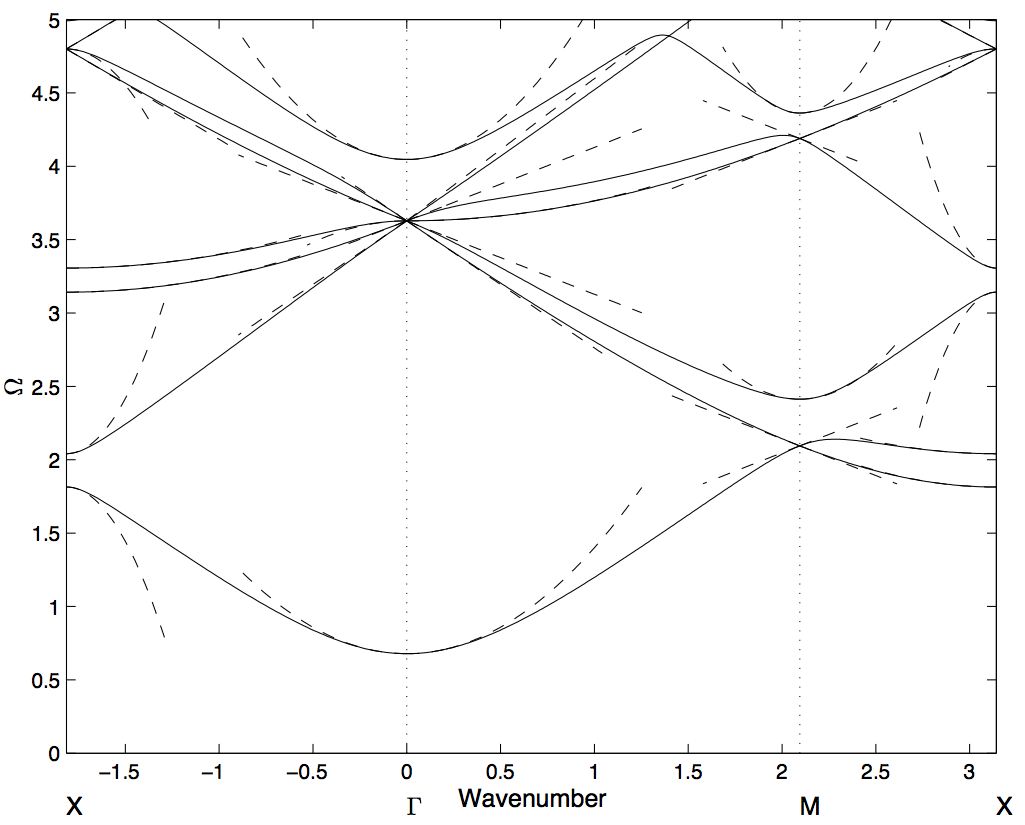
Fig. 3: Band diagram for the hexagonal lattice of Dirichlet points in the Helmholtz case. Solid lines are from equation (52), with the HFH asymptotics shown as dashed curves.

A recurrent feature in literature is that of star-shaped, highly directional wave propagation at specific frequencies, which has emerged in experiments and theory in optics [11, 14], and is perhaps most strikingly seen in mass-spring lattice systems [6, 30, 14], as well as in frame structures [13, 12]. HFH can be used to interpret these effects through the tensor coefficient $T_{ij}$, and we demonstrate this for both the the Helmholtz and the Kirchhoff-Love equation.

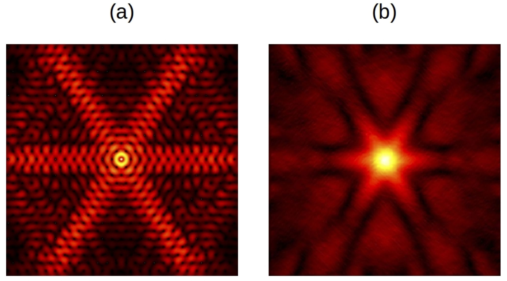
Fig. 4: The Helmholtz case: A star shape is obtained by exciting the center of a hexagonal array of clamped points at frequency $\Omega=1.85$, near the first mode at point $X$ in fig. 3. Panel (a) is the full finite element simulation, where the source is approximated by a narrow Gaussian, and panel (b) is the HFH counterpart, also computed with finite elements, obtained by adding the field at point $X$ to its $\pm 2\pi/3$ rotations. In both cases, PML is used to avoid reflections at the boundary of the domain.

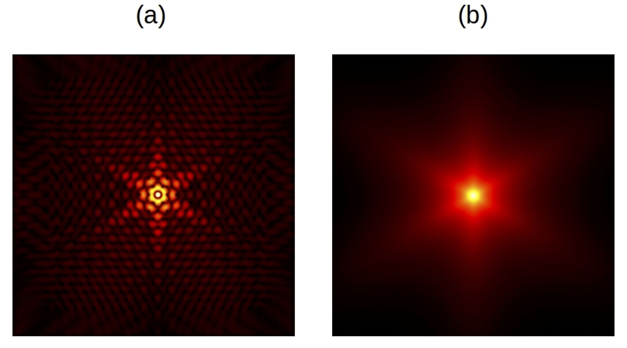
Fig. 5: The Helmholtz case: A star shape is obtained by exciting the center of a hexagonal array of clamped points at frequency $\Omega=2.041$, near the second mode at point $X$ in fig. 3. Panel (a) is the full finite element simulation, where the source is approximated by a narrow Gaussian, and panel (b) is the HFH counterpart, also computed with finite elements, obtained by adding the field at point $X$ to its $\pm 2\pi/3$ rotations. In both cases, PML is used to avoid reflections at the boundary of the domain.

The dynamic anisotropy seen in figs. 4 and 5 is qualitatively explained by the curvature of the dispersion curves near point $X$ in Fig. 3. Near the first band for $\Omega\sim 1.85$ we have $T_{11}T_{22}<0$ (see table 2), signifying an effective PDE that is hyperbolic, not elliptic. The star shape is formed by waves that are directed along the characteristics of this PDE. The angle between the characteristics is twice the inverse tangent of the ratio $\sqrt{|T_{11}/T_{22}|}$. The effect in fig. 5 appears similar but is fundamentally different. Both $T_{ii}$ coefficients are positive but $T_{22}/T_{11}\gg 1$. The propagation is thus directed along the $\mathbf{j}$-direction, and the sum of this with its $2\pi/3$ symmetry rotations yield the effect. This is identical to the effect seen for the analogous discrete system [33].

$T_{11}$	$T_{22}$	$\Omega_{0}$
$1$	$-13.6253$	$1.8141$
$0.8262$	$15.5661$	$2.0409$

Table 2: The first two standing wave frequencies for a hexagonal cell with clamped holes at wavenumber ${\boldsymbol{\kappa}}=(0,\pi/\sqrt{3})$ at $X$, The above coefficients are used in Fig. 3

5.1.2 Honeycomb array

The honeycomb array can be obtained from the hexagonal lattice by including two inclusions in each unit cell (fig. 6), located at points given by

(67) $${\bf I}^{(1,2)}=\pm\frac{1}{2\sqrt{3}}\left(\sqrt{3}{\bf i}+{\bf j}\right),$$

where $\pm$ correspond to the first and second inclusions respectively. Using equation (52) we find the dispersion relation from the zeros of the determinant,

(68) $$\varrho_{1,1}\pm|\varrho_{1,2}|=0,$$

where the reciprocal lattice vector is

(69) $${\bf G}=\pi\left[n,\frac{1}{\sqrt{3}}\left(2m-n\right)\right].$$

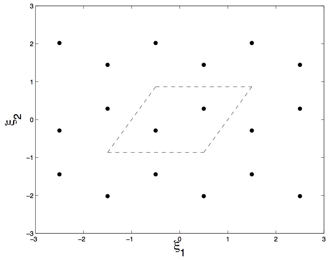
Fig. 6: The honeycomb arrangement of inclusions with the elementary cell, containing two inclusions, shown by the dashed lines.

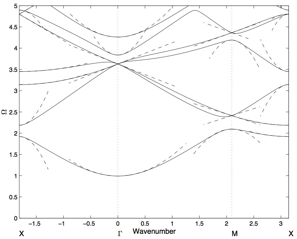
Fig. 7: The band diagram for a honeycomb arrangement of Dirichlet inclusions in the Helmholtz case. Solid lines from equation (68) and the dashed lines are from the HFH asymptotics.

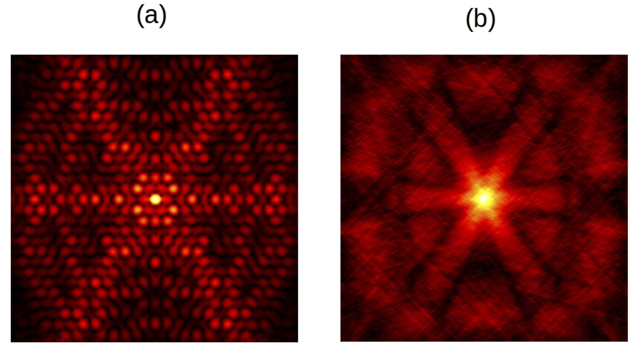
Fig. 8: The Helmholtz case: A star shape is obtained by exciting the center of a honeycomb array of Dirichlet points at frequency $\Omega=1.938$, near the first mode at point $X$ in fig. 7. Panel (a) is the full finite element simulation, where the source is approximated by a narrow Gaussian, and panel (b) is the HFH counterpart, also computed with finite elements, obtained by adding the field at point $X$ to its $\pm 2\pi/3$ rotations. In both cases, PML is used to avoid reflections at the boundary of the domain.

The dispersion diagram for the honeycomb array, shown in Fig. 7, shares several features with that of the hexagonal array (Fig. 3). It too exhibits a generalised Dirac point at $\Gamma$, but in this case with one fewer branch, and also contains saddle points that yield hyperbolic behaviour and the characteristic star shapes. An additional feature here is the small omni-directional band gap for $2.09<\Omega<2.19$, which has implications for the existence of localised defect modes in the honeycomb structure. Localised defect states were analysed in detail for the discrete analogue of HFH in [32], and here we consider the effect of introducing a finite defect by means of removing one or more pins from the honeycomb array. If the size and shape of the defect is appropriately chosen, and the perturbed array treated in the context of an eigenvalue problem, we observe a localised state, in which the field decays evanescently in the surrounding medium. The decay rate of the envelope function is then governed by equation (26). Our effective medium approach may be applied inside any stop-band, and here we demonstrate this both for the zero-frequency gap (fig. 9) and also inside the narrow gap $2.09<\Omega<2.19$ (fig. 10). There is currently much interest in such localised modes, for example in the context of opto-mechanical problems [23], where the simultaneous localisation of electromagnetic and elastic modes has applications for, among other things, optical cooling. Analysis of localised defect states is also fundamental to the field of photonic crystal fibres [43].

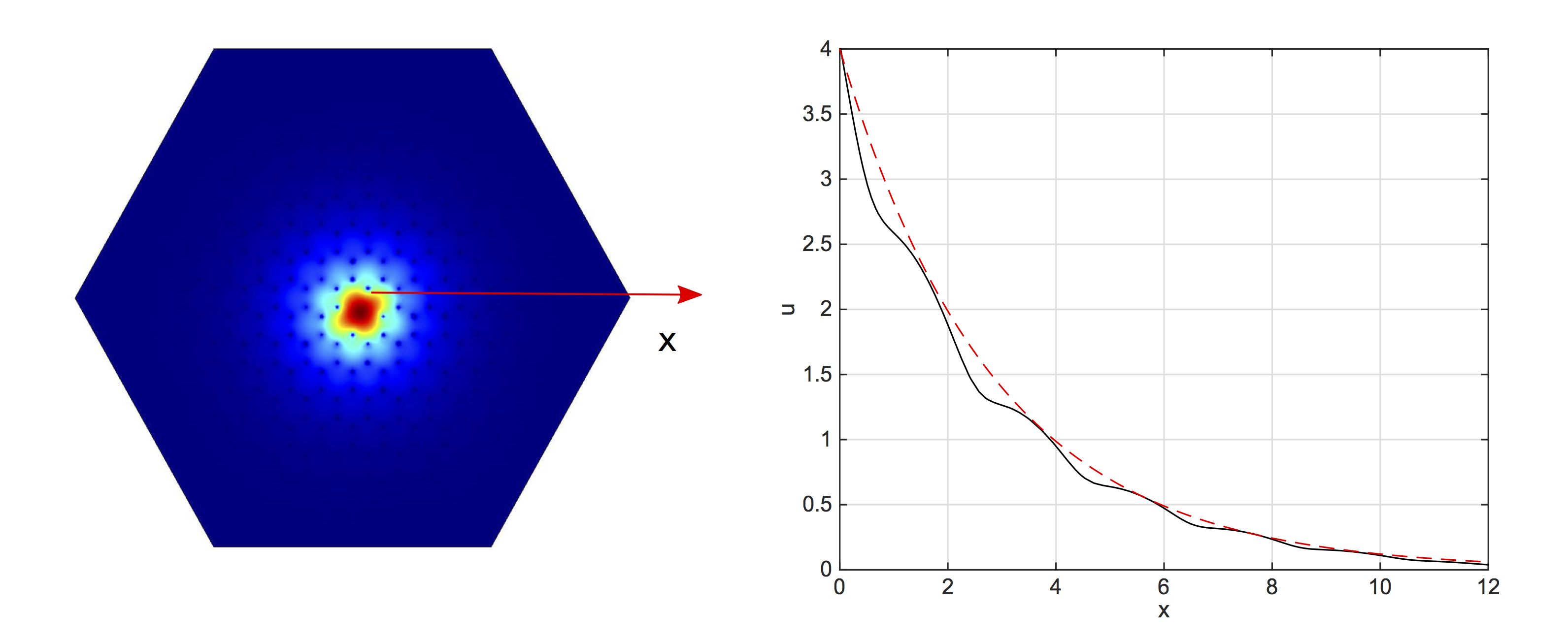
Fig. 9: The Helmholtz case: Localised defect mode at $\Omega=0.93$, induced by the removal of two adjacent pins, which lies in the zero-frequency stop-band just beneath the lowest eigenvalue at $\Gamma$. The effective equation is $0.97f_{0,xx}+0.97f_{0,yy}+(\Omega^{2}-\Omega_{0}^{2})f_{0}=0$, where $\Omega_{0}=0.992$, which leads to an isotropically decaying envelope (the red dashed curve).

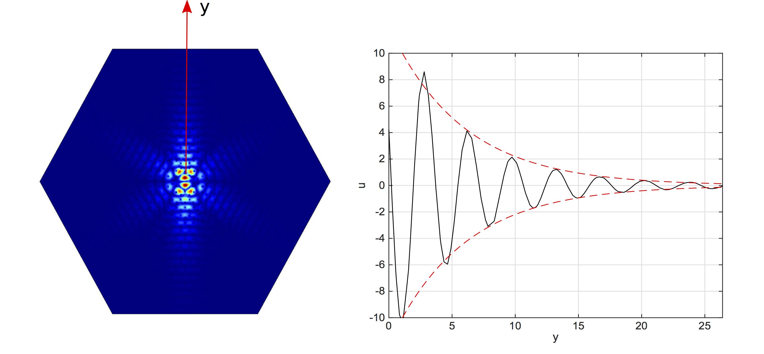
Fig. 10: The Helmholtz case: Localised defect mode at $\Omega=2.16$, induced by removing six adjacent pins, which lies in the narrow stop-band $2.09<\Omega<2.19$. The dominant effective equation is $0.95f_{0,xx}+12.41f_{0,yy}+(\Omega^{2}-\Omega_{0}^{2})f_{0}=0$, where $\Omega_{0}=2.187$, corresponding to the second lowest eigenvalue at $X$, which leads to highly directed leakage in the vertical direction, and hence in 6 directions by rotational symmetry of the array. Note that this is one of two independent defect modes at this frequency, and the directivity can be primarily along any one of the 6 symmetric directions, corresponding to different linear combinations of these two.

5.1.3 Rhombic lattice

The final lattice we consider is the least symmetric of our examples, and the resulting irreducible Brillouin zone has four vertices, rather that three. Fig. 11 shows the dispersion diagram for the rhombic lattice, and demonstrates how HFH captures the group velocity and curvature at any point in the Brillouin zone. As the discretisation of the Brillouin zone becomes more dense, the exact dispersion curves can be retrieved via the asymptotic method. As an aside, an interesting nuance is observed whereby the dispersion curves are symmetric about $Q$ along the path $NM$. Further investigation reveals that this symmetry is only present along that particular path, as is clear from the isofrequency plot Fig. 13. The dispersion curves near points $N$ and $M$ are linear as it is shown by Fig. 12, despite appearing to have locally quadratic behaviour. The group velocity is non-zero at these points, even though the dispersion surface admits local extrema.

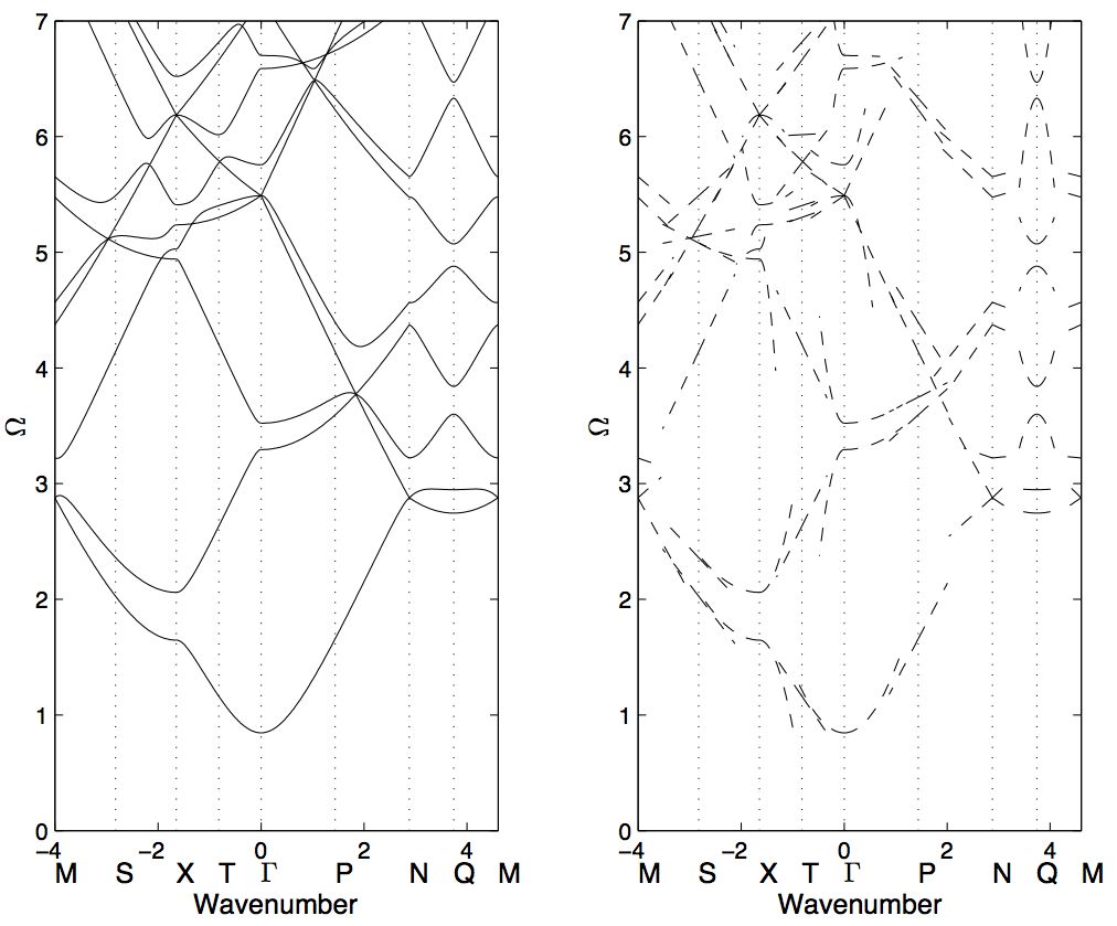
Fig. 11: The band diagram for the rhombic lattice in the Helmholtz case: Left panel showing with solid lines the exact dispersion relation for the rhombic lattice ($\alpha=0.7$). Asymptotics are shown in the right panel as dashed lines and found by perturbing away from the corners of the Brillouin zone, $\Gamma$, $N$, $M$ and $X$ as well as the mid-points of $\Gamma N$, $NM$, $MX$, $M\Gamma$, namely $P$, $Q$, $S$, $T$ respectively.

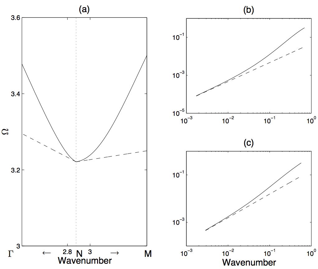
Fig. 12: Close-up plot of third branch of the band diagram of fig. 11 with asymptotics (dashed) as well as loglog plots. Panel (a) shows the close-up of the third branch near point $N$ of the Brillouin zone. In panel (a) the power law of the dispersion curve is unclear but panels (b) and (c) show that the latter is linear and the asymptotics by HFH match well the dispersion curves.

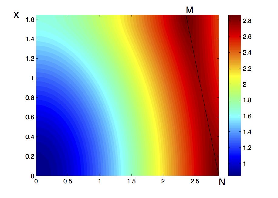
Fig. 13: Isofrequency curve for first mode of rhombus geometry which demonstrates symmetry along the NM path

5.2 Kirchhoff-Love equation

5.2.1 Hexagonal lattice

In the case of the Kirchhoff-Love model, we opt to solely examine inclusions arranged in a hexagonal lattice. Similar features dispersive features are observed, An interesting distinction between the curves for the Helmholtz equation and those of Kirchhoff-Love, is that the latter model is far more sensitive to changes in the radii of the inclusions. This can be seen in the dispersion curves (fig. 14), where the solid curves are for finite (but very small) radius inclusions ($R=0.01$) and the dashed curves are for zero-radius holes, found using the exact solution, equation (52). This nuance can be explained by comparing the two dispersion curves, (figures 3 and 14) and noting that the frequencies in the plate model are considerably higher than those found using Helmholtz equation. Hence as the frequency increases the dashed lines deviate further from the solid lines.

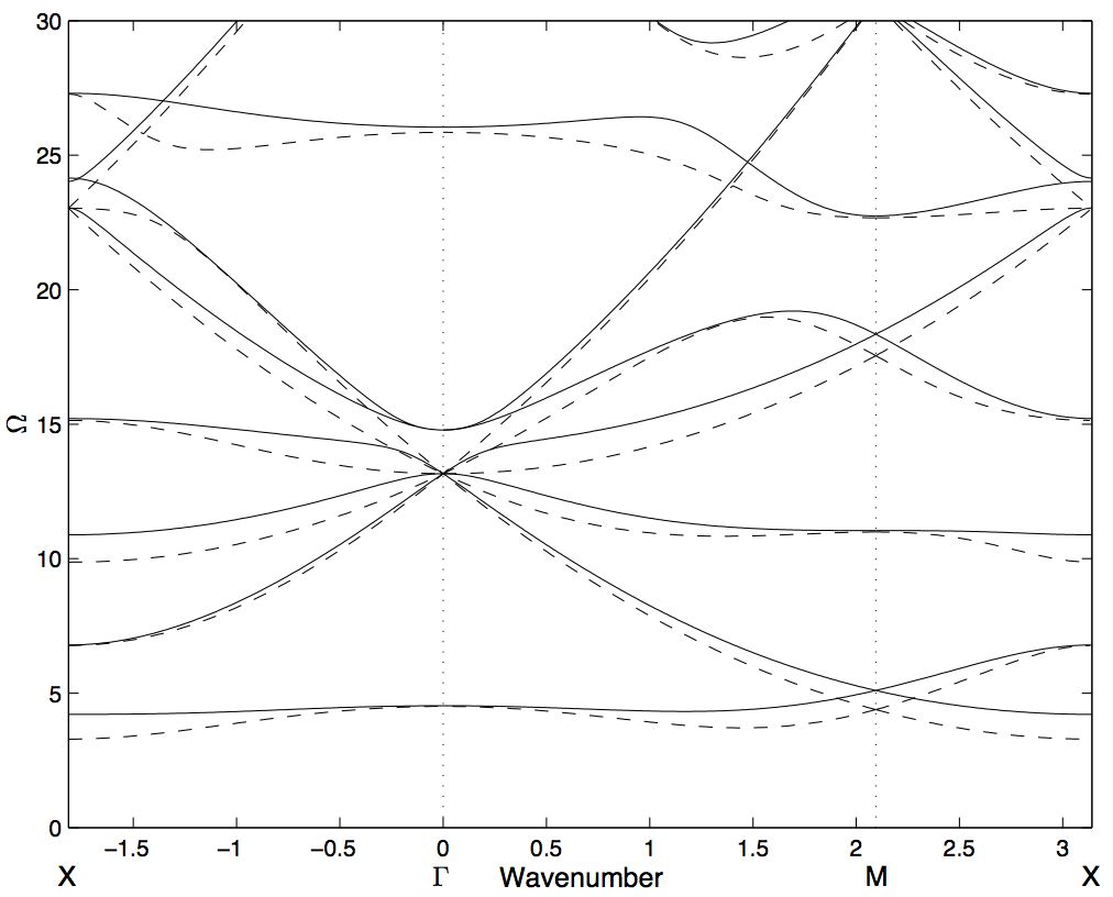
Fig. 14: Dispersion curves for the Kirchhoff-Love model with inclusions arranged in a hexagonal lattice. Solid curves are for finite radius inclusions ($R=0.01$) whilst the dashed lines are for the pinned points, equation (63).

$T_{11}$	$T_{22}$	$\Omega_{0}$	Radius
$37.9829$	$-35.8258$	$6.7903$	$0.01$
$71.3788$	$-29.1596$	$6.7733$	Pinned

Table 3: The $T_{ij}$ coefficients found in equation (42) and frequency values for both the finite radius holes and for the pinned points are shown for the second mode at point X in the dispersion curve (fig. 14). The values for the pinned points are taken from equation (66). Note the strong mismatch between the $T_{ij}$ coefficients for small clamped inclusions and pinned points.

The strong discrepancies between a small change in radius is demonstrated in table 3 for the second mode at point X in fig. 14. This mode is of interest, as excitation about this frequency yields star shape oscillations (fig. 15) similar to those seen earlier for the Helmholtz equation. This oscillatory pattern can be equivalently ascertained by taking into account the inherent three-fold symmetry of our medium and the hyperbolic PDE obtained using HFH.

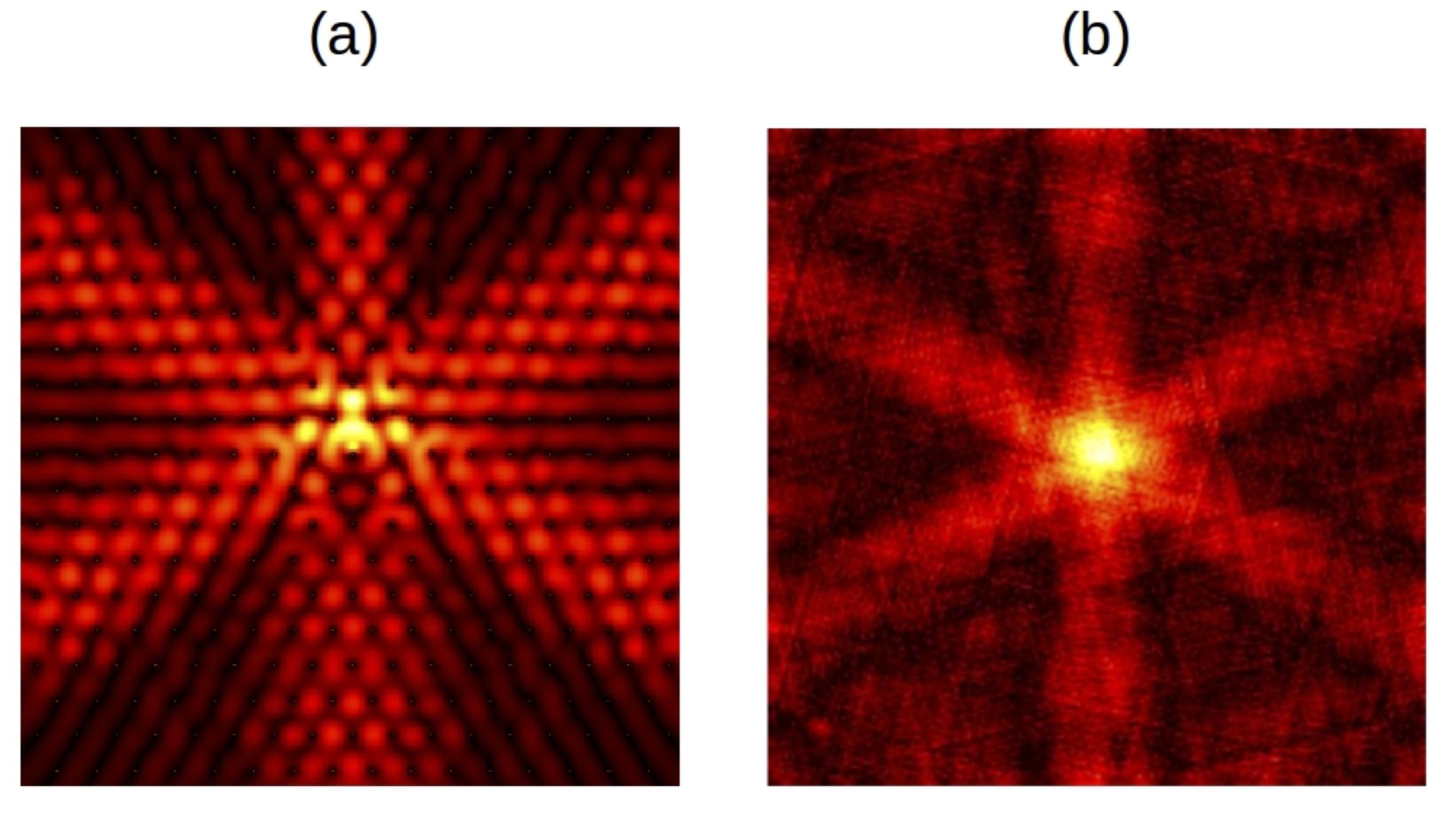
Fig. 15: A star shape is obtained by exciting the center of a hexagon array of clamped points at frequency $\Omega=6.7903$ for the Kirchhoff-Love model, near the second mode at point X in figure 14. Panel (a) shows the plate simulation, whilst panel (b) is the HFH effective medium simulation, both are for the finite radius of $R=0.01$. Similar to the Helmholtz case the three characteristics are obtained due to the inherent three-fold symmetry of the structure.

6 Concluding remarks

It is clear that a microstructured medium with any periodic arrangement of inclusions can now be homogenised for any frequency in the Bloch spectrum and effective continuum equations deduced. In contrast to the previously studied case of orthogonal lattices [3], a key technical difficulty is that the microscale and macroscale are naturally in different coordinate systems. Once this issue has been overcome the effective equations are versatile and capture, for instance, the strongly directional anisotropic behaviour at critical frequencies. The validity and usefulness of our homogenisation method is demonstrated with the topical honeycomb arrangement of inclusions, whereby we introduce defects on the microscale and show that the envelope modulation in the surrounding medium is perfectly captured by our long-scale effective PDE. Additionally, due to the mathematical similarity between Helmholtz and Kirchhoff-Love equations, we apply our analysis to both of these models, and find that the former helps us to better understand the latter. Finally, exact solutions are constructed for constrained points using Fourier series and these are used to provide analytical expressions within our asymptotic framework.

References

• [1] G. Allaire and A. Piatnitski, Homogenisation of the Schrödinger equation and effective mass theorems, Commun. Math. Phys., 258 (2005), pp. 1–22.
• [2] T. Antonakakis and R. V. Craster, High frequency asymptotics for microstructured thin elastic plates and platonics, Proc. R. Soc. Lond. A, 468 (2012), pp. 1408–1427.
• [3] T. Antonakakis, R. V. Craster, and S. Guenneau, High-frequency homogenization of zero frequency stop band photonic and phononic crystals, New J. Phys, 15 (2013), p. 103014.
• [4]  , Homogenization for elastic photonic crystals and metamaterials, J. Mech. Phys. Solids, 71 (2014), pp. 84–96.
• [5] T. Antonakakis, R. V. Craster, and S. Guenneau, Moulding and shielding flexural waves in elastic plates, Euro. Phys. Lett., 105 (2014), p. 54004.
• [6] M. V. Ayzenberg-Stepanenko and L. I. Slepyan, Resonant-frequency primitive waveforms and star waves in lattices, J. Sound Vib., 313 (2008), pp. 812–821.
• [7] M. S. Birman and T. A. Suslina, Homogenization of a multidimensional periodic elliptic operator in a neighborhood of the edge of an internal gap, Journal of Mathematical Sciences, 136 (2006), pp. 3682–3690.
• [8] C. Boutin, A. Rallu, and S. Hans, Large scale modulation of high frequency waves in periodic elastic composites, J. Mech. Phys. Solids, 70 (2014), pp. 362–381.
• [9] L. Brillouin, Wave propagation in periodic structures: electric filters and crystal lattices, Dover, New York, second ed., 1953.
• [10] S. Brule, E. Javelaud, S. Enoch, and S. Guenneau, Experiments on seismic metamaterials moulding surface waves, Phys. Rev. Lett., 112 (2014).
• [11] D. N. Chigrin, S. Enoch, C. M. S. Torres, and G. Tayeb, Self-guiding in two-dimensional photonic crystals, Optics Express, 11 (2003), pp. 1203–1211.
• [12] D. J. Colquitt, R. V. Craster, and M. Makwana, High frequency homogenisation for elastic lattices, Quart. Jl. Mech. Appl. Math., (2015). in press.
• [13] D. J. Colquitt, I. S. Jones, N. V. Movchan, A. B. Movchan, and R. C. McPhedran, Dynamic anisotropy and localization in elastic lattice systems, Waves in Random and Complex Media, 22 (2012), pp. 143–159.
• [14] R. V. Craster, T. Antonakakis, M. Makwana, and S. Guenneau, Dangers of using the edges of the Brillouin zone, Physical Review B, 86 (2012).
• [15] R. V. Craster and S. Guenneau, eds., Acoustic Metamaterials, Springer-Verlag, 2012.
• [16] R. V. Craster, L. M. Joseph, and J. Kaplunov, Long-wave asymptotic theories: The connection between functionally graded waveguides and periodic media, Wave Motion, 51 (2014), pp. 581–588.
• [17] R. V. Craster, J. Kaplunov, and A. V. Pichugin, High frequency homogenization for periodic media, Proc R Soc Lond A, 466 (2010), pp. 2341–2362.
• [18] M. Dubois, M. Farhat, E.Bossy, S.Enoch, S.Guenneau, and P.Sebbah, Flat lens for pulse focusing of elastic waves in thin plates, Appl. Phys. Lett., 103 (2013).
• [19] D. V. Evans and R. Porter, Penetration of flexural waves through a periodically constrained thin elastic plate floating in vacuo and floating on water, J. Engng. Math., 58 (2007), pp. 317–337.
• [20] M. Farhat, S. Guenneau, and S. Enoch, High-directivity and confinement of flexural waves through ultrarefraction in thin perforated plates, European Physics Letters, 91 (2010), p. 54003.
• [21] M. Farhat, S. Guenneau, S. Enoch, A. Movchan, and G. Petursson, Focussing bending waves via negative refraction in perforated thin plates, Appl. Phys. Lett., 96 (2010), p. 081909.
• [22] C. Fefferman and M. I. Weinstein, Honeycomb lattice potentials and dirac points, J. Amer. Math. Soc, 25 (2012), pp. 1169–1220.
• [23] E. Gavartin, R. Braive, I. Sagnes, O. Arcizet, A. Beveratos, T. J. Kippenberg, and I. Robert-Philip, Optomechanical coupling in a two-dimensional photonic crystal defect cavity, Phys. Rev. Lett., (2011).
• [24] D. Gridin, R. V. Craster, and A. T. I. Adamou, Trapped modes in curved elastic plates, Proc R Soc Lond A, 461 (2005), pp. 1181–1197.
• [25] M. A. Hoefer and M. I. Weinstein, Defect modes and homogenization of periodic Schrödinger operators, SIAM J. Math. Anal., 43 (2011), pp. 971–996.
• [26] J. D. Joannopoulos, S. G. Johnson, J. N. Winn, and R. D. Meade, Photonic Crystals, Molding the Flow of Light, Princeton University Press, Princeton, second ed., 2008.
• [27] J. Kaplunov, Equations for high-frequency long-wave vibrations of an elastic layer lying on an acoustic half-space, Doklady Akad. Nauk SSSR, 309 (1989), pp. 1077–1081.
• [28] J. D. Kaplunov, G. A. Rogerson, and P. E. Tovstik, Localized vibration in elastic structures with slowly varying thickness, Quart. J. Mech. Appl. Math., 58 (2005), pp. 645–664.
• [29] C. Kittel, Introduction to solid state physics, John Wiley & Sons, New York, 7th ed., 1996.
• [30] R. S. Langley, The response of two-dimensional periodic structures to point harmonic forcing, J. Sound Vib., 197 (1997), pp. 447–469.
• [31] B. R. Mace, The vibration of plates on two-dimensionally periodic point supports, J. Sound Vib., 192 (1996), pp. 629–643.
• [32] M. Makwana and R. V. Craster, Localised point defect states in asymptotic models of discrete lattices, Quart. J. Mech. Appl. Math., (2013).
• [33]  , Homogenisation for hexagonal lattices and honeycomb structures, Quart. J. Mech. Appl. Math., (2014).
• [34] R. McPhedran, A. B. Movchan, N. V. Movchan, M. Brun, and M. J. A. Smith, Trapped modes and steered Dirac cones in platonic crystals. arXiv:1410.0393, 2015.
• [35] P. D. Metcalfe, Localization and delocalization on fluid-loaded elastic structures, PhD thesis, DAMTP, University of Cambridge, 2002.
• [36] A. B. Movchan, N. V. Movchan, and R. C. McPhedran, Bloch-Floquet bending waves in perforated thin plates, Proc. R. Soc. Lond. A, 463 (2007), pp. 2505–2518.
• [37] A. H. C. Neto, F. Guinea, N. M. R. Peres, K. S. Novoselov, and A. K. Geim, The electronic properties of graphene, Rev. Modern Phys., (2009), pp. 109–162.
• [38] M. Ruppin, F. Lemoult, G. Lerosey, and P. Roux, Experimental demonstration of ordered and disordered multiresonant metamaterials for lamb waves, Phys. Rev. Lett., 112 (2014).
• [39] M. J. A. Smith, M. H. Meylan, and R. C. McPhedran, Flexural wave filtering and platonic polarisers in thin elastic plates, Q. Jl. Mech. Appl. Math., 66 (2013), pp. 437–463.
• [40] D. Torrent, D. Mayou, and J. Sanchez-Dehesa, Elastic analog of graphene: Dirac cones and edge states for flexural waves in thin plates, Phys. Rev. B, 87 (2013), p. 115143.
• [41] Z. Wu, K. Xie, and H. Yang, Band gap properties of two-dimensional photonic crystals with rhombic lattice, Optik, 123 (2012), pp. 534–536.
• [42] Z. H. Wu, K. Xie, H. J. Yang, P. Jiang, and X. J. He, All-angle self-collimation in two-dimensional rhombic-lattice photonic crystals, J. Opt. A, 14 (2012), p. 015002.
• [43] F. Zolla, G. Renversez, A. Nicolet, B. Kuhlmey, S. Guenneau, and D. Felbacq, Foundations of photonic crystal fibres, Imperial College Press, London, 2005.