Modeling county level breast cancer survival data using a covariate-adjusted frailty proportional hazards model

Abstract

Understanding the factors that explain differences in survival times is an important issue for establishing policies to improve national health systems. Motivated by breast cancer data arising from the Surveillance Epidemiology and End Results program, we propose a covariate-adjusted proportional hazards frailty model for the analysis of clustered right-censored data. Rather than incorporating exchangeable frailties in the linear predictor of commonly-used survival models, we allow the frailty distribution to flexibly change with both continuous and categorical cluster-level covariates and model them using a dependent Bayesian nonparametric model. The resulting process is flexible and easy to fit using an existing R package. The application of the model to our motivating example showed that, contrary to intuition, those diagnosed during a period of time in the 1990s in more rural and less affluent Iowan counties survived breast cancer better. Additional analyses showed the opposite trend for earlier time windows. We conjecture that this anomaly has to be due to increased hormone replacement therapy treatments prescribed to more urban and affluent subpopulations.

FLA

, ,
and T1Supported by NCI Grants R03CA165110 and 5R03CA176739, and ASPIRE grant from the University of South Carolina. T2Supported by Fondecyt Grant 1141193.

1 Introduction

Based on data gathered for Iowa State in the Surveillance Epidemiology and End Results (SEER) program of the National Cancer Institute, we assess the effect of potential risk factors for womens’ breast cancer. This involves the analysis of clustered time-to-event right-censored data, where event times of patients from the same county of residence are expected to be associated with each other, possibly due to sharing common unobserved characteristics, such as region-specific differences in environments, treatment resources or diagnosis of the patients. As is widely known, taking into account the clustered nature of the data is a must to obtain valid statistical inferences [see, e.g., Therneau and Grambsch (2000), Chapter 8].

A standard way of modeling clustered survival data is to introduce a common random effect (frailty) into the survival model for each cluster, yielding shared frailty models. “Frailties,” termed by Vaupel, Manton and Stallard (1979), were originally introduced to deal with possible heterogeneity due to unobserved covariates and are regarded as unobserved common characteristics for each cluster able to account for the dependence among event times. In the context of the proportional hazards (PH) model, as conventionally implemented, frailties are incorporated into the linear predictor, and the median or mean of the frailty distribution is constrained to be zero to avoid identifiability problems. Conditional on the frailty, the model retains its interpretation in terms of constants of proportionality of the hazards. Survival models with frailties have been extensively used in the statistical literature, especially when the comparison of event times within cluster is of interest.

A common assumption in shared frailty survival models is the one of homogeneity, where the frailties are assumed to be independent and identically distributed (i.i.d.) random variables from a parametric or nonparametric distribution [see, e.g., Clayton and Cuzick (1985), Gustafson (1997), Qiou, Ravishanker and Dey (1999), Walker and Mallick (1997)]. Although the nonparametric approach provides flexibility in capturing a frailty distribution’s variance, skewness, shape and even modality, it essentially assumes that these frailty distributional aspects are the same across all the clusters, which may be restrictive for particular data sets [Noh, Ha and Lee (2006)]. For example, in the kidney transplantation study, Liu, Kalbfleisch and Schaubel (2011) argue that the frailty distribution may be affected by some cluster-level covariates, since “…urban transplant facilities may exhibit more uniform practices than rural transplant hospitals, corresponding to less heterogeneity (smaller variance) for frailties of urban centers…” Ignoring such heterogeneity can drastically affect the inference for cluster-specific effects and prediction [McCulloch and Neuhaus (2011)].

As the process generating the frailty terms is on its own right of scientific interest, different extensions of the i.i.d. frailty modeling approach have been considered. Wassell and Moeschberger (1993) studied the impact of interventions in the Framingham Heart Study by introducing a modified gamma frailty with a pairwise covariate-dependent parameter. Yashin and Iachine (1999) considered the dependence between frailty and observed covariates (BMI and smoking) in Danish twins to investigate the heritability of susceptibility to death. Noh, Ha and Lee (2006) verified frailty distribution heterogeneity in a well-known kidney infection data set by applying a dispersed normal model. Cottone (2008) assumed either Bernoulli or normal distributions for the frailties where the frailty distribution mean or variance depends on cluster-level covariates through specified link functions. Liu, Kalbfleisch and Schaubel (2011) proposed a covariate-dependent positive stable shared frailty model with an application to kidney transplantation data from the Scientific Registry of Transplant Recipients, and demonstrated the heterogeneity in facility performance. Wang and Louis (2004) studied a related approach for binary data that has both conditional and marginal interpretation using the so-called bridge distribution instead of positive stable.

The previously described model extensions allow for particular and specific aspects of distributional shape to change with cluster-level covariates. However, a more thorough evaluation of the effect of the predictors should account for potential changes in characteristics of the frailty distribution other than just, for example, the location or scale. It is, for instance, useful to examine potential changes in the skewness, symmetry and multimodality of the frailty distribution. Therefore, a nonparametric formulation that anticipates changes in shape, skew and modality beyond simple location models is of interest.

In this paper, we propose a practicable and general framework for modeling clustered survival data as a function of covariates, based on a predictor-dependent Bayesian nonparametric model for the frailties and the Cox’s PH model. Under the proposed approach the frailty distribution flexibly changes with both continuous and categorical cluster-level covariates, thus allowing for full heterogeneity across clusters. We apply this modeling approach to a subset of the SEER county-level breast cancer data consisting of 1073 women diagnosed with malignant breast cancer during 1995–1998. Important patient-level covariates include age at diagnosis, race, county of residence and the stage of the disease. Additional county-level covariates potentially associated with breast cancer survival are also available from census data, including median household income, poverty level, education and a rurality measure. These area-level socioeconomic factors have been discovered to be associated with breast cancer by many researchers [e.g., Sprague et al. (2011)]. Women living in more affluent or less rural geographic areas tend to survive breast cancer better after a diagnosis than those living in regions with indicators of low socioeconomic status. Moreover, rural counties may present more heterogeneity in access to quality care and screening for breast cancer, leading to more variability for frailties of rural counties [Zhao and Hanson (2011)]. This suggests to us that the frailty distribution could be potentially affected by these county-level socioeconomic factors. The results show that the proposed model provides better goodness of fit to the data and is predictively superior to the traditional PH spatial frailty model, as well as helping to piece together a plausible story for the data in terms of the prescribing of hormone replacement therapy.

The paper is organized as follows. In Section 2 we introduce the proposed frailty PH model, including a detailed description of the dependent Bayesian nonparametric model and the Markov chain Monte Carlo (MCMC) implementation of the posterior computations. Section 3 provides a detailed analysis of the motivating data set. Section 4 presents the results of simulation studies to evaluate the performance of the proposed model. Some concluding remarks and a final discussion are given in Section 5.

2 Covariate-adjusted frailty proportional hazards model

2.1 The modeling approach

Suppose that right-censored survival data $(\mathbf{w}_{ij},t_{ij},\delta_{ij})$ are collected for the $j$th subject of the $i$th cluster, where $j=1,\ldots,n_{i}$, $i=1,\ldots,n$, $\mathbf{w}_{ij}$ is a $p$-dimensional vector of exogenous covariates, $t_{ij}$ is the recorded event time, and $\delta_{ij}$ is the censoring indicator equaling $1$ if $t_{ij}$ is an observed event time and equaling $0$ if the event time is right-censored at $t_{ij}$. Let $T_{ij}$ and $C_{ij}$ be the event and censoring times, respectively, for the $j$th subject in the $i$th cluster. To take into account the within-cluster association structure, a frailty PH model is assumed for $T_{ij}$. The conditional PH assumption implies that the hazard function of $T_{ij}$ is given by

$$\lambda(t|\mathbf{w}_{ij},e_{i})=\lambda_{0}(t)\exp\bigl{(}\mathbf{w}^{\prime}_{ij}\bolds{\xi}+e_{i}\bigr{)},$$ (1)

where $\mathbf{e}=(e_{1},\ldots,e_{n})^{\prime}$ is an unobserved vector of frailties, and $\lambda_{0}(t)$ is the baseline hazard function corresponding to the event time of a subject with covariates $\mathbf{w}=\mathbf{0}$ and $e=0$. We additionally assume a conditionally independent censoring scheme, that is, $C_{ij}$ and $T_{ij}$ are independent given $\mathbf{w}_{ij}$ and $e_{i}$. Often the frailties are assumed to be exchangeable or i.i.d. from some parametric or nonparametric distribution $G$. For instance, Therneau, Grambsch and Pankratz (2003) considered exchangeable Gaussian frailties and proposed an estimation procedure based on a Laplace approximation of the likelihood function leading to a penalized partial likelihood. This approach, referred to below as GF, will be compared with our method in the simulation studies.

Now consider a partition of the predictor vector $\mathbf{w}_{ij}=(\tilde{\mathbf{w}}^{\prime}_{ij},\mathbf{x}^{\prime}_{i})^{\prime}$, where $\mathbf{x}_{i}\in\mathcal{X}\subseteq\mathbf{R}^{q}$ is a $q$-dimensional vector of cluster-level covariates and $\tilde{\mathbf{w}}_{ij}$ is a $(p-q)$-dimensional vector of subject-specific covariates, respectively, and the corresponding partition of the regression coefficient vector $\bolds{\xi}=(\tilde{\bolds{\xi}}{}^{\prime},\bolds{\xi}^{\prime}_{x})^{\prime}$. On the scale of the linear predictor $\mathbf{w}^{\prime}_{ij}\bolds{\xi}+e_{i}$, the frailty $e_{i}$ models the cluster-specific behavior and its distribution $G$ is shifted by $\mathbf{x}^{\prime}_{i}\bolds{\xi}_{x}$. Therefore, the homogeneity assumption implies that the vector of cluster-level covariates $\mathbf{x}_{i}$ modifies only the location of the distribution of cluster-specific effects but not its shape. To relax this assumption, we consider a covariate-adjusted frailty PH model, where the frailty distribution depends on cluster-level covariates $\mathbf{x}_{i}$. That is,

$$e_{i}|G_{\mathbf{x}_{i}}\stackrel{{\scriptstyle\mathrm{ind}.}}{{\sim}}G_{\mathbf{x}_{i}},$$

where for every $\mathbf{x}\in\mathcal{X}$, $G_{\mathbf{x}}$ is a probability measure defined on $\mathbb{R}$; this specifies a probability model for the entire collection of probability measures $\mathcal{G}^{\mathcal{X}}=\{G_{\mathbf{x}}\dvtx\mathbf{x}\in\mathcal{X}\}$, such that its elements are allowed to smoothly vary with the cluster-level covariates $\mathbf{x}$. Specifically, we consider a mixture of linear dependent tailfree processes (LDTFP) prior [Jara and Hanson (2011)] for $\mathcal{G}^{\mathcal{X}}$, denoted as

$$\mathcal{G}^{\mathcal{X}}|J,h,\theta,c,\rho\sim\operatorname{LDTFP}\bigl{(}h,\Pi^{J,\theta},\mathcal{A}^{J,c,\rho}\bigr{)},$$

and

$$c|Q\sim Q,$$

where $J\in\mathbb{N}$ is the level of specification of the process, $c\in\mathbb{R}_{+}$ is a prior precision parameter controlling the prior variability of the process, $h(\cdot)=\frac{\exp\{\cdot\}}{1+\exp\{\cdot\}}$, $\Pi^{J,\theta}$ is a $J$-level sequence of binary partitions of $\mathbb{R}$, depending on the scale parameter $\theta\in\mathbb{R}_{+}$, $\mathcal{A}^{J,c,\rho}=\{2n/c\rho(1),\ldots,2n/c\rho(J)\}$ is a collection of positive numbers depending on $J$, $c$ and $\rho$, $\rho\dvtx\mathbb{N}\longrightarrow\mathbb{R}_{+}$ is an increasing function, and $Q$ is a probability measure defined on $\mathbb{R}_{+}$.

The LDTFP is specified such that for every $\mathbf{x}\in\mathcal{X}$, the process $G_{\mathbf{x}}$ is centered around an $N(0,\theta)$ distribution, that is, $E(G_{\mathbf{x}})=N(0,\theta)$, for every $\mathbf{x}\in\mathcal{X}$. Furthermore, the process is specified such that for every $\mathbf{x}\in\mathcal{X}$, $G_{\mathbf{x}}$ is almost surely a median-zero probability measure. The latter property is important to avoid identifiability problems. The LDTFP process includes as important special cases a nonparametric exchangeable frailty model where $G_{\mathbf{x}}=G_{\mathbf{x}^{\prime}}$ for $\mathbf{x}^{\prime}\neq\mathbf{x}$ as well as exchangeable normal frailties $G_{\mathbf{x}}=N(0,\theta)$ for all $\mathbf{x}\in\mathcal{X}$.

As shown by Jara and Hanson (2011), dependent tailfree processes have appealing theoretical properties, such as continuity as a function of the predictors, large support on the space of conditional density functions, straightforward posterior computation relying on algorithms for fitting generalized linear models, and the process closely matches conventional Polya tree priors [see, e.g., Hanson (2006a)] at each value of the predictor, which justify its choice here. Polya trees have been extensively studied in the literature and have desirable properties in terms of support and posterior consistency. Details on the trajectories of $\operatorname{LDTFP}(h,\Pi^{J,\theta},\mathcal{A}^{J,c,\rho})$, useful for a complete implementation of algorithms for exploring the corresponding posterior distributions, are given in Appendix A of the supplementary material [Zhou et al. (2015)].

Other dependent processes could be considered for $\mathcal{G}^{\mathcal{X}}$, but a highly limiting requirement is that some aspect of the location, for example, mean or median, can be fixed. There are few examples where the process changes smoothly with covariates; one is the multivariate beta process of Trippa, Müller and Johnson (2011). Another approach using Dirichlet process mixtures can be found in Reich, Bondell and Wang (2010), but this latter approach would have to be extended to allow the means or variances of the two mixture components to change with covariates.

2.2 Posterior computation

The conditional likelihood for $(\bolds{\xi},\lambda_{0},\mathbf{e})$ is given by

$$\mathcal{L}(\bolds{\xi},\lambda_{0},\mathbf{e})=\prod_{i=1}^{n}\prod_{j=1}^{n_{i}}\bigl{[}\lambda_{0}(t_{ij})\exp\bigl{(}\mathbf{w}_{ij}^{\prime}\bolds{\xi}+e_{i}\bigr{)}\bigr{]}^{\delta_{ij}}\exp\bigl{\{}-\Lambda_{0}(t_{ij})\exp\bigl{(}\mathbf{w}_{ij}^{\prime}\bolds{\xi}+e_{i}\bigr{)}\bigr{\}},$$

where $\Lambda_{0}(t)=\int_{0}^{t}\lambda_{0}(s)\,ds$ is the cumulative hazard function. The piecewise exponential model provides a flexible framework to deal with the baseline hazard [see, e.g., Walker and Mallick (1997)]. We partition the time period $\mathbb{R}_{+}$ into $K$ prespecified intervals, say, $I_{k}=(a_{k-1},a_{k}],k=1,\ldots,K$, where $a_{0}=0$ and $a_{K}=\max\{t_{ij}\}$. The baseline hazard is assumed to be constant within each interval, that is,

$$\lambda_{0}(t)=\sum_{k=1}^{K}\lambda_{k}I\{t\in I_{k}\},$$

where $\lambda_{1},\ldots,\lambda_{K}$ are unknown hazard values and $I\{A\}$ is the usual indicator function, that is, $1$ when $A$ is true, $0$ otherwise. The prior hazard is specified by the hazard values $\{\lambda_{k}\}_{k=1}^{K}$ and cut-point vector $\mathbf{a}=(a_{1},\ldots,a_{K})$. If the prior on the $\lambda_{k}$’s is taken to be independent gamma distributions and $\{I_{k}\}_{k=1}^{K}$ is a reasonably fine mesh, the gamma process [Kalbfleisch (1978)] is approximated. To determine the cut-point vector $\mathbf{a}$, one can set $a_{k}$ to be the $\frac{k}{K}$th quantile of the empirical distribution of the $t_{ij}$’s, or choose them based on other considerations (see Section 3.2). Some authors have considered random cut-points [see, e.g., Sahu and Dey (2004)]. Regardless, the resulting model implies a Poisson likelihood [Laird and Olivier (1981)] as follows. Let $K(t)=\min\{k\dvtx a_{k}\geq t\}$, $\Delta_{k}(t)=\min\{a_{k},t\}-a_{k-1}$, and $y_{ijk}=\delta_{ij}I\{k=K(t_{ij})\}$. Set $\mathbf{z}_{ijk}=(\bolds{\iota}_{k}^{\prime},\mathbf{w}_{ij}^{\prime})^{\prime}$ and $\bolds{\gamma}=(\bolds{\lambda}^{\prime},\bolds{\xi}^{\prime})^{\prime}$, where $\bolds{\iota}_{k}$ is a $K$-dimensional vector of zeros except the $k$th element is $1$ and $\bolds{\lambda}=(\log(\lambda_{1}),\ldots,\log(\lambda_{K}))^{\prime}$. Then the likelihood for $(\bolds{\gamma},\mathbf{e})$ becomes

$$\mathcal{L}(\bolds{\gamma},\mathbf{e}) = \prod_{i=1}^{n}\prod_{j=1}^{n_{i}}\bigl{[}\exp\bigl{\{}\log(\lambda_{K(t_{ij})})+\mathbf{w}_{ij}^{\prime}\xi+e_{i}\bigr{\}}\bigr{]}^{\delta_{ij}}$$

$$\hskip 29.0pt{}\times\Biggl{[}\prod_{k=1}^{K(t_{ij})}e^{-\exp\{\log(\lambda_{k})+\mathbf{w}_{ij}^{\prime}\xi+e_{i}\}\Delta_{k}(t_{ij})}\Biggr{]}$$

$$= \prod_{i=1}^{n}\prod_{j=1}^{n_{i}}\prod_{k=1}^{K(t_{ij})}\bigl{[}\bigl{(}\exp\bigl{\{}\mathbf{z}_{ijk}^{\prime}\bolds{\gamma}+e_{i}\bigr{\}}\bigr{)}^{y_{ijk}}e^{-\exp\{\mathbf{z}_{ijk}^{\prime}\bolds{\gamma}+e_{i}+\log(\Delta_{k}(t_{ij}))\}}\bigr{]}$$

$$\propto \prod_{i=1}^{n}\prod_{j=1}^{n_{i}}\prod_{k=1}^{K(t_{ij})}p(y_{ijk}|\bolds{\gamma},e_{i}),$$

where $\mu_{ijk}=\exp\{\mathbf{z}_{ijk}^{\prime}\bolds{\gamma}+e_{i}+\log(\Delta_{k}(t_{ij}))\}$ and $p(y_{ijk}|\bolds{\gamma},e_{i})$ is the probability mass function for a Poisson distribution with mean $\mu_{ijk}$. For each $i=1,\ldots,n$, let $N_{i}=\sum_{j=1}^{n_{i}}{K(t_{ij})}$, $\mathbf{y}_{i}=(y_{ijk})$ be an $N_{i}\times 1$ vector with subscript $ijk$ in lexicographical order.

Thus, the proposed covariate-adjusted frailty PH model takes the following hierarchical structure:

$$\mathbf{y}_{i}|\bolds{\gamma},e_{i} \stackrel{{\scriptstyle\mathrm{ind}.}}{{\sim}} \prod_{j=1}^{n_{i}}\prod_{k=1}^{K(t_{ij})}p(y_{ijk}|\bolds{\gamma},e_{i}),$$

$$\bolds{\gamma} \sim N_{K+p}(\bolds{\gamma}_{0},\mathbf{S}_{0}),$$

$$e_{i}|G_{\mathbf{x}_{i}} \stackrel{{\scriptstyle\mathrm{ind}.}}{{\sim}} G_{\mathbf{x}_{i}},$$

$$\mathcal{G}^{\mathcal{X}}|J,h,\theta,c,\rho \sim \operatorname{LDTFP}\bigl{(}h,\Pi^{J,\theta},\mathcal{A}^{J,c,\rho}\bigr{)},$$

$$\theta^{-2} \sim \Gamma(\tau_{1},\tau_{2}),\qquad c\sim\Gamma(a_{c},b_{c}),$$

which largely simplifies computations, where $N_{p}(\mathbf{m},\mathbf{S})$ refers to a $p$-variate normal distribution with mean $\mathbf{m}$ and covariance matrix $\mathbf{S}$. This forms the basis of an efficient Markov chain Monte Carlo (MCMC) scheme for obtaining posterior inference, which can be implemented using available software for generalized linear mixed models. A full description of the MCMC algorithm is given in Appendix B of the supplementary material [Zhou et al. (2015)]. Sample R code using the LDTFPglmm function available in DPpackage [Jara et al. (2011)] is provided in Appendix C of the supplementary material [Zhou et al. (2015)].

Time-dependent subject-specific covariates that are step-processes [Hanson, Johnson and Laud (2009)] are naturally accommodated by including the times where the covariate values change across all subjects into the cut-point vector $\mathbf{a}$. All that is changed above is $\mathbf{z}_{ijk}=(\bolds{\iota}_{k}^{\prime},\mathbf{w}_{ijk}^{\prime})^{\prime}$, that is, $\mathbf{w}_{ij}$ is replaced with its time-varying analogue $\mathbf{w}_{ijk}$. Similarly, time-varying regression effects can be included by replacing $\mathbf{z}_{ijk}^{\prime}\bolds{\gamma}$ with $\mathbf{z}_{ijk}^{\prime}\bolds{\gamma}_{k}$ in $\mu_{ijk}$, yielding very general models. The proposed model implies exchangeable frailties for each subgroup with a unique $\mathbf{x}\in\mathcal{X}$. Time-dependent cluster-specific covariates are therefore naturally included in the model by simply allowing $\mathbf{x}$ to change with time. For example, in the SEER data set analyzed over a larger time window, for subjects living in the $i$th county, one could include into $\mathbf{x}_{i}$ the median house income of that county at their particular diagnosis year. Furthermore, the frailty distribution can itself evolve in time by simply including time as a covariate in $\mathbf{x}$, or a time-by-cluster covariate interaction could also be entertained.

3 Analysis of SEER county-level breast cancer data

3.1 The Iowa SEER data

The SEER program of the National Cancer Institute (see http://seer.cancer.gov/) is an authoritative source of information on cancer incidence and survival in the US, providing county-level cancer data on an annual basis for particular states for public use. We fit our proposed covariate-adjusted frailty Cox’s PH model to a subset of the Iowa SEER breast cancer survival data, which consists of a cohort of 1073 women from the 99 counties of Iowa, who were diagnosed with malignant breast cancer in 1995, with enrollment and follow-up continued through the end of 1998. The observed survival time, from 1 to 48, was calculated as the number of months from diagnosis to either death or the last follow-up. In our analysis, only deaths due to metastasis of cancerous nodes in the breast were considered to be events, while the deaths from other causes were censored at the time of death. That is, we consider cause-specific survival models assuming that all other deaths are independent of breast cancer. By the end of 1998, a total of 488 patients (45.5%) had died of breast cancer, while the remaining 585 patients were censored, either because they died of other causes or survived until the last follow-up.

Table 1: Iowa SEER data: Summary statistics for follow-up times and both individual- and county-level covariates

Continuous variables	Minimum	Median	Maximum
Follow-up time in months	$1$	$19$	$47$
Age in years	$26$	$72$	$103$
RUCC	$2$	$7$	$9$
Income ($\times$1000)	$20.627$	$29.110$	$39.356$
Categorical variables	Level	Count	Proportion (%)
Status	Event	488	$45.5$
	Censored	585	$54.5$
Stage	Local	510	$47.5$
	Regional	355	$33.1$
	Distant	208	$19.4$

For each patient, the observed survival time and county of residence at diagnosis are recorded. The data set also has individual-level covariates including age at diagnosis and the stage of the breast cancer: local (confined to the breast), regional (spread beyond the breast tissue), or distant (metastasis). We create two dummy variables for regional and distant, respectively, and treat the patients in the local group as the baseline. Although several individual-level covariates that affect breast cancer survival are not available (e.g., age at first child, age at menopause and breastfeeding), we are able to obtain county-level covariates potentially associated with breast cancer survival from census data, such as median household income (small area estimates in 1993), poverty level (percentage of families in poverty in 1990), education (percentage with Bachelor’s degree or higher in 1990) and rurality (Rural–Urban Continuum Codes in 1993). The Economic Research Service Rural–Urban Continuum Codes (RUCC) vary from 1 to 9 (see www.ers.usda.gov/data-products/rural-urban-continuum-codes), distinguishing metropolitan counties by the population size of their metro area and nonmetropolitan counties by degree of urbanization and adjacency to a metro area. Higher RUCC indicates a more rural county. Other county-level covariates mentioned above are available at http://data.iowadatacenter.org/browse/counties.html. Since the effects of education and poverty on the survival times are not significant based on our initial model fitting by the proposed method, we exclude them in the analysis presented below. Thus, we have three-dimensional $\tilde{\mathbf{w}}_{ij}$ and two-dimensional $\mathbf{x}_{i}$. Table 1 presents several summary statistics for the data. As shown in Figure 1, median household income and RUCC are significantly, negatively correlated.

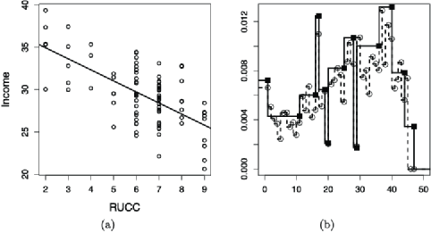
Figure 1: Iowa SEER data: panel (a) shows the scatter plot and simple linear regression line by regressing median household income on RUCC. Panel (b) shows the baseline hazards for Model 1. The dashed line corresponds to Breslow’s estimate of $\lambda_{0}(t)$ obtained by the GF approach, where the circles represent the hazard values at each month; the solid line is the fitted baseline hazard by our approach, where the solid squares correspond to the cut-point values $\mathbf{a}=(1,11,16,17,19,20,25,28,29,36,40,44,47)$.

To get an initial feeling about the role that each county-level covariate is playing, Table 2 provides the distribution of each county-level covariate stratified by the individual-level stage of disease. The gamma statistic (GK), originally proposed by Goodman and Kruskal (1954), is calculated to quantify the association between each county-level covariate and the stage of disease. The GK values range from $-$1 (100% negative association) to $1$ ($100\%$ positive association), where the value $0$ indicates no association. We see that women with a distant-stage at diagnosis are much more likely than those with a local-stage to live in counties with a high degree of urbanization ($\mathrm{GK}=-0.11$; $95\%$ CI: from $-$0.20 to $-$0.01), while the association between stage and income is not significant ($\mathrm{GK}=0.04$; $95\%$ CI: from $-$0.06 to $0.13$). These associations roughly imply that women living in urban counties may suffer poorer survival, assuming that women in distant-stage are more likely to die than women in other stages. Next, we carefully examine both these individual-level and county-level covariates in relation to breast cancer survival, fitting the covariate-adjusted frailty proportional hazards model.

Table 2: Iowa SEER data: Distribution of each county-level covariate stratified by individual-level stage. The pattern of numbers is Number of women (%). Goodman and Kruskal’s gamma statistics (95% confidence intervals) are $-$0.11 $(-0.20,-0.01)$ and $0.04$ $(-0.06,0.13)$ for RUCC and Income, respectively

		Stage
	All women	Local	Regional	Distant
Covariates	$\bolds{N=1073}$	$\bolds{N=510}$	$\bolds{N=355}$	$\bolds{N=208}$
RUCC
1–3	314 (29.3)	131 (25.7)	099 (27.9)	084 (40.4)
4–7	666 (62.1)	342 (67.1)	221 (62.3)	103 (49.5)
8–9	93 (8.6)	37 (7.2)	35 (9.8)	021 (10.1)
Income ($\times$1000)
20–27	163 (15.2)	079 (15.5)	051 (14.4)	033 (15.9)
27–34	651 (60.7)	312 (61.2)	223 (62.8)	116 (55.8)
$>$34	259 (24.1)	119 (23.3)	081 (22.8)	059 (28.3)

3.2 Models and model comparison

We fitted the proposed covariate-adjusted frailty PH model for the Iowa SEER data with different county-level covariates, including models with RUCC only (Model 1), with median household income only (Model 2) and with both (Model 3). To see how the piecewise assumption of baseline hazard affects the predictive ability of models, we considered three specifications of cut-point vector $\mathbf{a}$ as follows: [Case III]

$\mathbf{a}=(1,11,16,17,19,20,25,28,29,36,40,44,47)$, which was determined by visually examining Breslow’s estimate of $\lambda_{0}(t)$ using the GF approach, which is given in panel (b) of Figure 1.

$\mathbf{a}=(3,7,12,16,19,24,29,34,41,47)$, where $a_{k}$ is the $\frac{k}{10}$th quantile of the empirical distribution of observed survival times.

$\mathbf{a}=(47)$, which yields an exponential baseline hazard.

In all cases, we set $J=4$. We fitted all the models using the corresponding variants of the algorithm described in Appendix B of the supplementary material [Zhou et al. (2015)] and similar prior specifications suggested in the simulation study. The Markov chain mixed reasonably well despite the high dimension of our models. For each version of our model and case, we ran a single Markov chain of 1,020,000. A total number of 20,000 were discarded as burn-in period and 10,000 samples were retained for posterior inference. Moreover, we also considered another case II with $13$ cut-points and cut-point specifications based on the event time quantiles from the Kaplan–Meier curve in Appendix E of the supplementary material [Zhou et al. (2015)]. The results show that carefully choosing the cut-points is more important than simply increasing the number of cut-points.

For the sake of comparison, we further fitted the exchangeable MPT frailty Cox model and the Bayesian exchangeable Gaussian frailty Cox model. We compare the models using the log pseudo marginal likelihood (LPML) developed by Geisser and Eddy (1979) and the deviance information criterion (DIC) proposed by Spiegelhalter et al. (2002). In the context of the frailty Cox model, the LPML for model $M$ is defined as $\mathrm{LPML}=\sum_{i=1}^{n}\sum_{j=1}^{n_{i}}\log(\mathrm{CPO}_{ij})$, where $\mathrm{CPO}_{ij}$, the $ij$th conditional predictive ordinate, is given by $[\lambda(t_{ij})^{\delta_{ij}}e^{-\Lambda(t_{ij})}|\mathcal{D}_{(ij)}]$ with $\mathcal{D}_{(ij)}$ denoting the remaining data after excluding the $ij$th data point $\mathcal{D}_{ij}$. One can use the simple method suggested by Gelfand and Dey (1994) to estimate the CPO statistics from MCMC output. A larger value of LPML indicates the corresponding model has better predictive ability. Furthermore, Geisser and Eddy (1979) discussed the exponentiated difference in LPML values from two models to obtain what they termed as a pseudo Bayes factor (PBF). The PBF is a surrogate for the more traditional Bayes factor and can be interpreted similarly, but is more analytically tractable, much less sensitive to prior assumptions, and does not suffer from Lindley’s paradox. Set $\bolds{\Omega}=(\mathbf{e},\bolds{\gamma},\bolds{\beta},\theta)$ as the entire collection of model parameters. The DIC for model $M$ is defined as $\mathrm{DIC}=\bar{D}+p_{D}=E_{\bolds{\Omega}|\mathcal{D}}\{D(\bolds{\Omega})\}+p_{D}$, where $D(\bolds{\Omega})=-2\log\mathcal{L}(\bolds{\gamma},\mathbf{e})$ which is referred to as the deviance function, and $p_{D}=\bar{D}-D(E_{\bolds{\Omega}|\mathcal{D}}\{\bolds{\Omega}\})$ which is a measure of model complexity. Note that the DIC is also readily computed from MCMC output.

3.3 Results

Table 3 shows the DIC and LPML for all models under consideration. All models under case I provide significantly better prediction as measured by both DIC and LPML, with differences in the range of 20–55 for DIC and 10–25 for LPML, which indicates that the determination of the cut-point vector for the baseline hazard plays an important role on model prediction and fit. Comparing the frailty specifications in Model 1 across all cases, the DIC and LPML show the same trend for goodness of fit, with the proposed model based on the LDTFP frailty model outperforming both the MPT and Gaussian models, although the differences are only in the range of 1–4. Comparing between Model 2 and Model 3, the proposed model is always preferred in terms of LPML, while the MPT model is slightly better than others in term of DIC under Model 2. Comparing all the proposed models across Model 1–Model 3, the results indicate that Model 1 always performs best. Overall, allowing the frailty distribution to change with county-level covariates (especially RUCC) does improve model prediction according to LPML. In what follows, we present the results under case I.

Table 3: Iowa SEER data: Deviance information criteria (DIC) and log of the pseudo marginal likelihood (LPML) for models under consideration

		Case I		Case II		Case III
Model	Frailty	DIC	LPML	DIC	LPML	DIC	LPML
1	LDTFP	4436	$-$2222	4463	$-$2234	4495	$-$2247
	MPT	4441	$-$2225	4463	$-$2235	4496	$-$2248
	Gaussian	4444	$-$2225	4467	$-$2236	4497	$-$2248
2	LDTFP	4441	$-$2224	4465	$-$2235	4498	$-$2249
	MPT	4440	$-$2225	4462	$-$2236	4497	$-$2248
	Gaussian	4443	$-$2225	4465	$-$2235	4498	$-$2249
3	LDTFP	4438	$-$2223	4464	$-$2235	4496	$-$2248
	MPT	4441	$-$2225	4464	$-$2235	4498	$-$2249
	Gaussian	4445	$-$2226	4467	$-$2236	4498	$-$2248

Table 4: Iowa SEER data: Posterior medians (95% credible intervals) of fixed effects $\bolds{\xi}$ from various models

Predictor	Model 1	Model 2	Model 3	CAR	Cox
$\xi_{1}$ (Age)	0.019	0.020	0.020	0.018	0.019
	(0.013, 0.025)	(0.014, 0.026)	(0.014, 0.026)	(0.012, 0.025)	(0.013, 0.025)
$\xi_{2}$ (Regional)	0.27	0.27	0.27	0.22	0.30
	(0.03, 0.49)	(0.03, 0.47)	(0.05, 0.50)	(0.01, 0.49)	(0.08, 0.52)
$\xi_{3}$ (Distant)	1.64	1.67	1.65	1.65	1.64
	(1.43, 1.88)	(1.43, 1.89)	(1.43, 1.89)	(1.40, 1.93)	(1.42, 1.87)
$\xi_{x_{1}}$ (RUCC)	$-$0.105		$-$0.082
	($-$0.185, $-$0.041)		($-$0.179, 0.011)
$\xi_{x_{2}}$ (Income)		0.042	0.011
		(0.003, 0.084)	($-$0.040, 0.066)

Table 4 presents posterior medians and equal-tailed $95\%$ credible intervals (CI) for main effects (components of $\bolds{\xi}$) under Model 1–Model 3, with covariate-adjusted frailties, and compares the individual-level covariate effects, that is, ($\xi_{1},\xi_{2},\xi_{3}$), to those obtained by Zhao, Hanson and Carlin (2009), under the standard nonfrailty Cox model and the Cox frailty model that has a MPT prior for the baseline survival, centered at the log-logistic family, and with conditionally autoregressive (CAR) county-level spatial frailties. The best fitting Cox model reported by Zhao, Hanson and Carlin (2009) has an LPML of $-$2226. Therefore, the pseudo Bayes factor for the proposed model versus the CAR model is $e^{2226\mbox{--}2222}\approx 55$, implying that the proposed model predicts about 55 times better than the model with CAR frailties. In addition, the proposed model offers a unique interpretation. The posterior medians and 95% CIs for all individual-level effects change little across the different versions of the proposed model, indicating that the Cox regression estimates are reasonably stable for these data, except for the estimate of “Regional stage,” for which the CAR model 95% CI is much wider than those under the considered versions of the proposed model. This may be partly due to the benefit of including county-level covariates. The best model according to LPML, Model 1, indicates that all the individual-level effects are significant at the 0.05 level. Higher age at diagnosis increases the hazard within each county. For instance, women are about $e^{0.019\times 20}\approx 1.46$ times more likely to die from breast cancer than those twenty years younger who have the same disease stage and live in the same county. Compared with women having local stage of disease, women of the same age and living in the same county are $e^{0.27}\approx 1.31$ times more likely to die if their cancer is detected at the regional stage, and $e^{1.64}\approx 5.16$ times more likely to die if detected at the distant stage. We additionally present the fixed effects under the marginal PH model (i.e., using the R function coxph with option cluster) across Model 1–Model 3 in Appendix E of the supplementary material [Zhou et al. (2015)]. Note that the coefficient estimates under the marginal PH model have population-averaged interpretations and cannot be directly compared with those fitted from the proposed frailty PH model due to different model structures.

Regarding the effect of county-level covariates, living in a higher median household income or urban counties is associated with poorer survival after a breast cancer diagnosis. For example, the results under Model 1 indicate that after controlling for individual covariates and county, the hazard rate of women living in urban counties (with $\mathrm{RUCC}=2$) will be $e^{0.105\times 7}\approx 2$ times larger than that of women in rural counties (with $\mathrm{RUCC}=9$). The results under Model 2 imply that after controlling for individual covariates and frailties, women have about a $1.7$ times larger hazard rate if they live in median household income counties of $35,301 compared with median household income of $23,354 (see also Figure 2). Under Model 3, the results indicate that when both the county-level covariates are included simultaneously, their independent effects are attenuated, partly due to the multicollinearity between them (see the middle two plots in Figure 3).

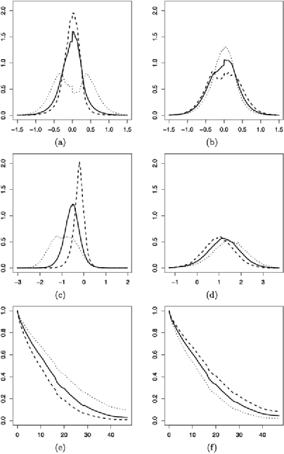
Figure 2: Iowa SEER data: Fitted predictive frailty densities [panels (a) and (b)], frailty densities with location shifts [panels (c) and (d)] and survival curves [panels (e) and (f)] for women with mean entry age 68.8 years and distant stage of disease from different county covariate levels under Model 1 [panels (a), (c) and (e)] and Model 2 [panels (b), (d) and (f)]. In panels (a), (c) and (e), the results for $\mathrm{RUCC}=2$, $5$ and $9$ are displayed as dashed, continuous and dotted lines, respectively. In panels (b), (d) and (f), the results for $\mathrm{Income}=23.354$, $29.176$ and $35.301$ are displayed as dashed, continuous and dotted lines, respectively.

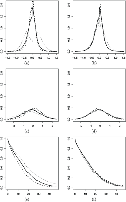
Figure 3: Iowa SEER data: Fitted predictive frailty densities [panels (a) and (b)], frailty densities with location shifts [panels (c) and (d)] and survival curves [panels (e) and (f)] for women with mean entry age 68.8 years and distant stage of disease from different county covariate levels under Model 3. In panels (a), (c) and (e), the results for $\mathrm{RUCC}=2$, $5$ and $9$ are displayed as dashed, continuous and dotted lines, respectively. In panels (b), (d) and (f), the results for $\mathrm{Income}=23.354$, $29.176$ and $35.301$ are displayed as dashed, continuous and dotted lines, respectively.

We obtain the fitted predictive frailty densities for both $\mathbf{e}_{i}$ (median-zero) and $\mathbf{e}_{i}+\mathbf{x}_{i}^{\prime}\bolds{\xi}_{x}$ (full distribution) and survival curves for women with mean entry age $68.8$ years and distant stage of disease who live in the counties with different levels of median household income or RUCC, under the different versions of the proposed model. The three levels are chosen from the 5%, 50% and 95% quantiles of each covariate value. The results are reported in Figures 2 and 3. Under our best fitting, Model 1 (see left three plots in Figure 2), the results indicate that higher values of RUCC increase the frailty variance and suggest a non-Gaussian shape (upper); we also see overall higher frailty after mixing over the location shift $\mathbf{x}_{i}^{\prime}\bolds{\xi}_{x}$ (middle) and so poorer survival (lower) in urban counties. Increasing heterogeneity as ruralness increases under Model 1 translates into increasing association among those living in more rural counties versus urban. In Appendix E of the supplementary material [Zhou et al. (2015)], Kendall’s tau is computed and plotted as a function of RUCC for individuals with mean entry age $68.8$ years and distant stage. Kendall’s tau increases by a factor of three as RUCC goes from 2 to 9. Note that under a traditional gamma frailty model the association is static.

Under Model 2, the frailty densities only slightly change compared with Model 1, but we do see poorer survival in counties with higher median household income. Figure 3 demonstrates that after adjusting individual covariates and median household income (right three plots), there is little effect of RUCC on either predictive frailty densities or survival curves; while after adjusting for RUCC (left three plots), the effect of median household income is almost negligible. In Appendix E of the supplementary material [Zhou et al. (2015)], the survival curves are also compared with those obtained under the marginal PH model. Overall, the marginal PH model under-predicts survival time up to about $1$ month, for example, it gives estimates of median survival a month less, compared with our proposed model for patients with mean entry age $68.8$ years and distant stage of disease who live in the same county. This may be partly due to the fact that the marginal PH model averages over the changing behavior of the frailty distribution over the ruralness measure.

It is widely known that access to quality care and screening for breast cancer is more readily available to those with greater financial means and/or those living in urban areas. Therefore, our findings of increased survival for poorer and more rural counties for this cohort are initially puzzling. However, hormone replacement therapy (HRT) increased about 150% in the 1990s [Wysowski and Governale (2005)], after several observational studies linked HRT to prevention of osteoporosis and protection from heart disease. However, this increasing use of HRT abated suddenly in 2002, when the Women’s Health Initiative clinical trial linked HRT to aggressively invasive breast cancer [Rossouw et al. (2002)]. In fact, overall breast cancer incidence rates peaked in 1999. Between 2001 and 2004 overall invasive breast cancer incidence declined, but fell much more drastically among women living in urban versus rural counties, and among women living in low-poverty versus high-poverty counties. Hausauer et al. (2009) attribute this discrepancy to greater use of postmenopausal estrogen/progestin hormone replacement therapy among more affluent women and/or women living in urban counties up until 2002, when the Women’s Health Initiative trial was stopped prematurely on May 31, 2002, according to Rossouw et al. (2002), “…because the test statistic for invasive breast cancer exceeded the stopping boundary for this adverse effect and the global index statistics supported risks exceeding benefits.” It is plausible that increased risk (i.e., stochastically larger frailties) in more affluent and more urban counties has to do with a larger proportion of women being prescribed HRT in the late 1980s and 1990s. Further exploratory analyses on other cohorts of SEER Iowan breast cancer data (1975–1979, 1980–1984, 1985–1989 and 1990–1994) show a reversal of the effects of income and ruralness, agreeing with intuition. Paralleling our study, Krieger, Chen and Waterman (2010) used county-level census data on income and found rising and falling breast cancer incidence rates for the SEER data over the range 1992–2005 for caucasian women living in high-income counties, which “mirrored the social patterning of hormone therapy use.”

In a longer follow-up study of the Women’s Health Initiative trial, Chlebowski et al. (2010) found that those on estrogen plus progestin compared to placebo had about 25% higher incidence of invasive breast cancer. Among those diagnosed with breast cancer, the two treatment arms had similar histology, but the estrogen plus progestin group were 78% more likely to have cancers that had spread to lymph nodes than placebo, and the estrogen plus progestin group were about twice as likely to die from breast cancer versus placebo. It would appear that hormone replacement therapy fortified the virulence of breast cancer, significantly increasing both incidence and mortality. This same study showed an impressive 7% one-year drop in incidence right after the Women’s Health Initiative study was prematurely stopped and the medical community warned of a possible link between hormone replacement therapy and breast cancer.

4 Simulation studies

We performed a simulation study to assess the performance of the proposed model. The simulated data are also used to compare the proposed approach with existing models. Specifically, we consider the GF approach described in Section 2.1 and the positive stable frailty Cox model proposed by Liu, Kalbfleisch and Schaubel (2011). Under this latter model, the shape parameter is allowed to depend on cluster-level covariates. In terms of our notation, they assumed that the conditional hazard function of $T_{ij}$ is

$$\lambda(t|\tilde{\mathbf{w}}_{ij},\mathbf{x}_{i},e_{i})=\lambda_{0i}(t)\exp\bigl{(}\tilde{\mathbf{w}}_{ij}^{\prime}\tilde{\bolds{\xi}}_{i}+e_{i}\bigr{)},$$ (2)

where the baseline hazard functions $\lambda_{0i}(t)$ and regression parameters $\tilde{\bolds{\xi}}_{i}$ are cluster-specific, and $\exp(e_{i})$ follows a positive stable distribution with shape parameter $\alpha_{i}\in(0,1)$, relying on the cluster-level covariates vector $\mathbf{x}_{i}$ through a logit link function, denoted by $PS(\alpha_{i})$. They did not deal with this model directly, but rather derived the marginal model

$$\lambda(t|\tilde{\mathbf{w}}_{ij},\mathbf{x}_{i})=h_{0}(t)\exp\bigl{(}\tilde{\mathbf{w}}_{ij}^{\prime}\bolds{\eta}\bigr{)}$$ (3)

by imposing the restrictions $\bolds{\eta}=\alpha_{i}\tilde{\bolds{\xi}}_{i}$, $H_{0}(t)=\{\Lambda_{0i}(t)\}^{\alpha_{i}}$, where $H_{0}(t)=\int_{0}^{t}h_{0}(s)\,ds$ and $\Lambda_{0i}=\int_{0}^{t}\lambda_{0i}(s)\,ds$. In other words, they essentially fitted the above marginal Cox model by maximizing the pseudo partial likelihood under the working independence assumption [Wei, Lin and Weissfeld (1989)], and then utilized the imposed constraints to estimate the parameters in the frailty model. Although they considered a more flexible conditional Cox model, they made many assumptions to get the marginal model, some of which are difficult to check in practice. Moreover, they faced a nonidentifiability problem when a cluster-level covariate was included in the conditional Cox model, so cluster-level covariates had to be excluded from the marginal model as well, leading to potentially poorer prediction of the marginal survival function. Their method, referred to below as PSF, will be compared with our approach focusing on the prediction of survival functions in the simulation studies. A comparison of the two methods for the fixed effect estimates cannot be conducted, since they have different model structures. We conducted the simulation study in R. The GF and PSF approaches were implemented by using the function coxme and coxph (with the option cluster), respectively, included in the R packages coxme and survival.

4.1 Simulation settings

Two scenarios for the frailty distributions were considered. In the first case, referred to as Scenario I, a covariate-dependent family of distributions is considered, where the density shape evolves from one mode to two as the cluster-specific covariate $x$ increases its value; this mirrors the effect of RUCC in panel (a) of Figure 3 for Model 1. In the second case, referred to as Scenario II, a covariate-dependent positive stable distribution is considered. The specific distributional forms for each setting were the following: [Scenario II.]

$e_{i}|x_{i}\stackrel{{\scriptstyle\mathrm{ind}.}}{{\sim}}0.5N(-e^{0.4x_{i}},1)+0.5N(e^{0.4x_{i}},1)$, $x_{i}\stackrel{{\scriptstyle\mathrm{i.i.d.}}}{{\sim}}U(-3,3)$.

$\exp(e_{i})|x_{i}\stackrel{{\scriptstyle\mathrm{ind}.}}{{\sim}}PS(\alpha_{i})$, $\alpha_{i}=1/(1+e^{-0.5\mbox{--}0.5x_{i}})$, $x_{i}\stackrel{{\scriptstyle\mathrm{i.i.d.}}}{{\sim}}U(0,2)$. Note that the first setting is not a particular case of the proposed model; the second setting, chosen from the simulation study of Liu, Kalbfleisch and Schaubel (2011), is included to evaluate the behavior of the proposed approach when the PSF model is correct.

Given the frailties, the data under Scenario I were simulated from the conditional PH model (1) with $\lambda_{0}(t)=1$, $\mathbf{w}_{ij}=({w}_{1ij},{w}_{2ij},x_{i})^{\prime}$ and $\bolds{\xi}=(\xi_{1},\xi_{2},\xi_{x})^{\prime}=(1.0,0.5,1.0)^{\prime}$; the data under Scenario II were simulated from the PSF model (2) with $\tilde{\mathbf{w}}_{ij}=(w_{1ij},w_{2ij})^{\prime}$, $\bolds{\eta}=(1,0.5)^{\prime}$ and $H_{0}(t)=t$. For each simulation scenario, $200$ replicates of the data set were generated by assuming the following: $w_{1ij}\stackrel{{\scriptstyle\mathrm{i.i.d.}}}{{\sim}}N(0,1)$ and $w_{2ij}\stackrel{{\scriptstyle\mathrm{i.i.d.}}}{{\sim}}\mbox{Bernoulli}(0.5)$, $i=1,\ldots,100$, $j=1,\ldots,10$. In each case, a noninformative censoring scheme was considered, where the censoring times were simulated from an $U(0.25,4)$ distribution, so that the censoring rate is approximately $35\%$ under Scenario I and $25\%$ under Scenario II.

For each data set, the GF approach was employed, yielding point estimates of $\bolds{\xi}$, $\operatorname{var}(e_{i})$ and $e_{i}$, which we denote by $\hat{\bolds{\xi}}^{(0)}$, $\hat{\theta}^{2(0)}$ and $\hat{e}_{i}^{(0)}$, respectively. Based on these point estimates, the predictive survival function was calculated as follows:

$$\hat{S}_{\mathrm{GF}}(t|\mathbf{w})=n^{-1}\sum_{i=1}^{n}\exp\bigl{\{}-\hat{\Lambda}_{0}^{(0)}(t)\exp\bigl{\{}\mathbf{w}^{\prime}\hat{\bolds{\xi}}^{(0)}+\hat{e}_{i}^{(0)}\bigr{\}}\bigr{\}},$$ (4)

where $\hat{\Lambda}_{0}^{(0)}(t)$, depending on $\hat{e}_{i}^{(0)}$’s, denotes Breslow’s estimator of $\Lambda_{0}(t)$ [see, e.g., Therneau, Grambsch and Pankratz (2003), Section 2]. We then fitted the proposed model, by considering $J=4$, $K=10$, $\tau_{1}=1.001$, $\tau_{2}=1.001\hat{\theta}^{2(0)}$, $a_{c}=1$, $b_{c}=1$, $\bolds{\gamma}_{0}=\mathbf{0}_{13}$ and $\mathbf{S}_{0}=10^{3}\times\mathbf{I}_{13}$. For each data set a single Markov chain of length 55,000 was obtained by using the algorithm described in Appendix B of the supplementary material [Zhou et al. (2015)]. A burn-in period of 5000 scans was considered, and 5000 samples were retained for posterior inferences. The posterior mean of the corresponding parameters are denoted by $\hat{\bolds{\xi}}$, $\hat{\theta}^{2}$, $\hat{g}(e|\mathbf{x})$ and $\hat{S}(t|\mathbf{w})$. Finally, the PSF approach was considered but including the cluster-level covariates in the linear predictor, and the associated predictive survival function, based on Breslow’s estimator of the underlying baseline hazard function, was obtained and is denoted by $\hat{S}_{\mathrm{PSF}}(t|\mathbf{w})$.

The competing approaches were compared regarding the estimation of the regression coefficients and also compared by computing the weighted integrated squared error (ISE) for the estimated survival distributions, given by

$$\int_{0}^{\infty}\bigl{\{}\hat{S}_{m}(t|\mathbf{w})-S(t|\mathbf{w})\bigr{\}}^{2}f_{T}(t|\mathbf{w})\,dt,$$

where $\hat{S}_{m}(t|\mathbf{w})$, $S(t|\mathbf{w})$ and $f_{T}(t|\mathbf{w})$ are the estimated survival function, the true survival function and density function, respectively, for a subject with covariate vector $\mathbf{w}$.

Table 5: Simulation data—Scenario I: True value, bias of the point estimator, mean (across Monte Carlo simulations) of the posterior standard deviations/standard errors (MEAN-SD), standard deviation (across Monte Carlo simulations) of the point estimator (SD-MEAN) and Monte Carlo coverage probability for the $95\%$ credible interval/confidence interval (CP) for the regression parameters. The results are presented under the proposed model and under the GF approach

		Proposed model				GF model
Parameters
	True	BIAS	MEAN-SD	SD-MEAN	CP	BIAS	MEAN-SD	SD-MEAN	CP
$\xi_{1}$	1.0	$-$0.011	0.052	0.054	0.930	$-$0.011	0.051	0.059	0.910
$\xi_{2}$	0.5	$-$0.008	0.088	0.090	0.945	$-$0.003	0.088	0.091	0.950
$\xi_{x}$	1.0	$-$0.009	0.141	0.126	0.965	$-$0.052	0.083	0.142	0.775

4.2 Simulation results

The results for the regression coefficients using the proposed model and the GF approach under Scenario I are given in Table 5, where the bias of the corresponding point estimators, the Monte Carlo mean of the posterior standard deviation/standard error (MEAN-SD), the Monte Carlo standard deviation of the point estimates (SD-MEAN) and the Monte Carlo coverage probability (CP) of the $95\%$ credible interval/confidence intervals are presented. The results suggest that the posterior means of $\bolds{\xi}$ are almost unbiased estimators and that the observed bias for $\xi_{x}$ under the proposed approach is much smaller than the corresponding value obtained under the GF approach. Moreover, under the proposed model, the MEAN-SD and the SD-MEAN values are in fairly close agreement, indicating that the posterior standard deviation is an unbiased estimator of the frequentist standard error. Finally, the CPs are all around the nominal $95\%$. The same does not hold for GF, which substantially underestimates the standard error for $\xi_{x}$, leading to low coverage probabilities.

The average of the estimated frailty distributions and survival functions across simulated data sets for some specific covariate values are presented in Figure 4 for Scenario I and in Figure 5 for Scenario II. The results in Scenario I reveal that the proposed model roughly captures the modal behavior of the covariate-dependent frailty distributions. Although not perfect, the proposed model performs remarkably well given that only $n=100$ imperfectly-observed observations were generated for each data set. The situation is much less favorable for the GF approach, which fails to correctly capture the shape of the frailty distributions, leading to poor estimated survival functions. This behavior is likely driving the underestimation of survival noted in the SEER analysis. As expected, the PSF approach also suffers from bad prediction since the underlying assumption for frailty distribution is violated. The results in Scenario II show that the proposed model is still able to capture the frailty distributional shape even when the data were truly generated from the PSF model. Regarding the estimated survival curves, the results suggest that essentially no differences among the three methods are observed; all estimated functions are close to the truth, indicating that there is little price to be paid when using the proposed model for the clustered survival data that were truly generated from the PSF model.

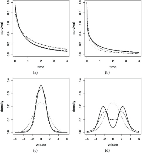
Figure 4: Simulated data—Scenario I: Mean, across simulations, of the posterior mean of the survival and frailty density functions under the proposed model. Panels (a) and (b) show the results for the survival functions. Panels (c) and (d) show the results for the frailty densities. Panels (a) and (c) show the results for covariate values $(2,1,-2)$. Panels (b) and (d) show the results for covariate values $(0,1,~{}2)$. The true curves are represented by continuous lines. The results under the proposed model are represented by dashed lines. The results under the exchangeable Gaussian frailty model are represented by dotted lines. In panels (a) and (b) the results obtained under the PSF approach are represented by dot-dashed lines.

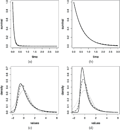
Figure 5: Simulated data—Scenario II: Mean, across simulations, of the posterior mean of the survival and frailty density functions under the proposed model. Panels (a) and (b) show the results for the survival functions. Panels (c) and (d) show the results for the frailty densities. Panels (a) and (c) show the results for covariate values $(2,1,0.5)$. Panels (b) and (d) show the results for covariate values $(0,1,1.5)$. The true curves are represented by continuous lines. The results under the proposed model are represented by dashed lines. The results under the exchangeable Gaussian frailty model are represented by dotted lines. In panels (a) and (b) the results obtained under the PSF approach are represented by dot-dashed lines.

The results of the comparison of the estimated survival curves in terms of ISE are presented in Table 6, where the Monte Carlo mean and standard deviations for the ISE for two different predictor values are given. The results under Scenario I show a close agreement with the observed for the regression coefficients; the proposed model substantially outperforms the other two methods in terms of smaller means and standard deviations of the ISE. Even under Scenario II, the proposed model still provides almost the same results as the PSF model in terms of ISE.

Table 6: Simulated data—Scenario II: Monte Carlo mean (Monte Carlo standard deviation) for the ISE of the survival function for two different predictor values. The results for the different approaches under both simulation scenarios are presented. The numbers correspond to $10^{3}$ times the original values

Scenario	$\bolds{(w_{1},w_{2},x)}$	Proposed model	GF model	PSF model
I	$(2,1,-2)$	2.02 (2.48)	4.37 (3.46)	6.28 (3.49)
	$(0,1,2)$	1.94 (2.53)	10.5 (6.86)	14.3 (10.9)
II	$(2,1,0.5)$	3.17 (4.66)	3.13 (3.33)	2.19 (2.26)
	$(0,1,1.5)$	0.96 (1.18)	0.89 (1.22)	0.83 (1.10)

In Appendix D of the supplementary material [Zhou et al. (2015)], additional simulation results are presented which show that, under Scenario I, for larger sample sizes better estimates of the frailty distributions are obtained and that the approach is not affected by the choice of $J$ in the specification of the LDTFP model. For further comparison, we also fitted the exchangeable mixture of Polya trees (MPT) [Hanson (2006b)] frailty Cox’s model using the function PTglmm available in DPpackage [Jara et al. (2011)] under Scenario I, in which the results show that our approach outperforms the MPT, and considered a third scenario favorable to the GP approach, where the results show that our method pays little price for the extra generality when using the proposed model when normality and exchangeability are valid assumptions. Overall, the proposed approach provides a flexible way to capture the heterogeneity in the frailty distribution, provides superior prediction, and yields an essential improvement for the estimation of population effects, especially when the intra-cluster correlation (or variability in frailties) is relatively large. When the frailty variances are small across clusters, the proposed approach is still recommended due to its flexibility.

5 Concluding remarks

Very limited work has been done on covariate-adjusted frailty survival models for clustered time-to-event data. Liu,Kalbfleisch and Schaubel (2011) proposed a stratified Cox model with positive stable frailties, where the shape parameter of the frailty distribution is allowed to depend on cluster-level covariates. However, they essentially fitted a marginal Cox model, and then utilized the positive stable assumption and some imposed constraints to estimate the parameters in their proposed model. The model proposed in this paper cleanly separates population-level effects from the cluster-level effects, which determine the shape of the frailty distribution. Frailty density shape is modeled using a tractable median-zero LDTFP prior. Other nonparametric density regression approaches could also be considered; however, model identifiability requires a location constraint such as mean-zero or median-zero. The proposed model provides a natural generalization of the conventional PH model with parametric or nonparametric exchangeable frailties, and accommodates frailty distribution “evolution” over cluster-level covariates providing superior prediction, as shown in our simulation studies. When data are truly generated according to an exchangeable Gaussian frailty PH model or the model of Liu, Kalbfleisch and Schaubel (2011), our model does about the same as the underlying true model in terms of fixed effects and/or marginal survival estimations. We illustrate the usefulness of the proposed model with an analysis of a subset of the Iowa SEER breast cancer data, and demonstrate that higher degree of ruralness corresponds to a more bimodal frailty distributional shape with larger variance. In general, the proposed model is more flexible than currently existing frailty PH models, leading to more robust inferences, and thus is recommended. One drawback of the proposed model is that, as currently fit in R, obtaining inference takes longer.

For ease of computation, we have assumed a piecewise constant structure for the baseline hazard function $\lambda_{0}(t)$ and taken the independent normal prior distributions for $\log(\lambda_{k})$’s, so that the baseline hazard heights $\lambda_{k}$ and covariate effects $\bolds{\xi}$ can be updated simultaneously. The use of empirically-derived cut-points has permeated much of the Bayesian survival literature for over a decade. Use of Breslow’s baseline estimate coupled with the GF approach led to a greatly increased LPML over the empirical approach. An obvious extension of our current work is to employ a smoothed baseline, for example, using penalized B-splines [Hennerfeind, Brezger and Fahrmeir (2006)], the piecewise exponential with random cut-points [Sahu and Dey (2004)], MPT [Hanson (2006b)], etc. Any of these approaches could improve model fit and prediction, but cannot currently be fitted in the R software. We are currently working on extending the methodology in this paper to other survival models and smoothed baselines.

References

- Chlebowski et al. (2010) {barticle}[author] \bauthor\bsnmChlebowski, \bfnmRowan T.\binitsR. T., \bauthor\bsnmAnderson, \bfnmGarnet L.\binitsG. L., \bauthor\bsnmGass, \bfnmMargery\binitsM., \bauthor\bsnmLane, \bfnmDorothy S.\binitsD. S., \bauthor\bsnmAragaki, \bfnmAaron K.\binitsA. K., \bauthor\bsnmKuller, \bfnmLewis H.\binitsL. H., \bauthor\bsnmManson, \bfnmJoAnn E.\binitsJ. E., \bauthor\bsnmStefanick, \bfnmMarcia L.\binitsM. L., \bauthor\bsnmOckene, \bfnmJudith\binitsJ., \bauthor\bsnmSarto, \bfnmGloria E.\binitsG. E. \betalet al. (\byear2010). \btitleEstrogen plus progestin and breast cancer incidence and mortality in postmenopausal women. \bjournalJAMA \bvolume304 \bpages1684–1692. \bptokimsref\endbibitem
- Clayton and Cuzick (1985) {barticle}[mr] \bauthor\bsnmClayton, \bfnmDavid\binitsD. and \bauthor\bsnmCuzick, \bfnmJack\binitsJ. (\byear1985). \btitleMultivariate generalizations of the proportional hazards model. \bjournalJ. Roy. Statist. Soc. Ser. A \bvolume148 \bpages82–117. \biddoi=10.2307/2981943, issn=0035-9238, mr=0806480 \bptokimsref\endbibitem
- Cottone (2008) {bmisc}[author] \bauthor\bsnmCottone, \bfnmFrancesco\binitsF. (\byear2008). \bhowpublishedCovariate dependent random effects in survival analysis, Ph.D. dissertation, Univ. degli Studi “Roma Tre.” \bptokimsref\endbibitem
- Geisser and Eddy (1979) {barticle}[mr] \bauthor\bsnmGeisser, \bfnmSeymour\binitsS. and \bauthor\bsnmEddy, \bfnmWilliam F.\binitsW. F. (\byear1979). \btitleA predictive approach to model selection. \bjournalJ. Amer. Statist. Assoc. \bvolume74 \bpages153–160. \bidissn=0003-1291, mr=0529531 \bptokimsref\endbibitem
- Gelfand and Dey (1994) {barticle}[mr] \bauthor\bsnmGelfand, \bfnmA. E.\binitsA. E. and \bauthor\bsnmDey, \bfnmD. K.\binitsD. K. (\byear1994). \btitleBayesian model choice: Asymptotics and exact calculations. \bjournalJ. Roy. Statist. Soc. Ser. B \bvolume56 \bpages501–514. \bidissn=0035-9246, mr=1278223 \bptokimsref\endbibitem
- Goodman and Kruskal (1954) {barticle}[author] \bauthor\bsnmGoodman, \bfnmLeo A.\binitsL. A. and \bauthor\bsnmKruskal, \bfnmWilliam H.\binitsW. H. (\byear1954). \btitleMeasures of association for cross classifications. \bjournalJ. Amer. Statist. Assoc. \bvolume49 \bpages732–764. \bptokimsref\endbibitem
- Gustafson (1997) {barticle}[pbm] \bauthor\bsnmGustafson, \bfnmP.\binitsP. (\byear1997). \btitleLarge hierarchical Bayesian analysis of multivariate survival data. \bjournalBiometrics \bvolume53 \bpages230–242. \bidissn=0006-341X, pmid=9147593 \bptokimsref\endbibitem
- Hanson (2006a) {barticle}[mr] \bauthor\bsnmHanson, \bfnmTimothy E.\binitsT. E. (\byear2006a). \btitleInference for mixtures of finite Polya tree models. \bjournalJ. Amer. Statist. Assoc. \bvolume101 \bpages1548–1565. \biddoi=10.1198/016214506000000384, issn=0162-1459, mr=2279479 \bptokimsref\endbibitem
- Hanson (2006b) {barticle}[mr] \bauthor\bsnmHanson, \bfnmTimothy E.\binitsT. E. (\byear2006b). \btitleModeling censored lifetime data using a mixture of gammas baseline. \bjournalBayesian Anal. \bvolume1 \bpages575–593 (electronic). \bidmr=2221289 \bptokimsref\endbibitem
- Hanson, Johnson and Laud (2009) {barticle}[mr] \bauthor\bsnmHanson, \bfnmTimothy\binitsT., \bauthor\bsnmJohnson, \bfnmWesley\binitsW. and \bauthor\bsnmLaud, \bfnmPurushottam\binitsP. (\byear2009). \btitleSemiparametric inference for survival models with step process covariates. \bjournalCanad. J. Statist. \bvolume37 \bpages60–79. \biddoi=10.1002/cjs.10001, issn=0319-5724, mr=2509462 \bptokimsref\endbibitem
- Hausauer et al. (2009) {barticle}[author] \bauthor\bsnmHausauer, \bfnmAmelia K.\binitsA. K., \bauthor\bsnmKeegan, \bfnmTheresa HM\binitsT. H., \bauthor\bsnmChang, \bfnmEllen T.\binitsE. T., \bauthor\bsnmGlaser, \bfnmSally L.\binitsS. L., \bauthor\bsnmHowe, \bfnmHolly\binitsH. and \bauthor\bsnmClarke, \bfnmChristina A.\binitsC. A. (\byear2009). \btitleRecent trends in breast cancer incidence in US white women by county-level urban/rural and poverty status. \bjournalBMC Medicine \bvolume7 \bpages31. \bptokimsref\endbibitem
- Hennerfeind, Brezger and Fahrmeir (2006) {barticle}[mr] \bauthor\bsnmHennerfeind, \bfnmAndrea\binitsA., \bauthor\bsnmBrezger, \bfnmAndreas\binitsA. and \bauthor\bsnmFahrmeir, \bfnmLudwig\binitsL. (\byear2006). \btitleGeoadditive survival models. \bjournalJ. Amer. Statist. Assoc. \bvolume101 \bpages1065–1075. \biddoi=10.1198/016214506000000348, issn=0162-1459, mr=2324146 \bptokimsref\endbibitem
- Jara and Hanson (2011) {barticle}[mr] \bauthor\bsnmJara, \bfnmA.\binitsA. and \bauthor\bsnmHanson, \bfnmT. E.\binitsT. E. (\byear2011). \btitleA class of mixtures of dependent tail-free processes. \bjournalBiometrika \bvolume98 \bpages553–566. \biddoi=10.1093/biomet/asq082, issn=0006-3444, mr=2836406 \bptokimsref\endbibitem
- Jara et al. (2011) {barticle}[author] \bauthor\bsnmJara, \bfnmA.\binitsA., \bauthor\bsnmHanson, \bfnmT. E.\binitsT. E., \bauthor\bsnmQuintana, \bfnmF. A.\binitsF. A., \bauthor\bsnmMüller, \bfnmP.\binitsP. and \bauthor\bsnmRosner, \bfnmG. L.\binitsG. L. (\byear2011). \btitleDPpackage: Bayesian semi- and nonparametric modeling in R. \bjournalJ. Stat. Softw. \bvolume40 \bpages1. \bptokimsref\endbibitem
- Kalbfleisch (1978) {barticle}[mr] \bauthor\bsnmKalbfleisch, \bfnmJohn D.\binitsJ. D. (\byear1978). \btitleNon-parametric Bayesian analysis of survival time data. \bjournalJ. Roy. Statist. Soc. Ser. B \bvolume40 \bpages214–221. \bidissn=0035-9246, mr=0517442 \bptokimsref\endbibitem
- Krieger, Chen and Waterman (2010) {barticle}[author] \bauthor\bsnmKrieger, \bfnmN.\binitsN., \bauthor\bsnmChen, \bfnmJ T.\binitsJ. T. and \bauthor\bsnmWaterman, \bfnmP D.\binitsP. D. (\byear2010). \btitleDecline in US breast cancer rates after the women’s health initiative: Socioeconomic and racial/ethnic differentials. \bjournalAmerican Journal of Public Health \bvolume100 \bpages132–139. \bptokimsref\endbibitem
- Laird and Olivier (1981) {barticle}[mr] \bauthor\bsnmLaird, \bfnmNan\binitsN. and \bauthor\bsnmOlivier, \bfnmDonald\binitsD. (\byear1981). \btitleCovariance analysis of censored survival data using log-linear analysis techniques. \bjournalJ. Amer. Statist. Assoc. \bvolume76 \bpages231–240. \bidissn=0003-1291, mr=0624329 \bptokimsref\endbibitem
- Liu, Kalbfleisch and Schaubel (2011) {barticle}[mr] \bauthor\bsnmLiu, \bfnmDandan\binitsD., \bauthor\bsnmKalbfleisch, \bfnmJohn D.\binitsJ. D. and \bauthor\bsnmSchaubel, \bfnmDouglas E.\binitsD. E. (\byear2011). \btitleA positive stable frailty model for clustered failure time data with covariate-dependent frailty. \bjournalBiometrics \bvolume67 \bpages8–17. \biddoi=10.1111/j.1541-0420.2010.01444.x, issn=0006-341X, mr=2898812 \bptokimsref\endbibitem
- McCulloch and Neuhaus (2011) {barticle}[mr] \bauthor\bsnmMcCulloch, \bfnmCharles E.\binitsC. E. and \bauthor\bsnmNeuhaus, \bfnmJohn M.\binitsJ. M. (\byear2011). \btitleMisspecifying the shape of a random effects distribution: Why getting it wrong may not matter. \bjournalStatist. Sci. \bvolume26 \bpages388–402. \biddoi=10.1214/11-STS361, issn=0883-4237, mr=2917962 \bptokimsref\endbibitem
- Noh, Ha and Lee (2006) {barticle}[mr] \bauthor\bsnmNoh, \bfnmMaengseok\binitsM., \bauthor\bsnmHa, \bfnmIl Do\binitsI. D. and \bauthor\bsnmLee, \bfnmYoungjo\binitsY. (\byear2006). \btitleDispersion frailty models and HGLMs. \bjournalStat. Med. \bvolume25 \bpages1341–1354. \biddoi=10.1002/sim.2284, issn=0277-6715, mr=2226790 \bptokimsref\endbibitem
- Qiou, Ravishanker and Dey (1999) {barticle}[pbm] \bauthor\bsnmQiou, \bfnmZ.\binitsZ., \bauthor\bsnmRavishanker, \bfnmN.\binitsN. and \bauthor\bsnmDey, \bfnmD. K.\binitsD. K. (\byear1999). \btitleMultivariate survival analysis with positive stable frailties. \bjournalBiometrics \bvolume55 \bpages637–644. \bidissn=0006-341X, pmid=11318227 \bptokimsref\endbibitem
- Reich, Bondell and Wang (2010) {barticle}[pbm] \bauthor\bsnmReich, \bfnmBrian J.\binitsB. J., \bauthor\bsnmBondell, \bfnmHoward D.\binitsH. D. and \bauthor\bsnmWang, \bfnmHuixia J.\binitsH. J. (\byear2010). \btitleFlexible Bayesian quantile regression for independent and clustered data. \bjournalBiostatistics \bvolume11 \bpages337–352. \biddoi=10.1093/biostatistics/kxp049, issn=1468-4357, pii=kxp049, pmid=19948746 \bptokimsref\endbibitem
- Rossouw et al. (2002) {barticle}[pbm] \bauthor\bsnmRossouw, \bfnmJacques E.\binitsJ. E., \bauthor\bsnmAnderson, \bfnmGarnet L.\binitsG. L., \bauthor\bsnmPrentice, \bfnmRoss L.\binitsR. L., \bauthor\bsnmLaCroix, \bfnmAndrea Z.\binitsA. Z., \bauthor\bsnmKooperberg, \bfnmCharles\binitsC., \bauthor\bsnmStefanick, \bfnmMarcia L.\binitsM. L., \bauthor\bsnmJackson, \bfnmRebecca D.\binitsR. D., \bauthor\bsnmBeresford, \bfnmShirley A. A.\binitsS. A. A., \bauthor\bsnmHoward, \bfnmBarbara V.\binitsB. V., \bauthor\bsnmJohnson, \bfnmKaren C.\binitsK. C., \bauthor\bsnmKotchen, \bfnmJane Morley\binitsJ. M. and \bauthor\bsnmOckene, \bfnmJudith\binitsJ. (\byear2002). \btitleRisks and benefits of estrogen plus progestin in healthy postmenopausal women: Principal results from the women’s health initiative randomized controlled trial. \bjournalJAMA \bvolume288 \bpages321–333. \bidissn=0098-7484, pii=joc21036, pmid=12117397 \bptokimsref\endbibitem
- Sahu and Dey (2004) {bincollection}[author] \bauthor\bsnmSahu, \bfnmSujit K.\binitsS. K. and \bauthor\bsnmDey, \bfnmDipak K.\binitsD. K. (\byear2004). \btitleOn a Bayesian multivariate survival model with a skewed frailty. In \bbooktitleSkew-Elliptical Distributions and Their Applications: A Journey Beyond Normality (\beditor\bfnmM. G.\binitsM. G. \bsnmGenton, ed.) \bpages321–338. \bpublisherChapman&Hall/CRC, \blocationBoca Raton, FL. \bptokimsref\endbibitem
- Spiegelhalter et al. (2002) {barticle}[mr] \bauthor\bsnmSpiegelhalter, \bfnmDavid J.\binitsD. J., \bauthor\bsnmBest, \bfnmNicola G.\binitsN. G., \bauthor\bsnmCarlin, \bfnmBradley P.\binitsB. P. and \bauthor\bsnmvan der Linde, \bfnmAngelika\binitsA. (\byear2002). \btitleBayesian measures of model complexity and fit. \bjournalJ. R. Stat. Soc. Ser. B Stat. Methodol. \bvolume64 \bpages583–639. \biddoi=10.1111/1467-9868.00353, issn=1369-7412, mr=1979380 \bptokimsref\endbibitem
- Sprague et al. (2011) {barticle}[pbm] \bauthor\bsnmSprague, \bfnmBrian L.\binitsB. L., \bauthor\bsnmTrentham-Dietz, \bfnmAmy\binitsA., \bauthor\bsnmGangnon, \bfnmRonald E.\binitsR. E., \bauthor\bsnmRamchandani, \bfnmRitesh\binitsR., \bauthor\bsnmHampton, \bfnmJohn M.\binitsJ. M., \bauthor\bsnmRobert, \bfnmStephanie A.\binitsS. A., \bauthor\bsnmRemington, \bfnmPatrick L.\binitsP. L. and \bauthor\bsnmNewcomb, \bfnmPolly A.\binitsP. A. (\byear2011). \btitleSocioeconomic status and survival after an invasive breast cancer diagnosis. \bjournalCancer \bvolume117 \bpages1542–1551. \biddoi=10.1002/cncr.25589, issn=0008-543X, mid=NIHMS225856, pmcid=3116955, pmid=21425155 \bptokimsref\endbibitem
- Therneau and Grambsch (2000) {bbook}[mr] \bauthor\bsnmTherneau, \bfnmTerry M.\binitsT. M. and \bauthor\bsnmGrambsch, \bfnmPatricia M.\binitsP. M. (\byear2000). \btitleModeling Survival Data: Extending the Cox Model. \bpublisherSpringer, \blocationNew York. \biddoi=10.1007/978-1-4757-3294-8, mr=1774977 \bptokimsref\endbibitem
- Therneau, Grambsch and Pankratz (2003) {barticle}[mr] \bauthor\bsnmTherneau, \bfnmTerry M.\binitsT. M., \bauthor\bsnmGrambsch, \bfnmPatricia M.\binitsP. M. and \bauthor\bsnmPankratz, \bfnmV. Shane\binitsV. S. (\byear2003). \btitlePenalized survival models and frailty. \bjournalJ. Comput. Graph. Statist. \bvolume12 \bpages156–175. \biddoi=10.1198/1061860031365, issn=1061-8600, mr=1965213 \bptokimsref\endbibitem
- Trippa, Müller and Johnson (2011) {barticle}[mr] \bauthor\bsnmTrippa, \bfnmLorenzo\binitsL., \bauthor\bsnmMüller, \bfnmPeter\binitsP. and \bauthor\bsnmJohnson, \bfnmWesley\binitsW. (\byear2011). \btitleThe multivariate beta process and an extension of the Polya tree model. \bjournalBiometrika \bvolume98 \bpages17–34. \biddoi=10.1093/biomet/asq072, issn=0006-3444, mr=2804207 \bptokimsref\endbibitem
- Vaupel, Manton and Stallard (1979) {barticle}[author] \bauthor\bsnmVaupel, \bfnmJames W.\binitsJ. W., \bauthor\bsnmManton, \bfnmKenneth G.\binitsK. G. and \bauthor\bsnmStallard, \bfnmEric\binitsE. (\byear1979). \btitleThe impact of heterogeneity in individual frailty on the dynamics of mortality. \bjournalDemography \bvolume16 \bpages439–454. \bptokimsref\endbibitem
- Walker and Mallick (1997) {barticle}[mr] \bauthor\bsnmWalker, \bfnmStephen G.\binitsS. G. and \bauthor\bsnmMallick, \bfnmBani K.\binitsB. K. (\byear1997). \btitleHierarchical generalized linear models and frailty models with Bayesian nonparametric mixing. \bjournalJ. Roy. Statist. Soc. Ser. B \bvolume59 \bpages845–860. \biddoi=10.1111/1467-9868.00101, issn=0035-9246, mr=1483219 \bptokimsref\endbibitem
- Wang and Louis (2004) {barticle}[mr] \bauthor\bsnmWang, \bfnmZengri\binitsZ. and \bauthor\bsnmLouis, \bfnmThomas A.\binitsT. A. (\byear2004). \btitleMarginalized binary mixed-effects models with covariate-dependent random effects and likelihood inference. \bjournalBiometrics \bvolume60 \bpages884–891. \biddoi=10.1111/j.0006-341X.2004.00243.x, issn=0006-341X, mr=2133540 \bptokimsref\endbibitem
- Wassell and Moeschberger (1993) {barticle}[author] \bauthor\bsnmWassell, \bfnmJames T.\binitsJ. T. and \bauthor\bsnmMoeschberger, \bfnmM. L.\binitsM. L. (\byear1993). \btitleA bivariate survival model with modified gamma frailty for assessing the impact of interventions. \bjournalStat. Med. \bvolume12 \bpages241–248. \bptokimsref\endbibitem
- Wei, Lin and Weissfeld (1989) {barticle}[mr] \bauthor\bsnmWei, \bfnmL. J.\binitsL. J., \bauthor\bsnmLin, \bfnmD. Y.\binitsD. Y. and \bauthor\bsnmWeissfeld, \bfnmL.\binitsL. (\byear1989). \btitleRegression analysis of multivariate incomplete failure time data by modeling marginal distributions. \bjournalJ. Amer. Statist. Assoc. \bvolume84 \bpages1065–1073. \bidissn=0162-1459, mr=1134494 \bptokimsref\endbibitem
- Wysowski and Governale (2005) {barticle}[author] \bauthor\bsnmWysowski, \bfnmDiane K.\binitsD. K. and \bauthor\bsnmGovernale, \bfnmLaura A.\binitsL. A. (\byear2005). \btitleUse of menopausal hormones in the United States, 1992 through June, 2003. \bjournalPharmacoepidemiology and Drug Safety \bvolume14 \bpages171–176. \bptokimsref\endbibitem
- Yashin and Iachine (1999) {barticle}[mr] \bauthor\bsnmYashin, \bfnmAnatoli I.\binitsA. I. and \bauthor\bsnmIachine, \bfnmIvan A.\binitsI. A. (\byear1999). \btitleWhat difference does the dependence between durations make? Insights for population studies of aging. \bjournalLifetime Data Anal. \bvolume5 \bpages5–22. \biddoi=10.1023/A:1009622214567, issn=1380-7870, mr=1750339 \bptokimsref\endbibitem
- Zhao and Hanson (2011) {barticle}[mr] \bauthor\bsnmZhao, \bfnmLuping\binitsL. and \bauthor\bsnmHanson, \bfnmTimothy E.\binitsT. E. (\byear2011). \btitleSpatially dependent Polya tree modeling for survival data. \bjournalBiometrics \bvolume67 \bpages391–403. \biddoi=10.1111/j.1541-0420.2010.01468.x, issn=0006-341X, mr=2829008 \bptokimsref\endbibitem
- Zhao, Hanson and Carlin (2009) {barticle}[mr] \bauthor\bsnmZhao, \bfnmLuping\binitsL., \bauthor\bsnmHanson, \bfnmTimothy E.\binitsT. E. and \bauthor\bsnmCarlin, \bfnmBradley P.\binitsB. P. (\byear2009). \btitleMixtures of Polya trees for flexible spatial frailty survival modelling. \bjournalBiometrika \bvolume96 \bpages263–276. \biddoi=10.1093/biomet/asp014, issn=0006-3444, mr=2507142 \bptokimsref\endbibitem
- Zhou et al. (2015) {bmisc}[author] \bauthor\bsnmZhou, \binitsH., \bauthor\bsnmHanson, \binitsT., \bauthor\bsnmJara, \binitsA. and \bauthor\bsnmZhang, \binitsJ. (\byear2015). \bhowpublishedSupplement to “Modeling county level breast cancer survival data using a covariate-adjusted frailty proportional hazards model.” DOI:\doiurl10.1214/14-AOAS793SUPP. \bptokimsref \bptokimsref\endbibitem