Regularity and chaos in $0^{+}$ states of the interacting boson model using quantum measures

Abstract

Background: Statistical measures of chaos have long been used in the study of chaotic dynamics in the framework of the interacting boson model. The use of large number of bosons renders additional studies of chaos possible, that can provide a direct comparison with similar classical studies of chaos.

Purpose: We intend to provide complete quantum chaotic dynamics at zero angular momentum in the vicinity of the arc of regularity and link the results of the study of chaos using statistical measures with those of the study of chaos using classical measures.

Method: Statistical measures of chaos are applied on the spectrum and the transition intensities of $0^{+}$ states in the framework of the interacting boson model.

Results: The energy dependence of chaos is provided for the first time using statistical measures of chaos. The position of the arc of regularity was also found to be stable in the limit of large boson numbers.

Conclusions: The results of the study of chaos using statistical measures are consistent with previous studies using classical measures of chaos, as well as with studies using statistical measures of chaos, but for small number of bosons and states with angular momentum greater than 2.

I Introduction

The Interacting Boson Model (IBM) IA , apart from being successful in describing the low-lying levels and electromagnetic transition intensities of even-even heavy nuclei, has also been used in studying transitions JPG ; RMP between the different dynamical symmetries of the model, by changing its parameters. The model is known to possess 3 dynamical symmetries, namely U(5), O(6) and SU(3). When a system possesses a certain dynamical symmetry, it is completely integrable. Away from these dynamical symmetries, one would expect chaos. However, this is not always the case. A situation of great interest is the notion of quasidynamical symmetry (QDS), i.e., the approximate persistence of a symmetry, in spite of strong symmetry breaking interactions Rowe1225 ; Rowe2325 ; Rowe745 ; Rowe756 ; Rowe759 . Symmetry breaking can also be seen as the transition of a system from regular dynamics (exhibited by the presence of a dynamical symmetry) to chaos Gutzwiller ; Haake .

The interplay between regular and chaotic behavior in the context of the Interacting Boson Model (IBM), has been extensively studied by Alhassid and Whelan Alha4 ; Alha5 ; Alha6 ; Whe1 ; Whe2 and other authors Liu , using both classical and quantum measures of chaos. In their study, they had found integrability at the three dynamical symmetry limits of the symmetry triangle triangle of the IBM, namely, U(5), O(6) and SU(3), as well as at the O(6)–U(5) side of the triangle, due to the O(5) symmetry known Talmi to underlie the O(6)–U(5) line. Away from these integrable regions, one expected chaotic behavior. However, the study of the interior of the symmetry triangle of the IBM, brought to the surface a region of nearly regular behavior Alha5 ; Whe1 ; Whe2 , connecting the U(5) and SU(3) vertices, known as the “Alhassid–Whelan arc of regularity” (AW arc).

The increased regularity observed in the region of the Alhassid–Whelan arc, as well as the locus of the arc, have been studied using several different techniques.

1) Information entropy of the wavefunctions is a measure that quantifies the eigenstate localization of a particular IBM Hamiltonian in different symmetry bases associated with dynamical symmetries, linking it with the degree of regularity Cejn1 ; Cejn2 . It has indeed been found Cejn1 ; Cejn2 that increased localization in the symmetry bases occurs on the Alhassid–Whelan arc of regularity.

2) The line corresponding to the degeneracy of the $0_{2}^{+}$ and $2_{2}^{+}$ states within the symmetry triangle of the IBM has been found to closely follow the arc of regularity Jolie ; Amon . Furthermore, more than twelve nuclei exhibiting this behavior were placed on the arc, providing an experimental confirmation of its existence Jolie ; Amon . Later on, the approximate degeneracy of the $0_{2}^{+}$ and $2_{2}^{+}$ states has been related to the degeneracy of the $\beta$ and $\gamma$ bandheads, its locus has been determined through the intrinsic state formalism, and has been found to be located very close to the Alhassid–Whelan arc Macek2 ; Macek80 .

3) The dynamics of $0^{+}$ states have also been considered, using the nearest neighbor spacing distribution of $0^{+}$ states, in order to demonstrate the semiregular nature of the arc of regularity, in agreement with results obtained using classical measures based on Poincaré sections Macek2 . In particular, a bunching pattern of $0^{+}$ states has been found Macek2 on the arc, similar to the bunching pattern seen along the O(6)–U(5) side of the triangle Heinze , which is known for its regular dynamics Talmi .

4) The line corresponding to the degeneracy of the $2_{\beta}^{+}$ and $2_{\gamma}^{+}$ states has also been found Bon1 to closely follow the arc of regularity. In the large boson number limit this degeneracy also guarantees the degeneracies predicted by the SU(3) symmetry in the first few bands lying lowest in energy. This can be considered Bon1 as a sign of an underlying SU(3) quasidynamical symmetry, however its validity is limited to low lying states and to the large boson number limit.

5) A line within the symmetry triangle of the IBM, also lying close to the arc of regularity, has been obtained Bon2 using a contraction of the SU(3) algebra to the algebra of the rigid rotator. This finding is related to the ground state band alone and has again been obtained in the limit of large boson numbers.

6) Recently, families of high-lying regular rotational bands have been found Macek3 ; Macek4 in the IBM framework, occurring even in nuclei far away from the SU(3) dynamical symmetry and leading to increased overall regularity.

The present paper offers a closer view on the quantum chaotic dynamics at the vicinity of the arc of regulatiry, without attempting to elucidate the nature of the symmetry underlying the arc. Taking advantage of the new code IBAR IBAR1 ; IBAR2 , which can handle up to $N_{B}=1000$ bosons, the present study is focused on states with zero angular momentum ($J=0$), but can be easily extended to other angular momentum values. The main objectives are described here.

1) To determine any energy dependence of statistical measures of quantum chaos in $0^{+}$ states and in $B(E0)$ transition strengths. This study is for the first time feasible, due to the good statistics allowed by the large number of bosons used.

2) To examine the stability of the location of the arc of regularity within the symmetry trianlge of IBM with changing boson number. The IBAR code allows for the first time to examine this stability for large boson numbers. The question of stability is of importance in relation to the empirical evidence Jolie ; Amon found for the arc of regularity, since different nuclei are described by different boson numbers, in the region of deformed nuclei already used Jolie ; Amon the boson number being close to 14.

In Section II, the IBM Hamiltonian is described. The fluctuation measures, used to study the quantum dynamics in the symmetry triangle of the IBM are introduced in Section III, while in Section IV the numerical results are presented. An O(6) line is considered in Section V, while in Section VI the discussion of the results is given.

II IBM Hamiltonian and symmetry triangle

In the context of the IBM, low lying states in nuclei can be described in terms of a monopole boson, $s$, with angular momentum 0 and a quadrupole boson, $d$, with angular momentum 2. The 36 bilinear combinations ($s^{{\dagger}}s,\;s^{{\dagger}}\tilde{d}_{\mu},\;d^{{\dagger}}_{\mu}s,\;d^{{\dagger}}_{\mu}\tilde{d}_{\nu}$) form a U(6) spectrum generating algebra. The three dynamical symmetries of the model, U(5), SU(3) and O(6), which correspond to vibrational, rotational, and $\gamma$–unstable nuclei, respectively, are placed at the vertices of the symmetry triangle, shown in Figure 1, which is the parameter space of the model.

In what follows we use the IBM Hamiltonian Alha5 ; Whe1 ; Whe2 ,

$$H\left(\eta,\chi\right)=c\left[\eta\hat{n}_{d}+\frac{\eta-1}{N_{B}}\hat{Q}_{\chi}\cdot\hat{Q}_{\chi}\right],$$ (1)

where $\hat{n}_{d}=d^{{\dagger}}\cdot\tilde{d}$ is the d boson number operator, $\hat{Q}_{\chi}=(s^{{\dagger}}\tilde{d}+d^{{\dagger}}s)+\chi(d^{{\dagger}}\tilde{d})^{(2)}$ is the quadrupole operator, and $N_{B}$ is the number of valence bosons. The parameters $(\eta,\chi)$ are the coordinates of the triangle and serve for symmetry breaking. $\eta$ ranges from 0 to 1, and $\chi$ ranges from 0 to $\frac{-\sqrt{7}}{2}\approx-1.32$. By varying $\eta$ and $\chi$, the three dynamical symmetries of the model can be reached. U(5) corresponds to $(\eta,\chi)=(1,0)$, O(6) to $(\eta,\chi)=(0,0)$ and SU(3) to $(\eta,\chi)=(0,\frac{-\sqrt{7}}{2})$. Numerical calculations of energy levels and $B(E0)$ transition rates have been performed using the code IBAR IBAR1 ; IBAR2 which can handle up to $N_{B}$=1000 bosons.

III Fluctuation measures

In this section, the fluctuation measures or statistics, which are applied to the spectrum and the transition intensities of $0^{+}$ states, are introduced. However, before proceeding to the quantum chaotic analysis of the spectrum or of the transitions intensities, the eigenvalues should be unfolded. The reason is that the Gaussian Orthogonal Ensemble (GOE) requires that the average level spacing, $S$, of a spectrum in the limit $N\rightarrow\infty$ should be constant, however, the ordered sequence of levels $(E_{1},E_{2},\dots,E_{N})$ produced, for example from the IBM Hamiltonian, forms a spectrum in which the low energy levels have consistently larger spacings than the high energy ones. In order to be consistent with the GOE requirements, one needs to unfold the spectra, that is to say, modify the spectrum, so that the average level spacing, $S$, is constant. The first step of unfolding is performed by constructing a staircase function of the data. A staircase function is the number of levels found below some specific energy. Then, a low order polynomial $N(E)$ is fitted to the staircase function Alha1 . The unfolded energies, called normalized energies, are defined as $\epsilon_{i}=N(E_{i})$. With this mapping, the average level spacing of the spectrum of the normalized energies, the unfolded spectrum, becomes constant and specifically, equal to one, $\langle S\rangle=1$. The fluctuation measures, are then applied to the unfolded spectrum, which might have constant average level spacing, however, the spacings still show strong fluctuations.

The statistical measures used for the determination of the fluctuation properties of the unfolded spectrum are the nearest neighbor level spacing distribution $P(S)$ Brody and the $\Delta_{3}$ statistics of Dyson and Mehta Dyson4 ; Mehta . For the quantum statistical analysis of the transition intensities, the distribution $P(y)$ Levine ; Feingold , a $\chi^{2}$ distribution, with $\nu$ degrees of freedom is applied to the $B(E0)$ transition intensities.

$P(S)$ is defined as the probability that two adjacent energies differ by an amount of $S$. First, the normalised spacings, $S_{i}=\epsilon_{i+1}-\epsilon_{i}$, are calculated and placed into bins, so a histogram of normalised spacings is produced. Then, the Brody distribution Brody is fitted to the histogram

$$P_{\omega}(S)=A\,\alpha(1+\omega)S^{\omega}\exp(-\alpha S^{1+\omega}),$$ (2)

where $A$ is a scaling factor and $\alpha=\Gamma[(2+\omega)/(1+\omega)]^{1+\omega}$. The value of $\omega$ is found by fitting Eq. (2) to the data by least squares. The Brody distribution takes the form of Poisson statistics when $\omega=0$, which characterise a regular system, and of the Wigner distribution when $\omega=1$, which corresponds to a chaotic system. For intermediate cases, larger $\omega$ values imply more chaos.

Spectral rigidity, $\Delta_{3}(L)$, is a measure of the deviation of the staircase function from a straight line, used to measure long range correlations. It was introduced by Dyson and Mehta Dyson4 ; Mehta , who defined the function

$$\Delta_{3}(a,L)=\frac{1}{L}min_{A,B}\int^{a+L}_{a}[N(E)-(AE+B)]^{2}dE,$$ (3)

where the constants $A$ and $B$ will give the best local fit to $N(E)$ in the interval $a\leq E<a+L$ and $L$ is the energy length of the interval. For a random Poisson spectrum (regular case), $\Delta_{3}$ takes the form

$$\Delta_{3}^{P}(L)=\frac{L}{15}.$$ (4)

For the GOE (chaotic) case there is an approximate expression, for large $L$,

$$\Delta_{3}^{GOE}(L)=\frac{1}{\pi^{2}}(logL-0.0687).$$ (5)

The exact expression, good for all $L$, is also known Bohigas1 . In fact, in order to calculate the $\Delta_{3}$ statistics, in terms of the normalised energies $\epsilon_{1},\epsilon_{2},\dots,\epsilon_{n}$, the function of $\Delta_{3}(a,L)$ is used, as given in Eq. (22) in Alha1 ,

$$\Delta_{3}(\alpha,L) = \frac{n^{2}}{16}-\frac{1}{L^{2}}\left(\sum_{i=1}^{n}\tilde{\epsilon}_{i}\right)^{2}+\frac{3n}{2L^{2}}\left(\sum_{i=1}^{n}\tilde{\epsilon}_{i}^{2}\right)$$

$$-\frac{3}{L^{4}}\left(\sum_{i=1}^{n}\tilde{\epsilon}_{i}^{2}\right)^{2} + \frac{1}{L}\left(\sum_{i=1}^{n}(n-2i+1)\tilde{\epsilon}_{i}\right),$$ (6)

where $\tilde{\epsilon}_{i}=\epsilon_{i}-(\alpha+L/2)$ is the measure of the normalised energies with respect to the center of the energy interval ($\alpha,\alpha+L$). $\Delta_{3}(L)$ is calculated in energy intervals of length $L$, which span the whole normalised spectrum, once for intervals starting at $\alpha=0$ and once for intervals starting at $\alpha=L/2$. Then, $\Delta_{3}(L)$ is found as the average over all $\Delta_{3}(\alpha,L)$. The form of the function that should be fitted on the data is Brody

$$\Delta_{3}^{q}(L)=\Delta_{3}^{GOE}(qL)+\Delta_{3}^{P}((1-q)L).$$ (7)

The value of $q$ is again found from the fitting of Eq. (7) to the data points. For $q=0$, the regular case is reached, $\Delta_{3}^{P}(L)$, while for $q=1$, the chaotic limit emerges, $\Delta_{3}^{GOE}(L)$. For intermediate values of $q$, the behavior of the system is closer to chaos as $q$ is closer to 1.

The last distribution, $P(y)$, where $y$ is the relevant transition intensity, e.g. $B(E0)$, is constructed in such a way that $P(y)dy$ is the probability of finding an intensity in the interval $dy$ around $y$. After proper normalization of the transition strengths $y$ (see Whe1 ; Whe2 ; Alha1 ), their logarithms are assigned to bins and a histogram of normalized transition strengths is produced. Then, the interpolating function Levine ; Feingold

$$P_{\nu}(y)=A\,\left(\frac{\nu}{2<y>}\right)^{\nu/2}\frac{y^{\frac{\nu}{2}-1}exp(-\nu y/2<y>)}{\Gamma\left(\frac{\nu}{2}\right)},$$ (8)

where $A$ is a factor added for scaling reasons, is fitted to the histogram, through a least squares fitting, in order to find the best value of $\nu$. However, since $y$ is the logarithm of the normalized transition strengths, one should change the variable $y$ of the intepolating function of Eq. (8) to $z=\log_{10}(y)$ and use for the fitting the form of the interpolating function after the change of variable. When $\nu=1$, the interpolating function reduces to the Porter–Thomas distribution stat5 , which is the GOE case (chaotic),

$$P_{GOE}(y)=\frac{1}{\sqrt{2\pi<y>}}\frac{1}{\sqrt{y}}exp(-y/2<y>).$$ (9)

For small values of $\nu$ regularity is expected. There is no formal expression for the regular case.

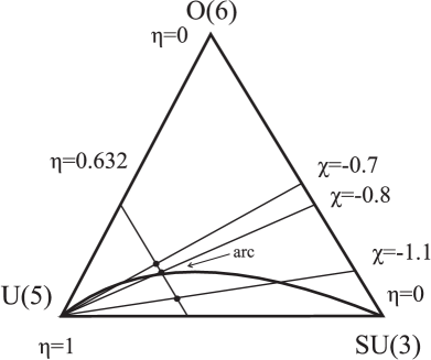
Figure 1: The IBM symmetry triangle and the points in the vicinity of the arc, where calculations were performed.

IV Numerical results

IV.1 Quantum chaotic dynamics of $0^{+}$ states

Measures of chaotic dynamics were calculated at four different points in the IBM symmetry triangle, as is shown in Fig. 1, namely on the SU(3) vertex, a point on the arc of regularity having parameters $(\eta,\chi)=(0.632,-0.803)$ and at two points with the same $\eta$ lying off the arc at $(\eta,\chi)=(0.632,-0.7)$ and $(\eta,\chi)=(0.632,-1.1)$. The value $\eta=0.632$ corresponds to $\zeta=0.7$ in a different parametrization Bon2 , and was chosen in order to be in accordance with the value used in Ref. Bon1 . The region of coexistence begins at $\eta=0.8$ . The points on the arc are given by the expression $\chi(\eta)=\frac{\sqrt{7}-1}{2}\eta-\frac{\sqrt{7}}{2}$, which was found by calculating the values of $\chi$ versus $\eta$, where $\sigma$ (a measure of classical chaos) is minimized Cejn2 .

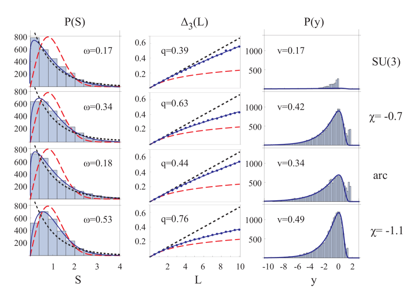
Figure 2: (color online) Results for the four points shown in Fig. 1, for $N_{B}=175$ and $J=0$ states, using the fluctuation measures $P(S)$ of Eq. (2) Brody and $\Delta_{3}(L)$ of Eq. (7) Dyson4 ; Mehta , and for $N_{B}=50$ and $J=0$ states, for the fluctuation measure $P(y)$ of Eq. (8) Levine ; Feingold . The black dotted line shows the regular limit, the red dashed line describes the chaotic limit, while the blue solid line is the fit to the distribution. It is evident from the values of $\omega$, $q$ and $\nu$, that the SU(3) vertex and the point on the arc are more regular compared to the other two points above and below the arc.

In order to have good statistics, $N_{B}=175$ was used for the fluctuation measures $P(S)$ and $\Delta_{3}(L)$, producing 2640 $0^{+}$ states. For the $P(y)$ fluctuation measure, $N_{B}=50$ was used, producing 54,756 possible transition strengths, $B(E0)$s, between the 234 $0^{+}$ states. The reason for selecting $N_{B}=50$ instead of $N_{B}=175$, was that in the latter case more than 6,000,000 possible transition intensities are produced between the 2640 $0^{+}$ states, which renders the calculation impossible to run in terms of time, while for $N_{B}=50$, the run time and the statistics are more than satisfactory. The allowed number of $B(E0)$s differs from point to point in the symmetry triangle of the IBM and this number gets larger, as the dynamics of the point get more chaotic. Figure 2 shows the results for the three statistical measures $P(S)$, $\Delta_{3}(L)$ and $P(y)$ applied on the three points illustrated in Fig. 1, accompanied by the results on the SU(3) vertex, a point with regular dynamics.

All three different measures of fluctuations show consistent results. The SU(3) vertex is the more regular point, followed by the point on the arc of regularity, which appears to also have regular behavior. Then come the points labelled by $\chi=-0.7$ and $\chi=-1.1$ which are indeed chaotic, with the $\chi=-0.7$ point being less chaotic than the $\chi=-1.1$ point. The fitting of the interpolating function of the last statistical measure, $P(y)$, on the SU(3) vertex is rather poor, which reflects the fact that the expression of Eq. (8) does not reduce to the regular case for any value of $\nu$.

Table 1: Spectra of $0^{+}$ states obtained from the Hamiltonian of Eq. (1) for $N_{B}=175$ and for the ($\eta$, $\chi$) parameter sets $(0,\frac{-\sqrt{7}}{2})$ [SU(3)], (0.632, $-0.803$) [arc], (0.632, $-0.7$) and (0.632, $-1.1$). In all cases the first $0^{+}$ state is set at zero and all other energies are normalized to the energy of the second $0^{+}$ state, i.e. to the energy of the first excited $0^{+}$ state. For each of the 8 intervals of 330 states each, into which the spectrum is divided, the energy of the highest state in the interval is shown.

state		SU(3)		arc		$\chi=-0.7$		$\chi=-1.1$
1		0		0		0		0
2		1		1		1		1
330		29.19		26.84		25.39		28.64
660		38.14		37.37		36.52		38.38
990		43.30		47.02		46.82		47.32
1320		46.49		56.16		56.57		55.74
1650		49.58		64.90		65.94		63.78
1980		52.74		73.42		75.00		71.54
2310		55.87		81.66		83.79		79.16
2640		59.00		92.74		94.28		91.17

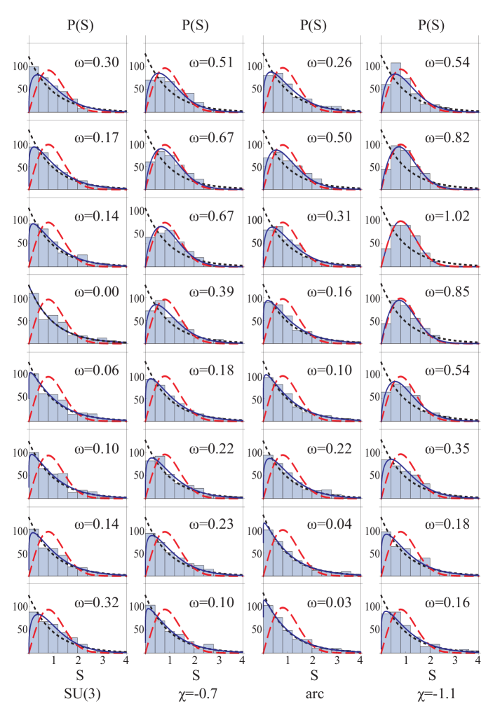
Figure 3: (color online) Results obtained for the nearest spacing distribution P(S) of Eq. (2) Brody for each of the cases shown in Fig. 1, for $N_{B}=175$ and, when the set of $J=0$ states is divided into 8 sets of 330 states each. The states 1-330 (labelled as interval 1 in Table 2) appear on the top, the states 2311-2640 (labelled as interval 8 in Table 2) appear at the bottom. The black dotted line shows the regular limit, the red dashed line describes the chaotic limit, while the blue solid line is the fit to the distribution.

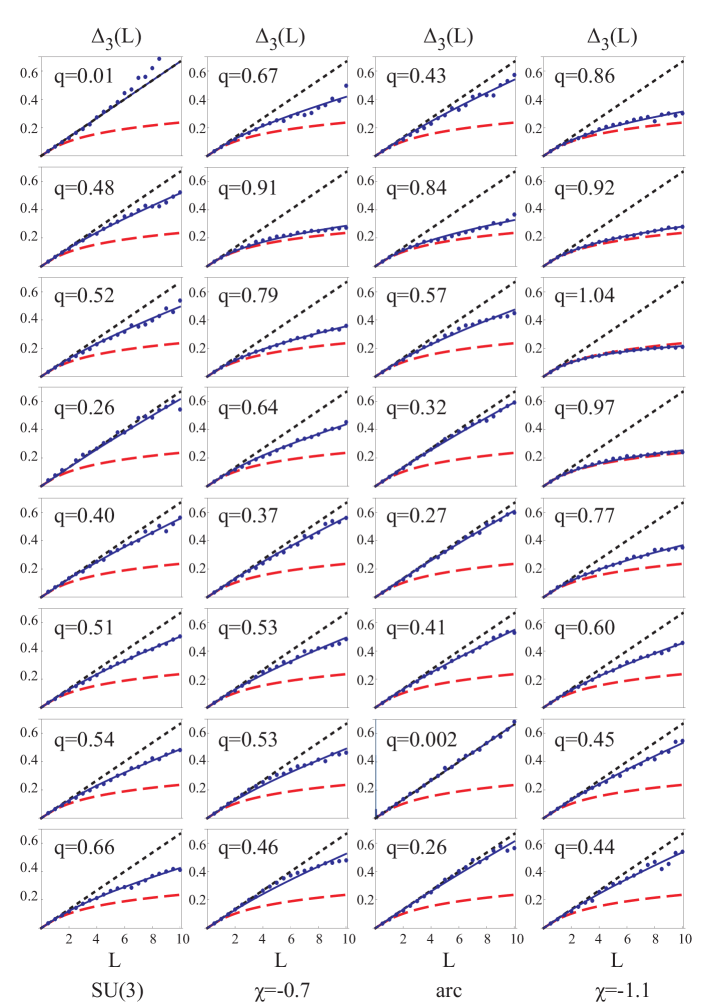
Figure 4: (color online) Results obtained for the spectral rigidity measure $\Delta_{3}^{q}(L)$ of Eq. (7) Dyson4 ; Mehta , for each of the cases shown in Fig. 1, for $N_{B}=175$ and, when the set of $J=0$ states is divided into 8 sets of 330 states each. The states 1-330 (labelled as interval 1 in Table 3) appear on the top, the states 2311-2640 (labelled as interval 8 in Table 3) appear at the bottom. The black dotted line shows the regular limit, the red dashed line describes the chaotic limit, while the blue solid line is the fit to the distribution.

Table 2: Numerical values of the parameter $\omega$ of the Brody distribution $P_{\omega}(S)$ of Eq. (2), for the 8 parts of each spectrum for $N_{B}=175$. The states 1-330 are labelled as interval 1, the states 2311-2640 are labelled as interval 8. The value of $\omega$ obtained from fitting the whole spectrum, coming from Fig. 2, is labelled by “total”.

interval		SU(3)		arc		$\chi=-0.7$		$\chi=-1.1$
P(S)		$\omega$		$\omega$		$\omega$		$\omega$
1		0.30		0.26		0.51		0.54
2		0.17		0.50		0.67		0.82
3		0.14		0.31		0.67		1.02
4		0.00		0.16		0.39		0.85
5		0.06		0.10		0.18		0.54
6		0.10		0.22		0.22		0.35
7		0.14		0.04		0.23		0.18
8		0.32		0.03		0.10		0.16
total		0.17		0.18		0.34		0.53

Table 3: Numerical values of the parameter $q$ of the $\Delta^{q}_{3}(L)$ distribution of Eq. (7) Dyson4 ; Mehta , for the 8 parts of each spectrum for $N_{B}=175$. The states 1-330 are labelled as interval 1, the states 2311-2640 are labelled as interval 8. The value of $q$ obtained from fitting the whole spectrum, coming from Fig. 2, is labelled by “total”.

interval		SU(3)		arc		$\chi=-0.7$		$\chi=-1.1$
$\Delta_{3}$(L)		$q$		$q$		$q$		$q$
1		0.01		0.43		0.67		0.86
2		0.48		0.84		0.91		0.92
3		0.52		0.57		0.79		1.04
4		0.26		0.32		0.64		0.97
5		0.40		0.27		0.37		0.77
6		0.51		0.41		0.53		0.60
7		0.54		0.002		0.53		0.45
8		0.66		0.26		0.46		0.44
total		0.39		0.44		0.63		0.76

IV.2 Chaos in $0^{+}$ states as a function of energy

The study of chaos as a function of energy, using the quantum spectrum, is for the first time possible, due to the large number of bosons used, which allows for good statistics. The spectrum of the produced states is divided into equal parts and each part is studied using the three statistical measures. For $N_{B}=175$, 2640 $0^{+}$ states are produced. The spectrum is divided into 8 parts of 330 states and each part is studied separately for its chaotic dynamics. The highest energy in each interval is shown in Table 1. In all cases the first $0^{+}$ state is set at zero energy, while all other energies are normalized to the energy of the second $0^{+}$ state, i.e. to the first excited $0^{+}$ state, thus rendering the parameter $c$ appearing in Eq. (1) irrelevant.

The spectra shown in Table 1 are the original ones, before any unfolding is applied to them. The division of the spectrum in parts of equal number of states, is the same as the division of the spectrum in parts having equal energy difference, due to the normalization of the spectrum which has led to neighboring energies differing on the average by 1. Figures 3 and 4 illustrate the results obtained for the nearest spacing distribution, P(S), and the spectral rigidity measure, $\Delta_{3}$(L), respectively. The first energy interval, i.e. the part with the states 1-330, appears at the top of the columns, while the last energy interval, the part with the states 2311-2640, appears at the bottom. The numerical results of $\omega$ and $q$ are displayed in Tables 2 and 3.

The degree of chaos is not uniform in energy. The low energy part of the spectrum (the first energy interval) is always less chaotic than the closest higher parts of the spectrum (the second and third energy intervals), where the motion becomes apparently chaotic. However, at higher energies chaos decreases significantly, the spectrum becoming almost regular at its highest part, even for the most chaotic point, $\chi=-1.1$. This behavior is common at all three points located at the vicinity of the arc. However, the SU(3) point, which is of course regular, seems not to follow the behavior of the others. Indeed, chaoticity falls in the middle part of the spectrum, and rises in the highest part, displaying exactly the opposite properties, although on the average the SU(3) point is less chaotic than the others, as indicated by the lowest values of $\omega$, $q$ associated with it in Fig. 2. Another observation is that the point on the arc is always less chaotic, in all energy intervals, compared to the points above and below the arc and that chaotic behavior is confined to fewer intervals at the arc or the SU(3) vertex.

These results are in accordance with several previous studies of both classical chaos and quantum chaos; for the latter non-statistical measures of chaos have been used so far. A few examples are listed here.

1) The energy dependence of regularity in the classical IBM has been studied for $\eta=0.5$ in Ref. Macek2 . Increased regularity has been found at low energies and again at high energies, while reduced regularity has been observed in between.

2) The energy dependence of regularity for a quantum IBM Hamiltonian has been studied, again for $\eta=0.5$, in Ref. Macek80 . Increased regularity has been observed in the AW arc region, both at low and at high energies. In this quantum study a visual method originally proposed by Peres Peres has been used, enabling a qualitative distinction between regular and chaotic motion.

3) The energy dependence of regularity in a quantum IBM Hamiltonian has been studied in a region corresponding to axially deformed ground states in Ref. Macek3 . Increased regularity, with strong occurence of SU(3)-like rotational bands, has been found at the AW arc at low energies and again at high energies, with reduced regularity occurring in between. Again the visual method of Peres Peres has been used.

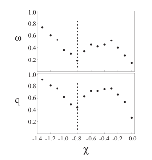
Figure 5: Results obtained for the quantum statistical parameters $\omega$ and $q$, for 14 different values of $\chi$ along the $\eta=0.632$ line of the triangle. The calculations were performed for $N_{B}=175$ and $J=0$.

IV.3 Chaos in $0^{+}$ states as a function of the parameter $\chi$

The results of the quantum statistical parameters, $\omega$ and $q$, as a function of the parameter $\chi$, determined at 14 different points along the $\eta=0.632$ line of the triangle, are seen in Figure 5. First, being on the SU(3)–U(5) line of the triangle ($(\eta,\chi)=(0.632,-1.32)$) chaotic behavior is displayed, which keeps diminishing as one reaches the arc of regularity ($(\eta,\chi)=(0.632,-0.803)$), where there is a minimum. Then, as one moves to larger values of $\chi$, chaoticity emerges again, but once more gives its place to regular behavior as one reaches the O(6)–U(5) line of the triangle ($(\eta,\chi)=(0.632,0)$), where the O(5) symmetry causes integrability Talmi .

The results for the $0^{+}$ states, are in complete agreement with the original work of Alhassid and Whelan, who found the existence of the arc of regularity using $N_{B}=25$ and $J\geq 2$ angular momentum. A strong peak on the arc of regularity has also been noticed in Ref. Macek2 , where the authors studied the dependence on $\chi$ at $\eta$=0.5 for the ratio of the number of regular trajectories to the total number of trajectories.

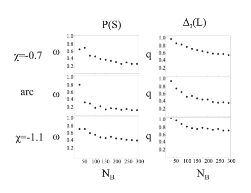
Figure 6: Results obtained for the quantum statistical parameters $\omega$ and $q$, for various values of $N_{B}$ at the three points in the vicinity of the arc of regularity.

IV.4 Chaos in $0^{+}$ states as a function of the number of bosons $N_{B}$

The results of the quantum statistical parameters, $\omega$ and $q$, as a function of the number of bosons $N_{B}$ are seen in Figure 6. In general, there is a drop of the values of the measured quantum statistical parameters $\omega$ and $q$ as $N_{B}$ increases. For small number of bosons (till about $N_{B}=100$) this drop is steep, while for larger $N_{B}$ (larger than $N_{B}=175$), the drop is very small and the quantum statistical parameters seem to have reached steady values. A reason for this steep drop, for small values of bosons, can be explained in terms of the total number of states for $J=0$, for different number of bosons, seen in Table 4, which affects the statistical results. For example, for $N_{B}=25$ there are only 65 states, which give barely sufficient statistics, for $N_{B}=50$ there are 234 states which give better statistics, while for $N_{B}=175$ there are 2640 states which give more validity to the statistical analysis of the eigenvalues. As the size of the system becomes larger, in the limit $N_{B}\rightarrow\infty$, $\omega$ and $q$ seem to approach fixed asymptotic values.

Table 4: Total number of states for $J=0$, for different number of bosons $N_{B}$.

$N_{B}$		Number of states		$N_{B}$		Number of states
25		65		175		2640
50		234		200		3434
75		507		225		4332
100		884		255		5334
125		1365		275		6440
150		1951		300		7651

Despite the drop of the values of the parameters, as a function of $N_{B}$, the point on the arc has the smallest values of $\omega$ and $q$, for all $N_{B}\geq 50$, compared to the other two points, $\chi=-0.7$ and $\chi=-1.1$, the point $\chi=-0.7$ being always less chaotic than $\chi=-1.1$ in the same $N_{B}$ region. The situation is different for $N_{B}=25$, where the value of $\omega$ is greater at the position corresponding to the arc of regularity, than at the neighboring points ($\chi=-0.7$ and $\chi=-1.1$). This comes as a surprise, since in their work, Alhassid and Whelan had used $N_{B}=25$ and $J=2$ or $J=10$ in order to locate the arc of regularity. Probably, the failure to locate the arc, using the fluctuation measure P(S), in our case, has to be attributed to the marginal badness of the statistics, since for $N_{B}=25$ and $J=0$ there are 65 states, while for $N_{B}=25$ and $J=2$ or $J=10$, there are 117 and 211 states respectively. However, as the number of bosons increases, the limiting values are quickly reached and the position of the arc of regularity becomes stable. One should recall at this point, that the nuclei found to lie close to the arc of regularity Jolie ; Amon have boson numbers close to $N_{B}=14$, therefore the location of the arc for these nuclei might be different from the one corresponding to the $N_{B}\to\infty$ limit.

Table 5: Numerical values of the parameter $\nu$ of the distribution $P_{\nu}(y)$ of Eq. (8) Levine ; Feingold , for the 8 parts of each spectrum for $N_{B}=50$. The states 1-30 are labelled as interval 1, the states 211-234 are labelled as interval 8. The value of $\nu$ obtained from fitting the whole spectrum, coming from Fig. 2, is labelled by “total”.

interval		arc		$\chi=-0.7$		$\chi=-1.1$
P(y)		$\nu$		$\nu$		$\nu$
1		0.40		0.62		0.44
2		0.48		0.81		0.84
3		0.39		0.60		0.87
4		0.32		0.49		0.77
5		0.29		0.35		0.54
6		0.23		0.26		0.37
7		0.21		0.21		0.30
8		0.21		0.27		0.22
total		0.34		0.42		0.49

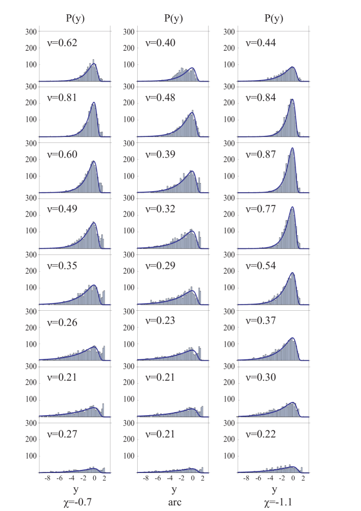
Figure 7: (color online) Results obtained for the statistical measure $P(y)$ of Eq. (8) Levine ; Feingold , for each of the cases shown in Fig. 1, for $N_{B}=50$ and, when the set of 234 $J=0$ states is divided into 7 sets of 30 states and one set of 24 states. The states 1-30 (labelled as interval 1 in Table 5) appear on the top, the states 211-234 (labelled as interval 8 in Table 5) appear at the bottom. The blue solid line is the fit to the distribution.

IV.5 Chaos in $B(E0)$ intensities as a function of energy

In the following subsections, a quantum chaotic study is carried out for the transition intensities between the $0^{+}$ states. The chaotic behavior of $B(E0)$ intensities as a function of energy is first presented. The 234 $0^{+}$ states occuring for $N_{B}=50$ were divided into 7 parts of 30 states each and one part of 24 states. For each interval of 30 $0^{+}$ states, the statistical measure $P(y)$ was applied to the $B(E0)$ intensities, produced by these 30 $0^{+}$ states. The results are displayed in Table 5 and in Figure 7. The first energy interval, i.e. the part with the states 1-30, appears at the top of the columns, while the last energy interval, the part with the states 211-234, appears at the bottom. The SU(3) point is missing from Table 5, for the following reason. As already mentioned, for points possessing some dynamical symmetry and thus characterized by regularity, as the SU(3) point, the interpolating function of Eq. (8) is poorly fitted, since the number of $B(E0)$ intensities occurring in this case is much smaller than the number of $B(E0)$ intensities obtained at other points, characterized by chaotic dynamics. In addition, these relatively few $B(E0)$ intensities are greatly dispersed. As a consequence, the study of chaos as a function of energy in the SU(3) limit, using $N_{B}=50$, was statistically impossible.

Again, the degree of chaos is not uniform in energy. The low energy part of the spectrum (the first energy interval) is always less chaotic than the next energy interval, where the motion becomes apparently chaotic. However, at higher energies chaos decreases significantly, the spectrum becoming almost regular at the highest part of the spectrum, even for the most chaotic point, $\chi=-1.1$. This behavior is common at all three points located in the vicinity of the arc. Again, the point on the arc displays less chaoticity, in all energy intervals, compared to the points above and below the arc and chaotic behavior is confined to fewer intervals at the arc. What is fascinating though, is that the study of quantum chaotic dynamics, both on the transition intensities and the spectrum of $0^{+}$ states, show consistency in the degree of chaos as a function of energy. In all cases, there is a jump in the degree of chaoticity as one passes the low part of the spectum, which is replaced by regularity as one gets at the upper part of the spectrum.

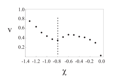
Figure 8: Results obtained for the quantum statistical parameter $\nu$, for 14 different values of $\chi$ along the $\eta=0.632$ line of the triangle. The calculations were performed for $N_{B}=50$ and $J=0$.

IV.6 Chaos in $B(E0)$ intensities as a function of the parameter $\chi$

The results of the quantum statistical parameter $\nu$, as a function of the parameter $\chi$, along the $\eta=0.632$ line of the triangle for $N_{B}=175$ are seen in Figure 8. For these calculations $N_{B}=50$ was used, which produced 54,756 possible $B(E0)$s between the 234 $0^{+}$ states.

The results show the same general behavior, as those of the quantum statistical parameters $\omega$ and $q$. There is a characteristic minimum of the curve, at $\chi=-0.8$, revealing the minimum chaoticity of the arc. Chaotic behavior is encountered at the regions below and above the arc of regularity, while at the O(6)–U(5) line of the triangle ($(\eta,\chi)=(0.632,0)$), regularity emerges again. The study of chaoticity of the $B(E0)$ intensities distribution gives results which are in complete agreement with the study of chaoticity of the $B(E2)$ intensities distribution of the original work of Alhassid and Whelan.

Table 6: Numerical values for $N_{B}=175$ of the parameter $\omega$ of the distribution $P_{\omega}(S)$ of Eq. (2) Brody , for the 7 points around the intersection (labelled as “on arc, on O(6)”) of the O(6) PDS line with the arc of regularity.

		$\chi$		$\eta$		$\omega$
below arc, on O(6)		-1.10		0.60		0.49
on arc, on O(6)		-0.88		0.54		0.16
on arc, right of O(6)		-0.98		0.41		0.23
on arc, left of O(6)		-0.80		0.63		0.18
above arc, on O(6)		-0.50		0.38		0.63
above arc, right of O(6)		-0.50		0.17		0.55
above arc, left of O(6)		-0.50		0.57		0.80

V Study of chaos on a line based on O(6) PDS

In addition to the notion of quasidynamical symmetry (QDS), i.e., the approximate persistence of a symmetry, in spite of strong symmetry breaking interactions Rowe1225 ; Rowe2325 ; Rowe745 ; Rowe756 ; Rowe759 , the notion of partial dynamical symmetry (PDS) has been introduced AL25 ; Lev77 ; LVI89 ; Lev2011 , including three different cases. In type I PDS part of the states possess all the dynamical symmetry, in type II PDS all the states possess part of the dynamical symmetry, while in type III part of the states possess part of the dynamical symmetry Lev2011 . The linkage between QDS and PDS has been only recently clarified, by proving that coherent mixing of one symmetry (QDS) can lead to partial conservation of a different, incompatible symmetry (PDS) Kremer .

In Ref. Kremer , by using a measure of $\sigma$ fluctuations in a state $\Psi$, called $\Delta\sigma_{\Psi}$, a valley of almost vanishing $\Delta\sigma_{g.s.}$ fluctuations has been found, i.e., a valley where the ground state wave functions have a high degree of purity with respect to the $\sigma$ quantum number of O(6), providing an example of an O(6) approximate PDS of type III. This line begins from the O(6) vertex and reaches the U(5)–SU(3) line of the triangle, intersecting, at a certain point, with the arc of regularity.

As a preliminary test, we applied the nearest neighbor spacing distribution, on $0^{+}$ states, for $N_{B}=175$ bosons, at various points on and around the O(6) PDS line, in order to see whether the O(6) PDS line induces regular dynamics to the $0^{+}$ states considered here. The results for the relevant parameter, $\omega$, are presented in Table 6. The only regular points are those located on the arc of regularity, including the intersection of the O(6) PDS line with the arc. Therefore, the O(6) PDS does not seem to induce regularity to the $0^{+}$ states considered here, a fact not unexpected, since the O(6) PDS regards the ground state band, while the present study focuses on all $0^{+}$ states, the two sets having only one state in common.

It is expected that in general PDS can lead to suppression of chaos, however this is expected to depend on the number of states exhibiting the PDS. In WAL71 a model Hamiltonian with an SU(3) PDS has been used, in order to examine whether there is suppression of chaos on the point of the PDS. Classical and quantum measures of chaos have been used for three different values of the angular momentum ($J=2,10,25$) and $N_{B}=25$. Minimum chaoticity has been found around the point where the SU(3) PDS was supposed to exist, but the minimum diverged slightly from this point for the two lowest values of angular momentum, while it was more pronounced and closer to this point for the larger value of angular momentum ($J=25$). The same behavior has been seen for the average SU(3) entropy of the eigenstates of the model Hamiltonian, which also showed a more pronounced and closer to the point of the SU(3) PDS minimum for $J=25$. This behavior has been explained in terms of the increase of the number of soluble states with increasing $J$. In contrast, in LW77 , where a large number of states had an SU(2) PDS, the classical and quantum measures of chaos showed a minimum exactly at the point where the SU(2) PDS was supposed to exist.

VI Conclusions

In this paper, we presented the application of statistical measures of chaos on the energy spectrum and the transition strengths of excited $0^{+}$ states, in the context of the interacting boson model and more precisely on a line connecting a point on the U(5)–SU(3) leg of the symmetry triangle with a point on the U(5)–O(6) leg. While the statistical measures of chaos reveal regularity on the U(5)–O(6) leg, due to the O(5) symmetry known Talmi to underlie this leg, the point on the U(5)–SU(3) leg seems to be the most chaotic point on this connection line. Besides the U(5)–O(6) leg, one more minimum is revealed on the transition line, located on the arc of regularity, which is in agreement with previous studies performed with smaller number of bosons and levels with angular momentum $J>2$.

Concerning the objectives posed at the end of the introduction, the following comments are in place.

1) The study of chaos as a function of energy gave some intriguing results. This study has already been performed using both classical Macek2 and quantum measures of chaos Macek80 ; Macek3 , but never using the fluctuation measures of the quantum spectrum or the transition intensities, due to the bad statistics imposed by the small number of bosons used. The degree of chaos differs as the energy changes. The results, both for the spectrum, as well as the transition intensities, show that the low energy part of the spectrum has always more regular dynamics compared to the immediately higher energy parts, which are almost completely chaotic. However, as the energy increases, chaoticity decreases and regularity prevails at the highest parts of the spectrum. This is the general behavior for points studied in the vicinity of the arc. However, the point on the arc is always more regular, compared to the other points, in all energy intervals, giving a confirmation for its regular character.

2) Quantum chaos also depends on the number of bosons used. As the number of bosons increases, the degree of chaos converges to a steady value. Beyond $N_{B}=50$, the relative chaoticity of different points is the same, for all numbers of bosons used in the context of this work. For example, chaoticity on the arc points is less than on the neighboring points, regardless of the number of bosons beyond $N_{B}=50$, giving for the arc a steady position in the symmetry triangle as a function of boson number beyond $N_{B}=50$. Below $N_{B}=50$, however, the location of the arc appears to be sensitive in $N_{B}$, this fact affecting the efforts of finding nuclei lying on or near the arc Jolie ; Amon , since the boson numbers corresponding to these nuclei are around $N_{B}=14$.

While the fluctuation measures of chaos reveal semiregularity on the arc, they cannot reveal the nature of the approximate symmetry underlying the Alhassid-Whelan arc of regularity, a question which has been addressed in several recent studies Macek80 ; Macek3 ; Bon1 ; Bon2 , but still remains open.

Recently, a line based on an O(6) PDS was found in the symmetry triangle, extending from the O(6) vertex to a point on the U(5)–SU(3) leg of the triangle, intersecting with the arc of regularity. Calculations of chaos around the intersection point show that the O(6) PDS does not contribute to the development of regular dynamics for the $0^{+}$ states, a reasonable result since the O(6) PDS under consideration regards only the ground state band of the nuclear spectrum.

The extension of the present study to states with non-zero angular momentum is desirable. In this case, attention should be paid to handling degeneracies in the spectrum Whe2 .

Study of the interplay of order and chaos has also been extended to the region of shape-phase transitions in the triangle. Shape phase transitions between different dynamical symmetries, as well as critical point symmeties appearing at the relevant transition points, have been an active field of investigation over the last decade JPG ; RMP . In the framework of the interacting boson model, in particular, a first order shape phase transition between spherical and deformed shapes is known to exist Feng , characterized by a phase coexistence region IZC . The appearance of degeneracies within the phase coexistence region PRL100 ; PRC80 , as well as the evolution of order and chaos across the first order transition ML84 ; LM714 ; LM2097 ; ML351 , are emerging fields of investigation.

References

- (1) F. Iachello and A. Arima, The Interacting Boson Model (Cambridge University Press, Cambridge, 1987).
- (2) R. F. Casten and E. A. McCutchan, Quantum phase transitions and structural evolution in nuclei, J. Phys. G: Nucl. Part. Phys. 34, R285 (2007).
- (3) P. Cejnar, J. Jolie, and R. F. Casten, Quantum phase transitions in the shapes of atomic nuclei, Rev. Mod. Phys. 82, 2155 (2010).
- (4) D. J. Rowe, Quasidynamical symmetry in an interacting boson model phase transition, Phys. Rev. Lett. 93, 122502 (2004).
- (5) D. J. Rowe, P. S. Turner, and G. Rosensteel, Scaling properties and asymptotic spectra of finite models of phase transitions as they approach macroscopic limits, Phys. Rev. Lett. 93, 232502 (2004).
- (6) D. J. Rowe, Phase transitions and quasidynamical symmetry in nuclear collective models: I. The U(5) to O(6) phase transition in the IBM, Nucl. Phys. A 745, 47 (2004).
- (7) P. S. Turner and D. J. Rowe, Phase transitions and quasidynamical symmetry in nuclear collective models. II. The spherical vibrator to gamma-soft rotor transition in an SO(5)-invariant Bohr model, Nucl. Phys. A 756, 333 (2005).
- (8) G. Rosensteel and D. J. Rowe, Phase transitions and quasi-dynamical symmetry in nuclear collective models, III. The U(5) to SU(3) phase transition in the IBM, Nucl. Phys. A 759, 92 (2005).
- (9) M. C. Gutzwiller, Chaos in Classical and Quantum Mechanics (Springer, Berlin, 1990).
- (10) F. Haake, Quantum Signatures of Chaos (Springer, Berlin, 2001).
- (11) Y. Alhassid and N. Whelan, Chaos in the low-lying collective states of even-even nuclei: Classical limit, Phys. Rev. C 43, 2637 (1991).
- (12) Y. Alhassid and N. Whelan, Chaotic properties of the Interacting Boson Model: A discovery of a new regular region, Phys. Rev. Lett. 67, 816 (1991).
- (13) Y. Alhassid and N. Whelan, Onset of chaos and its signature in the spectral autocorrelation function, Phys. Rev. Lett. 70, 572 (1993).
- (14) N. Whelan and Y. Alhassid, Chaotic properties of the interacting boson model, Nucl. Phys. A 556, 42 (1993).
- (15) N. Whelan, Ph.D. thesis, Yale University (1993).
- (16) J. Shu, Y. Ran, T. Ji, and Y.-X. Liu, Energy level statistics of the U(5) and O(6) symmetries in the interacting boson model, Phys. Rev. C 67, 044304 (2003).
- (17) R. F. Casten, Nuclear Structure from a Simple Perspective 2nd ed. (Oxford University Press, Oxford, 2000).
- (18) A. Leviatan, A. Novoselsky, and I. Talmi, O(5) symmetry in IBA-1 – The O(6)–U(5) transition region, Phys. Lett. B 172, 144 (1986).
- (19) P. Cejnar and J. Jolie, Dynamical-symmetry content of transitional IBM-1 hamiltonians, Phys. Lett. B 420, 241 (1998).
- (20) P. Cejnar and J. Jolie, Wave-function entropy and dynamical symmetry breaking in the interacting boson model, Phys. Rev. E 58, 387 (1998).
- (21) J. Jolie, R. F. Casten, P. Cejnar, S. Heinze, E. A. McCutchan, and N. V. Zamfir, Experimental confirmation of the Alhassid–Whelan arc of regularity, Phys. Rev. Lett. 93, 132501 (2004).
- (22) L. Amon and R. F. Casten, Extended locus of regular nuclei along the arc of regularity, Phys. Rev. C 75, 037301 (2007).
- (23) M. Macek, P. Stránský, P. Cejnar, S. Heinze, J. Jolie, and J. Dobes̆, Classical and quantum properties of the semiregular arc inside the Casten triangle, Phys. Rev. C 75, 064318 (2007).
- (24) M. Macek, J. Dobes̆, and P. Cejnar, Transition from -rigid to -soft dynamics in the interacting boson model: Quasicriticality and quasidynamical symmetry, Phys. Rev. C 80, 014319 (2009).
- (25) S. Heinze, P. Cejnar, J. Jolie, and M. Macek, Evolution of spectral properties along the O(6)-U(5) transition in the interacting boson model. I. Level dynamics, Phys. Rev. C 73, 014306 (2006).
- (26) M. Macek, J. Dobes̆, and P. Cejnar, Occurence of high-lying rotational bands in the interacting boson model, Phys. Rev. C 82, 014308 (2010).
- (27) M. Macek, J. Dobes̆, P. Stránský, and P. Cejnar, Regularity-induced separation of intrinsic and collective dynamics, Phys. Rev. Lett. 105, 072503 (2010).
- (28) D. Bonatsos, E. A. McCutchan, and R. F. Casten, SU(3) quasidynamical symmetry underlying the Alhassid–Whelan arc of regularity, Phys. Rev. Lett. 104, 022502 (2010).
- (29) D. Bonatsos, S. Karampagia, and R. F. Casten, Analytic derivation of an approximate SU(3) symmetry inside the symmetry triangle of the Interacting Boson Approximation model, Phys. Rev. C 83, 054313 (2011).
- (30) R. J. Casperson, Experimental and numerical analysis of mixed-symmetry states and large boson systems, Ph.D. thesis, Yale University (2010).
- (31) R. J. Casperson, IBAR: Interacting boson model calculations for large system sizes, Comp. Phys. Commun. 183, 1029 (2012).
- (32) Y. Alhassid and A. Novoselsky, Chaos in the low-lying collective states of even-even nuclei: Quantal fluctuations, Phys. Rev. C 45, 1677 (1992).
- (33) T. A. Brody, J. Flores, J. B. French, P. A. Mello, A. Pandey, and S. S. M. Wong, Random-matrix physics: spectrum and strength fluctuations, Rev. Mod. Phys. 53, 385 (1981).
- (34) F. J. Dyson and M. L. Mehta, Statistical theory of the energy levels of complex systems. IV, J. Math. Phys. 4, 701 (1963).
- (35) M. L. Mehta, Random Matrices, 2nd ed. (Academic Press, Boston 1991).
- (36) Y. Alhassid and R. D. Levine, Transition-strength fluctuations and the onset of chaotic motion, Phys. Rev. Lett. 57, 2879 (1986).
- (37) Y. Alhassid and M. Feingold, Statistical fluctuations of matrix elements in regular and chaotic systems, Phys. Rev. A 39, 374 (1989).
- (38) R. U. Haq, A. Pandey, and O. Bohigas, Fluctuation properties of nuclear energy levels: Do theory and experiment agree?, Phys. Rev. Lett. 48, 1086 (1982).
- (39) C. E. Porter and R. G. Thomas, Fluctuations of nuclear reaction widths, Phys. Rev. 104, 483 (1956).
- (40) A. Peres, New conserved quantities and test for regular spectra, Phys. Rev. Lett. 53, 1711 (1984).
- (41) Y. Alhassid and A. Leviatan, Partial dynamical symmetry, J. Phys. A: Math. Gen. 25, L1265 (1992).
- (42) A. Leviatan, Partial dynamical symmetry in deformed nuclei, Phys. Rev. Lett. 77, 818 (1996).
- (43) A. Leviatan and P. Van Isacker, Generalized partial dynamical symmetry in nuclei, Phys. Rev. Lett. 89, 222501 (2002).
- (44) A. Leviatan, Partial dynamical symmetries, Prog. Part. Nucl. Phys. 66, 93 (2011).
- (45) C. Kremer, J. Beller, A. Leviatan, N. Pietralla, G. Rainovski, R. Trippel, and P. Van Isacker, Linking partial and quasi dynamical symmetries in rotational nuclei, Phys. Rev. C 89, 041302(R) (2014).
- (46) N. Whelan, Y. Alhassid, and A. Leviatan, Partial dynamical symmetry and the suppression of chaos, Phys. Rev. Lett. 71, 2208 (1993).
- (47) A. Leviatan and N. D. Whelan, Partial dynamical symmetry and mixed dynamics, Phys. Rev. Lett. 77, 5202 (1996).
- (48) D. H. Feng, R. Gilmore, and S. R. Deans, Phase transitions and the geometric properties of the interacting boson model, Phys. Rev. C 23, 1254 (1981).
- (49) F. Iachello, N. V. Zamfir, and R. F. Casten, Phase coexistence in transitional nuclei and the interacting-boson model, Phys. Rev. Lett. 81, 1191 (1998).
- (50) D. Bonatsos, E. A. McCutchan, R. F. Casten, and R. J. Casperson, Simple, empirical order parameter for a first order quantum phase transition in atomic nuclei, Phys. Rev. Lett. 100, 142501 (2008).
- (51) D. Bonatsos, E. A. McCutchan, R. F. Casten, R. J. Casperson, V. Werner, and E. Williams, Regularities and symmetries of subsets of collective 0+ states, Phys. Rev. C 80, 034311 (2009).
- (52) M. Macek and A. Leviatan, Regularity and chaos at critical points of first-order quantum phase transitions, Phys. Rev. C 84, 041302(R) (2011).
- (53) A. Leviatan and M. Macek, Evolution of order and chaos across a first-order quantum phase transition, Phys. Lett. B 714, 110 (2012).
- (54) A. Leviatan and M. Macek, Order, chaos and quasi symmetries in a first-order quantum phase transition, J. Phys. Conf. Ser. 538, 012012 (2014).
- (55) M. Macek and A. Leviatan, First-order quantum phase transitions: test ground for emergent chaoticity, regularity and persisting symmetries, Ann. Phys. (N.Y.) 351, 302 (2014).