Two step mechanism for Moreton wave excitations in a blast-wave scenario
A case study: the December 06, 2006 event

Abstract

We examine the capability of a blast-wave scenario -associated to a coronal flare or to the expansion of CME flanks- to reproduce a chromospheric Moreton phenomenon. We also simulate the Moreton event of December 06, 2006 considering both the corona and the chromosphere. To obtain a sufficiently strong coronal shock -able to generate a detectable chromospheric Moreton wave- a relatively low magnetic field intensity is required, in comparison with the active region values. Employing reasonable coronal constraints, we show that a flare ignited blast-wave or the expansion of the CME flanks emulated as an instantaneous or a temporal piston model, respectively, are capable to reproduce the observations.

1 Introduction

Moreton waves, a class of large-scale chromospheric disturbances, are detected in emission in the center and blue wing of the H$\alpha$ spectral line, whereas they appear in absorption in the red wing, which is interpreted as a compression and subsequent relaxation of the chromosphere (Uchida, 1968; Vršnak et al., 2002a). They propagate forming an arc-shaped imprint out of the flare sites, constrained in a certain angular span at distances as long as $500$ Mm, with radial velocities ranging from $500$ km s^-1 to $2000$ km s^-1 (Moreton, 1960; Moreton & Ramsey, 1960; Athay & Moreton, 1961).

Although Moreton waves are typically observed in chromospheric spectral lines (H$\alpha$), there is consensus that they are of coronal origin since their high speeds are much larger than the characteristic speeds in the chromosphere. Uchida (1968) and Uchida et al. (1973) proposed a blast-wave scenario where Moreton waves are interpreted as fast-mode MHD shocks expanding in the corona, which produce a chromospheric disturbance due to the shock “sweeping” over the chromospheric surface. Further reinforcements of this freely propagating large amplitude “single wave” scenario are the deceleration of the wavefronts, the elongation of the perturbations, and the decreasing amplitude of the disturbances (Warmuth et al., 2001, 2004a). Commonly, the sudden oscillation and winking of distant filaments are associated to the passage of the Moreton disturbances (Gilbert et al., 2008; Francile et al., 2013), suggesting that Moreton waves are not always visible at chromospheric levels.

At other wavelengths, similar transient wave-like features were reported, e.g., for the Helium I 10830Å line, soft-X rays and microwaves (Gilbert & Holzer, 2004; Warmuth et al., 2005; Vršnak et al., 2002a; Aurass et al., 2002; Warmuth et al., 2004a). In the extreme ultraviolet (EUV), global propagating disturbances were firstly observed by the EUV Imaging Telescope (EIT) aboard the Solar and Heliospheric Observatory (SOHO) (Thompson et al., 1998; Delaboudinière et al., 1995) and, some authors argue that EIT waves are the coronal counterpart of Moreton waves as they are co-spatial (Warmuth et al., 2001, 2004b). Since then, they have been extensively studied giving rise to a controversy regarding the wave or non-wave nature of these “EIT” (also EUV) disturbances (see White et al. (2014) and references therein). Recent observations give support to the coexistence of a bimodality character of these EIT disturbances: both the wave (fast mode) and the non-wave physical mechanisms can be at work in the same event, although not always detected with the current instrumentation (Zhukov & Auchère, 2004). This would lead to the possibility of multiple driven mechanisms, as proposed by Gilbert & Holzer (2004) and Zhukov (2011). Also, while some authors find that the EIT and Moreton waves have approximately the same speed, others claim that EIT waves are slower than Moreton waves by a factor of two to three (Chen et al., 2002, 2005; Zhang et al., 2011).

Solar flares and coronal mass ejections (CMEs) are atmospheric explosive phenomena capable to produce large-amplitude coronal disturbances and shock waves leading to the formation of a Moreton wave. The most straightforward model to give account of the shock formation is a 3D piston mechanism. The flare ignited blast-wave model (or simple 3D shock model) assumes that a temporal piston mechanism is caused by the energy release of a flare-volume expansion that produces an explosion-like process driven by a pressure pulse (Vršnak & Cliver, 2008). On the other hand, the CME-driven shock model proposes that the expansion of a CME, together with the rise of a corresponding flux rope, produces a combination of a piston-shock and a bow-shock, which generates the large-scale shock wave (Chen & Shibata, 2000; Chen et al., 2002). Temmer et al. (2009) stated that the observation of Moreton waves can only be reproduced by applying a strong and impulsive acceleration for the source region expansion acting in a temporal piston mechanism scenario. They proposed that the expansion of the flaring region or the lateral expansion of the CME flanks is more likely the driver of the Moreton wave that the upward moving CME front.

The flare-CME controversy also extends to the origin of type II radio burst that are usually observed close in time and distance to the shock source. They are interpreted to be the emission, at the local plasma frequency, of shock accelerated electrons producing Langmuir waves (Knock et al., 2001). While there is a consensus that the emission in the decameter or longer wavelength range is associated with CMEs, metric wavelengths can be due either to flare or CME ignited shocks (see e.g. Vršnak & Cliver (2008)). Recent papers show evidence of type II radio burst associated with a flare without a CME companion (Magdalenić et al., 2012; Su et al., 2015).

Thus, two different views on the origin of large-scale coronal shock waves arise, one favoring CMEs and the other preferring flares. In favor of the flare model it is argued that the required Moreton wave acceleration is larger or more impulsive than the usually observed values for CMEs. However, the large discrepancy between the great number of registered flare events and the relatively rare occurrence of observable coronal shocks (Cliver et al., 1999) suggests that, in addition to the flare explosion, another mechanism could be necessary to produce large-scale waves, or that a very special condition must be accomplished for the shock formation. In fact, following an analysis of orders of magnitude, Vršnak & Cliver (2008) showed that relatively high values of the plasma parameter (plasma-to-magnetic pressure ratio) $\beta\approx 0.1-0.01$ are required to ignite a coronal shock wave (at least two orders of magnitude larger than in an active region where $\beta\approx 0.0001$). This could explain the rarity of Moreton waves, as they should be triggered at the peripheries of active regions where the magnetic field is decaying. An alternative reasoning of this argument is given in the Appendix.

Several numerical simulations have been carried out to try to explain large-scale wave formations in the solar atmosphere. 3D MHD numerical simulations were performed considering a solar flare-induced pressure pulse (Wu et al., 2001), and although the main characteristics of the observed EIT waves were reproduced, the plasma parameter used $\beta\sim 1$, was too large. The CME scenario has also been simulated. In many cases an ad-hoc force is used to model the eruptive flux rope that triggers the expansion of the CME flanks and drives the shock (Chen et al., 2002, 2005; Mei et al., 2012). The simulated shock sweeps the chromosphere forming the Moreton wave, where a slower wave (identified as the EIT wave) propagates outwards. Whether the resulting weak coronal CME shock can produce a detectable chromospheric Moreton wave is part of the controversy since to do so the expansion has to be accelerated to velocities which are rare in CMEs.

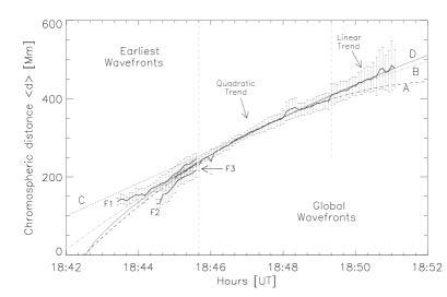
Figure 1: Solid line: $2$D averaged chromospheric distance $\langle d\rangle$ from $Q_{0}$ with a $1$ sigma dispersion value. Earliest wavefronts $F_{1},F_{2},F_{3}$ before $t$=$18$:$45$:$40\ \mathrm{UT}.$ $A:$ partial quadratic fit. $B:$ Total quadratic fit. $C:$ Partial linear fit. $D:$ Power-law fit (taken from Francile et al. (2013)).

In Francile et al. (2013) we studied a Moreton wave detected on December 06, 2006 with the H$\alpha$ Solar Telescope from Argentina (HASTA) in the H$\alpha$ line $656.3$ nm. We determined the kinematics of the whole complex process through a 2D reconstruction of the HASTA and corresponding TRACE observations (Transition Region And Coronal Explorer, Handy et al. (1999)). In Figure 1 we synthesized the observational results of the chromospheric distances traveled by the Moreton wave as a 2D planar projection, perpendicular to the line of sight. The evolution of the Moreton wave lead to the activation of two distant filaments. We also noted three initial irregular wavefronts that can be attributed to local inhomogeneities of the coronal medium crossed by the disturbance. We used different fits to describe the kinematics of the event. Curve $D$ is a power-law fit on the complete set of wavefront data. The resulting initial acceleration of the curve is $a_{0}\approx-30.2$ km s^-2 (starting with an initial speed of $s_{0}\geq 2121$ km s^-1 at $t=18:42:30$ UT). A partial quadratic fit trend $A$ associated with an acceleration of $a\geq-2.4$ km s^-2 was also used to adjust the data ranging within $[18:45:40-18:49:02]$ UT with an initial speed of $s_{0}\geq 1463$ km s^-1 (extrapolated at $18:42:28$ UT). The quadratic acceleration value and the initial speed are higher than those obtained by other authors for the same event (Balasubramaniam et al., 2010). The partial linear fit trend $A$ of the figure corresponds to a free wave speed of $\approx 700$ km s^-1. We concluded that the Moreton wave event observed on December 6, 2006 can be interpreted as a coronal fast-shock wave of a blast type originated by a single flare source during a CME ejection. However, its onset time is concurrent with the peak of the Lorentz force applied to the photosphere measured by Balasubramaniam et al. (2010) showing an overlap with the flare explosive phase and other minor scale events. This argument favors the hypothesis that the phenomenon can be described as the chromospheric imprint of a fast coronal shock triggered from a single source in association with a CME.

In this work, to reproduce the observational description in Francile et al. (2013), we present a 2D numerical simulation of the December 6, 2006 Moreton wave. The initial configuration is a simplified 2D blast-wave scenario able to trigger a real, freely propagating MHD wave without considering the magnetic field restructuring of a CME. The blast-wave, acting as a piston mechanism is emulated by both, an instantaneous pressure pulse and other one that extends over a short time which could also resemble the action of the flank expansion of a CME. The aim is to discuss whether the instantaneous and temporal piston models are capable to reproduce the main characteristics of the observations. We here use the word ‘instantaneous’ to distinguish a pulse used only as the initial condition, from another one where the pulse is imposed for a given lapse of time of the run, named ‘temporal pulse’.

The Model

The 2D ideal MHD equations for a completely ionized hydrogen plasma, with $\gamma=5/3$, ($\gamma$ the ratio of specific heats) were implemented to study Moreton waves in the frame of the blast-wave scenario. We first use a pressure pulse to simulate the flare-volume expansion (instantaneous piston mechanism) that causes the blast-wave propagating fast-mode shock which sweeps the chromosphere (Uchida, 1968; Uchida et al., 1973). The pressure pulse emulates the result of different complex processes that can trigger the flare activity and impulsively heat the active region (AR) (Wu et al., 2001; Guo et al., 2013; Onofri et al., 2004). The ideal MHD equations, in conservative form, result:

$$\frac{\partial\rho}{\partial t}+\mathbf{\nabla}\cdot(\rho\mathbf{v})=0$$ (1)

$$\frac{\partial\rho\mathbf{v}}{\partial t}+\mathbf{\nabla}\cdot\left(\rho\mathbf{v}\mathbf{v}-\frac{\mathbf{B}\mathbf{B}}{4\pi}+\mathbf{I}\left(p+\frac{B^{2}}{8\pi}\right)\right)=0$$ (2)

$$\frac{\partial\varepsilon}{\partial t}+\mathbf{\nabla}\cdot\left(\mathbf{v}\left(\varepsilon+p+\frac{B^{2}}{8\pi}\right)\right)=0\ ,$$ (3)

where $\rho$ indicates the density, $\mathbf{v}$ the velocity, $\mathbf{B}$ the magnetic field, $p$ is the pressure and $\varepsilon$ the energy density given by

$$\varepsilon=\frac{p}{\gamma-1}+\frac{1}{2}\rho v^{2}.$$ (4)

As we are interested in low coronal phenomena (flare ignition scenario) and considering typical large values of the coronal pressure scale height, $\approx 100$ Mm, we neglect the gravity term in the equations.

Our aim is to describe the effect of the coronal wave over the transition region and the upper chromosphere. Thus, the chromosphere is modeled as a thin simple layer where the pressure is constant and the temperature and density abruptly change at the transition region. The height of the region is arbitrarily assumed as $5$ Mm, approximately twice the height of the H_α line core formation (Leenaarts et al., 2012). We assume that the excess of the H_α core emission generated by the compression of the coronal shock is only due to the action of the upper chromosphere (observationally quantified by techniques of running differences). Following Leenaarts et al. (2012) the emission of the H_α line core is strongly correlated with the mass density, and is only weekly modulated by the temperature and the velocity. Thus, the density traces the variations caused by the magnetic field, the waves and shock waves. Also, as stated by Leenaarts et al. (2007) this region can be considered as optically thin outside dynamic magnetic structures as fibrilles.

The shock wave characteristics are given by the coronal properties. Since the ratio of the coronal gas pressure to the magnetic pressure is $\beta\sim c_{s}^{2}/v_{A}^{2}\ll 1$ ($c_{s}$ the acoustic speed and $v_{A}$ the Alfvén speed) the velocity of the coronal fast magnetosonic shock caused by the flare will mainly depend on the magnetic field through the Alfvén speed. Also, as stated by the Rankine-Hugoniot conditions, the observational amplitude of the emitted wave is directly related to the pressure (or density) increase through the shock, i.e., the compression ratio (Vršnak et al., 2002b; Vršnak & Cliver, 2008). The question is, again, if the pressure gradient can produce a sufficiently strong shock wave in the ambient corona able to generate a detectable chromospheric Moreton wave. Although the AR pressure can increase several times according with the admissible values of temperature and density (see e.g. Aschwanden (2005)), limitations arise because whereas a sufficiently strong magnetic field is required to reach the correct velocity of the magnetosonic shock, the shock intensity rapidly decays with increasing magnetic fields (see the Appendix). Thus, to obtain a sufficiently large perturbation a larger pressure pulse is needed. However, there is an upper limit for the temperature and density values. A typical AR temperature threshold should be as large as $40\times 10^{6}$ K, (Aschwanden, 2005). An alternative would be to investigate the effect of a temporal pressure pulse, allowing a lower pressure pulse, though acting along time. With the aim of reproducing the observational HASTA results and considering this constraint, we analyze the influence of the magnetic field in the formation of large scale solar waves for a uniform magnetic field assumption.

Numerical code and initial conditions

For the numerical simulations we use the FLASH code developed at the Center for Astrophysical Thermonuclear Flashes (Flash Center) of the University of Chicago (Fryxell et al., 2000). This code, currently in its fourth version, can be used to solve the compressible magnetohydrodynamics equations with adaptive mesh refinement (AMR) capabilities. We choose for our simulations the “Unsplit Staggered Mesh” scheme (Lee et al., 2009) available in FLASH, which uses a high resolution finite volume method with a directionally unsplit data reconstruction and the constraint transport method (CT) to enforce the $\nabla\cdot\mathbf{B}=0$ condition. The Riemann problems of the computational interfaces are calculated by a Roe-type solver.

A cartesian 2D grid with a discretization of $20\times 10$ cells is used with $8$ levels of refinement. The refinement criterion takes into account the variations of the density, pressure and magnetic field (the maximum refinement corresponds to a cell of $0.39$ Mm). The physical domain is set to $(1000,500)$ Mm and consists of two regions that model the solar atmosphere: the chromosphere formed by a small region above the solar surface, and the corona.

Initially the atmosphere is in total equilibrium with a uniform ambient magnetic field (open-field assumption). Thus, the plasma pressure is constant in the initial equilibrium configuration. On the other hand, although in this flare-ignited scenario the interest is focused in describing low coronal features, the physical domain was extended in the vertical direction to avoid possible spurious results generated by the interaction between the shock and the upper boundary. We choose typical values of temperature and number density at the coronal base, $T_{\rm u}=1.6\times 10^{6}$ K and $n_{\rm u}=1.2\times 10^{8}$ cm^-3 (Wu et al., 2001). The number density in the chromosphere is obtained considering an initial temperature of $T_{\rm d}=1\times 10^{4}$ K, and the same plasma pressure as in the corona. As mentioned, the pressure pulse intensity is limited by the maximum admissible temperature and density, which can increase up to $T\approx 40\times 10^{6}$ K and $n\approx 10^{11}$ cm^-3 e.g., if we consider a flaring loop (Aschwanden, 2005).

Firstly, the pressure pulse is instantaneously triggered at $t=0$ s. The number density is mantained constant and the temperature is determined by the applied pressure pulse variation, but, if for a given pressure increment the maximum temperature is exceeded, the density is increased to maintain the temperature below the threshold. The size of the pressure pulse is fix to $10$ Mm, in accordance with typical flare kernel sizes (Vršnak & Cliver, 2008). The distance between the pressure pulse location and the chromospheric surface is set to adjust the space-time interval between the flare event and the beginning of the Moreton wave reported by the observations. We assume that the flare occurs near the boundary of the AR where the magnetic field has already decay and we study the propagation of the perturbation from the boundary of the AR across the quiet corona where the magnetic field is assumed uniform. The magnetic field is varied within $\sim[1-10]$ G to adjust the phenomenological values of Figure 1. Secondly, the procedure is repeated using a temporal pressure pulse, i.e., a pulse applied during a lapse of time, to be determined in order to fit the observations. This case could represent the action of the flank expansion of a CME as suggested by Temmer et al. (2009).

Figure 2 shows the setup of the physical model, with the upper coronal region and the downward chromospheric one. We use free-flow conditions (zero gradient values) for the upper and lateral boundaries and a reflecting condition for the lower boundary to model the denser solar surface values.

Figure 2: 2D simulation scheme. Corona: $T_{\rm u}=1.6\times 10^{6}$ K,   $n_{\rm u}=1.2\times 10^{8}$ cm^-3,   $p_{\rm u}=0.0265$ dyn cm^-2. Chromosphere: $T_{\rm d}=10^{4}$ K, $p_{\rm d}=p_{\rm u}$,   $n_{\rm d}=1.92\times 10^{10}$ cm^-3. The chromospheric height is $5$ Mm and $h=35$ Mm is the distance of the pressure pulse ($\Delta p$) from the interface corona-chromosphere.

Results and Discussion

Kinematics: a two step mechanism

To give account of the two step mechanism is essential to simulate the chromosphere as a dense thin layer where the coronal perturbation penetrates and rebounds. To understand how these two mechanisms act we analyze Figure 3. The figure shows a zoom, at $t=300$ s, of the numerical simulation domain where a coronal disturbance is triggered by a pressure pulse $\Delta p/p=100$ times larger than the ambient pressure, located at a height $h=35$ Mm with a uniform magnetic field $B_{0}=1$ G. There are two main effects of the shock front over the interface corona-chromosphere: (first step) an intense compression of the chromosphere acting persistently in the vertical direction (note the vertical discontinuity in Figure 3a-d at $x\sim 18$ Mm), which is firstly initiated remaining quasi-stationary, and, (second step) a circular shaped shock or chromospheric disturbance, appearing delayed with respect to the initial compression that travels in the corona and “sweeps” the chromosphere. We note that behind the leading shock wave ($x\sim 120$ Mm at a coronal height of $h\sim 35$ Mm) there is a complex pattern of interacting waves. This nonlinear interaction is able to weaken the leading shock and consequently the Moreton wave (see a simpler study of the nonlinear interaction, where the combined wave front is plane in e.g., Fernández et al. (2009), Costa et al. (2009) and Cécere et al. (2012)).

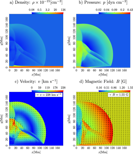
Figure 3: Coronal fast MHD shock at $t=300$ s with $B=1$ G. Panel a) shows the density; panel b) shows the pressure; panel c) shows the velocity and panel d) shows the magnetic field.

Figure 4 shows a temporal scheme of the second step procedure: the initiation of the traveling chromospheric disturbance. At $(x_{C0},t_{0})$ the blast coronal wave is triggered. The point $(x_{I1},t_{1})$ shows the space-time location where the blast arises to the interface corona-chromosphere (point $(x_{C1},t_{1})$ is its corresponding coronal counterpart). For each $j$, $(x_{Cj},t_{j})$ and $(x_{Ij},t_{j})$ are a coronal and a chromospheric space-time point that belong to the same wavefront. Due to the geometrical characteristic of the scenario, while the wavefront travels from $t_{1}$ to $t_{2}$ a distance $d_{C1}=x_{C2}-x_{C1}$ in the corona, the corresponding intersection, lying in the interface corona-chromosphere, travels a larger distance $d_{I1}=x_{I2}-x_{I1}$. Note that, while for earlier times $d_{Cj}<d_{Ij}$, for longer ones $d_{Cj}\sim d_{Ij}$. Therefore, the initial coronal wave speed is slower than the chromospheric one and they become increasingly similar for larger times. This corresponds to a virtual deceleration given by the variation of the speed of a virtual point determined by the intersection between the chromosphere and the wavefront. This could give account of the strong initial deceleration of Moreton waves, also explaining why some authors find that these waves are faster than EIT waves (Zhang et al., 2011). Later, when the wavefront is capable to sweep a detectable amount of chromospheric material, a real free wave that lags with respect to its coronal counterpart is observed.

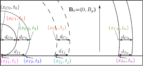
Figure 4: Scheme of the two step mechanism. The flare originates at the corona at $(x_{C0}=0,t_{0})$. The wavefront arrives to the corona-chromosphere interface at $(x_{I1}=0,t_{1})$, when the coronal wavefront has traveled a distance $d_{C0}$ from the origin. At $t_{2}$, the coronal wavefront has traveled a distance $d_{C1}$ from $x_{C1}$ while the chromospheric front has traveled a distance $d_{I1}>d_{C1}$. Thus, the chromospheric wavefront speed is larger than the coronal one, $d_{I1}/(t_{2}-t_{1})=(x_{I2}-x_{I1})/(t_{2}-t_{1})>d_{C1}/(t_{2}-t_{1})=(x_{C2}-x_{C1})/(t_{2}-t_{1})$. For later times, the coronal wavefront speed and the chromospheric one become increasingly similar, $d_{Ij}/(t_{j+1}-t_{j})\simeq d_{Cj}/(t_{j+1}-t_{j})$. The chromospheric wavefront lags with respect to the coronal one.

In Figure 5a-b we display two density profile slices: Figure 5a at the coronal level ($h=35$ Mm above the interface corona-chromosphere) and Figure 5b located in the chromospheric upper layer ($100$ km below the interface corona-chromosphere), at $t=300$ s. The initial background magnetic field used is $B_{0}=3$ G and the triggering pressure pulse is $\Delta p/p=100$. In the coronal case an evident shock is appreciated ($200$ Mm $\leq x\leq 230$ Mm), with a sharp density enhancement followed by a rarefaction. This fall of the density behind the shock could be an alternative explanation for the dimming of EUV observations (see also Figure 3), which are usually associated with the eruptive volume expansion of CMEs (Chen et al., 2002). At the chromospheric level, we note a deep persistent vertical compression (first step: $x\leq 170$ Mm) that pushes down the interface chromosphere-corona, and a traveling front of density enhancement (second step: $170$ Mm $\leq x\leq 220$ Mm) more diffuse and less intense than the coronal one. Taking into account that the H$\alpha$ opacity in the upper chromosphere is mainly sensitive to the mass density (the upper chromosphere can be considered as an optically thin media) and only weakly sensitive to the temperature (Leenaarts et al., 2012), we assume that this density profile gives account of the Moreton disturbance. As in White et al. (2014) (see Figure 3 of their paper), we note that there is a lag between the chromospheric perturbation and the coronal signal. In this case, at $t=300$ s, the chromospheric perturbation lags $\approx 30$ Mm behind the coronal signal. This is reinforced by the observation of the early activation of two distant filaments with respect to the chromospheric Moreton wave evolution, even in regions where it is no longer detectable, (Francile et al., 2013). If we consider different times (not shown in the figure), after the initial transitory, we find that the two signals travel with similar speeds and trajectories.

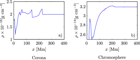
Figure 5: Density profiles in the solar atmosphere for $t=300$ s and $B_{0}=3$ G, $\Delta p/p=100$. a) corona; b) chromosphere.

In Figure 6 we present the distance traveled by a chromospheric disturbance as a function of time for different uniform magnetic field values. A typical Moreton wave kinematics is obtained (see Table 1), i.e., a strong initial deceleration, that gradually diminishes which is larger for larger magnetosonic velocities (stronger magnetic fields). This characteristic behavior is in agreement with the results in Francile et al. (2013) where we detected a Moreton wave with an initial deceleration of $\sim-30$ km s^-1 that diminishes to $\sim-2.4$ km s^-1 in an almost quadratic trend before it finishes in a linear one. The $t$ values of the table are the first detection times of the chromospheric traveling perturbation. The initial time interval with a lack of data is the time that takes the vertical coronal front, traveling with a fast magnetosonic shock speed, to arrive to the corona-chromosphere interface. However, the Moreton wave detection requires that the coronal perturbation compresses the chromosphere beyond a certain threshold, which was not taken into account to perform the figure. As in the observations, the simulations show that the chromospheric wave speed gradually becomes slower until the shock evolves to an ordinary fast magnetosonic disturbance (the linear region of the curves in Figure 1 and Figure 6) (Warmuth et al., 2004b).

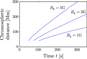
Figure 6: Distances traveled by the Moreton wave as a function of time, for different values of the magnetic field. $\Delta p/p=100$.

$B_{0}$[G]	$v$[km s${}^{-1}]$	$a$[km s${}^{-2}]$	$t$[s]
$1$	$594$	$-7$	$100$
$3$	$1065$	$-13$	$74$
$5$	$1876$	$-35$	$46$

Table 1: Simulated models: $B_{0}$ is the initial background magnetic field, $v$ is the velocity in $x$ direction, $a$ is the acceleration and $t$ is the time of the first disturbance detection.

In Francile et al. (2013) a compression ratio of $\Delta\rho\gtrsim 0.08\times\rho_{0}$ was required to obtain a detectable chromospheric perturbation which leads to a certain distance between the radiant point (the probable location of the single wave source projected into the chromosphere) and the place where the Moreton wave is initially visible. Figure 7 shows the temporal average of both, a) the compression ratio ($\Delta\rho/\rho_{0}$) and b) the front velocity of the coronal shock as a function of the pressure pulse strength for different magnetic field values. As mentioned before, the velocity and the compression ratio are mainly defined by the magnetic field intensity: strong fields ($\beta\ll 1$) cause large shock speeds but small compression ratios. Moreover, the coronal shock speed is almost constant while varying the pressure pulse, specially for large values of the magnetic field, e.g., an increase of three orders of magnitude in $\Delta p/p$ implies an enhancement of the shock speed of $\sim 130\%$ for a magnetic field of $B_{0}=1$ G and, of $\sim 10\%$ for $B_{0}=5$ G. Note that to obtain a linear shock speed trend of about $700$ km s^-1 (as in Figure 1, which is also the typical averaged Moreton wave speed (Zhang et al., 2011)), we need a magnetic field $\geq 3$ G, but due to the rapid decrease of the compression ratio with increasing magnetic fields, it could be possible that the corresponding coronal compression ratio is insufficient to produce a detectable chromospheric compression with the HASTA instruments (a compression ratio of $8\%$ is required), even for the larger allowed values of the pressure pulse. This would be in accordance with the fact that, when detected, the Moreton events are generally associated with intense flares with an impulsive phase, usually leading to type II radio burst (Uchida, 1968).

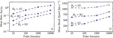
Figure 7: Coronal mean compression ratio a) and velocity b) for the shock wave considering different values of the magnetic field strength and the pressure pulse intensity.

To analyze if the coronal shock is capable to produce a detectable Moreton wave we study the chromospheric density profiles. We plot the density values at the $y$ coordinate positions lying in a slice (along the $x$ coordinate) located just below the unperturbed upper chromospheric layer as depicted in Figure 8. Time $t=0$ s (Figure 8a) corresponds to the flare ignition and subsequent times indicate the evolution of the Moreton wave (see the chromospheric density profiles given in Figure 8b-d, for $t=200,400,600$ s, respectively). The expected morphology of the wave is reproduced, i.e., an increasing width of the front and a decreasing amplitude of the wave with increasing time/distance. The fall in the density values behind the wave is related to the way the measurement is performed. As the density profile is obtained considering a slice just below the unperturbed interface corona-chromosphere, the coronal shock compresses the chromosphere from above enhancing the density (see Figure 8b) and the top of the chromosphere is pushed downwards. Hence, what is measured behind the wave is the density in the rarefaction region of the coronal shock, and not the density of the chromosphere.

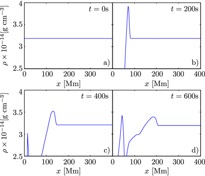
Figure 8: Density profiles at the chromospheric surface for different times showing the evolution of the Moreton wave. The magnetic field strength is $B_{0}=1$ G and the pressure pulse is $50$ times larger than the ambient pressure.

Thus, in order to analyze the chromospheric disturbance we evaluate the density profile considering an “adaptive” interface corona-chromosphere. This is, we adjust the measurement to the downward movement of the chromospheric surface. Also, instead of simply taking the density values considering a single layer of computational cells, just below the interface, we construct a profile using the average density over a vertical region below the chromospheric surface. As the H$\alpha$ core emission measure in the upper chromosphere is mainly sensitive to the density disturbance (Leenaarts et al., 2012), this method is better adjusted to the observations and allows a more precise comparison. In Figure 9a-d we show the density profiles for the same experiment as in Figure 8a-d, considering a chromospheric vertical region of $d=1$ Mm (measured downwards from the upper layer), for the average density calculation. Note, the qualitative agreement with the observational profiles consisting on a leading density enhancement (the Moreton wave) followed by an irregular trend (Balasubramaniam et al., 2010) (the “activated” region behind the front, corresponding to the vertical shock compression over the chromosphere, see also the H$\alpha$ line center in Figure 3 of White et al. (2014)). The differentiated two step behavior can be appreciated from the figure. The vertical line separates the static region from the other one where the Moreton traveling perturbation can be appreciated.

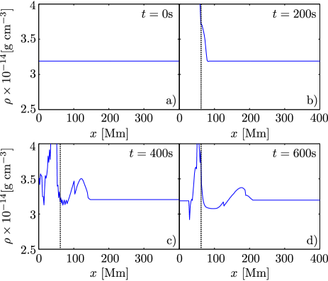
Figure 9: As Figure 8, considering an adaptive chromospheric surface and an average density for a vertical distance of $d=1$ Mm. The magnetic field strength is $B_{0}=1$ G and the pressure pulse is $50$ times larger than the ambient pressure.

The temporal piston

As noted before, the coronal shock speed is mainly determined by the magnetic field and almost independent of the pressure pulse intensity and the compression ratio (see Figure 7a-b). The speeds of the chromospheric perturbations will also be mostly determined by the magnetic field as they are supposed to be the consequence of the coronal shock sweeping over the chromospheric surface. However, a requirement for the perturbations to be observed is that the chromosphere is compressed beyond an instrumental threshold. Thus, it could happen that a very strong instantaneous pulse, not consistent with the plasma parameters, is required to produce a detectable perturbation. An alternative is to assume that the Moreton wave is triggered by a less intense pulse acting for a short time, i.e., a temporal piston.

As in Figure 7a-b, in Figure 10a-b we show the coronal mean compression ratio and the mean shock speed, now as a function of the pulse duration. Note from Figure 10b, that the mean shock speed is also approximately independent of the pulse duration, i.e., is fundamentally determined by the magnetic field value. The speed initial values of Figure 10b (at $t=0$ s) are the same as the ones of Figure 7b for an instantaneous pulse intensity of $1000$. Also, varying the duration of the pulse, from its instantaneous value to another of $50$ s duration the compression rate increases up to $\sim 100\%$.

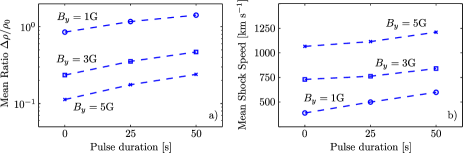
Figure 10: As Figure 7, coronal mean compression ratio a) and velocity b) for the shock wave considering different values of the magnetic field strength as a function of the pulse duration with $\Delta p/p=1000$.

The December 6, 2006 event

We now consider the Moreton wave event on December 6, 2006. The aim of this analysis is to reproduce the observational curve obtained in Francile et al. (2013) for the time-distance relation displayed in Figure 1. As seen previously, the main parameter required to determine the coronal shock speed is the magnetic field strength. To estimate this value we assume that the Moreton wave is due to a freely propagating coronal shock, which gradually decays to an ordinary fast-mode wave (Warmuth et al., 2001, 2004b). Considering the observational power law curve $D$ of the Moreton wave given by Figure 1, with the wave velocity corresponding to the later linear trend (at $t\geq$ 18:49 UT) we can calculate the required magnetic field strength of $B_{0}\approx 3.53$ G for a fast magnetosonic speed $v_{fm}\approx 720$ km s^-1. A distance of $35$ Mm -between the pressure pulse location and the chromospheric surface- is required to reproduce the phenomenological delay time between the flare ignition and the emergence of the chromospheric disturbance, i.e., $\sim 100$ s. We assumed a coronal temperature of $T=1.6$ MK and a coronal number density of $n=1.2\times 10^{8}$ cm^-3. The pressure pulse intensity is a crucial parameter in the simulation since it needs to be able to compensate the effect of the large magnetic field (associated with lower compression ratio values, see Figure 7a) and produce a sufficiently strong compression wave in the chromosphere to be detected by the HASTA telescope. The measurement of the detectable perturbation is performed by analyzing if the density perturbation over the interface corona-chromosphere is larger than the threshold value starting from the larger distances towards the smaller ones for each time. Considering these requirements we firstly used the maximum admisible temperature and density values to set the pressure inside the flaring region which corresponded to $\Delta p/p\approx 10000$, the larger values in Figure 7.

Figure 11 (blue circles) shows the obtained Moreton wave trajectory for $B_{0}=3.53$ G. The dashed line corresponds to the observational data reported in Francile et al. (2013) and the circles indicate the Moreton wavefront obtained in our simulation. We assume that radiative losses can be treated supposing that the upper chromospheric region is an optically thin media (see e.g., Gayley & Canfield (1991)). Thus, we considered that the emission measure is proportional to the square of the particle density. The data indicating a Moreton front are the perturbations beyond the threshold. They are obtained measuring the data from the larger to the smaller distances. The final detection of the Moreton perturbation occurs when the intensity has weakened below the threshold ($t\sim 450$ s). The circles corresponding to later times in Figure 11, ($\sim 420$ s $<t<\sim 500$ s) represent the stationary depression produced by the persistent vertical coronal compression (first step). These features were reported as persistent static brightenings and correspond to chromospheric H$\alpha$ features (Delannée et al., 2007; White et al., 2014). In Francile et al. (2013) we find that the Moreton wave is detected $130$ Mm away from the radiant point. Accordingly, in our simulations, this distance ($\sim 120$ Mm) corresponds to a peak of the perturbation. Considering the evolution at different times we obtain, as in White et al. (2014), that the chromospheric perturbation of December 2006, displays a characteristic down-up vertical velocity pattern that lags $\approx 50$ Mm behind the coronal signal and travels with almost the same speed and trajectory as the coronal one (see Figure 5). Large values of pressure pulses can be expected coming from super-Alfvénic reconnection outflows as mentioned by Mann & Warmuth (2011). However, less impulsive phenomenon could be accomplished providing the energy to generate almost the same chromospheric perturbation if a less impulsive event lasts a larger time. The red circles in Figure 11 correspond to the less intense temporal piston case that adjusts the observational curve: $\Delta p/p\approx 1000$, applied during $40$ s which could resemble the action of the expanding flanks of a CME (Temmer et al., 2009). This pulse duration corresponds to the minimum value that produces a compression ratio beyond the instrumental threshold.

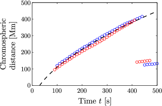
Figure 11: Comparison between the observational curve and the numerical simulation for $B_{0}=3.53$ G. The dashed line represents the 2D averaged chromospheric distance traveled by the Moreton wave registered on December 6, 2006 by Francile et al. (2013). The blue and red circles indicate the traveling wavefront obtained by the simulation applying an instantaneous pressure pulse of $\Delta p/p\approx 10000$ and a temporal pressure pulse of $\Delta p/p\approx 1000$, applied during $40$ s, respectively. A threshold of $8\%$ in the compression ratio of an optically thin media is considered.

Conclusions

Figure 11 shows that the kinematics of the Moreton event of December 6, 2006 can be reproduced assuming a blast-wave scenario, originated from a single source, that produces a coronal fast mode MHD shock that sweeps the chromosphere generating the Moreton perturbation. This source could be generated by a flare that ignites the blast-wave or by the expansion of CME flanks due to the flare ignition. We found that, using typical coronal and chromospheric parameters, a wave of large amplitude that propagates decelerating (starting with an initial $a_{0}\geq-30$ km s^-2) with a decreasing amplitude until it acquires a final fast magnetosonic free speed linear trend of $v_{fm}\approx 720$ km s^-1 is obtained. As in White et al. (2014) and in Francile et al. (2013) we found that the chromospheric perturbation displays a characteristic down-up vertical velocity pattern that lags behind the coronal signal and travels with the same speed and trajectory as the coronal one (see Figure 5). A uniform magnetic field value of $B_{0}\approx 3.53$ G and a distance of $35$ Mm, between the pressure pulse location and the corona-chromospheric interface, are required to reproduce the phenomenological delay time between the flare ignition and the emergence of the chromospheric disturbance. The first detection of the Moreton wavefront is $\approx 120$ Mm far from the radiant point which is consistent with the value obtained in Francile et al. (2013).

It has been argued that the flare explosion alone is not enough to give account of the Moreton event due to the discrepancy between the frequency of flare phenomenon and the relatively rare observations of coronal shocks. Thus, another mechanism would be necessary or a very special condition must be accomplished to give account of the shock formation that produces the large-scale Moreton event. If the modeling used here is an accurate one, our results show that, given typical coronal and chromospheric parameters, a set of limiting conditions are required to obtain both, a final linear trend associated with a fast magnetosonic speed and a strong pressure pulse able to generate a detectable compression ratio. The final fast magnetosonic free speed requires a definite magnetic field intensity (Figure 7b), but if the intensity of the magnetic field is large the compression ratio values are small and hinder the wave detection (Figure 7a). Accordingly, as seen in the Appendix, the flare expansion should be located at the periphery of the AR in order to avoid large magnetic field values (where $\beta\sim 1\times 10^{-4}$). Also, the fact that a very strong pressure pulse (limited by the admissible values of temperature and density) was required to obtain an emission enhancement of only $8$% for later times reinforces the argument.

Appendix A Importance of the $\beta$ parameter to ignite a coronal shock

Consider a steady shock plane-parallel to the magnetic field ($B_{0}$) and normal to the $x$-coordinate. Making use of the Rankine-Hugoniot conditions, the conservation laws for mass, momentum, energy and magnetic flux read (see for example Torrilhon (2003) and Draine (2011)):

$$\begin{array}[]{rcl}&\rho_{0}v_{0}=\rho_{1}v_{1},&\\ &v_{0}B_{0}=v_{1}B_{1},&\\ &\rho_{0}v_{0}^{2}+p_{0}+\frac{B_{0}^{2}}{8\pi}=\rho_{1}v_{1}^{2}+p_{1}+\frac{B_{1}^{2}}{8\pi},&\\ &v_{0}\left[\frac{1}{2}\rho_{0}v_{0}^{2}+\frac{\gamma}{\gamma-1}v_{0}p_{0}+v_{0}\frac{B_{0}^{2}}{8\pi}\right]=&\\ &=v_{1}\left[\frac{1}{2}\rho_{1}v_{1}^{2}+\frac{\gamma}{\gamma-1}v_{1}p_{1}+v_{1}\frac{B_{1}^{2}}{8\pi}\right]&\\ \end{array}$$ (5)

where the subscripts $0$ and $1$ denote preshock and postshock conditions, respectively, $v$ is the velocity in $x$-direction in a frame fixed to the shock front.

The non-trivial solution is one that produces different values on each side of the discontinuity. Considering the preshock plasma at rest, it results that $v_{0}=v_{s}$ in the moving frame, where $v_{s}$ is the shock speed. Defining the compression ratio $X=\rho_{1}/\rho_{0}$ (Draine, 2011):

$$\begin{array}[]{rcl}2(2-\gamma)X^{2}+\gamma\left[(\gamma-1)\beta M_{s}^{2}+2(1+\beta)\right]X-\\ \\ \gamma(\gamma+1)\beta M_{s}^{2}=0\end{array}$$ (6)

$M_{s}=v_{s}/c_{s}$ is the shock Mach number.

As the shock speed is equal or larger than the fast magnetosonic speed $v_{fm}=\left(v_{A}^{2}+c_{s}^{2}\right)^{1/2}$, a shock compression implies $v_{s}=\alpha v_{fm}$, where $\alpha\geq 1$, thus:

$$M_{s}^{2}=\alpha^{2}\frac{v_{A}^{2}+c_{s}^{2}}{c_{s}^{2}}=\alpha^{2}\left[\frac{2}{\gamma\beta}+1\right].$$ (7)

We can rewrite Eq. 6 in terms of the parameter $\beta$

$$\begin{array}[]{rcl}2(2-\gamma)X^{2}+\left[\alpha^{2}(\gamma-1)(2+\gamma\beta)+2(1+\beta)\right]X-\\ \\ \alpha^{2}(\gamma+1)(2+\gamma\beta)=0.\end{array}$$ (8)

Note that, in the case of interest ($1\leq\gamma\leq 2$), Eq. 8 has only one positive root which satisfies $X\geq 1$. The limit $X\rightarrow 1$, is obtained when $\beta\rightarrow 0$, independently of the values of $\gamma$ and $\alpha$. Thus, the flare-associated pressure pulse cannot ignite a shock wave in strong field regions where $\beta\rightarrow 0$. A detailed study on MHD shock wave formation can be found in Vršnak & Lulić (2000a) and Vršnak & Lulić (2000b).

References

- Aschwanden (2005) Aschwanden M. J., 2005, Physics of the Solar Corona. An Introduction with Problems and Solutions (2nd edition)
- Athay & Moreton (1961) Athay R. G., Moreton G. E., 1961, ApJ, 133, 935
- Aurass et al. (2002) Aurass H., Shibasaki K., Reiner M., Karlický M., 2002, ApJ, 567, 610
- Balasubramaniam et al. (2010) Balasubramaniam K. S., et al., 2010, ApJ, 723, 587
- Cécere et al. (2012) Cécere M., Schneiter M., Costa A., Elaskar S., Maglione S., 2012, ApJ, 759, 79
- Chen & Shibata (2000) Chen P. F., Shibata K., 2000, ApJ, 545, 524
- Chen et al. (2002) Chen P. F., Wu S. T., Shibata K., Fang C., 2002, ApJ, 572, L99
- Chen et al. (2005) Chen P. F., Ding M. D., Fang C., 2005, Space Sci. Rev., 121, 201
- Cliver et al. (1999) Cliver E. W., Webb D. F., Howard R. A., 1999, Sol. Phys., 187, 89
- Costa et al. (2009) Costa A., Elaskar S., Fernández C. A., Martínez G., 2009, MNRAS, 400, L85
- Delaboudinière et al. (1995) Delaboudinière J.-P., et al., 1995, Sol. Phys., 162, 291
- Delannée et al. (2007) Delannée C., Hochedez J.-F., Aulanier G., 2007, A&A, 465, 603
- Draine (2011) Draine B. T., 2011, Physics of the Interstellar and Intergalactic Medium
- Fernández et al. (2009) Fernández C. A., Costa A., Elaskar S., Schulz W., 2009, MNRAS, 400, 1821
- Francile et al. (2013) Francile C., Costa A., Luoni M. L., Elaskar S., 2013, A&A, 552, A3
- Fryxell et al. (2000) Fryxell B., et al., 2000, ApJS, 131, 273
- Gayley & Canfield (1991) Gayley K. G., Canfield R. C., 1991, ApJ, 380, 660
- Gilbert & Holzer (2004) Gilbert H. R., Holzer T. E., 2004, ApJ, 610, 572
- Gilbert et al. (2008) Gilbert H. R., Daou A. G., Young D., Tripathi D., Alexander D., 2008, ApJ, 685, 629
- Guo et al. (2013) Guo L.-J., Bhattacharjee A., Huang Y.-M., 2013, ApJ, 771, L14
- Handy et al. (1999) Handy B. N., et al., 1999, Sol. Phys., 187, 229
- Knock et al. (2001) Knock S. A., Cairns I. H., Robinson P. A., Kuncic Z., 2001, J. Geophys. Res., 106, 25041
- Lee et al. (2009) Lee D., Deane A. E., Federrath C., 2009, in Pogorelov N. V., Audit E., Colella P., Zank G. P., eds, Astronomical Society of the Pacific Conference Series Vol. 406, Numerical Modeling of Space Plasma Flows: ASTRONUM-2008. p. 243
- Leenaarts et al. (2007) Leenaarts J., Carlsson M., Hansteen V., Rutten R. J., 2007, A&A, 473, 625
- Leenaarts et al. (2012) Leenaarts J., Carlsson M., Rouppe van der Voort L., 2012, ApJ, 749, 136
- Magdalenić et al. (2012) Magdalenić J., Marqué C., Zhukov A. N., Vršnak B., Veronig A., 2012, ApJ, 746, 152
- Mann & Warmuth (2011) Mann G., Warmuth A., 2011, A&A, 528, A104
- Mei et al. (2012) Mei Z., Shen C., Wu N., Lin J., Murphy N. A., Roussev I. I., 2012, MNRAS, 425, 2824
- Moreton (1960) Moreton G. E., 1960, AJ, 65, 494
- Moreton & Ramsey (1960) Moreton G. E., Ramsey H. E., 1960, PASP, 72, 357
- Onofri et al. (2004) Onofri M., Primavera L., Malara F., Veltri P., 2004, Physics of Plasmas, 11, 4837
- Su et al. (2015) Su W., Cheng X., Ding M. D., Chen P. F., Sun J. Q., 2015, ApJ, 804, 88
- Temmer et al. (2009) Temmer M., Vršnak B., Žic T., Veronig A. M., 2009, ApJ, 702, 1343
- Thompson et al. (1998) Thompson B. J., Plunkett S. P., Gurman J. B., Newmark J. S., St. Cyr O. C., Michels D. J., 1998, Geophys. Res. Lett., 25, 2465
- Torrilhon (2003) Torrilhon M., 2003, Journal of Plasma Physics, 69, 253
- Uchida (1968) Uchida Y., 1968, Sol. Phys., 4, 30
- Uchida et al. (1973) Uchida Y., Altschuler M. D., Newkirk Jr. G., 1973, Sol. Phys., 28, 495
- Vršnak & Cliver (2008) Vršnak B., Cliver E. W., 2008, Sol. Phys., 253, 215
- Vršnak & Lulić (2000a) Vršnak B., Lulić S., 2000a, Sol. Phys., 196, 157
- Vršnak & Lulić (2000b) Vršnak B., Lulić S., 2000b, Sol. Phys., 196, 181
- Vršnak et al. (2002a) Vršnak B., Warmuth A., Brajša R., Hanslmeier A., 2002a, A&A, 394, 299
- Vršnak et al. (2002b) Vršnak B., Magdalenić J., Aurass H., Mann G., 2002b, A&A, 396, 673
- Warmuth et al. (2001) Warmuth A., Vršnak B., Aurass H., Hanslmeier A., 2001, ApJ, 560, L105
- Warmuth et al. (2004a) Warmuth A., Vršnak B., Magdalenić J., Hanslmeier A., Otruba W., 2004a, A&A, 418, 1101
- Warmuth et al. (2004b) Warmuth A., Vršnak B., Magdalenić J., Hanslmeier A., Otruba W., 2004b, A&A, 418, 1117
- Warmuth et al. (2005) Warmuth A., Mann G., Aurass H., 2005, ApJ, 626, L121
- White et al. (2014) White S., Balasubramaniam K., Cliver E., 2014, AFRL-RV-PS-TP-2014-0004. Air Force Research Laboratory, Preprint - Technical Paper, 22
- Wu et al. (2001) Wu S. T., Zheng H., Wang S., Thompson B. J., Plunkett S. P., Zhao X. P., Dryer M., 2001, J. Geophys. Res., 106, 25089
- Zhang et al. (2011) Zhang Y., Kitai R., Narukage N., Matsumoto T., Ueno S., Shibata K., Wang J., 2011, PASJ, 63, 685
- Zhukov (2011) Zhukov A. N., 2011, Journal of Atmospheric and Solar-Terrestrial Physics, 73, 1096
- Zhukov & Auchère (2004) Zhukov A. N., Auchère F., 2004, A&A, 427, 705