Imprint of a 2 Million year old source on the cosmic ray anisotropy

Abstract

We study numerically the anisotropy of the cosmic ray (CR) flux emitted by a single source calculating the trajectories of individual CRs. We show that the contribution of a single source to the observed anisotropy is determined solely by the fraction the source contributes to the total CR intensity, its age and its distance, and does not depend on the CR energy at late times. Therefore the observation of a constant dipole anisotropy indicates that a single source dominates the CR flux in the corresponding energy range. A natural explanation for the plateau between 2–20 TeV observed in the CR anisotropy is thus the presence of a single, nearby source. For the source age of 2 Myr, as suggested by the explanation of the antiproton and positron data from PAMELA and AMS-02 through a local source, we determine the source distance as $\sim 200$ pc. Combined with the contribution of the global CR sea calculated in the escape model, we can explain qualitatively the data for the dipole anisotropy. Our results suggest that the assumption of a smooth CR source distribution should be abandoned between $\simeq 200$ GeV and 1 PeV.

1. Introduction

The observed intensity of cosmic rays (CR) is characterised by a large degree of isotropy up to the highest energies. The measured dipole anisotropy $\delta$ increases up $E\sim 2$ TeV, forms an approximately energy independent plateau between $E\sim 2$–20 TeV, before the amplitude decreases again. Finally, at energies $E\raise 1.29167pt\hbox{$\;>$\kern-7.5pt\raise-4.73611pt\hbox{$\sim\;$}}100$ TeV, the anisotropy grows fast with energy. Such a behavior of the dipole anisotropy $\delta$ as function of energy seems at first sight difficult to reconcile with diffusive CR propagation: In this picture, the scattering of CRs on inhomogeneities of the Galactic magnetic field (GMF) converts their trajectories to a random walk, erasing thereby most directional information. Cosmic rays are most effectively scattered by those turbulent field modes whose wave-length equal their Larmor radii. Therefore the scattering rate is energy dependent and determined by the fluctuation spectrum of the turbulent GMF. As result, both the diffusion coefficient and the CR anisotropy are expected to increase with energy. This picture is supported e.g. by recent data from the AMS-02 experiment for the B/C ratio which are consistent with the simple power-law $D(E)\propto E^{0.31}$ up to the rigidity 1.8 TV.

In the diffusion approximation, Fick’s law is valid and the net CR current $\boldsymbol{j}(E)$ is determined by the gradient of the CR number density $n(E)={\rm d}N/({\rm d}E{\rm d}V)$ and the diffusion tensor $D_{ab}(E)$ as $j_{a}=-D_{ab}\nabla_{b}n$. The dipole vector $\boldsymbol{\delta}$ of the CR intensity $I=c/(4\pi)n$ follows then as

$$\delta_{a}=\frac{3}{c}\frac{j_{a}}{n}=-\frac{3D_{ab}}{c}\frac{\nabla_{b}n}{n}\,.$$ (1)

Within this approximation, the diffusion tensor $D_{ab}$ is an external input. The traditional approach to determine $D_{ab}$ as a function of the assumed magnetic field uses kinetic theory, see e.g. Berezinskii et al. (1990). Such an analytical approach allows one to connect both $D_{ab}$ and $\delta_{a}$ to the spectrum of magnetic field fluctuations, involves however the use of approximations.

An alternative method uses the trajectories of individual CRs calculated numerically solving the Lorentz equation in turbulent and regular magnetic fields. This approach is numerically expensive and has been restricted mainly to the calculation of the diffusion tensor $D_{ab}$ (Giacalone & Jokipii, 1999; Casse et al., 2002; Giacinti et al., 2012a). Since the anisotropy in the astrophysically interesting cases is small, its calculation requires a much larger number of CR trajectories. Therefore the determination of the CR anisotropy expected from a smooth source distribution has not been feasible using this method directly. Instead, the approximation proposed by Karakula et al. (1972) has been widely used in the high-energy range, $E\raise 1.29167pt\hbox{$\;>$\kern-7.5pt\raise-4.73611pt\hbox{$\sim\;$}}10^{18}$ eV. In this letter, we concentrate on the case of a single source and show that the calculation of the anisotropy from first principles is possible for an interesting range of parameters.

The propagation of CRs can be divided into three different regimes: The free streaming, the anisotropic and the quasi-Gaussian diffusion of CRs. In the first regime, the change of the particle momentum is small. The intermediate regime of anisotropic diffusion was explored first by Giacinti et al. (2012a, 2013); a study of the anisotropy in this regime will be presented elsewhere. Here, we concentrate on the case of quasi-Gaussian diffusion and show that then the dipole anisotropy of a single source with age $T$ and distance $R$ is given by $\delta=3R/(2cT)$, independent of the regular and turbulent magnetic field. As an application of this result, we consider the observed CR dipole anisotropy. We propose as explanation for the plateau in the observed anisotropy between 2–20 TeV that a single nearby source dominates the CR flux in this energy range. At lower energies, the anisotropy decreases because the fraction of CRs contributed by the single source goes down. We show that the anisotropy data between 200 GeV and 4 PeV can be naturally explained by a local CR source with the age of 2 Myr and distance $\sim 200$ pc, consistent with the characteristics of the single source determined in Kachelrieß et al. (2015) for an explanation of the antiproton and positron data from PAMELA and AMS-02.

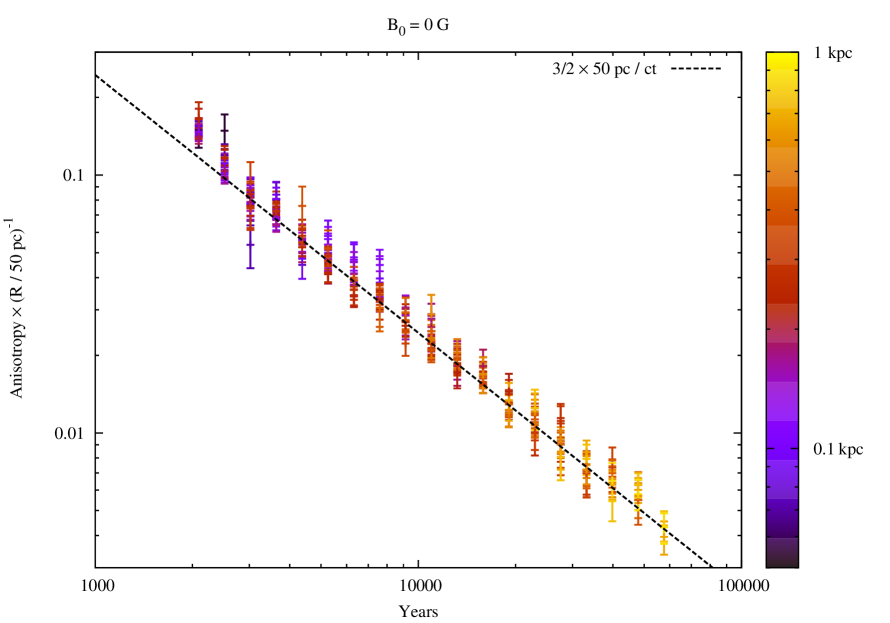
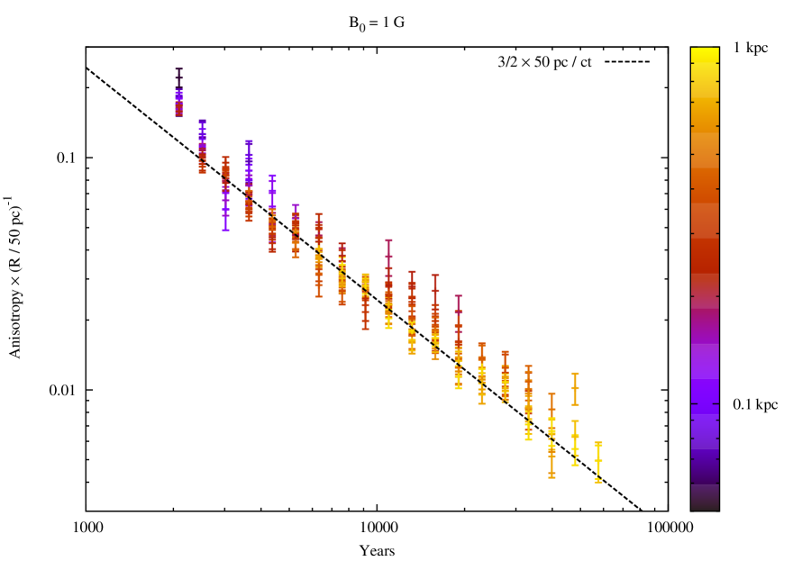
Figure 1.— The rescaled flux anisotropy $A$ of single sources at various distances as function of time. The distance is indicated by the color code in kpc. Left panel: turbulent magnetic field $B_{\rm rms}=0.3\,\mu$G; right panel: $B_{0}=1\,\mu$G and $B_{\rm rms}=0.3\,\mu$G.

2. Anisotropy in the quasi-Gaussian regime

We avoid the limitations of the diffusion approximation by calculating the trajectories of individual CRs in a given regular and turbulent magnetic field using the numerical code described by Giacinti et al. (2011, 2012b). We use as spectrum $\mathcal{P}(\boldsymbol{k})$ of the magnetic field fluctuations isotropic Kolmogorov turbulence, $\mathcal{P}(k)\propto k^{-\alpha}$ with $\alpha=5/3$ and set the maximum length $l_{\rm max}$ equal to 25 pc. For the numerical calculations, we use nested grids. This allows us to choose an effective $l^{\prime}_{\min}$ sufficiently small compared to the Larmor radius considered.

We model the CR source as an instantaneous injection of CRs at a single point. Since we are interested in the generic behavior of CR diffusion on relatively small length scales, we use not a concrete GMF model but approximate its regular component by a uniform field. We measure the momentum distribution $f(\boldsymbol{p})$ of CRs crossing a set of spheres with radii between 1 pc and 1 kpc centered on the CR source. We verify that in the quasi-Gaussian regime the distribution is compatible with a dipole, and compute the anisotropy $A$ of the flux of CRs crossing each sphere. The statistical error of the anisotropy estimate is a factor $1/A^{2}$ larger than the error of the corresponding flux estimate. Thus even for relatively large flux anisotropies, $A\simeq 0.01$, the number of trajectories and hence the CPU time required is increased by a factor $10^{4}$. The average total computing time used for a single run was about 10 CPU years. To further reduce the statistical uncertainty, we have averaged the anisotropy over regions selected according to the symmetry of the regular magnetic field $B_{0}$: spherical symmetry for $B_{0}=0$ and axial symmetry for $B_{0}={\rm const}$.

In the left panel of Fig. 1, we show the flux anisotropy $A$ of single sources at various distances as function of time for a purely turbulent magnetic field with strength $B_{\rm rms}=0.3\,\mu$G. We choose the times and length scales sufficiently large such that the CR propagation proceeds in the quasi-Gaussian regime, $t\gg 2D/c^{2}$ and $l\gg l_{\rm coh}$. For a purely turbulent field, CRs should perform a random walk. Thus their density is Gaussian, and as a result, Eq. (1) simplifies (Shen & Mao, 1971) to

$$A=\frac{R}{cT}\simeq 3.3\times 10^{-4}\left(\frac{R}{200\,{\rm pc}}\right)\left(\frac{T}{2\,{\rm Myr}}\right)^{-1}\,.$$ (2)

The flux anisotropy $A$ shown in Fig. 1 for sources at varying distances is rescaled to the value of the nearest source at 50 pc assuming the validity of Eq. (2). Within the numerical precision of our results, the obtained values for $A$ follow nicely the analytical result.

Next we add a regular field to the turbulent field. In this case, CRs diffuse faster parallel than perpendicular to the regular field lines and one may wonder, if the simple formula (2) for the dipole anisotropy still holds. Restricting ourselves again to the case $t\gg 2D/c^{2}$ and $l\gg l_{\rm coh}$, we confirm numerically that CR propagate also with a non-zero regular field in the quasi-Gaussian regime. Now the widths $4D_{i}t$ of the three-dimensional Gaussian describing the CR density $n(E,\boldsymbol{x})$ are given by the corresponding components of the diffusion tensor. Consequently, we expect that the regular field leads to strong deviations from a radially symmetric number density of CRs but does not influence the anisotropy. In the right panel of Fig. 1, we show our results for the flux anisotropy $A$ in the presence of both a turbulent and regular field, choosing as an example the field-strengths $B_{0}=1\,\mu$G and $B_{\rm rms}=0.3\,\mu$G. Comparing the results in the left (without) and the right (with regular field) panel, it is clear that the regular field has no impact on the anisotropy.

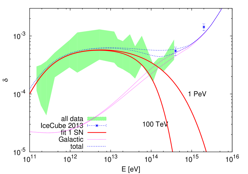
Figure 2.— Lower and upper limit (green band) on the dipole anisotropy and data from IceCube (blue errorbars) compared to the contribution from the local source (red, for two values of $E_{\max}$) and from the average CR sea (magenta) as function of energy.

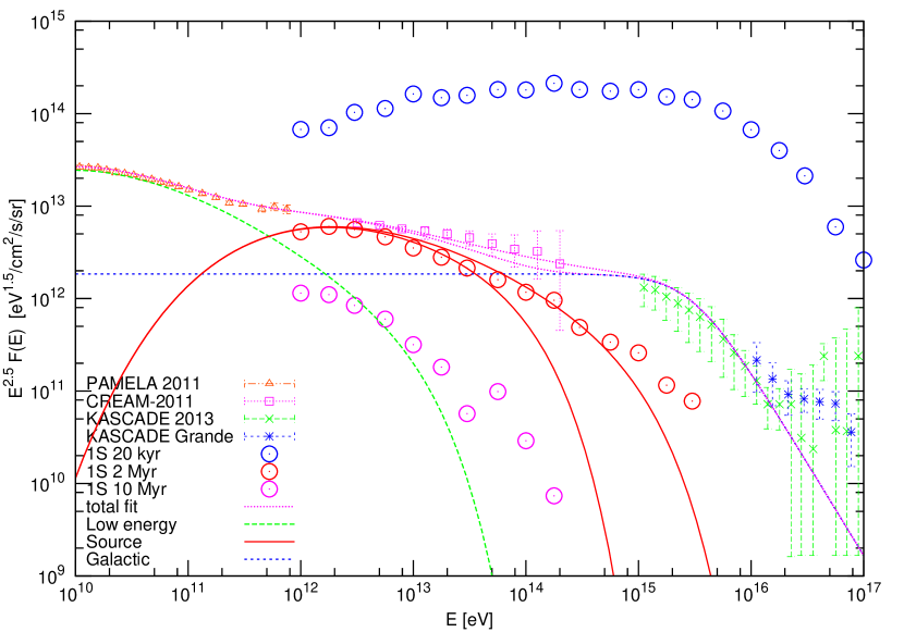
Figure 3.— Contribution from average Galactic (blue line), from the local source (red lines, for cutoff $E_{\max}=10^{14}$ and $10^{15}$ eV), and old local sources (green line) to the CR proton intensity together with experimental data (errorbars). Additionally, the flux from the local source is shown by dots for three source ages.

3. Interpretation of the observed CR anisotropy

In Fig. 2, we show as band the range of experimental data collected by Di Sciascio & Iuppa (2014) on the magnitude of the CR dipole anisotropy$\delta$ together with data from IceCube (blue errorbars) (Abbasi et al., 2012). The anisotropy grows as function of energy until $E\sim 2$ TeV, remains approximately constant in the range 2–20 TeV, before it decreases again. Starting from 100 TeV the anisotropy increases, with a rate which is consistent with one determined in the escape model of Giacinti et al. (2014, 2015).

In the standard diffusion picture, the anisotropy is connected to the gradient of the global CR sea density and the diffusion coefficient. Both quantities increase with energy and, consequently, the energy dependence shown in Fig. 2 is difficult to explain. Our results from the previous section suggest to connect the plateau in the dipole anisotropy between 2–20 TeV to the presence of a single nearby source. We determine the relative contribution to the total CR intensity from the nearby source, $f_{s}=I_{s}(E)/I_{\rm tot}$, and from the global CR sea using the fluxes from Kachelrieß et al. (2015). The contribution of the local source to the dipole anisotropy follows then as $\delta_{s}=3f_{i}R/(2cT)$. This anisotropy is shown with red lines in Fig. 2. Combined with $T\simeq 2$ Myr as age of the source, we can determine its distance as $R\simeq 200\,{\rm pc}\times\delta_{s}/(5\times 10^{-4})$.

Since the spread of the experimental data on the dipole is considerable, let us consider for illustration the following two extreme situations: First, the true dipole may be close to the lower limit of the measured range, $\delta\sim 3\times 10^{-4}$. In this case, the plateau extends up to $\simeq 10^{14}$ eV, the maximal energy of CRs accelerated in the local source is unrestricted and the source distance could be as low as 100 pc. The following rise of the dipole is then explained by the contribution of the global CR sea which we calculate in the escape model of Giacinti et al. (2014, 2015). In the other extreme, the true dipole may be close to the upper limit of the measurements, $\delta\sim 10^{-3}$. In this case, we have to introduce a cutoff $\exp(-E/E_{\max})$ in the energy of CRs accelerated in the local source such that their contribution to the total CR intensity and thus to the observed dipole decreases towards the EAS-Top value.

We can constrain these extreme choices considering also the total CR proton flux. In Fig. 3, we compare experimental results for the proton flux from CREAM (Yoon et al., 2011), PAMELA (Adriani et al., 2011), KASCADE and KASCADE-Grande (Apel et al., 2011), to the proton flux from the local source shown by dots and the average global CR sea at low energies (green line). Larger maximal values of $\delta$ require a lower value of $E_{\max}$, making the source spectrum more “bumpy”. Such a spectral distortion in the total proton flux is avoided for values of $E_{\max}\raise 1.29167pt\hbox{$\;>$\kern-7.5pt\raise-4.73611pt\hbox{$\sim\;$}}10^{14}$ eV, what also ensures that the antiproton data from AMS-02 can be explained.

Let us now comment on the decrease of the measured dipole anisotropy at low-energies, $\raise 1.29167pt\hbox{$\;<$\kern-7.5pt\raise-4.73611pt\hbox{$\sim\;$}}2$ TeV. A natural explanation for this decrease is a small off-set of the Earth with respect to magnetic field line going through the source. The perpendicular extension of the elongated volume filled with CRs by the source decreases with energy. Thus the lower end of the plateau is determined by the perpendicular distance of the Earth to the magnetic field line going through the source and is therefore a free parameter. In Fig. 3, we show the proton flux from the local source as a red line using $E_{\min}=10^{12}$ eV and $E_{\max}=10^{14}$ eV and $10^{15}$ eV as low- and high-energy cutoffs, respectively.

The difference at low energies between the observed CR flux and the one from the local source should be contributed by old, local sources. This contribution is shown for illustration in Fig. 3 as a green line, obtained by subtracting the two fluxes. Fry et al. (2015) showed that their age should be $T>14$ Myr. Therefore the high-energy CRs emitted by these sources escaped already, what might explain the suppression of their combined CR fluxes above $10^{11}$ eV. Their individual dipoles $\delta_{i}\propto f_{i}/T$ are smaller, should partially cancel in their sum, and we therefore neglect their contribution to the total dipole amplitude in Fig. 2. Since the number $N$ of sources contributing is large, the approximation of a smooth source distribution and thus also the standard approach used e.g. by Strong et al. (2007); Evoli et al. (2008); Putze et al. (2011) may be justified in this energy range. The transition between the single and many source regimes around $E\sim 2\times 10^{11}$ eV may be connected to the spectral breaks observed by PAMELA.

The phase of the first harmonics is almost constant up to 100 TeV energy (Di Sciascio & Iuppa, 2014), and changes thereafter fast. Such a behavior is natural in our model: At all energies $E\raise 1.29167pt\hbox{$\;<$\kern-7.5pt\raise-4.73611pt\hbox{$\sim\;$}}100$ TeV, the anisotropy is dominated by local source(s) which are located preferentially along the local magnetic field lines. As result, the dipole phase expected does not change its value up to 100 TeV, where the Galactic sea of CRs starts to dominate and thus the dipole direction is given by Eq. (1).

The presence of a nearby source dominating the CR flux and dipole in the TeV range is natural to expect (Kachelrieß et al., 2015): The average rate of SN explosions in the Milky Way is one SN per (0.3–3)$\times 10^{4}$ yr per kpc³. Cosmic rays in the TeV energy range fill a 100 pc wide, kpc long volume directed along the regular GMF lines for a time of a Myr. It is thus likely that one SN has exploded during the last Myr within this volume.

Such a source is consistent with the explanation for the deposition of ⁶⁰Fe isotopes in the deep ocean crust by the passage of an expanding shell of a 2 Myr old supernova remnant through the Solar System (Knie et al., 1999; Benitez et al., 2002; Fry et al., 2015). The distance determined by  Fry et al. (2015) e.g. for the case of a $25M_{\odot}$ core-collapse supernova is $\simeq 130$ pc. Relaxing some of the assumptions like an isotropic emission, this estimate may be compatible with our value $R\sim 200$ pc in case of a low dipole amplitude. Moreover, a single local source dominating the local CR proton spectrum explains the known differences in the slopes between CR protons and nuclei and the anomalous energy dependence of the spectra of positrons and antiprotons (Kachelrieß et al., 2015).

4. Discussion and Conclusions

The standard approach to CR propagation using either analytical (Berezinskii et al., 1990) or numerical methods (Strong & Moskalenko, 1998; Strong et al., 2007; Evoli et al., 2008) assumes a CR source distribution that is smooth in time and space. Blasi & Amato (2012a, b) based on earlier work by Lee (1979) studied the fluctuations in the CR density and the dipole induced by the stochastic nature of CR sources. Their results for the fluctuations diverge in the limit of small source distances and ages, $R_{\min},T_{\min}\to 0$. These divergences indicate that a statistical description of quantities like the CR dipole anisotropy in terms of its ensemble average and variance is not adequate, since the results depend strongly on the actual properties of the nearest source(s) in a given realization.

The strongly anisotropic diffusion of CRs that is typical for the GMF parameters favored by the escape model enhances these fluctuations: The majority of recent nearby sources is not connected to us by the regular field, and their contribution to the local CR intensity is therefore suppressed. In contrast, the flux of the single (or the few) sources active in the last few million years that are located in the volume aligned with the GMF lines passing near the Solar system is strongly enhanced. These effects prevent the mixing of CRs with energies 1-100 TeV of various sources into a “global, average CR sea,” and undermine thereby the basic assumption of a smooth, global CR distribution inherent in most approaches to Galactic CR physics.

We have shown that the dipole anisotropy in the CR flux emitted by a single source is independent of the turbulent and regular magnetic field and of the CR energy in the quasi-Gaussian regime. In particular, we have shown that the simple formula $A=R/(cT)$ for the dipole anisotropy holds also including a regular field. As an application we have considered the experimental data on the dipole anisotropy. We have argued that the approximately energy-independent plateau in the anisotropy around 2-20 TeV can be explained by the presence of a nearby CR source. The age and the distance of this source are compatible with the one required to explain the “anomalies” in the CR intensities of protons, antiprotons and positrons. If the source is also responsible for the observed ⁶⁰Fe overabundance in the million year old ocean crust, its distance should 100–200 pc, favoring thus values of the dipole anisotropy close to the lower end of the measured values.

Finally we note that our results can be used also to study the dipole anisotropy of the electron flux, constraining e.g. the contribution from recent pulsars, if energy losses are taken into account.

References

- Abbasi et al. (2012) Abbasi, R., et al. 2012, Astrophys.J., 746, 33, 1109.1017
- Adriani et al. (2011) Adriani, O., et al. 2011, Science, 332, 69, 1103.4055
- Apel et al. (2011) Apel, W., et al. 2011, Phys.Rev.Lett., 107, 171104, 1107.5885
- Benitez et al. (2002) Benitez, N., Maiz-Apellaniz, J., & Canelles, M. 2002, Phys.Rev.Lett., 88, 081101, astro-ph/0201018
- Berezinskii et al. (1990) Berezinskii, V., Bulanov, S., Dogiel, V., Ginzburg, V., & Ptuskin, V. 1990, Astrophysics of Cosmic Rays (North Holland)
- Blasi & Amato (2012a) Blasi, P., & Amato, E. 2012a, JCAP, 1201, 010, 1105.4521
- Blasi & Amato (2012b) ——. 2012b, JCAP, 1201, 011, 1105.4529
- Casse et al. (2002) Casse, F., Lemoine, M., & Pelletier, G. 2002, Phys.Rev., D65, 023002, astro-ph/0109223
- Di Sciascio & Iuppa (2014) Di Sciascio, G., & Iuppa, R. 2014, 1407.2144
- Evoli et al. (2008) Evoli, C., Gaggero, D., Grasso, D., & Maccione, L. 2008, JCAP, 0810, 018, 0807.4730
- Fry et al. (2015) Fry, B. J., Fields, B. D., & Ellis, J. R. 2015, Astrophys.J., 800, 71, 1405.4310
- Giacalone & Jokipii (1999) Giacalone, J., & Jokipii, J. R. 1999, ApJ, 520, 204
- Giacinti et al. (2012a) Giacinti, G., Kachelrieß, M., & Semikoz, D. 2012a, Phys.Rev.Lett., 108, 261101, 1204.1271
- Giacinti et al. (2013) ——. 2013, Phys.Rev., D88, 023010, 1306.3209
- Giacinti et al. (2014) ——. 2014, Phys.Rev., D90, 041302, 1403.3380
- Giacinti et al. (2015) ——. 2015, Phys.Rev., D91, 083009, 1502.01608
- Giacinti et al. (2011) Giacinti, G., Kachelrieß, M., Semikoz, D., & Sigl, G. 2011, Astropart.Phys., 35, 192, 1104.1141
- Giacinti et al. (2012b) ——. 2012b, JCAP, 1207, 031, 1112.5599
- Kachelrieß et al. (2015) Kachelrieß, M., Neronov, A., & Semikoz, D. 2015, 1504.06472
- Karakula et al. (1972) Karakula, S., Osborne, J., Roberts, E., & Tkaczyk, W. 1972, J.Phys., A5, 904
- Knie et al. (1999) Knie, K., Korschinek, G., Faestermann, T., Wallner, C., Scholten, J., et al. 1999, Phys.Rev.Lett., 83, 18
- Lee (1979) Lee, M. A. 1979, ApJ, 229, 424
- Putze et al. (2011) Putze, A., Maurin, D., & Donato, F. 2011, A&A, 526, A101, 1011.0989
- Shen & Mao (1971) Shen, C. S., & Mao, C. Y. 1971, Astrophys. Lett., 9, 169
- Strong & Moskalenko (1998) Strong, A., & Moskalenko, I. 1998, Astrophys.J., 509, 212, astro-ph/9807150
- Strong et al. (2007) Strong, A. W., Moskalenko, I. V., & Ptuskin, V. S. 2007, Ann.Rev.Nucl.Part.Sci., 57, 285, astro-ph/0701517
- Yoon et al. (2011) Yoon, Y., Ahn, H., Allison, P., Bagliesi, M., Beatty, J., et al. 2011, Astrophys.J., 728, 122, 1102.2575