Approximating the Ising model on fractal lattices
of dimension below two

Abstract

We construct periodic approximations to the free energies of Ising models on fractal lattices of dimension smaller than two, in the case of zero external magnetic field, using a generalization of the combinatorial method of Feynman and Vodvickenko. Our procedure is applicable to any fractal obtained by the removal of sites of a periodic two dimensional lattice. As a first application, we compute estimates for the critical temperatures of many different Sierpinski carpets and we compare them to known Monte Carlo estimates. The results show that our method is capable of determining the critical temperature with, possibly, arbitrary accuracy and paves the way to determine $T_{c}$ for any fractal of dimension below two. Critical exponents are more difficult to determine since the free energy of any periodic approximation still has a logarithmic singularity at the critical point implying $\alpha=0$. We also compute the correlation length as a function of the temperature and extract the relative critical exponent. We find $\nu=1$ for all periodic approximation, as expected from universality.

Preprint : CP3-Origins-2015-014 DNRF90 & DIAS-2015-14

I Introduction

Ising on fractals.

The well known exact solutions of the Ising model in one and two dimensions are the only exact solutions we have to date Ising:1925em ; Onsager_1944 . Ising models on fractals of dimension between one and two are natural possible candidates to enter this restricted group of solvable models. Actually, we already have solutions on some fractals, those with finite ramification number like the Sierpinski gasket, but these are of limited interest since they resemble the one dimensional case as they do not possess any phase transition at finite temperature gefen_1984 . Instead, a fractal with infinite ramification number as the Sierpinski carpet, which we know has a non-zero critical temperature Shinoda_2002 ; vezzani:2003aa , has to date been studied mostly numerically, and few analytical studies are available. In this paper we try to fill this gap presenting an analytical study of the Ising model on fractals of dimension below two, which include both the gasket and the carpet. We present a method in principle able to determine the critical temperatures exactly for all these fractals. Our approach is based on approximating the Ising model on non-periodic fractal lattices with a sequence of Ising models on periodic lattices. We do this by exploiting our ability to readily solve the two dimensional Ising model on an arbitrary periodic lattice using an extension of the combinatorial method of Feynman–Vodvickenko Vodvicenko_1965 ; Feynman_1972 ; Codello2010 .

Universality.

The understanding of universality classes in dimension equal or above two is now quite robust, in particular for system with $\mathbb{Z}_{2}$ symmetry Codello:2012sc ; El-Showk:2013nia . Less clear is the situation in dimension below two and greater than one. Continuous methods Guida:1998bx ; Ballhausen:2003gx give a fairly good description, and in some dimensions real space renormalization group studies are available Bonnier_1988 ; Monceau_2003 , but an explicit solution of the Ising model in some fractal case will provide strong indication regarding the reliability or not of continuous methods in dimension below two. In fact it is not completely clear if there is a difference between the values of critical exponents one can obtain with continuous methods, which usually make a continuation of the integer number of dimensions to fractional values, and the actual values obtained studying the analogous systems defined directly on lattices of non-integer fractal dimension. Another open question is if there is a lower critical dimension for the $\mathbb{Z}_{2}$ universality class, or even if this concept is well defined since it might be that universality depends on the fine details of the fractal gefen:1980aa . To clarify all these question, a better understanding of the Ising model in fractal dimension, which is a representative of the $\mathbb{Z}_{2}$ universality class, will be of the utmost significance. A further reason why the Ising model universality class is interesting in dimension below two is because it is the only non-trivial one in the family of the $O(N)$ models due to the generalised Mermin-Wagner theorem Cassi_1992 .

Summary of the paper.

In Section II we explain how to generalize the combinatorial method of Feynman and Vodvickenko to arbitrary periodic lattices. Then, in Section III, we explain how to apply it to approximate fractals. After some analytical results, we turn to numerical methods to extract the approximate critical temperatures and correlation lengths for many different fractals. We finally compare our results with the numerous existing Monte Carlo estimates available in the literature and we briefly discuss possible future applications of our method.

II Solution on arbitrary periodic lattices

II.1 The model

Definitions.

We briefly review the definitions that specify the model. We consider an arbitrary periodic lattice $\Lambda$ where at every lattice site $i$ there is a spin variable $\sigma_{i}\in\{-1,1\}$ and we define a microstate by a spin configuration $\{\sigma\}$. We assume nearest neighbour interactions so that the energy of a given spin configuration is given by

$$E\{\sigma\}=-J\sum_{\left\langle i,j\right\rangle}\sigma_{i}\sigma_{j}\,.$$ (1)

If $J>0$ the interaction is ferromagnetic, while it is antiferromagnetic if $J<0$. The partition function is the sum over all spin configurations weighted by the Boltzmann-Gibbs factor

$$Z_{\Lambda}=\sum_{\{\sigma\}}\exp\Big{\{}\beta\sum_{\left\langle i,j\right\rangle}\sigma_{i}\sigma_{j}\Big{\}}\,.$$ (2)

We define $\beta=1/k_{B}T$, where $k_{B}$ is the Boltzmann constant, and we set $J=1$ since we are going to consider only ferromagnetic interactions.

High temperature expansion.

Using the high temperature expansion, the partition function (2) can be rewritten as

$$Z_{\Lambda}=2^{N}\left(\cosh\beta\right)^{N_{l}}\Phi_{\Lambda}(v)\,,$$ (3)

where $v=\tanh\beta$ and $N\equiv N_{s}$ is the total number of lattice sites while $N_{l}$ is the total number of links. The function $\Phi_{\Lambda}(v)$ is the generating function of the numbers which count the graphs with even vertices of a given length that can be drawn on the lattice $\Lambda$. In this way, the problem of solving the Ising model on $\Lambda$ is reduced to the combinatorial problem of counting even closed graphs on $\Lambda$. In the thermodynamic limit it is the function $\Phi_{\Lambda}(v)$ which develops the non-analyticity that characterises the continuous phase transition. For this reason in the following we will focus on it and disregard the pre–factors appearing in (3).

For high temperature expansion studies of the Ising model on fractals, see Fabio_1994 . As explained in the next section, we instead resum the high temperature series by generalizing the approach of Feynman–Vodvickenko.

II.2 Feynman–Vodvickenko method

Exact solution on arbitrary periodic lattices.

Feynman Feynman_1972 and Vodvicenko Vodvicenko_1965 introduced a trick to reduce the problem of counting closed graphs to a random walk problem. More precisely, the generating function $\Phi_{\Lambda}(v)$ can be computed by counting closed weighted random walks paths on $\Lambda$, where the weights are complex amplitudes constructed so that the mapping from the high temperature expansion to the random walk problem works out correctly Kac_Ward_1952 ; Sherman_1960 ; Morita_1985 ; Codello2010 .

From the knowledge of the transition matrix $\mathbb{W}_{\Lambda}$ of the random walk problem, one can determine the explicit form of the generating function from the following relation Codello2010 :

$$\Phi_{\Lambda}(v)=\exp\left\{\frac{N}{2}\int\frac{d^{2}k}{(2\pi)^{2}}\log\,\textrm{det}\left[\mathbb{I}-v\,\mathbb{W}_{\Lambda}(\mathbf{k})\right]\right\}\,,$$ (4)

where the $\mathbf{k}=(k_{x},k_{y})$ integration is over the region $0\leq k_{x}\leq 2\pi$ and $0\leq k_{y}\leq 2\pi$. The singular non-trivial part of the free energy for spin $\beta f_{\Lambda}=-\frac{1}{N}\log\Phi_{\Lambda}$ for the lattice $\Lambda$, can finally be written as

$$\beta f_{\Lambda}(v)=-\frac{1}{2}\int\frac{d^{2}k}{(2\pi)^{2}}\,\textrm{log}\,P_{\Lambda}(v,\mathbf{k})\,,$$ (5)

where we have defined the determinant

$$P_{\Lambda}(v,\mathbf{k})=\textrm{det}\left[\mathbb{I}-v\,\mathbb{W}_{\Lambda}(\mathbf{k})\right]\,.$$ (6)

The matrices $\mathbb{W}_{\Lambda}(\mathbf{k})$ are $m\times m$ matrices with $m=s\times l$, where $s$ is the number of sites in the basic tile and $l$ is the total number of links in the basic tile.

Critical temperature.

If a phase transition takes place, the critical temperature can be determined as the real solution of

$$P_{\Lambda}(v,0)=0\,,$$ (7)

in the range $0<v<1$. Solutions of equation (7) for all Archimedean and Laves lattices have been studied in Codello2010 . Equivalently, we can determine the critical $v$ as the inverse of the largest positive real eigenvalue of $\mathbb{W}_{\Lambda}(0)$. This characterisation is very useful when the computation of the characteristic polynomial (7) becomes too demanding. Near the critical point, and in terms of the reduced temperature $t=T/T_{c}-1$, the critical exponent $\alpha$ is defined by the scaling $f_{\Lambda}(t)\sim t^{2-\alpha}$. In particular, a logarithmic singularity of the free energy, as the one present in (5), is encoded in $\alpha=0$.

Correlation length.

The correlation length can be computed from the knowledge of the lattice mass since $\xi_{\Lambda}=1/m_{\Lambda}$. This last is defined by the following small momenta expansion of the determinant,

$$P_{\Lambda}(v,\mathbf{k})=Z_{\Lambda}(v)\,\Big{[}m^{2}_{\Lambda}(v)+k^{2}+O(k^{4})\Big{]}\,,$$ (8)

where $Z_{\Lambda}(v)\equiv\left.\frac{\partial}{\partial k^{2}}P_{\Lambda}(v,\mathbf{k})\right|_{k=0}$ is the wave function renormalization. The lattice mass can then be written as $m^{2}_{\Lambda}(v)=P_{\Lambda}(v,0)/Z_{\Lambda}(v)$ and the correlation length takes the form

$$\xi_{\Lambda}(v)=\sqrt{\frac{\left.\frac{\partial}{\partial k^{2}}P_{\Lambda}(v,\mathbf{k})\right|_{k=0}}{P_{\Lambda}(v,0)}}\,.$$ (9)

The correlation length critical exponent is defined by the relation $\xi_{\Lambda}\sim|t|^{-\nu}$ valid in the scaling region near the phase transition.

III Fractals

Approximate solutions on fractals.

We now want to use our ability of solving the Ising model on an arbitrary periodic lattice to find approximations to the same problem but on fractal lattices of fractal dimension below two.

We will study Sierpinski carpets that are defined in an iterative way. Let us consider a two dimensional $L\times L$ tile, where some of the squares have been removed: we call this the generator of the fractal. It is also the first iteration, $k=1$, of the sequence that defines the fractal. Then, given the sequence at iteration $k$, the next iteration, $k+1$, can be constructed by replacing every existing square at the $k^{\rm{th}}$ iteration with the generator. In the limit $k\to\infty$ this defines a fractal.

In our approach, the lattice $\Lambda_{k}$ at iteration $k$ is defined as the infinite repetition of the tiling obtained at level $k$. We assume the Ising model on the limiting fractal $\Lambda_{\infty}=\lim_{k\to\infty}\Lambda_{k}$ exhibits the same behaviour as the Ising model defined on the fractal. In other words, we approximate the fractal’s determinant $P_{\Lambda_{\infty}}(v,\mathbf{k})$ using periodic approximations

$$P_{\Lambda_{\infty}}(v,\mathbf{k})=\lim_{k\to\infty}P_{\Lambda_{k}}(v,\mathbf{k})\,.$$ (10)

Furthermore we define ${\rm sc}(L,b)_{1}$ to be the generator where from $L\times L$ tile a $b\times b$ square is removed from the center. Then ${\rm sc}(L,b)_{k}$ denotes the tiling at iteration $k$. For illustration see Figure 1. We will denote with ${\rm SC}(L,b)_{k}$ the lattice obtained by tessellation of the plane with tile ${\rm sc}(L,b)_{k}$. We will also study Sierpinski gaskets. Theirs generators are a $L\times L$ tile where a single $(L-1)\times(L-1)$ block has been removed. Sierpinski gaskets have a finite ramification number, i.e. one can remove arbitrarily large pieces by cutting a finite number of links.

We denote with $T_{k}$ the critical temperature of the lattice $\Lambda_{k}$ where $\Lambda$ is understood from the context and similarly for the correlation length $\xi_{k}$.

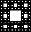
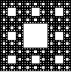
Figure 1: Illustration of ${\rm sc}(3,1)_{k}$ for $k=1,2,3,4$.

III.1 Sierpinski carpets

Explicit form of $\mathbb{W}$.

We can construct the transition matrix $\mathbb{W}_{\Lambda_{k}}(k_{x},k_{y})$ for any finite iteration Sierpinski carpet $\Lambda_{k}$ exactly. Explicitly, this can be constructed as the adjacency matrix of a weighted directed graph, in which each node of the graph represents one of the four directions $U,L,D,R$ associated to each site of the generator of $\Lambda_{k}$. In particular, when $k_{x}=k_{y}=0$ we can represent $\mathbb{W}_{\Lambda_{k}}(0,0)$ as the graph

$$U_{i,j} \overset{w_{i,j}}{\longrightarrow}U_{i-1,j} U_{i,j} \overset{w_{i,j}/\alpha}{\longrightarrow}L_{i-1,j} U_{i,j} \overset{\alpha w_{i,j}}{\longrightarrow}R_{i-1,j}$$

$$L_{i,j} \overset{\alpha w_{i,j}}{\longrightarrow}U_{i,j-1} L_{i,j} \overset{w_{i,j}}{\longrightarrow}L_{i,j-1} L_{i,j} \overset{w_{i,j}/\alpha}{\longrightarrow}D_{i,j-1}$$

$$D_{i,j} \overset{\alpha w_{i,j}}{\longrightarrow}L_{i+1,j} D_{i,j} \overset{w_{i,j}}{\longrightarrow}D_{i+1,j} D_{i,j} \overset{w_{i,j}/\alpha}{\longrightarrow}R_{i+1,j}$$

$$R_{i,j} \overset{w_{i,j}/\alpha}{\longrightarrow}U_{i,j+1} R_{i,j} \overset{\alpha w_{i,j}}{\longrightarrow}D_{i,j+1} R_{i,j} \overset{w_{i,j}}{\longrightarrow}R_{i,j+1}$$

where the indices are modulo $L$ and $\alpha=e^{i\frac{\pi}{4}}$ is the complex amplitude required by the Feynman-Vodvicenko method. Basically, in terms of directions, clockwise arrows have amplitude $\alpha$, counter clockwise arrows have amplitude $\alpha^{-1}$, while self connections have amplitude one. The weights $w_{i,j}$ are chosen equal to the matrix representation of the generator of the lattice $\Lambda_{k}$, setting $w_{i,j}=1$ if the site $(i,j)$ of the generator exists and $w_{i,j}=0$ if it is depleted. The case of the standard Ising model on square lattice can be represented as in Figure 2. The momentum dependence of $\mathbb{W}_{\Lambda_{k}}(k_{x},k_{y})$ is obtained by multiplying the links outgoing from $U$ with $e^{ik_{y}}$, from $L$ with $e^{ik_{x}}$, from $D$ with $e^{-ik_{y}}$, and from $R$ with $e^{-ik_{x}}$.

Although we are here interested in approximating fractals, by properly choosing $w_{i,j}$ this construction gives the transition matrix for any lattice with rectangular tile. For example, our construction encompasses the exact solution of the Ising model on all possible two dimensional depleted lattices, including the case of a random basic tile.

Standard Ising model.

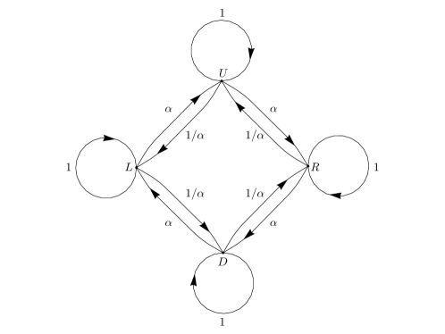
Figure 2: Graph representing the transition matrix $\mathbb{W}_{Ising}(0,0)$ for the standard Ising model on a square lattice.

We shortly review the solution of the standard two dimensional Ising model to exemplify the method. From Figure 2 we immediately reconstruct the transition matrix

$$\mathbb{W}_{Ising}(k_{x},k_{y})=\left(\begin{array}[]{cccc}e^{ik_{y}}&\frac{1}{\alpha}e^{ik_{y}}&0&\alpha e^{ik_{y}}\\ \alpha e^{ik_{x}}&e^{ik_{x}}&\frac{1}{\alpha}e^{ik_{x}}&0\\ 0&\alpha e^{-ik_{y}}&e^{-ik_{y}}&\frac{1}{\alpha}e^{-ik_{y}}\\ \frac{1}{\alpha}e^{-ik_{x}}&0&\alpha e^{-ik_{x}}&e^{-ik_{x}}\\ \end{array}\right)\,,$$ (15)

with $\alpha=e^{i\frac{\pi}{4}}$. The determinant is readily computed and gives the well known Onsager’s solution Onsager_1944 :

$$P_{Ising}(v,\mathbf{k})=\left(1+v^{2}\right)^{2}-2\,v\left(1-v^{2}\right)\Big{(}\!\cos k_{x}+\cos k_{y}\Big{)}\,.$$ (16)

Setting $P_{Ising}(v,0)=(1-2v-v^{2})^{2}=0$ gives $v_{c}=0.414214...$ as the only solution in the range $0<v<1$; this correspond to the critical temperature $T_{c}=2.26919...$ first computed by Kramer and Wannier using duality arguments Kramers_Wannier_1941 . Finally, using (9) we find the exact form for the correlation length

$$\xi_{Ising}(v)=2\sqrt{\frac{v-v^{3}}{\Big{(}1-2v-v^{2}\Big{)}^{2}}}\,,$$ (17)

which clearly diverges for $T\sim T_{c}$ since the denominator vanishes.

To check our formalism we can try to solve a redundant version of the two dimensional Ising model, defined on a tile of size $L>1$. With our previously defined notations, they are equivalent to ${\rm SC}(L,0)_{1}$. For example in the cases $L=2,3$ we find to following characteristic polynomials,

$$P_{\rm{SC}(2,0)_{1}}(v,0) = (1+v^{2})^{4}(1+2v-v^{2})^{2}(1-2v-v^{2})^{2}$$

$$P_{\rm{SC}(3,0)_{1}}(v,0) = (1-2v-v^{2})^{2}(1+2v+2v^{2}-2v^{3}+v^{4})^{4}(1-v+2v^{2}+v^{3}+v^{4})^{4}\,,$$ (18)

which indeed have only the $v_{c}=0.414214...$ solution in the range $0<v<1$. This represents a non-trivial check of our ability to construct the transition matrices for an arbitrary lattice. The momentum dependence becomes rapidly very complicated but a similar analysis can be made for the correlation length.

III.2 Analytical results

Analytical solutions for the Sierpinski gaskets.

Analytical relations can be found for all the Sierpinski gaskets defined on a $L\times L$ grid. The cases $L=2,3,4,5,...$ are shown in the legend of Figure 3. We are able to give the analytical form for the determinant:

$$P_{\Lambda_{k}}(v,\mathbf{k})=\left(1+v^{2L^{k}}\right)^{2}-2\,v^{L^{k}}\left(1-v^{2L^{k}}\right)\Big{(}\!\cos L^{k}\,k_{x}+\cos L^{k}\,k_{y}\Big{)}\,.$$ (19)

Since $v<1$ the infinite iteration limit leads just to one $\lim_{k\to\infty}P_{\Lambda_{k}}(v,\mathbf{k})=1$. Thus $\Phi_{\Lambda_{\infty}}(v)=1$ as in the one dimensional case and the singular non-trivial part of the free energy per spin is zero. We recover in this way the result that Ising models on Sierpinski gaskets do not magnetise gefen_1984 ; Burioni .

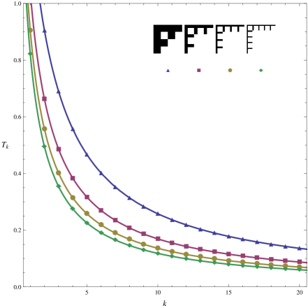
Figure 3: The critical temperature for the Sierpinski gaskets as a function of $k$. Convergence towards $T_{\infty}=0$ is very slow (logarithmic). The $k=3$ generators for (from left) the $L=2,3,4,5$ Sierpinski gaskets considered in the study are shown in the legend.

Even if $T_{\infty}=0$, it is interesting to infer from (19) the exact critical temperature for any finite $k$:

$$T_{k}=\frac{2}{\log\frac{1+\left(\!\sqrt{2}-1\right)^{1/L^{k}}}{1-\left(\!\sqrt{2}-1\right)^{1/L^{k}}}}\,.$$ (20)

This relation is instructive since it shows that convergence to the limiting value is very slow, more precisely logarithmic, as can be seen in Figure 3. It is interesting to look also at the correlation length, which from Eq. (9) turns out to be

$$\xi_{k}(v)=2\sqrt{\frac{v^{L^{k}}-v^{3L^{k}}}{\left(v^{L^{k}}\left(v^{L^{k}}+2\right)-1\right)^{2}}}\,.$$ (21)

This relation is visualised in Figure 4. The correlation length critical exponent is one, as in the one dimensional case, for all Sierpinski gaskets.

It is clear that a similar analysis, with similar conclusions, can be made for other families of fractals with finite ramification number. It is probably possible to obtain a closed formula for $P_{k}(v,\mathbf{k})$ for any fractal with this property. This is a clear indication of their triviality and effective one dimensional behaviour.

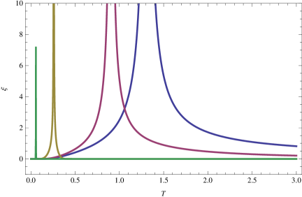
Figure 4: The correlation length $\xi_{k}$ for the $L=3$ Sierpinski gasket as a function of $T$ for the values $k=1,2,10,50$.

Analytical solution of the $k=1$ Sierpinski carpet.

We can give the analytical solution of the Sierpinski carpet $\rm{SC}(3,1)_{1}$. The critical temperature is the solution of

$$P_{\rm{SC}(3,1)_{1}}(v,0)=\Big{(}1-4v^{3}+5v^{4}-16v^{5}-10v^{6}-20v^{7}+v^{8}-24v^{9}+2v^{10}+v^{12}\Big{)}^{2}\,.$$ (22)

The only root in the range $0<v<1$ is $v_{c}=0.495968...$ which gives $T_{c}=1.83842...$ as reported in the $k=1$ entry of Table I. Note that it is a non-trivial fact and a consistency check that the 12^th degree polynomial in Eq. (22) has only one real solution in the physical range.

In this case we are also able to determine the full momentum dependence of the determinant

$$P_{\rm{SC}(3,1)_{1}}(v,\mathbf{k})=\qquad$$

$$\quad 1+10v^{4}+20v^{6}+119v^{8}+324v^{10}+876v^{12}+1284v^{14}+983v^{16}+412v^{18}+58v^{20}+8v^{22}+v^{24}$$

$$\quad-4v^{3}(1-v^{2})^{2}\Big{(}1+6v^{2}+21v^{4}+52v^{6}+69v^{8}+72v^{10}+29v^{12}+6v^{14}\Big{)}\Big{(}\!\cos 3k_{x}+\cos 3k_{y}\Big{)}$$

$$\quad-2v^{6}(1-v^{2})^{4}\left(7+18v^{2}+24v^{4}+14v^{6}+v^{8}\right)\Big{(}\!\cos 3(k_{x}+k_{y})+\cos 3(k_{x}-k_{y})\Big{)}$$

$$\quad+2v^{6}(1-v^{2})^{5}\left(1+4v^{2}+3v^{4}\right)\Big{(}\!\cos 6k_{x}+\cos 6k_{y}\Big{)}\,.$$ (23)

This relation clearly illustrates how non-trivial are the explicit solutions already at the level of the first iteration. It also shows how higher harmonics are excited, and that in $P_{\Lambda_{k}}(v,\mathbf{k})$ the coefficients of the trigonometric functions are polynomials in $v$. We have obtained similar relations for many $k=1$ non-trivial fractals, i.e. with infinite ramification number, while we have not been able to obtain closed analytical forms for the determinants as a function of $k$, and we suspect this to be a formidable task, even if not hopeless. Such a closed formula will constitute an explicit exact solution of the model.

Finally, we also report the correlation length in the $k=1$ case. Inserting Eq. (23) into Eq. (9) gives

$$\xi_{1}(v)=2\left(\frac{v^{3}\left(v^{2}-1\right)^{2}\left(v^{15}+12v^{14}+18v^{13}+58v^{12}-13v^{11}+144v^{10}-20v^{9}+138v^{8}+7v^{7}+104v^{6}+2v^{5}+42v^{4}+5v^{3}+12v^{2}+2\right)}{\left(v^{12}+2v^{10}-24v^{9}+v^{8}-20v^{7}-10v^{6}-16v^{5}+5v^{4}-4v^{3}+1\right)^{2}}\right)^{\frac{1}{2}}\,.$$

This correlation length diverges consistently at $v_{c}=0.495968...$ and when expressed in terms of the reduced temperature is plotted as the upper curve in Figure 9. Clearly $\nu=1$ as expected from universality.

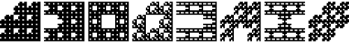
Figure 5: The $L=3$ Sierpinski carpet(s) considered in the study at their $k=4$ approximation.

III.3 Critical temperatures

Numerical analysis of critical temperatures.

We have reduced the calculation of the critical temperature on a lattice $\Lambda_{k}$ to finding the largest positive real eigenvalue $\lambda_{\Lambda_{k}}$ of the matrix $\mathbb{W}_{\Lambda_{k}}(0,0)$ corresponding to the weighted adjacency graph defined in the previous section. The $4L^{2k}\times 4L^{2k}$ matrix $\mathbb{W}_{\Lambda_{k}}$ is sparse, but its size grows rapidly as a function of the $k$. For $k>1$ we are not able to calculate analytically the eigenvalues but we instead resort to numerical calculations.

We use the shifted Arnoldi solver of Mathematica, which uses the ARPACK library and is sufficient for an initial proof of concept. The algorithm can be used to compute an arbitrary number of eigenvalues in the neighbourhood of a complex number, usually referred as the shift parameter. In our study, we compute the eigenvalue $\lambda_{\Lambda_{k}}$ using as a shift the eigenvalue $\lambda_{\Lambda_{k-1}}$.

A caveat of our approach is that it would give a wrong estimate of $\lambda_{\Lambda_{k}}$ if there was a complex eigenvalue with a small imaginary part in the neighborhood of $\lambda_{\Lambda_{k-1}}$. However, it turns out that the eigenvalue is isolated, as for instance illustrated in Figure 6 in the case of $\rm{SC}(3,1)_{3}$, for which we can compute the entire spectrum of the matrix $\mathbb{W}_{\rm{SC}(3,1)_{3}}(0,0)$. For larger $k$ we investigate the stability of our prediction depending on the value of the chosen shift parameter. For all the cases considered we observed that changing the shift leads to the same estimate of the critical temperature when we are able to compute enough eigenvalues. If we could not compute enough eigenvalues, then we find only non real eigenvalues. Therefore, in practice this numerical limitation does not arise.

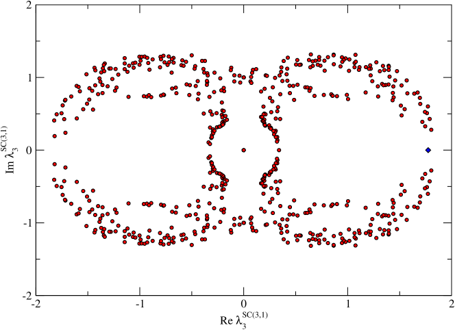
Figure 6: Eigenvalues of $\mathbb{W}_{\rm{SC}(3,1)_{3}}$. The only real eigenvalue larger than one is shown using a blue diamond.

Figure 7: Exact critical temperatures for the first seven approximands to the non-trivial $L=3$ Sierpinski carpets considered, together with a fit.

Generator	$d_{f}$	$k=1$	$k=2$	$k=3$	$k=4$	$k=5$	$k=6$	$k=7$
	$1.893$	$1.83842$	$1.67971$	$1.61601$	$1.58935$	$1.57798$	$1.57310$	$1.57099$
	$1.893$	$1.83842$	$1.66680$	$1.59188$	$1.55769$	$1.54140$	$1.53319$	$1.52872$
	$1.893$	$1.83842$	$1.65386$	$1.56759$	$1.52566$	$1.50446$	$1.49331$	$1.48719$
	$1.771$	$1.48866$	$1.18962$	$1.04440$	$0.965875$	$0.920115$	$0.892608$	$0.875999$
	$1.771$	$1.48866$	$1.18310$	$1.03567$	$0.955384$	$0.908286$	$0.879960$	$0.862996$
	$1.771$	$1.29944$	$0.983021$	$0.830078$	$0.739657$	$0.679436$	$0.636087$	$0.603146$
	$1.771$	$1.29944$	$0.97052$	$0.80394$	$0.699862$	$0.626109$	$0.569437$	$0.523428$
	$1.771$	$1.29944$	$0.958433$	$0.780739$	$0.667582$	$0.586519$	$0.524012$	$0.473526$

Table 1: Exact critical temperatures for the various iterations of the $L=3$ Sierpinski carpets. The fractals are ordered from the largest to the lowest critical temperature. Note that for $k=1$ different lattices have the same critical temperature, since at this level, there are exactly the same.

Using this procedure, we can calculate the critical temperature up to $k=7$, for the $L=3$ fractals. To achieve this, we need to find a specific eigenvalue of a $19~{}131~{}876\times 19~{}131~{}876$ matrix. The calculations are limited by the available memory. All the computations performed in this section have been achieved running Mathematica on a single node with 20 cores and 128GB of memory. Without further method improvements a machine with more memory would be needed to compute $T_{k}$ for $k>7$.

The results for the $L=3$ Sierpinski carpets are given in Table 1. They are illustrated for the 8 fractals considered in Figure 7. The fractals considered here have two different fractal dimensions. However they differ by there number of active bonds. The three fractals that have a dimension close to two show a much faster convergence than the others. As seen in the previous section, in the case of the Sierpinski gaskets, fractals can show a very slow convergence in the $k\to\infty$ limit. We thus see that, for the fractals considered, the smaller the fractal dimension, the slower is the pace of convergence. We do not attempt to perform any extrapolation to $k\to\infty$ since, in our set-up, we lack a scaling theory that governs this limit as the volume is already infinite for every $k$.

As mentioned earlier, the method can be easily applied to other fractals, and we investigate some of them with $L=4,5$ and $7$ as summarized in Table 2. The fractal $\widetilde{\rm{SC}}(7,3)$ is defined by removing nine distinct uniformly distributed cells as illustrated in Figure 8. The two fractals with $L=7$ generators considered here have the same fractal dimension but different lacunarity. They have been discuss in gefen:1980aa ; gefen:1984aa .

Fractal	$d_{f}$	$k=1$	$k=2$	$k=3$	$k=4$	$k=5$
$\rm{SC}(4,2)$	$1.792$	$1.62129$	$1.36891$	$1.25015$	$1.18451$	$1.14280$
$\rm{SC}(5,1)$	$1.975$	$2.11926$	$2.07899$	$2.06904$	$2.06672$	-
$\rm{SC}(5,3)$	$1.723$	$1.48748$	$1.19857$	$1.05787$	$0.97483$	-
$\rm{SC}(7,3)$	$1.896$	$1.92863$	$1.85117$	$1.8334$	$1.82927$	-
$\widetilde{\rm{SC}}(7,3)$	$1.896$	$1.57100$	$1.39728$	$1.34601$	$1.32719$	-

Table 2: Exact critical temperatures for the various Sierpinski carpets with $L>3$.

Comparison with Monte Carlo approach.

Defining $\Lambda_{k,l}\equiv{\rm sc}(L,b)_{k,l}$ as a finite lattice defined by an $l\times l$ array of ${\rm sc}(L,b)_{k}$ building blocks. Defining $T_{k,l}$ as the critical temperature of the lattice $\Lambda_{k,l}$, where obviously for a finite $l$ the critical temperature is defined for instance as the maximum of the specific heat. Usually Monte Carlo studies reports $T_{k,1}$ whereas we compute $T_{k,\infty}=\lim_{l\to\infty}T_{k,l}$. While $T_{k,l}$ depends on the lattice definition of the critical temperature, the value of $T_{k,\infty}$ is unique. The critical temperature of the fractal is approached in the limit of $k\to\infty$ in both cases. Since it is proven that for fractals with infinite ramification number $T_{\infty}>0$, the two approaches must yield to the same limiting value. The rate of convergence is a priori unknown in both cases.

In table 3 we compare our results for $T_{k,\infty}$ with the results for $T_{k,1}$ obtained using Monte Carlo simulations for various fractals. The lattice estimates of the critical temperature are in a good agreement with our results and almost always within the estimated errors. As expected from the previous considerations, the fractals with the highest fractal dimensions exhibit also a better agreement.

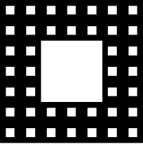
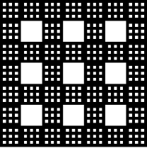
Figure 8: Generators $\rm{sc}(7,3)_{2}$ (left) and $\widetilde{\rm{sc}}(7,3)_{2}$ (right).

Authors	$T_{C}$	$\nu$	k
SC$\bf(3,1)\quad d_{f}=1.8927$
Bonnier et al. (1987) Bonnier:1987aa	$1.54$	$1.3$	$3$
Our work	$1.56759$	-	3
Pruessner et al. (2001) Pruessner:2001aa	$1.5266(11)$	$-$	$4$
Our work	$1.525660$	-	4
Pruessner et al. (2001) Pruessner:2001aa	$1.5081(12)$	$-$	$5$
Our work	$1.504460$	-	5
Pruessner et al. (2001) Pruessner:2001aa	$1.4992(11)$	$-$	$6$
Bab et al. (2005) Bab:2005aa	$1.4945(50)$	$\sim 1.39$	$6$
Our work	$1.493310$	-	6
Carmona et al. (1998) Carmona:1998aa	$1.481$	$1.70(1)$	7
Monceau et al. (1998) Monceau:1998aa	$1.482(15)$	$1.565(10)$	7
Our work	$1.48719$	-	7
Monceau et al. (2001) Monceau:2001aa	$1.4795(5)$	$>1.565$	8
SC$\bf(4,2)\quad d_{f}=1.7925$
Carmona et al. (1998) Carmona:1998aa	$1.077$	$3.23(8)$	6
Monceau et al. (2001) Monceau:2001aa	$<1.049$	$>3.37$	6
Our work	$1.1428$	-	5
SC$\bf(5,1)\quad d_{f}=1.9746$
Monceau et al. (2001) Monceau:2001aa	$2.0660(15)$	$1.083(3)$	5
Our work	$2.06672$	-	4
SC $\bf(5,3)\quad d_{f}=1.7227$
Monceau et al. (2001) Monceau:2001aa	$<0.808$	$>4.06$	5
Our work	$0.974828$	-	4
Ising $2d$	$2.269$	$1$	-

Table 3: Comparison with the literature (Monte Carlo study).

III.4 Correlation lengths

As explained in section II.2, we can also estimate the correlation length of the system as a function of $k$, $t=T/T_{C}-1$ (the reduced temperature) and $\Lambda_{k}$ using Eq. (9). We expect from universality that all approximands have $\nu=1$, since for finite $k$, they all belong to the universality class of the two dimensional Ising model. Different critical exponents for the fractal can emerge only in the limit $k\to\infty$ where the type of singularity manifested by the free energy at the critical point can change.

We checked numerically this expectation. Evaluating Eq. (9) exactly for various values of the reduced temperature, we computed the correlation length for various $L=3$ fractals with $k$ up to four. Our results for ${\rm SC}(3,1)_{k}$ are illustrated in Figure 9 where the correlation lengths have been normalized to exhibit universality. As can be seen all the curves are compatible with $\nu=1$, but the scaling region shrinks as $k$ increases. Our results for the normalized correlation lengths of all $L=3$ fractals considered in Table 3 are represented in Figure 10. This picture represents a strong confirmation of universality.

This analysis implies that if the limit $k\to\infty$ is continuous then the critical exponent $\nu$ is one for the fractals of dimension below two. In contrary, if the limit is discontinuous other values are possible, but our approach cannot determine them, unless we are able to calculate analytically the determinant $P_{\Lambda_{k}}(v,\bf{k})$ as we did for the Sierpinski gaskets. Without such an analytical formula, at any finite $k$, it is difficult to estimate the critical exponent $\nu$ of the fractals.

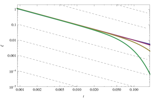
Figure 9: Normalized correlation lengths of the Sierpinski carpet starting from above for $k=1,2,3,4$ as a function of the reduced temperature $t$. As expected from universality all all curves tend to $t^{-1}$ for small enough $t$.

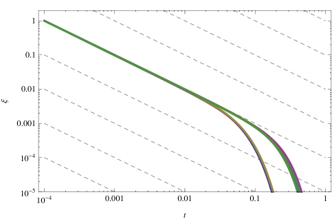
Figure 10: Universality strikes back: normalized correlation lengths of the non-trivial $L=3$ Sierpinski carpets for $k=4$ as a function of the reduced temperature $t$. As expected from universality all curves tend to $t^{-1}$ (dashed lines) for small enough $t$.

Comparison with the Monte Carlo approach.

Defining, in analogy with what done in the case of the critical temperatures, $\nu_{k,l}$ as the critical exponent for the $k^{th}$ iterations of systems of size $l$. We compute $\nu_{k,\infty}$, and find $\nu_{k,\infty}=1$ for all $k$ as expected from universality. For the fractal critical exponent $\nu_{\infty}=\lim_{k\to\infty}\nu_{k,l}$ to be different from one the limit has to be discontinuous. The standard theory of finite size scaling Fisher:1972zza applies to changing $l$ while keeping $k$ fixed, and this scaling should lead to $\lim_{l\to\infty}\nu_{k,l}=1$ as required by universality. This was already noted by Pruessner:2001aa . To our knowledge there is no scaling theory with respect to $k$ at fixed $l$, in particular for $l=1$, which is used in some Monte Carlo simulations. For $l=\infty$ there is not such theory because $\nu_{k,\infty}=1$ for all finite $k$. Hence, some Monte Carlo simulations rely on a possible scaling on $\nu_{k,1}$, which might not exist.

Furthermore, our results show that the scaling region where $\xi\sim t^{-1}$ shrinks as $k$ is increased, as shown in the Figure 9. This suggests that it becomes increasingly difficult to compute the critical exponent $\nu_{k,1}$ keeping $k$ fixed and calculating it using the reduced temperature as the scaling variable, which is an other approach used in Monte Carlo simulations.

As shown in the table 3, Monte Carlo simulations provide estimates for the critical exponents, in particular $\nu$. They report values of $\nu>1$ even bigger than four Monceau:2001aa . It might be that the lattice simulations are able to capture the right universal properties of the fractals. Nevertheless, a better theoretical understanding of the situation is needed.

IV Conclusions and Outlook

We showed that it is possible to approximate the solution of fractal Ising models via a sequence of exact solutions of Ising models on finite periodic representations of the fractal under consideration. We found that the rate of convergence to the exact solution can be very slow, as the explicit example of the exact solution of the Sierpinski gasket model shows. We found estimates for all $L=3$ fractals, and in particular for the Sierpinsky carpet. Numerical improvements can rapidly refine our results ultimately leading to the accurate determination of the exact critical temperatures for all non-trivial fractals of dimension smaller than two.

The problem is much more difficult in the case of the critical exponents since universality ultimately sets in and renders any finite periodic approximation useless to the scope. But we can still speculate on the actual values for the critical exponents of the fractals. Our analysis suggests two scenarios, related to the fate of the limits $\nu_{\infty}=\lim_{k\to\infty}\nu_{k,\infty}$ and $\alpha_{\infty}=\lim_{k\to\infty}\alpha_{k,\infty}$. Assuming the hyperscaling relation $\alpha=2-d_{f}\nu$ to hold true for fractals with infinite ramification number, then the continuity of the first limit implies $\nu_{\infty}=1$ and a change in the singularity structure of the free energy, i.e. $\alpha_{\infty}=2-d_{f}$. In this case both critical exponents will be continuous in the $d_{f}\to 1$ limit. If, instead, there is no change of singularity structure, i.e. $P_{\infty}(v,\bf{k})$ retains the polynomial zero it has in the finite $k$ cases, then $\alpha_{\infty}=0$ and, again assuming the hyperscaling relation, we find $\nu_{\infty}=2/d_{f}$, which is not continuous in the $d_{f}\to 1$ limit but is a fairly good approximation for all fractional dimensions as compared to the RG results Guida:1998bx ; Ballhausen:2003gx . Obviously, it can also be that both limits are discontinuous or that the hyperscaling relation is either violated or does not contain $d_{f}$. It can also be that these limits are sensible to the type of fractal under study, i.e they depend on fine details such as lacunarity or connectivity gefen:1980aa ; Monceau_2004 .

The question of the existence of a lower critical dimension, for fractals with infinite ramification number (or more restrictive properties), can now in principle be addressed by our method once the numerical routines are improved, since we have seen that the rate of convergence of the critical temperatures $T_{k}$ is slower the smaller the fractal dimension is. High values of $k$ will thus be needed to resolve the neighbourhood of a possible lower critical dimension.

Further interesting applications of our method are related to the study of Ising models on other non-translationally invariant lattices, like those defined on aperiodic or random lattices, or with random interactions.

Acknowledgments

We thank Rudy Arthur for initial participation and discussion. This work was supported by the Danish National Research Foundation DNRF:90 grant and by a Lundbeck Foundation Fellowship grant. The computing facilities were provided by the Danish Centre for Scientific Computing.

References

- (1) E. Ising, Z. Phys. 31, 253 (1925).
- (2) L. Onsager, Phys. Rev. (1944) 117.
-
(3)
Gefen Y, Aharony A and Mandelbrot BB
J. Phys. A 435 (1984);
Y. Higuchi and N. Yoshida J. Stat. Phys. 295 (1996);
R. Rammal J. Phys. (Paris) 191 (1984);
R.B. Stinchcombe Phys. Rev. B 2510 (1990). - (4) A Vezzani, J. Phys. A: Math. Gen. (2003) 1593.
- (5) M. Shinoda Journal of Applied Probability, Vol. 39, 1 (2002).
- (6) N. V. Vdovichenko, Sov. Phys. JETP (1965) 477-9.
- (7) R. P. Feynman, Statistical Mechanics, Benjamin/Cummings, Reading, MA, 1972.
- (8) A. Codello, J. Phys. A 43 (2010) 385002.
- (9) A. Codello, J. Phys. A 45, 465006 (2012) [arXiv:1204.3877 [hep-th]].
- (10) S. El-Showk, M. Paulos, D. Poland, S. Rychkov, D. Simmons-Duffin and A. Vichi, arXiv:1309.5089 [hep-th].
- (11) R. Guida and J. Zinn-Justin, J. Phys. A 31, 8103 (1998) [cond-mat/9803240].
- (12) H. Ballhausen, J. Berges and C. Wetterich, Phys. Lett. B 582, 144 (2004) [hep-th/0310213].
- (13) B. Bonnier, Y. Leroyer and C. Meyers Phys. Rev. B 37 5205 (1988).
- (14) Pai-Yi Hsiao and Pascal Monceau Phys. Rev. B 67 (2003), 064411.
- (15) Y. Gefen, B. B. Mandelbrot, and A. Aharony Phys. Rev. Lett. 45, 855 (1980).
- (16) D. Cassi Phys. Rev. Lett. 68, 3631 (1992).
-
(17)
Fàbio D. A. Aaräo Reis and R. Riera,
Phys. Rev. E 49, 2579 (1994);
B. Bonnier, Y. Leroyer, and C. Meyers, Phys. Rev. B 40, 8961 (1989). - (18) M. Kac and J. C. Ward, Phys. Rev. (1952) 1332.
- (19) S. Sherman, J. Math. Phys. 202 (1960).
- (20) T. Morita, J. Phys. A: Math. Gen. (1986) 1197-1205.
- (21) H.A. Kramers and G.H. Wannier, Phys. Rev. , (1941) 252.
- (22) R. Burioni, D. Cassi and L. Donetti, J. Phys. A: Math. Gen. 32 (1999) 5017–5027.
- (23) Y Gefen et al J. Phys. A: Math. Gen. 17 1277 (1984).
- (24) M. E. Fisher and M. N. Barber, Phys. Rev. Lett. 28, 1516 (1972).
- (25) G. Pruessner, D. Loison, and K. D. Schotte, Phys. Rev. B 64, 134414 (2001).
- (26) B. Bonnier, Y. Leroer and C. Meyers, J. Phys. (Paris) 48 533 (1987).
- (27) M. A. Bab, G. Fabricius, and E. V. Albano Phys. Rev. E 71, 036139 (2005).
- (28) José M. Carmona, Umberto Marini Bettolo Marconi, Juan J. Ruiz-Lorenzo, and Alfonso Tarancón Phys. Rev. B 58 , 14387 (1998).
- (29) Pascal Monceau and Michel Perreau, Phys. Rev. B 58 , 6386 (1998).
- (30) Pascal Monceau and Michel Perreau, Phys. Rev. B 63 (2001) 18, 184420.
- (31) Monceau, Pascal; Hsiao, Pai-Yi Physica A, Volume 331, Issue 1, 1-9.