eurm10 \checkfontmsam10 \pagerange119–126
A numerical investigation on active and passive scalars in isotropic compressible turbulence
Abstract
Using a simulated system of temperature and concentration advected by a turbulent velocity, we investigated the statistical differences between active and passive scalars in isotropic compressible turbulence, as well as the effect of compressibility on scalar transports. It shows that in the inertial range, the kinetic energy spectrum and scalar spectra follow the power law, and the values of the Kolmogorov and Obukhov-Corrsin constants are and , respectively. The appearance of plateau in the transfer flux spectrum confirms the balances between dissipations and driven forcings for both velocity and passive scalar. The local scaling exponent computed from the second-order structure function exists flat regions for velocity and active scalar, while that for passive scalar takes first a minimum of then a maximum of . It then shows that the mixed third-order structure function of velocity and passive scalar satisfies the Yaglom’s -law. For the scaling exponent of structure function, the one of velocity and passive scalar mixing is between those of velocity and passive scalar, while the one of velocity and active scalar mixing is below those of velocity and active scalar. At large amplitudes, the probability distribution function (p.d.f.) of active scalar fluctuations is super-Gaussian, whereas that of passive scalar fluctuations is sub-Gaussian. Moreover, the p.d.f.s of the two scalar increments are concave and convex shapes, respectively, which exhibit strong intermittency at small scales, and approach Gaussian as scale increases. For the visualization of scalar field, the active scalar has ”ramp-cliff” structures, while the passive scalar seems to be dominated by rarefaction and compression. By employing a ”coarse-graining” approach, we study scalar cascades. Unlike passive scalar, the cascade of active scalar is mainly determined by the viscous dissipation at small scales and the pressure-dilatation at large scales, where the latter is substantial in the vicinity of small-scale shocklets but is negligible after space averages, because of the cancelations between rarefaction and compression regions. Finally, in the inertial range, the p.d.f.s for the subgrid-scale fluxes of scalars can collapse to the same distribution, revealing the scale-invariant feature for the statistics of active and passive scalars.
keywords:
compressible turbulence, isotropic turbulence, active scalar, passive scalar, numerical simulation1 Introduction
Scalar mixing in turbulent flows includes generation of scalar fluctuations, distortion of scalar interfaces, and creation of intermittent scalar gradients at small scales. It is of fundamental importance in a variety of fields ranging from the scattering of interstellar mediums in Universe (Meyer et al., 1998; Cartledge et al., 2006), the dispersion of air pollutants in atmosphere (Lu & Turco, 1994, 1995), to the combustion of chemical reactions in engine (Pope, 1991; Warhaft, 2000). In the literature of fluid dynamics, scalar mixing is also called as ”scalar turbulence”, which has been extensively studied. It was Obukhov (1949) and Corrsin (1951) first applied the Kolmogorov theory to passive scalar advected by incompressible turbulence, and derived the power-law scaling of the second-order scalar increment structure function
| (1) |
where , and are the dissipation rates of energy and scalar, respectively. The sign denotes ensemble average. This result indicates that the cascade of passive scalar is similar to the classical energy cascade for velocity (Monin, 1975). In particular, the scalar fluctuations are generated at large scales and transported through successive breakdowns into smaller scales, the cascade proceeds until fluctuations are dissipated at the smallest scale. By this picture, an inertial-convective range is defined between the largest and smallest scales. Hereafter, we call it inertial range if there is no ambiguity. The scalar spectrum in the inertial range is then given by
| (2) |
where is the Obukhov-Corrsin (OC) constant and regarded to be universal. Sreenivasan (1996) concluded that , and the experiments of passive scalar in decaying grid turbulence by Mydlarski & Warhaft (1998), for varying from to , showed that . In numerical simulation, Wang et al. (1999) studied the refined similarity hypothesis for passive scalar and gave that at , and Yeung et al. (2002, 2005) found that in the scalar turbulence with mean gradient, was around in the range of .
Nevertheless, the Kolmogorov-Obukhov-Corrsin theory fails in describing the well-known anomalous scaling problem of passive scalar except for
| (3) |
It was Kraichnan (1994) first proposed a predictable model for the scaling exponent of passive scalar in white-noise turbulence, using a linear anstaz. Then, Shraiman & Siggia (1994) gave a series of white-noise equations for the structure functions of passive scalar. Although the approach of white-noise velocity is insightful and has provoked many theoretical and computational work, it is clear that a more realistic velocity either incompressible or compressible must be considered for the problem. Cao & Chen (1997) computed passive scalar in the Navier-Stokes (NS) turbulence and developed a bivariate log-Poisson model. Watanabe & Gotoh (2004) studied the statistics of passive scalar in homogeneous turbulence and found that in the inertial range, the passive scalar scaling follows the bivariate log-Poisson model.
The experimental measurements in decaying grid turbulence at high Peclet number (Mydlarski & Warhaft, 1998) showed that the p.d.f. of passive scalar is sub-Gaussian, which is identical to the simulation data from Wang et al. (1999), and Watanabe & Gotoh (2004). Further, the p.d.f. of passive scalar increment deviates distinctly from Gaussian at small scales and approaches Gaussian when scale increases. At large amplitudes, the p.d.f. tail of passive scalar is convex, whereas that of velocity increment is concave. The passive scalar field has the so-called ”ramp-cliff” structures (Chen & Kraichnan, 1998; Watanabe & Gotoh, 2004), which are produced by stretching and shearing of vortices. Specially, turbulent mixing effectively throws out high gradient events, forming the large-scale ramp structures of low gradient which are reconciled with the existing small-scale cliff structures of high gradient (Shraiman & Siggia, 2000). Thus, scalar dissipation is small in ramps but is large in cliffs.
When the Schmidt number is , the scalar fluctuations are dissipated at the so-called Batchelor scale . Batchelor (Batchelor, 1959) predicted that in the viscous-convective range (i.e. ), the scalar spectrum obeys a power law, which has been confirmed by many simulations such as Yeung et al. (2002, 2004), Antonia & Orlandi (2003), and Donzis et al. (2010). On the contrary, when , the scalar fluctuations decay strongly at the OC scale . Standard arguments by Batchelor, Howells and Townsend showed that when the Reynolds number is sufficiently high, the scalar spectrum follows a power law in the inertial-diffusive range (i.e. ). Recently, this conclusion has been proved by Yeung & Sreenivasan (2012, 2014).
The current understanding of scalar transport in compressible turbulence lags far behind the knowledge accumulated on the incompressible one. Previous studies involved the cascade of passive scalar in compressible turbulent flows were focused on the dependence of passive scalar trajectory on the degree of compressibility (Chertkov et al., 1997, 1998). It was analyzed by Gawedzki & Vergassola (2000) that for weak compressibility, the direct cascade of passive scalar associating with the explosion of initially close trajectories takes place, which is similar to that occurs in incompressible turbulence. By contrast, when compressibility is strong enough, the passive scalar trajectories collapse, and there arise the excitation of nonintermittent inverse cascade at large scales and the suppression of dissipation at small scales. Celani et al. (1999) studied the dynamical role of compressibility in the intermittency of passive scalar for the direct cascade regime, and pointed out that due to the slowing down of Lagrangian trajectory separations, the reinforced intermittency would appear for increasing compressibility. Recently, Ni & Chen (2012) performed simulations of passive scalar in one-dimensional (1D) compressible NS turbulence, and observed that starting from certain medium scales, the transfer flux of passive scalar transports upscale. Nevertheless, so far there is no observation for the inverse cascade of passive scalar in three-dimensional (3D) compressible turbulent flows, even the value of turbulent Mach number reaches at (Pan & Scannapieco, 2011). Furthermore, it was found that the passive scalar scaling in supersonic turbulence computed from the piecewise-parabolic method (PPM) simulation accords well with the SL94 model (She & Leveque, 1994). At low , the field structure of passive scalar is similar to that in incompressible turbulence, while at high , it is primarily dominated by large-scale rarefaction and compression (Pan & Scannapieco, 2010).
Contrasting to passive scalar, an active scalar always provides an impact on velocity by way of an extra term, i.e. buoyancy, added to the velocity equation, resulting in a two-way coupling between the velocity and scalar fields. Thus, it belongs to nonlinear problems. Celani et al. (2002a, b, 2004) studied the university and scaling of active and passive scalars by simulating four different numerical systems, and obtained the results that when the statistical correlation between active scalar forcing and advecting velocity is sufficiently weak, the active and passive scalars share the same statistics; however, when the statistical correlation is strong, the two scalars behave quite different. In the context of shell model, Ching et al. (2003) argued that the different scaling behaviors are attributed to the fact of the active scalar equation possesses additional conservation laws, while in the passive scalar equation the zero mode problem is a secondary factor. In the thermal convection experiment, Zhou & Xia (2002) showed that the active and passive scalars share some similar statistical properties, such as the saturation of scaling exponent and the log-normal distribution of front width.
In this paper, we regard the temperature advected by a compressible turbulent velocity as an active scalar. Without an additional term to the velocity equation, the temperature brings substantially nonlinear feedback to the velocity through the way of density fluctuations, which fits the general spirit of active scalar. We carry out a numerical investigation on the turbulent temperature and concentration transports. Our attention is focused on the statistical differences between active and passive scalars, as well as the effect of compressibility on scalar fields. The system is simulated on a grid using a novel hybrid method. This method utilizes a seventh-order weighted essentially non-oscillatory (WENO) scheme (Balsara & Shu, 2000) in shock region and an eighth-order compact central finite difference (CCFD) scheme (Lele, 1992) in smooth region outside shock. In addition, a new numerical hyperviscosity formulation is proposed to improve the numerical instability in simulation without compromising the accuracy of the method. As a result, the hybrid method has spectral-like spatial resolution in computing highly compressible turbulence. In comparison, though the PPM method can simulate compressible flows at higher turbulent Mach number, the absence of viscous dissipation brings a series of unphysical problems. The details of the hybrid method has been described in Wang et al. (2010). We hope that our comprehensive study will advance one’s understanding of the statistics of active and passive scalars in the small-scale compressible turbulence.
The remainder of this paper is organized as follows. The governing equations and basic parameters, along with the computational method, are described in Section 2. The fundamental statistics of the simulated system is provided in Section 3. The probability distribution function and structure function scaling are analyzed in Section 4. In Section 5, we describe the statistical behaviors of field structures. The discussions on the cascades of active and passive scalars are given in Section 6. Finally, we give the summary and conclusions in Section 7.
2 Governing equations, simulation parameters and methods
We consider a dynamic system of temperature and concentration transports by a turbulent velocity field under the idea gas state. The system is driven and maintained in a stationary state by the large-scale velocity and passive scalar forcings. Similar to Samtaney et al. (2001), we shall introduce a set of reference scales to normalize the hydrodynamic and thermodynamic variables. Since these variables together contain five elemental dimensions, we first introduce five basic reference scales as follows: for length, for density, for velocity, for temperature, and for concentration. Then we obtain the reference sound speed , kinetic energy per unit volume , pressure , and Mach number , where is the specific heat ratio, is the specific gas constant, and and are the specific heats at constant pressure and volume, respectively. By adding a reference dynamical viscosity , thermal conductivity , and molecular diffusivity , we derive three additional basic parameters including the reference Reynolds number , Prandtl number , and Schmidt number . In our simulation, the values of , and are set as , and , respectively. Then the flow system is completely determined by the two parameters of and .
Based on the above reference scales, the dimensionless form of the governing equations for the simulated system are written as
| (4) | |||
| (5) | |||
| (6) | |||
| (7) | |||
| (8) |
where and . The primary variables are the density , velocity , pressure , temperature , and concentration . is the large-scale velocity forcing, where is the Fourier amplitude and is perpendicular to the wavenumber vector (Ni & Chen, 2012; Ni et al., 2013). Similarly, the large-scale passive scalar forcing is , and the Fourier amplitude is also perpendicular to the wavenumber vector (Ni & Chen, 2012). The inclusion of the large-scale cooling function in the energy equation is to remove the accumulated internal energy at small scales, and its detail can be found in Wang et al. (2010). The viscous stress and total energy per unit volume are defined by
| (9) |
| (10) |
where is the dilatation, a flow variable that measures the local rate of expansion or compression. Here the dimensionless dynamical viscosity , thermal conductivity and molecular diffusivity are considered to vary with temperature through the Sutherland’s law (Sutherland, 1992) as follows
| (11) |
The system is solved numerically in a cubic box with periodic boundary conditions, by adopting a new computational approach (Wang et al., 2010). To obtain statistical averages of interested variables, a total of eighteen flow fields spanning the time period of were used, where is the large-eddy turnover time, and the system achieves the stationary state at the time of . Instead of the reference Mach number and Reynolds number , in simulation the flow is directly governed by the turbulent Mach number and Taylor microscale Reynolds number (Samtaney et al., 2001)
| (12) |
| (13) |
where is the r.m.s. magnitude of velocity, and is the Taylor microscale, which is defined as
| (14) |
In our simulation, by setting and , we obtained the time-average values of and . Although there is hardly a real instance with such values of and , the investigation reveals certain universal features of inertial ranges for compressible flows at different Reynolds numbers.
3 Fundamental statistics of simulated system
Table 1 lists some overall statistics of the velocity field. The resolution parameter is , where and are the largest solved wavenumber and the Kolmogorov scale , and their values are and , respectively. The integral scale is computed by
| (15) |
where is the kinetic energy spectrum per unit mass, namely,
| (16) |
The ratio is , representing the range of scales in the velocity field. The r.m.s. magnitudes of dilatation and vorticity are computed by , , with respective values of and . Then the ratio is , indicating that the compressibile effect makes a significant contribution to the statistics of velocity gradient tensor. This character is further demonstrated by the ensemble average of the velocity derivative skewness, which is defined by
| (17) |
The value of is equal to , much greater than typical values of observed in incompressible turbulence (Ishihara et al., 2007). This deviation is mainly caused by the presence of the small-scale shocklets in compressible turbulence.
| Scalar | ||||||||
|---|---|---|---|---|---|---|---|---|
| Te | ||||||||
| Co |
As for the scalar fields, their overall statistics are summarized in Table 2. The effective resolution parameters are for temperature and for concentration. The integral scale for scalar is computed by
| (18) |
Hereafter is denoted as or whenever there is no special illustration. is the scalar spectrum per unit mass, and its definition is similar to Equation (3.2). is the r.m.s. magnitude of scalar. The ratio for temperature and concentration are and , respectively. It shows that the ranges of scales for the two scalars are smaller than that for the velocity. Furthermore, the ensemble average of the skewness of scalar derivative is defined by
| (19) |
The values of are for temperature and for concentration, significantly smaller than in magnitude. Besides, the Taylor microscale , defined similarly to , are for temperature and for concentration.
The application of Helmhotlz decomposition (Erlebacher & Sarkar, 1993) to velocity field gives that
| (20) |
where is the solenoidal component and satisfies , and is the compressive component and satisfies , and is the Levi-Civita symbol. In Table 1, we compile the relevant statistics associated with the solenoidal and compressive processes. The r.m.s. magnitudes of solenoidal and compressive velocity are and . This leads the ratio of to be . We also note that is larger than , indicating that the compressible effect plays a more significant role at the small scales. The r.m.s. magnitudes of scalars presented in Table 2 are and .
Let us now focus the governing equation of the kinetic energy . According to Andreopoulos et al. (2000), it can be written as follows
| (21) |
where is the material derivative. On the right-hand side (R.H.S.) of Equation (3.7), the viscous dissipation rate is divided into three parts: the solenoidal dissipation rate , the dilatation dissipation rate , and the mixed dissipation rate , which represents the contribution to dissipation rate from the non-homogeneous component of compressible flow, and is zero in the incompressible limit. We find that and , meaning that the mixed part gives a negative contribution to the viscous dissipation rate. The ratio is , close to the estimated value of , where /2 and . In addition, the ensemble-average value of the injected energy is , implying that there is a main balance between the velocity forcing and viscous dissipation. As long as the velocity and temperature fields are statistically stationary, one must have .
By Equations (2.2)-(2.3), we derive the governing equation of temperature as follows
| (22) |
where is the Peclet number. The dissipation rates of temperature and concentration are defined by
| (23) |
| (24) |
It shows in Table 2 that and are and , respectively, and is . This confirms the approximative balance between the passive scalar forcing and molecular dissipation. The values of the temperature and concentration variances per unit volume are and , where and .
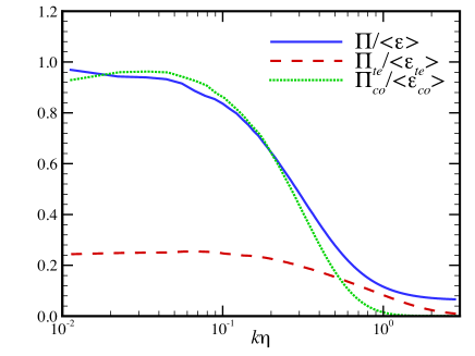
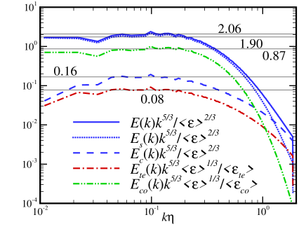
Figure 1 shows the compensated spectra of the kinetic energy and its two components and , as well as those of the scalars and . The inertial ranges of these spectra are clearly identified in the range of . We observe that the Kolmogorov constant of and OC constants of and read from the spectra are
| (25) |
Here is slightly higher than the typical values observed in incompressible turbulent flows (Wang et al., 1996), and is in well agreement with that from passive scalar in incompressible turbulence provided by Wang et al. (1999). However, is roughly one order of magnitude smaller than . The reason is due to the fact that the transfer flux of active scalar is more tightly associated with the compressive component of velocity, which contributes a small fraction to the kinetic energy. The spectra of kinetic energy and its solenoidal component almost overlap, except at high wavenumbers where the compressive component dominates the energy content. Furthermore, for the compressive component, the compensated energy level in the inertial range is roughly one order of magnitude smaller, but decays more slowly in the dissipative range. For scalars, the concentration spectrum is close to the kinetic energy spectrum and its solenoidal component, while the temperature spectrum resembles the compressive component.
Similar to Watanabe & Gotoh (2004, 2007), we define the transfer functions of the kinetic energy and scalars in wavenumber space as follows
| (26) | |||
| (27) |
where and are the terms of the velocity and passive scalar forcings in wavenumber space. Then the transfer fluxes of the kinetic energy and scalars across the wavenumber are
| (28) |
In Figure 2 we plot the spectra of transfer fluxes for the kinetic energy and scalars against the dimensionless wavenumber , normalizing by their ensemble averages of dissipation rates. It is found that and are close to unity in the ranges of and , respectively, over which and are in the inertial range and thus have the power law. By contrast, in the range of , is only of . This indicates that the dominance of the rarefaction and compression motions leads the flux transfer of temperature to being not follow the Kolmogorov picture. The shift towards higher wavenumbers is due to that the OC scale of temperature is larger than the Kolmogorov scale. Furthermore, the constancy of the transfer-flux spectra in certain wavenumber ranges indicate that the velocity and scalar fields are really in the equilibrium states.
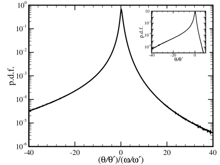
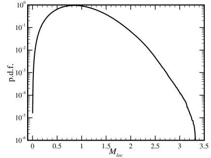
The p.d.f. of the ratio of the normalized dilatation to vorticity magnitude is shown in Figure 3. The p.d.f. is negatively skewed, exhibiting that the events of large negative ratio is substantial, even though has a small value of . Similar to those of dilatation, the p.d.f. tails of the ratio are concave. In the inset we plot the p.d.f. of the normalized dilatation with strongly negative skewness. This feature has already been observed in weakly and moderately compressible turbulent flows (Porter et al., 2002; Pirozzoli & Grasso, 2004). It was claimed by Pirozzoli & Grasso (2004) that the p.d.f. becomes more skewed towards the negative side as the turbulent Mach number increases. This point has been confirmed in our simulation. In Figure 4 we plot the p.d.f. of the local Mach number . Clearly, a substantial portion of the velocity field is supersonic, where the maximum of is . The p.d.f. peaks at . It reveals that in compressible turbulence, the small-scale shocklets generated by velocity fluctuations distribute randomly at different scales.
The structure functions of the longitudinal velocity increment , and the scalar increment are defined by
| (29) |
where is the separation distance between two points and is the order number. The Kolmogorov theory predicts that the structure functions scale as . In Figure 5 we plot the second-order structure functions of , and against the normalized separation distance . It shows that for and , the regions corresponding to the flat local scaling exponents are observed in the range of . By contrast, for , in the same range there are two different regions, in which the local scaling exponent takes first a minimum and then a maximum, and crossover occurs in the range of . Further, we plot the mixed second-order structure functions of velocity and scalars, with the relevant definition as follows
| (30) |
It shows that the behaviors of and are similar to those of and , namely, for the local scaling exponents, there are neither local minima nor local maxima. Thus, we speculate that throughout the range of , the transfer functions of both temperature and concentration at a given order number have single scaling exponents.
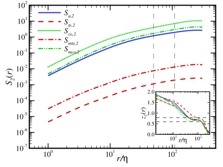
In the inset we plot the local scaling exponents as functions of , defining as
| (31) |
| (32) |
In the range of , and are almost constant and have the around values of and , respectively. For and , their constant values of and are found in the ranges of and , respectively. In terms of , it first decreases from small scales, and achieves a local minimum of at , then quickly increases and reaches a local maximum of at , after that, decreases again. To some extent, the behaviors of the second-order structure functions and their local scaling exponents in this study are similar to those observed in the 1D compressible turbulence (Ni & Chen, 2012). However, so far there are still unclear in two aspects: (1) whether a flat region in appears at the level of the local minimum or maximum as the Reynolds number increases; and (2) whether the local minimum and maximum features of disappears when the Schmidt number .
In the final of this section, we focus our attention on the applicability of the Kolmogorov’s and Yaglom’s -laws to compressible turbulence. The Kolmogorov’s -law is an asymptotically exact result for incompressible turbulent flows, and can be obtained from the Karman-Howarth equation (Pope, 2000). When the Reynolds number is sufficiently high, the velocity field of a stationary incompressible turbulence obeys the following equation
| (33) |
In the range of , the second and third terms on the R.H.S. of Equation (3.19) vanish, and then it yields to the -law
| (34) |
Similarly, the Yaglom’s -law is the asymptotically exact result for incompressible scalar turbulence, and was derived by Yaglom in (Yaglom, 1949). It reads as
| (35) |
where denotes the molecular diffusivity. When , Equation (3.21) is reduced to the -law
| (36) |
It should be pointed out that the smallest scale for the -law to hold is rather than . In this study the Batchelor scales for temperature and concentration are and , respectively.

In Figure 6 we plot the third-order velocity structure function and the mixed third-order velocity-scalar structure functions and , against the normalized separation distance . For and , there are plateaus in the ranges of and , respectively. Contrarily, there is no clear plateau observed in . Instead, it peaks at the around value of , sharing a similar explanation with the spectrum of temperature transfer flux. The inset shows the details of flat regions for . The level values computed from the plateaus are and , which are very close to and , respectively. This concludes that the velocity and passive scalar in our simulation satisfy the exact relations of structure functions derived from incompressible flows.
4 Probability distribution function and high-order statistics
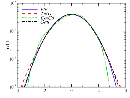
As we known, the intermittency in turbulence can be characterized by the behaviors of the p.d.f. tails of velocity and scalar increments. Figure 7 shows the time-average one-point p.d.f.s of the normalized fluctuation components of velocity, temperature and concentration, where , and have been referred in Section 3. The p.d.f. with Gaussian distribution is plotted for comparison. We find that at small amplitudes, the p.d.f.s of velocity and temperature are very close to Gaussian, while that of concentration occurs small oscillations. The reason is that in turbulence the fluctuations of concentration are usually more intense than those of velocity and temperature. At large amplitudes, the p.d.f. of temperature decays smoothly and more slowly than Gaussian, and thus is called as super-Gaussian. This feature is also found from the scalar in 3D Kraichnan-model flows (Balkovsky & Lebedev, 1998; Mydlarski & Warhaft, 1998; Shraiman & Siggia, 2000; Celani et al., 2002a, b, 2004). By contrast, the p.d.f.s of velocity and concentration are called as sub-Gaussian, because they decay smoothly and more quickly than Gaussian, similar to the passive scalar in incompressible turbulence (Mydlarski & Warhaft, 1998; Watanabe & Gotoh, 2004).
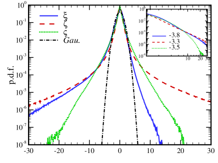
The time-average one-point p.d.f.s of the normalized longitudinal gradients of velocity, temperature and concentration are shown in Figure 8, where , and . It shows that the three p.d.f.s all deviate drastically from Gaussian (dash-dotted line), exhibiting strong intermittency. The p.d.f. of is negatively skewed, while those of and are approximately symmetric. In the negative gradient regions, the p.d.f. tails of and are longest and shortest, implying strongest and weakest in intermittency, respectively. However, in the positive gradient regions, the relative intensity of intermittency between and reverses. Furthermore, in the vicinity of varnishing gradient, the p.d.f.s of and peak higher than that of . In the inset we present the log-log plot of the large negative gradients versus their p.d.f.s. It shows that for , and , the values of the power-law exponents are , and , respectively. The major contributions of these p.d.f. tails are caused by small-scale shocklets rather than large-scale shock waves. Here we notice that the exponent value of for the p.d.f. of is a bit larger than that for the p.d.f. of velocity gradient, i.e. , in Burgers turbulence (E & Eijnden, 1999, 2000; Bec et al., 2000), but is substantially larger than that for the p.d.f. of dilatation, i.e. , in compressible turbulence (Wang et al., 2012a).
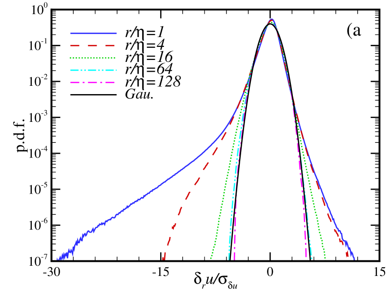
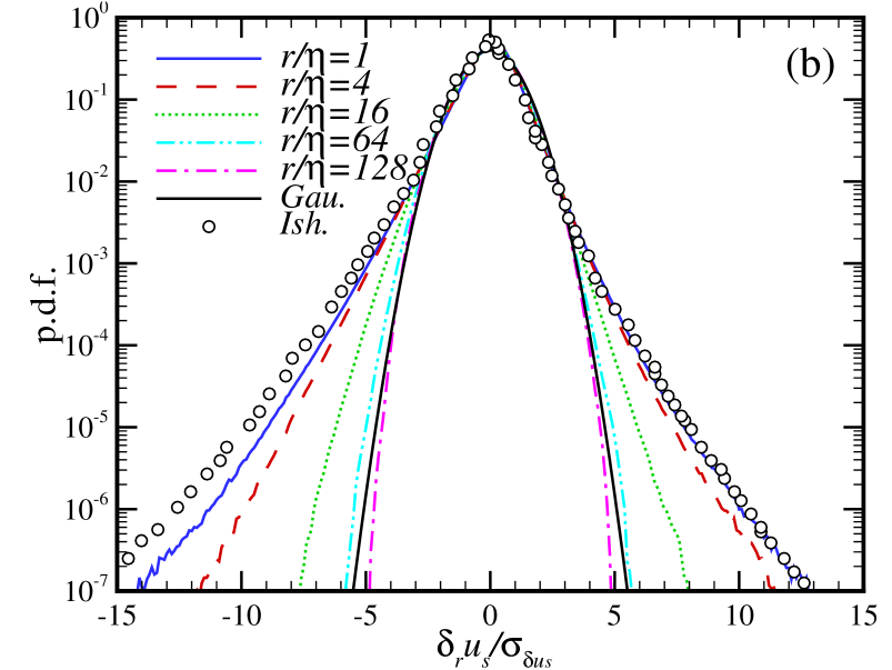
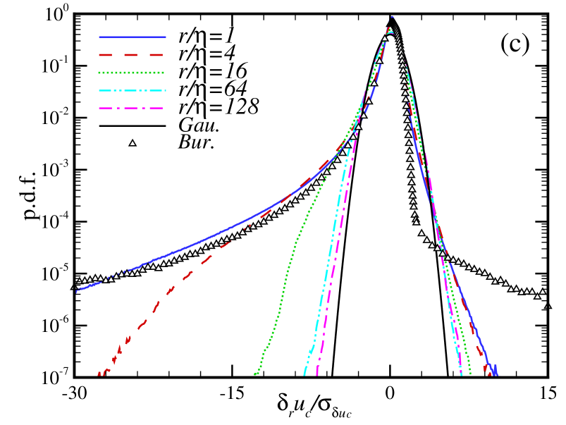
In Figure 9 we plot the p.d.f.s of the normalized longitudinal velocity increment and its components and , at the normalized separation distances of , , , and , where , and are the standard deviations of , and , respectively. We find that in Figure 9(a) at small scales (i.e. ), the left p.d.f. tail of is much longer than the right one, indicating strongly negative skewness. This feature is similar to the p.d.f. of longitudinal velocity gradient shown in Figure 8. The p.d.f. of gets more narrow and symmetric as increases, and it recovers to Gaussian without intermittency at . At large amplitudes, the p.d.f. tails are concave, which is in agreement with those observed in the experiments and simulations of incompressible turbulence. As for the solenoidal component shown in Figure 9(b), at small scales, on each side, the p.d.f. tails are slightly negative asymmetry and longer than Gaussian. When increases, they quickly become Gaussian. We notice that at , the p.d.f. of is close to that of provided by Ishihara et al. (2009) (circles), implying that the dynamics of solenoidal-component velocity is similar to that of velocity in incompressible turbulent flows. On the other side, the p.d.f. of the compressive component shown in Figure 9(c) displays strong intermittency at small scales, and thus, is like that of in Burgers turbulence (deltas). As increases, it approaches Gaussian as well. Besides, at large amplitudes the p.d.f. tails of the velocity component increments are also in concave shape.
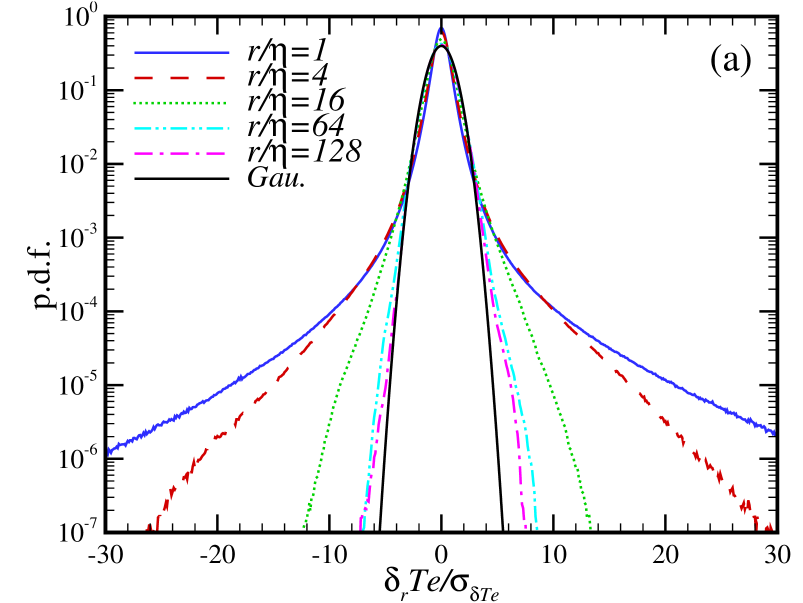
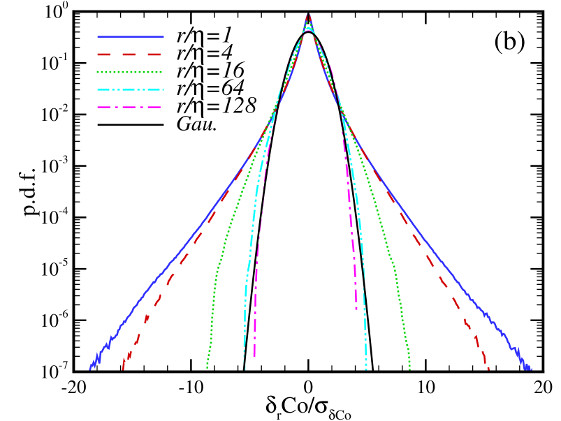
The p.d.f.s of the normalized scalar increments of and are shown in Figure 10, where and are the standard deviations of and , respectively. Obviously, these p.d.f.s are almost symmetric, even at small scales such as . When increases, they get narrower and approach Gaussian. It shows that on both sides the p.d.f. tails of are significantly longer than those of , indicating that in intermittency is much more intense than . Furthermore, at large amplitudes, the p.d.f. tails of temperature increment are concave, similar to those of longitudinal velocity increment, while those of concentration increment are convex. This feature has been found in the previous simulations of passive scalar advected by incompressible turbulence (Watanabe & Gotoh, 2004).
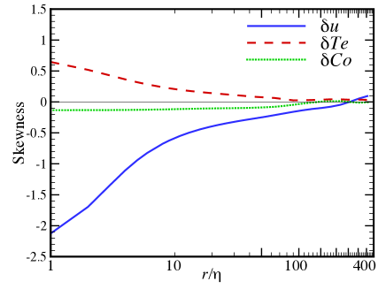
The change of the distributions of velocity and scalar increments can be characterized by their skewness and flatness as well. Those for the longitudinal velocity increment and scalar increment are defined as follows (Watanabe & Gotoh, 2004)
| (37) |
| (38) |
In Figure 11 we plot the skewness of , and against the normalized separation distance . It shows that in a wide scale range, and are negative and their local minima are around and , respectively, whereas is positive and its local maximum is around . As increases, the magnitudes of skewness fall and approach zero. We find that the Gaussianities of , and begin to appear even the scale is not very large. Throughout scale ranges, the magnitude of is always smaller than that of , implying a weaker degree of Gaussian departure.
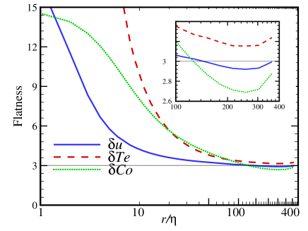
The flatness of , and against the normalized separation distance is plotted in Figure 12. It shows that when decreases, the three flatness all increase from the Gaussian value of , meaning that the intermittency of the flow increments emerge and enhance. In a wide scale range, is smallest, and thus, is weakest in intermittency. Compared to , is larger at small and moderate scales. However, the relation reverses in the range of , indicating that the intermittency of surpasses that of . This behavior has not been announced in the text of probability distribution function. The detailed variations of flatness in the range of are shown in the inset. At sufficiently large scales, and are below and thus are sub-Gaussian, while is above and thus are super-Gaussian. This feature is consistent with the behaviors of the p.d.f.s of fluctuations at large amplitudes shown in Figure 7.
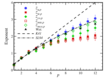
In Figure 13 we plot the scaling exponents of the structure functions of velocity and scalar increments as well as the mixed structure functions of velocity-scalar increments, as functions of the order number . These scalings are computed by taking averages on the local scaling exponents, where the curves are in the flat regions with finite widths. It shows that at large order numbers, , indicating that the velocity and temperature fields are weakest and strongest in intermittency, respectively. As for the mixed scaling, we obverse that locates between and , similar to that in incompressible turbulence. Nevertheless, it is interesting to find that locates below and . This phenomenon was previously appeared in 3D weakly compressible turbulence (Benzi et al., 2008) and 1D compressible turbulence (Ni & Chen, 2012). For comparison, we plot the velocity scaling given by the K41 (Kolmogorov, 1941) and SL94 (She & Leveque, 1994) models, and the passive scalar scaling provided by Watanabe & Gotoh (2004). Obviously, is close to the SL94 model and is smaller than Watanabe’s result. In our simulation, there is no saturation observed for the scalings of temperature and mixed velocity-temperature. Here we point out that the above results are obtained by using long-time averages (eighteen large-eddy turnover time periods). In fact, for each single time frame, the oscillation intensity of passive scalar scaling is much larger than those of passive scalar and velocity scalings.
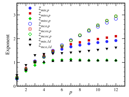
The Helmholtz decomposition on the mixed velocity-scalar scalings are depicted in Figure 14. It shows that and its two components and are almost identical, and locate far away from . By contrast, is a bit smaller than its solenoidal component , and the compressive component nearly collapses onto . This indicates that the scaling for the compressive component of the mixed velocity-temperature is similar to the Burgers scaling, which saturates at order number .
5 Behaviors of scalar field structures
So far we have focused on quantifying the fundamental statistics, probability distribution function and high-order statistics. In this section, we shall explore the flow structures. We hope that the structural analysis will complement the statistical results and provide a better understanding of the active and passive scalars in compressible turbulence.
5.1 Field structure
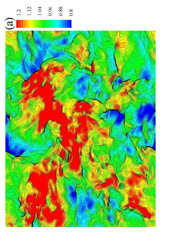
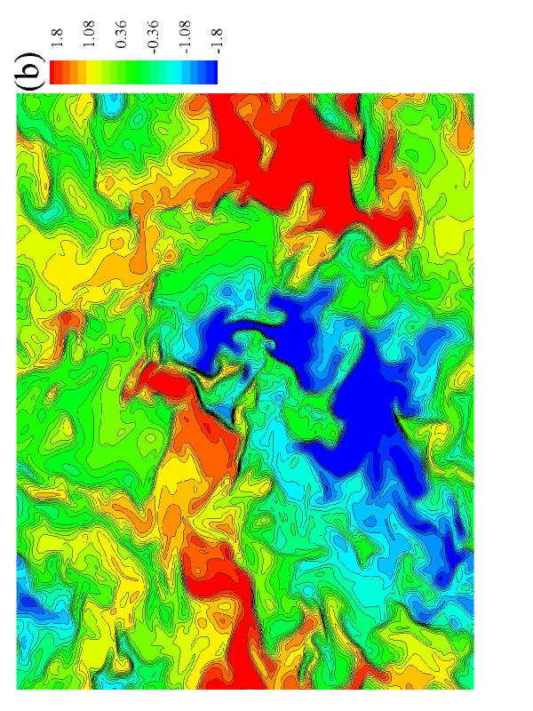
In Figure 15 we plot the two-dimensional slices (x-y plane) through the active and passive scalar fields simultaneously in the position of . The temperature field is depicted in the left panel, it shows that the small-scale ”cliff” structures are separated by the large-scale ”ramp” structures. The temperature fluctuations are small in the divided structure regions, however, they quickly increase when across the interfaces between cliffs and ramps. To some extent, this picture is similar to passive scalar in incompressible turbulence producing by stretching (Shraiman & Siggia, 2000), which rearranges scalar gradients and brings fluid elements with very different scalar level next to each other. By contrast, the concentration field shown in the right panel displays to be quite different. The concentration fluctuations seem to be dominated by the motions of rarefaction and compression, causing by shock fronts. Compared with the PPM simulations provided by Pan & Scannapieco (2010), the concentration field in this study is similar to that in the flow, showing the effect of shock waves. Nevertheless, we will show in the following section that the cascade of passive scalar is indeed mainly governed by the stretching of turbulence.
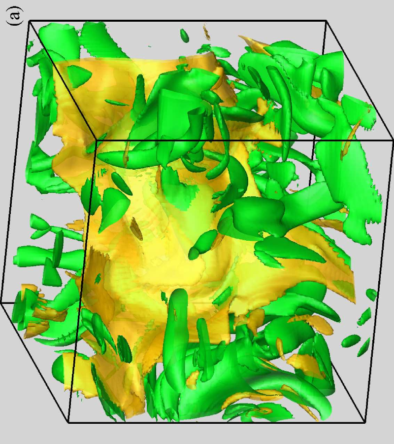
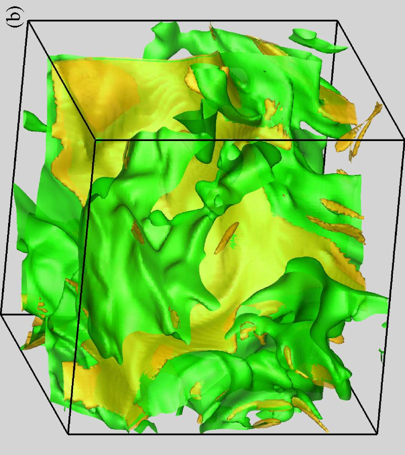
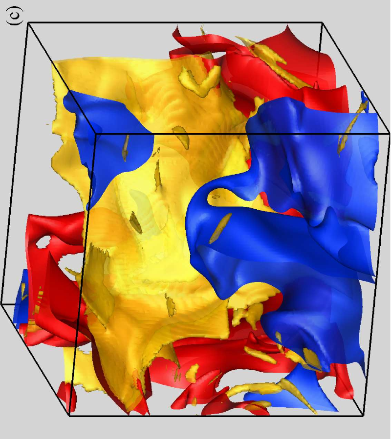
In Figure 16, the 3D isosurfaces of the magnitudes of dilatation , vorticity , temperature , concentration are displayed in a same subdomain (i.e. of the full domain). These isosurfaces are colored based on the local r.m.s. magnitudes, where the yellow isosurfaces stand for the large-scale shock wave with a thickness typically much smaller than the inertial scales, surrounding by the small-scale shocklets. In Figure 16(a), the green isosurfaces are the vortices under random distribution. When moving away from the shock wave, the geometric shape of vortices changes from sheetlike to tubelike. In Figure 16(b), the green sheetlike isosurfaces are temperature, exhibiting as wrinkled curves around shock wave. We notice that the surfaces of dilatation and temperature intersect with each other in certain positions. The isosurfaces of the positive and negative r.m.s. magnitudes of concentration are depicted in Figure 16(c) by the colors of blue and red, respectively. It shows that the concentration surfaces are sheetlike as well, and the curve surfaces of oppositive sign basically appears on each side of the shock front.
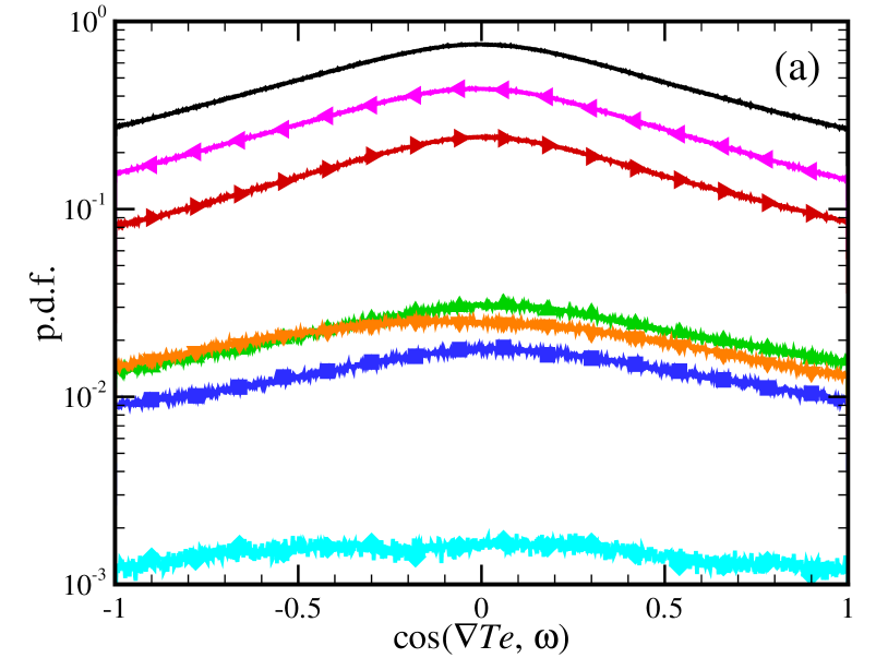
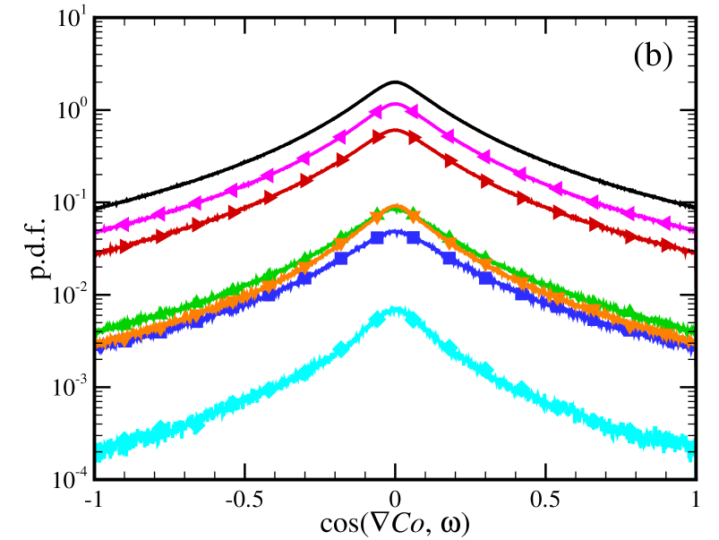
The p.d.f.s and conditional p.d.f.s of cosines of angles between vorticity and scalar gradients are shown in Figure 17. Unlike the positive alignments between vorticity and vortex stretching vector in turbulent flows (Kholmyansky et al., 2001; Wang et al., 2012b), the scalar gradients prefer to be perpendicular to the vorticity. In other words, the p.d.f.s get their maximal values in the vicinity of the angle. For each dilatation range, the p.d.f. and conditional p.d.f.s of concentration are much steeper than those of temperature, implying that the surfaces of passive scalar and vorticity are probably tangent to each other. In addition, we find that the p.d.f.s of the two scalars conditioned at each diltation level have similar relative relations.
5.2 Dissipation field structure
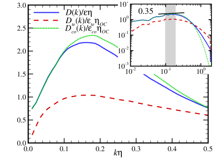
The normalized dissipation spectra of kinetic energy and scalars are plotted in Figure 18. The maximum dissipation spectrum of kinetic energy is about and occurs at , while that of concentration is about and occurs at . It indicates that the effectively smallest scale for concentration dissipation is around , a bit smaller than the Kolmogorov scale. The position for the maximum dissipation spectrum of temperature is , though the related OC scale is . So far the behind reason is unclear. In the inset we present the log-log plot. It shows that in the inertial range of , the slope values of the dissipation spectra are about , close to . In inertial range the spectra of kinetic energy and scalars follow the power law, therefore, the power law of the corresponding dissipation spectra should be .
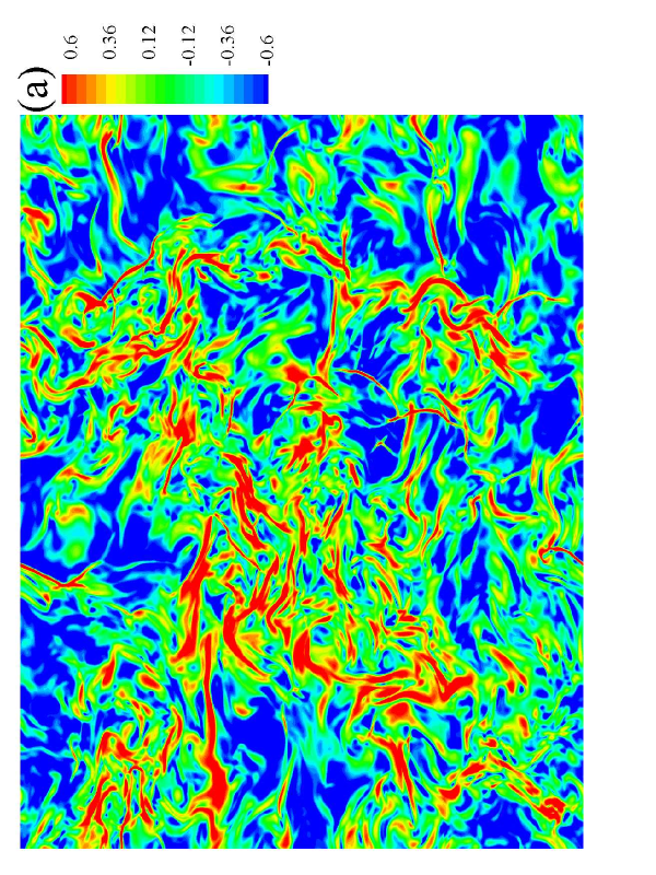
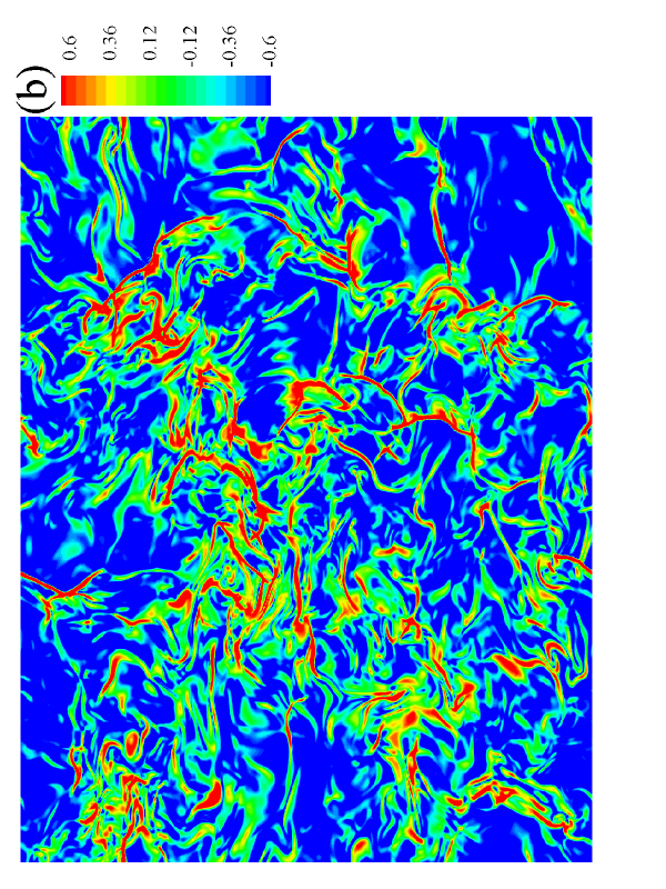
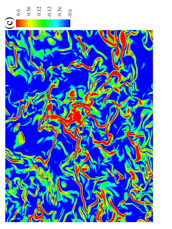
In a stationary state, the kinetic energy and scalar dissipation rates oscillate in space. These oscillations are considered to cause field intermittency. It is therefore valuable to study the spatial structures of dissipation rates. Figure 19 depicts the two-dimensional slices (x-y plane) through the dissipation fields simultaneously in the position of . In order to observe the detailed structures at both small and large amplitudes, we plot the logarithms of dissipation rates, where the color scale is determined by the formulas as follows
| (39) |
| (40) |
Here the colored range is . As dissipation increases, the color changes from blue to red. The kinetic energy dissipation rate is shown in Figure 19(a). We find that the small-scale, high-dissipation regions, separated by the large-scale, low-dissipation regions, distribute discretely and randomly. These regions exhibit as sharp ridges. By contrast, the low-dissipation regions are more or less like deep canyons. Figure 19(b) shows the dissipation rate of temperature, it is consisted of the small-scale, cliff-like high-dissipation regions and the large-scale, ramp-like low-dissipation regions. Here the widths of the small-scale structures are even finer, meaning less dissipation. In Figure 19(c), though the large-scale structures are similar to those shown in the former two panels, the small-scale structures are broader in widths, displaying as ribbons and thus indicating more dissipation.
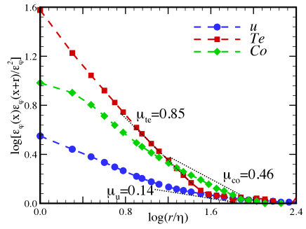
A common used method for quantifying intermittency is to compute intermittency parameter through the auto correlation of dissipation rate, namely
| (41) |
where is the so-called intermittency parameter, and is for , or . The readers can find detailed definition in Wang et al. (1999). In Figure 20 we present the log-log plot of the auto correlations of , and , as functions of the normalized separation distance . There appear three linear regions for the auto correlations, in which , and . The relation of is in agreement with the fact that in our simulation, the intermittency of velocity, concentration and temperature increases sequentially. It should be noted that various methods (i.e. correlation method & variance method) may yield quite different values of intermittency parameter.
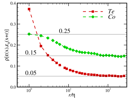
Having analyzed the auto correlation, we shall now report on the correlation between the dissipation rates of kinetic energy and scalars. In Figure 21 we plot the correlation coefficients between and , as functions of the normalized separation distance , which are defined by
| (42) |
It shows that throughout scale ranges, both and have positive correlations. The general behaviors of these correlation coefficients are that they decrease with scale and appear plateaus at the scales larger than , where the level values are and , respectively. Note that the variation of correlation coefficient against scale in this study is opposite to that in incompressible turbulence (Wang et al., 1999), in which the correlation coefficient grows with scale. In the range of , is larger than , namely, the temperature is more closely connected with the velocity. Nevertheless, as scale increases, this connection is weakened and is surpassed by the concentration. Furthermore, at small scales, is saturated at the level value of , whereas there is no saturation observed for .
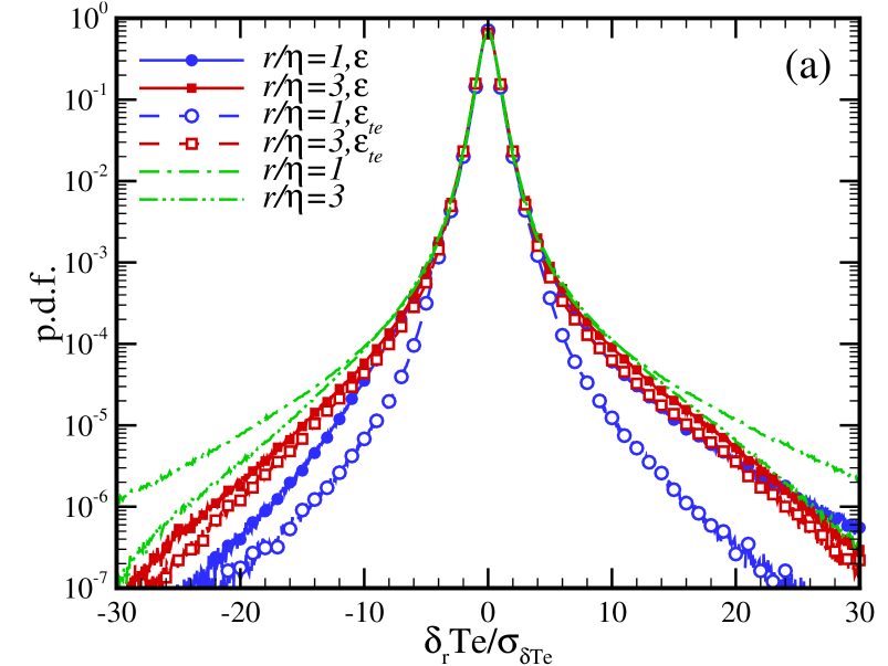
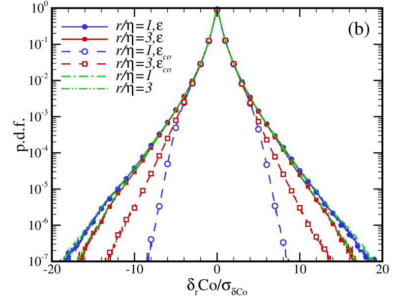
Finally, we turn to discuss the statistical dependence of scalar increment on dissipation rate. In Figure 22 we plot the p.d.f.s of the normalized scalar increments conditioned on dissipation rates at the normalized separation distances of , . For comparison, we also plot the unconditional p.d.f.s at the same separation distances. In the left panel, at each scale, the p.d.f. of temperature increment conditioned on the kinetic energy dissipation rate, , is wider than that conditioned on the temperature dissipation rate, . Moreover, and become narrower as decreases, implying that in the dissipative range, the effects of dissipations make the large fluctuations of temperature happen less frequently at smaller scales. For each scale, the tails of are longest, indicating that the dissipations suppress the intermittency of temperature increment. In the right panel, at each scale, and basically overlap each other, and are wider than . Unlike the case, becomes wider but becomes narrower as falls. Based on the above results, a conclusion is given that in compressible turbulence, the active scalar increment depends both on the kinetic energy and scalar dissipations, while the passive scalar increment mainly relates to the scalar dissipation.
6 Cascades of active and passive scalars
In this section, we employ a ”coarse-graining” approach (Aluie, 2011; Aluie et al., 2012; Aluie, 2013) to study the cascades of active and passive scalars. We begin with the definition of a classically filtered field
| (43) |
where is the kernel, and is a window function. The density-weighted Favre filtered field is then defined by
| (44) |
By the large-scale continuity and temperature equations, it is straightforward to derive the temperature variance budget for large scales as follows
| (45) |
Here is the spatial transport of large-scale temperature variance, is the subgrid-scale (SGS) temperature flux to scales , is the large-scale pressure-dilatation, and are the viscous and temperature dissipations acting on scales , respectively, and is the temperature ”energy” depletion caused by cooling function. The details of these terms are written as
| (46) |
| (47) |
| (48) |
| (49) |
| (50) |
Henceforth, we shall take the liberty of dropping subscript l whenever there is no risk of ambiguity. Similarly, the concentration variance budget for large scales is read as
| (51) |
where is the concentration ”energy” injection from external forcing. The expressions of the spatial transport of large-scale concentration variance, ; the SGS concentration flux to scales , (x); and the molecular dissipation acting on scales , , are
| (52) |
| (53) |
| (54) |

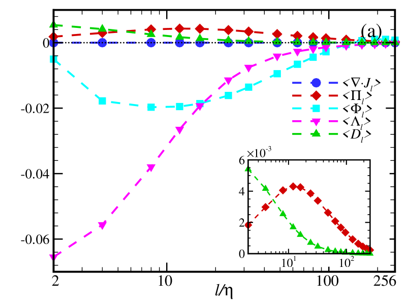
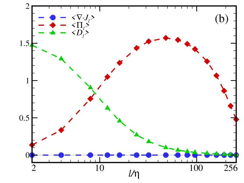
In Figure 23 we plot all the terms in Equations (6.3) and (6.9) except the forcing ones, as functions of the normalized scale . In the statistically homogeneous turbulence, the spatial transport of large-scale temperature variance vanishes, and thus, the value of the corresponding term shown in the left panel is basically zero. Throughout scale ranges, the SGS temperature flux and temperature dissipation are positive, causing the temperature variance to decay. Contrarily, as scale increases, the magnitude of viscous dissipation declines quickly and approaches zero at the scales of , while that of pressure-dilatation first increases and undergoes a flat region in the range of , then decreases and reaches zero at large scales. Note that both the viscous dissipation and pressure-dilatation lead to the amplification of temperature variance. The above observation shows that the action of viscous dissipation is restricted at small scales, while the pressure-dilatation mainly takes place at the moderately large scales satisfying . In the inset we enlarge the temperature dissipation and SGS temperature flux. It is found that the former limits itself at small scales and falls quickly as scale increases. By contrast, for the latter, there appears a plateau spanning the range of , which demonstrates the existence of an inertial range for the temperature cascade. Throughout scale ranges in the right panel, the spatial transport of large-scale concentration variance vanishes as well. The molecular dissipation depletes concentration variance and occurs mainly at small scales. As scale increases, the SGS concentration flux first increases and undergoes a flat region of , then decreases at large scales. It implies that there is only direct cascade in the concentration transport, which is different from that in 1D compressible turbulence (Ni & Chen, 2012).
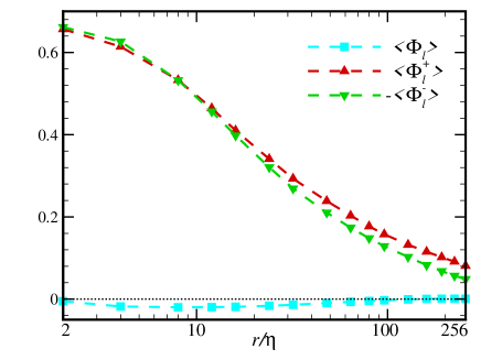
The pressure-dilatation does not contain any modes at scales , and thus, vanishes in the absence of SGS fluctuations. It only contributes to the conversion between the large-scale kinetic and internal energy, namely, if , the energy is transported from kinetic to internal energy; if , the process reverses (Aluie, 2011). The picture of the negligible at small scales does not contradict to the fact of the rarefaction and compression motions appearing at all scales, which are the main property of compressible turbulence. Our result reveals that the high pressure-dilatation generated in the vicinity of small-scale shocklets will vanish after taking global averages, because of the cancelations between rarefaction and compression regions (Aluie et al., 2012). In Figure 24 we plot the pressure-dilatation and its positive and negative components, as functions of the normalized scale . Obviously, both and are high at small scales, however, when adding together, they basically cancel each other and make the outcome be small.
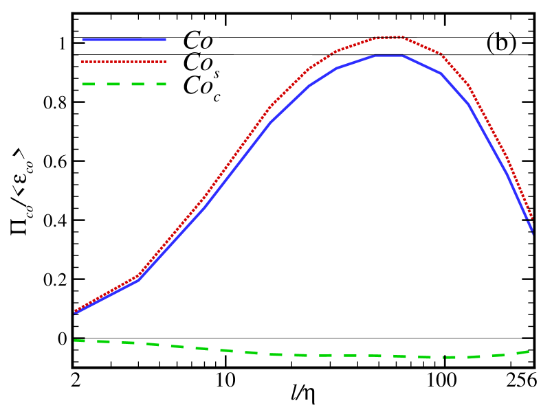
In Figure 25 we plot the normalized SGS scalar fluxes and their components, as functions of the normalized scale . In the left panel, there is a flat region in the range of , indicating the conservation of temperature cascade. The compressive component is significantly larger than the solenoidal component. This reveals that the cascade of temperature is mainly determined by the motions of rarefaction and compression. By contrast, in the right panel, the plateau of the SGS concentration flux appears in the range of , and the level value is close to unity. The magnitude of the solenoidal component is much higher than that of the compressive component. This means that the cascade of concentration is governed by the stretching and shearing of vortices. Furthermore, it is found that the compressibility of turbulence leads the compressive SGS concentration flux to be negative, and thus, trasfer from small to large scales. In a word, our results indicate that the cascades of the active and passive scalars are separately dominated by the compressive and solenoidal components of velocity.
.
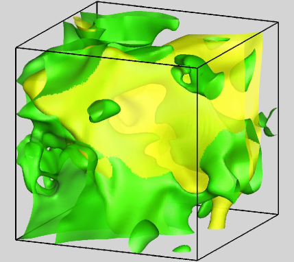
In Figure 26, the 3D isosurfaces of the compressive component of the SGS scalar fluxes, and , are displayed in a same subdomain, where the filter width is . It shows that the sheetlike surfaces of are converged together, similar to the surfaces of dilatation shown in Figure 16. This confirms the dominance of the rarefaction and compression motions in the temperature cascade. By contrast, the surfaces of are broken down into a large number of sheetlike fragments.
.
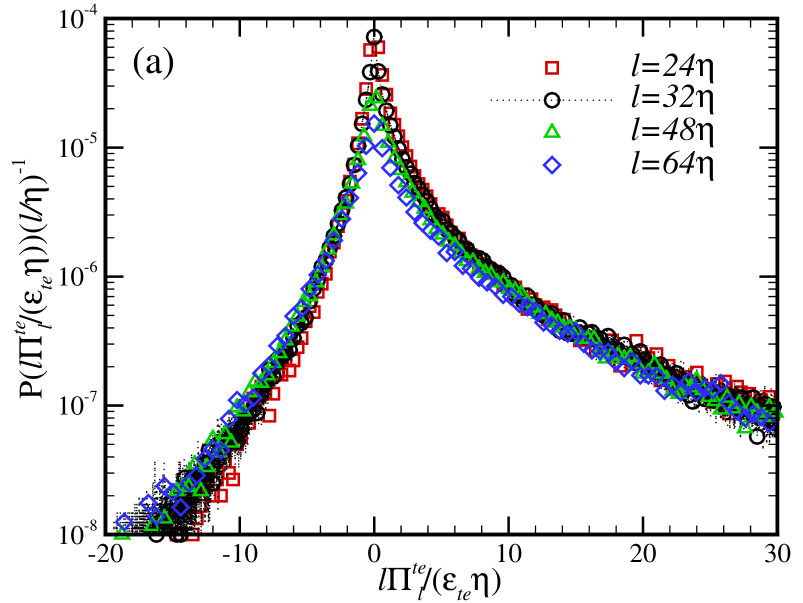
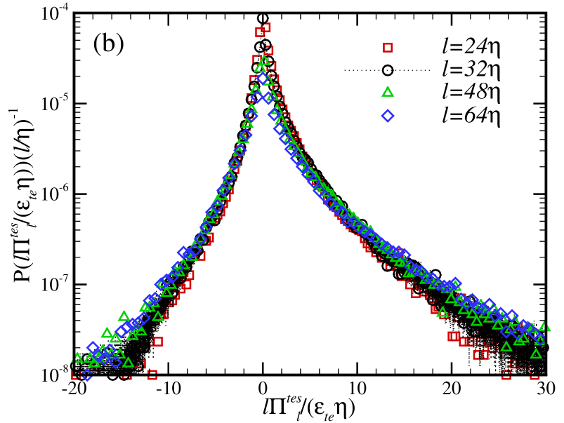
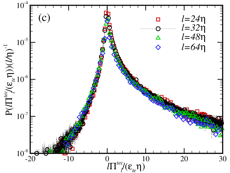
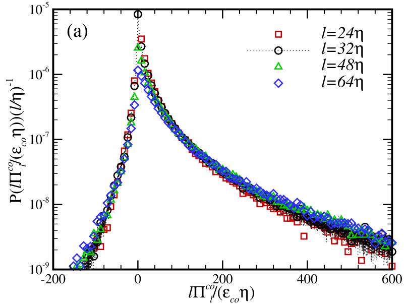
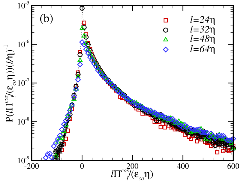
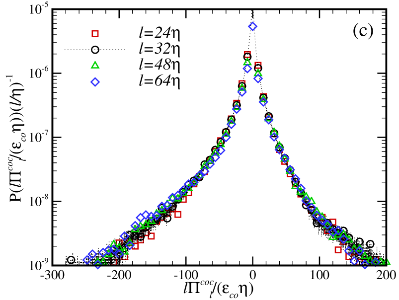
The rescaled p.d.f.s of the SGS scalar fluxes and their components at , , and are plotted in Figure 27 (temperature) and Figure 28 (concentration). It shows that all the rescaled p.d.f.s of , and exhibit skewness toward positive side, therefore, the transfer of temperature flux is completely from large to small scales. By contrast, the rescaled p.d.f.s of and are positively skewed, whereas that of is negatively skewed. It indicates that the compressive component of the concentration flux transfers upscale. Here we point out that the p.d.f. tails of the SGS scalar fluxes are mainly contributed from the small-scale shocklets. Furthermore, we observe that in both figures, the rescaled p.d.f.s collapse to the same distribution for all in the inertial range of . By the multifractal theory (Benzi et al., 2008), the scaling exponents of the statistical moments of and as well as their components should saturate at high order numbers, where the values of exponents are equal to unity. This prediction reveals the statistical scale-invariant property of the active and passive scalar fluxes in the inertial range. Finally, the geometrical similarities of the rescaled p.d.f.s between (, ) and (, ), once again confirm the fact that the cascades of the active and passive scalars are respectively dominated by the compressive and solenoidal components of velocity.
7 Summary and conclusions
In this paper, a systematic investigation on the statistics of active and passive scalars in an isotropic compressible turbulent velocity was performed. The simulation was solved numerically using a hybrid method of a seventh-order WENO scheme for shock region and an eighth-order CCFD scheme for smooth region outside shock. The large-scale velocity and passive scalar forcings were added to drive the simulated system, and maintain it in a stationary sate, where the turbulent Mach number was , and the Taylor microscale Reynolds number was . To explore the statistical differences between active and passive scalars, a variety of statistics including spectrum, structure function, probability distribution function, flow structure and cascade were investigated. Moreover, the effects of solenoidal and compressive processes of velocity on the scalar transports were described, of which some affect both active and passive scalars, while the others are shown to associate with only one scalar.
The spectra of kinetic energy and scalars defer to the power law. The Kolmogorov constant was found to be , while the OC constant for passive scalar is , which is consistent with the typical values observed in incompressible turbulence. Compared to passive scalar, the transfer flux spectrum of active scalar shifts towards higher wavenumbers, since the OC scale of temperature is larger than that of concentration. The local scaling exponents computed from the second-order structure function display flat regions for velocity and active scalar. Nevertheless, for passive scalar, it takes first a minimum of and then a maximum of . Our results also confirmed that the velocity and passive scalar satisfy the Kolmogorov’s 4/5 and Yaglom’s 4/3-laws, respectively. However, there is no similar law found for active scalar.
We then discussed the probability distribution function. First, the p.d.f.s of velocity and active scalar fluctuations are very close to Gaussian at small amplitudes and become super-Gaussian at large amplitudes, while that of passive scalar fluctuations arises slight oscillations at small amplitudes and changes into sub-Gaussian at large amplitudes. Second, the p.d.f. of velocity increment is concave and strongly intermittent at small scales. As scale increases, it approaches Gaussian. Further, by applying the Helmholtz decomposition to velocity, we found that at small scales, the p.d.f. for the solenoidal component of velocity is similar to that for velocity increment in incompressible turbulence, while the p.d.f. for the compressive component of velocity can be analogous to that for velocity increment in Burgers turbulence. As for the scalar increments, the p.d.f.s are symmetric and close to Gaussian at large scales. The shape for the p.d.f. of active scalar increment is concave, and that for the p.d.f. of passive scalar increment is convex, the same to that in incompressible turbulence. Third, the major contributions to the p.d.f. tails of flow gradients are caused by small-scale shocklets rather than large-scale shock waves, which make the values of the power-law exponents be for velocity, for active scalar, and for passive scalar. Furthermore, our results showed that the skewness for velocity and passive scalar increments are positive, and approach zero as scale increases. Throughout scale ranges, in magnitude the skewness of passive scalar increment is always smaller than that of velocity increment, indicating a weaker degree of Gaussian departure.
In terms of high-order statistics, the scaling exponent computed from structure function gives the following relations: , , and , where the last one is similar to that observed in incompressible turbulence. In addition, the computation based on the Helmholtz decomposition revealed that is nearly identical to the mixed temperature-velocity scaling exponent shown in previous 1D compressible turbulence simulation.
We further investigated the field structures of scalars. It seemed that the active scalar has the ”ramp-cliff” structures, which is usually regarded as production by stretching and shearing of vortices. By contrast, the passive scalar is dominated by the large-scale rarefaction and compression caused by shock fronts. The visualization of the isosurfaces of dilatation and scalars provides conclusions in two respects: (1) the sheetlike active scalar surfaces are wrinkled, distribute around shock wave and intersect with the dilatation surfaces in certain positions; and (2) the passive scalar surfaces are also sheetlike, and the opposite-sign value basically appears on each side of the shock fronts. The statistics of angles between vorticity and scalar gradients show that the scalar gradients prefer to be perpendicular to the vorticity. Compared to active scalar, the p.d.f. of passive scalar is much steeper, showing that the passive scalar is more frequently tangent to the vorticity.
The analysis of dissipation field structures started from the dissipation spectra of scalars. We found that the maximum dissipation spectrum of passive scalar locates at higher wavenumbers than that of active scalar, given that the effectively smallest scale for passive scalar is about , smaller than the Kolmogorov scale. In the range of , the dissipation spectra approximately follow a scaling, which can be derived from the Komlogorov theory. In order to understand the detailed structures at both small and large amplitudes, we computed the logarithms of the scalar dissipation rates: and . It showed that is composed of the small-scale cliff-like structures of high dissipation and the large-scale ramp-like structures of low dissipation. By contrast, the small-scale structures in are broader in widths, and display as ribbons. The exponent parameter computed from the auto correlation of dissipation rate is a common used method for quantifying intermittency. Our results gave that and , meaning that the active scalar is much stronger in intermittency. As for the correlation coefficients between the dissipation rates of kinetic energy and scalars, it showed that and decrease with scale and emerges plateaus at scales larger than . At small scales, saturates at the level value of . The analysis was completed by the statistical dependence of scalar increment on dissipation rate. We found that the active scalar increment suffers influence from both the kinetic energy and active scalar dissipations, while the passive scalar increment mainly connects with its own dissipation.
By employing a ”coarse-graining” approach, the scalar variance budgets for large scales were obtained. First, we observed that throughout scale ranges, the active scalar variance is increased by the large-scale pressure-dilatation and small-scale viscous dissipation, but is decreased by the SGS flux and temperature dissipation. The decomposition on pressure-dilatation showed that it has high values in the vicinity of small-scale shocklets. However, because of the cancelations between rarefaction and compression regions, the contribution vanishes after space average. As for passive scalar variance, it is depleted by the molecular dissipation at small scales, and is transported by the SGS flux from large to small scales. Second, the SGS active scalar flux, dominated by its compressive component, appears a plateau in the range of , implying the conservation of active scalar cascade. In spite of the compressive component is negative, the much larger positive solenoidal component leads the SGS passive scalar flux to transfer downscale as well, and defines the conservative cascade of passive scalar in the range of . As a result, in our simulation, the transport of passive scalar is mainly determined by the solenoidal component of velocity, which is similar to that in incompressible turbulent flows. Furthermore, the visualization for the isosurfaces of compressive-component SGS scalar flux at the filter width confirms the dominance of the motions of rarefaction and compression in the active scalar cascade. Third, it was found that in the inertial range, the rescaled scalar flux p.d.f.s collapse to the same distribution. According to the mutifractal theory, we predicted that the scaling exponents for the moments of and should saturate at high order numbers. This indicates that there are scale-invariant features for the statistics of active and passive scalars. In addition, the geometrical similarities of the rescaled p.d.f.s once again prove the aforementioned conclusion that the cascades of active and passive scalars are separately dominated by the compressive and solenoidal components of velocity.
The current investigation reveals a variety of unique small-scale features of active and passive scalars in compressible turbulence, relative to the statistical properties of passive scalar in incompressible turbulence. Here we limit our study to the large-scale solenoidal forcing, a complementary numerical simulation in which both the solenoidal and compressive components of velocity are stirred will be performed (Ni & Chen, 2015). Our future work will also address the effects of basic parameters such as the Mach and Schmidt numbers on the scalar transport in compressible turbulence (Ni, 2015a, b).
8 Acknowledgement
We thank Dr. J. Wang for many useful discussions. This work was supported by the National Natural Science Foundation of China (Grant 11221061) and the National Basic Research Program of China (973) (Grant 2009CB724101). Q. N. acknowledges partial support by China Postdoctoral Science Foundation Grant 2014M550557. Simulations were done on a cluster computer in the Center for Computational Science and Engineering at Peking University and on the TH-1A supercomputer in Tianjin, National Supercomputer Center of China.
References
- Aluie (2011) Aluie, H. 2011 Compressible turbulence: the cascade and its locality. Phys. Rev. Lett. 106, 174502.
- Aluie et al. (2012) Aluie, H., Li, S. & Li, H. 2012 Conservative cascade of kinetic energy in compressible turbulence. Astrophy. J. 751, L29.
- Aluie (2013) Aluie, H. 2013 Scale decomposition in compressible turbulence. Physica D 247, 54–65.
- Andreopoulos et al. (2000) Andreopoulos, Y., Agui, J. H. & Briassulis, G. 2000 Shock wave-turbulence interactions. Annu. Rev. Fluid Mech. 32, 309–345.
- Antonia & Orlandi (2003) Antonia, R. A. & Orlandi, P. 2003 On the Batchelor constant in decaying isotropic turbulence. Phys. Fluids 15, 2084–2086.
- Balkovsky & Lebedev (1998) Balkovsky, E. & Lebedev, V. 1998 Instanton for the Kraichnan passive scalar problem. Phys. Rev. E 58, 5776–5795.
- Balsara & Shu (2000) Balsara, D. S. & Shu, C. W. 2000 Monotonicity preserving weighted essentially non-oscillatory schemes with increasingly high order of accuracy. J. Comp. Phys. 160, 405–452.
- Batchelor (1959) Batchelor, G. K. 1959 Small-scale variation of convected quantities like temperature in turbulent flows. J. Fluid. Mech. 5, 113–120.
- Bec et al. (2000) Bec, J., Frisch, U. & Khanin, K. 2000 Kicked Burgers turbulence. J. Fluid Mech. 416, 239–267.
- Benzi et al. (2008) Benzi, R., Biferale, L., Fisher, R. T., Kadanoff, L. P., Lamb, D. Q. & Toschi, F. 2008 Intermittency and university in fully developed inviscid and weakly compressible turbulent flows. Phy. Rev. Lett. 100, 234503.
- Cao & Chen (1997) Cao, N. & Chen, S. 1997 An intermittency model for passive scalar. Phys. Fluids 9, 1203.
- Cartledge et al. (2006) Cartledge, S. I. B., Lauroesch, J. T., Meyer, D. M. & Sofia, U. J. 2006. The homogeneity of interstellar elemental abundances in the galactic disk. Astrophys. J. 641, 327.
- Celani et al. (1999) Celani, A., Lanotte, A. & Mazzino, A. 1999 Passive sclar intermittency in compresible flow. Phys. Rev. E 60, R1138.
- Celani et al. (2002a) Celani, A., Matsumoto, T., Mazzino, A. & Vergassola, M. 2002 Scaling and universality in turbulent convection. Phys. Rev. Lett. 88, 054503.
- Celani et al. (2002b) Celani, A., Cencini, M., Mazzino, A. & Vergassola, M. 2002 Active versus passive scalar turbulence. Phys. Rev. Lett. 89, 234502.
- Celani et al. (2004) Celani, A., Cencini, M., Mazzino, A. & Vergassola, M. 2004 Active and passive fields face to face. New J. Phys. 6, 72.
- Chen & Kraichnan (1998) Chen, S. & Kraichnan, R. H. 1998 Simulations of a randomly advected passive scalar field. Phys. Fluids 10, 2867–2884.
- Chertkov et al. (1997) Chertkov, M., Kolokolov, I. & Vergassola, M. 1997 Inverse cascade and intermittency of passive scalar in one-dimensional smooth flow. Phys. Rev. E 56, 5483–5499.
- Chertkov et al. (1998) Chertkov, M., Kolokolov, I. & Vergassola, M. 1998 Inverse versus direct cascades in turbulent advection. Phys. Rev. Lett. 80, 512–515.
- Ching et al. (2003) Ching, E. S. C., Cohen, Y., Gilbert, T. & Procaccia, I. 2003 Active and passive fields in turbulent transport: the role of statistically preserved structures. Phys. Rev. E 67, 016304.
- Corrsin (1951) Corrsin, S. 1951 On the spectrum of isotropic temperature fluctuations in an isotropic turbulence. J. Appl. Phys. 22, 469–473.
- Donzis et al. (2010) Donzis, D. A., Sreenivasan, K. R. & Yeung, P. K. 2010 The Batchelor spectrum for mixing of passive scalars in isotropic turbulence. Flow Turbulence Combust. 85, 549.
- E & Eijnden (1999) E, W. & Eijnden, E. V. 1999 Asymptotic theory for the probability density function in Burgers turbulence. Phys. Rev. Lett. 83, 2572–2575.
- E & Eijnden (2000) E, W. & Eijnden, E. V. 2000 Statistical theory for the stochastic Burgers equation in the inviscid limit. Comm. Pure Appl. Math. 53, 877.
- Erlebacher & Sarkar (1993) Erlebacher, G. & Sarkar, S. 1993 Statistical analysis of the rate of strain tensor in compressible homogeneous turbulence. Phys. Fluids A 5, 3240–3254.
- Gawedzki & Vergassola (2000) Gawedzki, K. & Vergassola, M. 2000 Phase transition in the passive scalar advection. Physica D 138, 63–90.
- Ishihara et al. (2007) Ishihara, T., Kaneda, Y., Yokokawa, M., Itakura, K. & Uno, A. 2007 Small-scale statistics in high-resolution direct numerical simulation of turbulence: Reynolds number dependence of one-point velocity gradient statistics. J. Fluid Mech. 592, 335–366.
- Ishihara et al. (2009) Ishihara, T., Gotoh, T. & Kaneda, Y. 2009 Study of high-Reynolds number isotropic turbulence by direct numerical simulation. Annu. Rev. Fluid Mech. 41, 165–180.
- Kholmyansky et al. (2001) Kholmyansky, M., Tsinober, A. & Yorish, S. 2001 Velocity derivatives in the atmospheric surface layer at . Phys. Fluids 13, 311–314.
- Kolmogorov (1941) Kolmogorov, A. N. 1941 The local structure of turbulence in incompressible viscous fluid for very large Reynolds numbers. Dokl. Akad. Nauk SSSR 30, 9.
- Kraichnan (1994) Kraichnan, R. H. 1994 Anomalous scaling of a randomly advected passive scalar. Phys. Rev. Lett. 72, 1016.
- Lele (1992) Lele, S. K. 1992 Compact finite difference schemes with spectral-like resolution. J. Comp. Phys. 103, 16–42.
- Lu & Turco (1994) Lu, R. & Turco, R. P. 1994 Air pollutant transport in a coastal environment. Part I: two-dimensional simulations of sea-breeze and mountain effects. J. Atmos. Sci. 51, 2285–2308.
- Lu & Turco (1995) Lu, R. & Turco, R. P. 1995 Air pollutant transport in a coastal environment-II. three-dimensional simulations over Los Angeles basin. Atmos. Environ. 29, 1499–1518.
- Meyer et al. (1998) Meyer, D. M., Jura, M. & Cardelli, J. A. 1998 The definitive abundance of interstellar Oxygen. Astrophys. J. 493, 222.
- Monin (1975) Monin, A. S. 1975 Statistical fluid mechanics. Massachusetts Institute of Technology vol. II.
- Mydlarski & Warhaft (1998) Mydlarski, L. & Warhaft, Z. 1998 Passive scalar statistics in high-Peclet-number grid turbulence. J. Fluid Mech. 358, 135–175.
- Ni & Chen (2012) Ni, Q. & Chen, S. 2012 Statistics of active and passive scalars in one-dimensional compressible turbulence. Phys. Rev. E 86, 066307.
- Ni et al. (2013) Ni, Q., Shi Y. & Chen, S. 2013 Statistics of one-dimensional compressible turbulence with random large-scale force. Phys. Fluids 25, 075106.
- Ni & Chen (2015) Ni, Q. & Chen, S. 2015 Effects of shock structure on temperature field in compressible turbulence. J. Fluid Mech. to be submitted.
- Ni (2015a) Ni, Q. 2015 Compressible turbulent mixing: Effects of Mach number and forcing scheme. Phys. Rev. E to be submitted.
- Ni (2015b) Ni, Q. 2015 Compressible turbulent mixing: Effects of Schmidt number. Phys. Rev. E accepted.
- Obukhov (1949) Obukhov, A. M. 1949 On the problem of geostrophic wind. Izv. Geogr. Geophys. 13, 281–306.
- Pan & Scannapieco (2010) Pan, L. & Scannapieco, E. 2010 Mixing supersonic turbulence. Astrophy. J. 721, 1765–1782.
- Pan & Scannapieco (2011) Pan, L. & Scannapieco, E. 2011 Passive scalar structures in supersonic turbulence. Phys. Rev. E 83, 045302(R).
- Pirozzoli & Grasso (2004) Pirozzoli, S. & Grasso, F. 2004 Direct numerical simulations of isotropic compressible turbulence: Influence of compressibility on dynamics and structures. Phys. Fluids 16, 4386–4407.
- Pope (1991) Pope, S. B. 1991 Computations of turbulent combustion: progress and challenges. Symposium on Combustion 23, 591–612.
- Pope (2000) Pope, S. B. 2000 Turbulent flows. Cambridge University Press.
- Porter et al. (2002) Porter, D., Pouquet, A. & Woodward, P. 2002 Measures of intermittency in driven supersonic flows. Phys. Rev. E 66, 026301.
- Samtaney et al. (2001) Samtaney, R., Pullin, D. I. & Kosovic, B. 2001 Direct numerical simulation of decaying compressible turbulence and shocklet statistics. Phys. Fluids 13, 1415–1430.
- She & Leveque (1994) She, Z. S. & Leveque, E. 1994 Universal scaling laws in fully developed turbulence. Phys. Rev. Lett. 72, 336–339.
- Shraiman & Siggia (1994) Shraiman, B. I. & Siggia, E. D. 1994 Lagrangian path integrals and fluctuations in random flow. Phys. Rev. E 49, 2912–2927.
- Shraiman & Siggia (2000) Shraiman, B. I. & Siggia, E. D. 2000 Scalar turbulence. Nature 405, 639.
- Sreenivasan (1996) Sreenivasan, K. R. 1996 The passive scalar spectrum and the Obukhov-Corrsin constant. Phys. Fluids 8, 189–196.
- Sutherland (1992) Sutherland, W. 1992 The viscosity of gases and molecular force. Philos. Mag. Suppl. 5, 507–531.
- Wang et al. (1996) Wang, L.-P., Chen, S., Brasseur, J. G. & Wyngaard, J. C. 1996 Examination of hypotheses in the Kolmogorov refined turbulence theory through high-resolution simulations. Part 1. Velocity field. J. Fluid Mech. 309, 113–156.
- Wang et al. (1999) Wang, L.-P., Chen, S. & Wyngaard, J. C. 1999 Examination of hypotheses in the Kolmogorov refined turbulence theory through high-resolution simulations. Part 2. Passive scalar field. J. Fluid Mech. 400, 163–197.
- Wang et al. (2010) Wang, J., Wang, L.-P., Xiao, Z., Shi, Y. & Chen, S. 2010 A hybrid approach for direct numerical simulation of isotropic compressible turbulence. J. Comp. Phys. 229, 5257–5279.
- Wang et al. (2012a) Wang, J., Shi, Y., Wang, L.-P., Xiao, Z., He, X. & Chen, S. 2012 Scaling and statistics in three-dimensional compressible turbulence. Phys. Rev. Lett. 108, 214505.
- Wang et al. (2012b) Wang, J., Shi, Y., Wang, L.-P., Xiao, Z., He, X. & Chen, S. 2012 Effect of compressibility on the small-scale structures in isotropic turbulence. J. Fluid Mech. 713, 588–631.
- Warhaft (2000) Warhaft, Z. 2000 Passive scalars in turbulent flows. Annu. Rev. Fluid Mech. 32, 203–240.
- Watanabe & Gotoh (2004) Watanabe, T. & Gotoh, T. 2004 Statistics of a passive scalar in homogeneous turbulence. New J. Phys. 6, 40.
- Watanabe & Gotoh (2007) Watanabe, T. & Gotoh, T. 2007 Inertial-range intermittency and accuracy of direct numerical simulation for turbulence and passive scalar turbulence. J. Fluid Mech. 590, 117.
- Yaglom (1949) Yaglom, A. M. 1949 On the local structure of the temperature field in a turbulent flow. Dokl. Akad. Nauk SSSR 69, 6.
- Yeung et al. (2002) Yeung,P. K., Xu, S. Y. & Sreenivasan, K. R. 2002 Schmidt number effects on turbulent transport with uniform mean scalar gradient. Phys. Fluids 14, 4178.
- Yeung et al. (2004) Yeung,P. K., Xu. S, Donzis, D. A. & Sreenivasan, K. R. 2004 Simulations of three-dimensional turbulent mixing for Schmidt number of the order 1000. Flow Turbulence Combuts. 72, 333.
- Yeung et al. (2005) Yeung,P. K., Donzis, D. A. & Sreenivasan, K. R. 2005 High-Reynolds-number simulation of turbulent mixing. Phys. Fluids 17, 081703.
- Yeung & Sreenivasan (2012) Yeung,P. K. & Sreenivasan, K. R. 2012 Spectrum of passive scalars of high molecular diffusivity in turbulent mixing. J. Fluid Mech. 716, R14.
- Yeung & Sreenivasan (2014) Yeung,P. K. & Sreenivasan, K. R. 2014 Direct numerical simulation of turbulent mixing at very low Schmidt number with a uniform mean gradient. Phys. Fluids 26, 015107.
- Zhou & Xia (2002) Zhou, S. Q. & Xia, K. Q. 2002 Plume statistics in thermal turbulence: mixing of an active scalar. Phys. Rev. Lett. 89, 184502.