Socio-Spatial Group Queries for Impromptu Activity Planning

Abstract

The development and integration of social networking services and smartphones have made it easy for individuals to organize impromptu social activities anywhere and anytime. Main challenges arising in organizing impromptu activities are mostly due to the requirements of making timely invitations in accordance with the potential activity locations, corresponding to the locations of and the relationships among the candidate attendees. Various combinations of candidate attendees and activity locations create a large solution space. Thus, in this paper, we propose Multiple Rally-Point Social Spatial Group Query (MRGQ), to select an appropriate activity location for a group of nearby attendees with tight social relationships. We first consider a special case of MRGQ, namely the Socio-Spatial Group Query (SSGQ), to determine a set of socially acquainted attendees while minimizing the total spatial distance to a specific activity location. We prove that SSGQ is NP-hard and formulate an Integer Linear Programming optimization model for SSGQ. We then develop an efficient algorithm, called SSGS, which employs effective pruning techniques to reduce the running time to determine the optimal solution. Moreover, we propose a heuristic algorithm for SSGQ to efficiently produce good solutions. We next consider the more general MRGQ. Although MRGQ is NP-hard, the number of attendees in practice is usually small enough such that an optimal solution can be found efficiently. Therefore, we first propose an Integer Linear Programming optimization model for MRGQ. We then design an efficient algorithm, called MAGS, which employs effective search space exploration and pruning strategies to reduce the running time for finding the optimal solution. We also propose to further optimize efficiency by indexing the potential activity locations. A user study demonstrates the strength of using SSGS and MAGS over manual coordination in terms of both solution quality and efficiency. Experimental results on real datasets show that our algorithms can process SSGQ and MRGQ efficiently and significantly outperform other baseline algorithms, including one based on the commercial parallel optimizer IBM CPLEX.

1 Introduction

The successful development and integration of social networking services and smartphones have driven the recent emergence of location-based social networking (LBSN) services. Such services, including applications on Foursquare, Meetup, Facebook, and Google+, allow users to connect with friends, comment on events and places (e.g., restaurants, theaters, stores, etc.), and share their happenings and current locations. This availability of users’ locations and their social information allows mobile users to instantly organize impromptu social activities anywhere anytime.

As an LBSN application, an impromptu activity planning service needs to account for both spatial and social factors. In other words, both the locations and friends considered need to be suitable for the activity, i.e., the location should be close to the participants so that they arrive in a timely manner, and the invited friends should already be acquainted with each other to ensure comity. Thus, a major challenge for impromptu activity planning lies in factoring in the distances from invitees’ current locations to the activity locations, along with their shared social connectivity. Note that close friends may not be located near a specific activity location, while friends near a potential activity location may not enjoy tight social relationships. Moreover, when the number of candidate attendees increases, or when the number of activity locations grows, selecting the most suitable attendees and activity location becomes tedious and time-consuming. Therefore, impromptu activity planning would benefit significantly from efficient query processing algorithms that automatically recommend both attendees and an activity location.

Figure 1: Finding friends for impromptu social activity.

Motivating Example. The interplay of social relationships among activity attendees and the activity locations creates significant challenges for the organization of impromptu social activities. Figure 1 shows a database of 8 candidate attendees $\{v_{1},..,v_{8}\}$ with three potential activity locations $Q=\{q_{1},q_{2},q_{3}\}$. The social relationships among the candidate attendees are captured as a social graph (shown as the social layer in the figure), while the locations of the candidate attendees are shown as the spatial layer. Given a desired group size, $4$, and a social constraint where each attendee can only be unfamiliar with at most $1$ other attendee, an approach to select a group and the corresponding activity location with minimized total spatial distance is to issue a 4-nearest neighbor (4NN) query on each activity location. In the result, we obtain $F_{1}=\{v_{2},v_{3},v_{4},v_{5}\}$ with the activity location $q_{1}$. However, in this case, $F_{1}$ does not satisfy the required social constraint because both $v_{2}$ and $v_{3}$ are unacquainted with more than $1$ other group member. Instead, if we focus on social tightness, we obtain group $F_{2}=\{v_{1},v_{6},v_{7},v_{8}\}$ with activity location $q_{2}$, where each attendee is familiar with all the other members. However, this group incurs a large spatial distance and thus is not suitable for an impromptu activity. In contrast, $F_{3}=\{v_{1},v_{2},v_{5},v_{6}\}$ with activity location $q_{3}$ is probably the most suitable solution because each attendee in $F_{3}$ is unacquainted with no more than $1$ other group member while incurring a small total spatial distance to $q_{3}$.

In this paper, we propose a new query, namely Multiple Rally-Point Social Spatial Group Query (MRGQ), to determine a suitable activity location and a socially acquainted group which minimizes the total spatial distance to the activity location. MRGQ seeks a set of most-suitable attendees with a corresponding activity location by considering both social and spatial factors of impromptu activity planning. MRGQ is beneficial for real social network applications (e.g., Facebook) and can integrate with group buying websites (e.g., Groupon) to provide social-aware location-based advertisements. We will discuss these issues in Section 2.2. Here, we assume that the service provider has access to the users’ underlying social relationships along with their current locations. Let $G=(V,E)$ be a social graph, where each vertex $v\in V$ is associated with a location $l_{v}$, and two mutually acquainted vertices $u$ and $v$ are connected by an edge $e_{u,v}$. Given a set of potential activity locations $Q=\{q_{1},..,q_{n}\}$, the planned number of activity attendees $p$, the number of unacquainted people each attendee may have $k$, and the maximum spatial distance $t$ (i.e., spatial radius) from the chosen activity location to each of the selected attendees, MRGQ aims to find a set of $p$ attendees from the social graph and an activity location $q^{*}$ from the potential activity location list, such that the total distance from each attendee to the activity location $q^{*}$ is minimal, and the distance from each attendee to the activity location $q^{*}$ is bounded by $t$. Notice that MRGQ includes a social constraint (i.e., $k$) to ensure the familiarity between each attendee, i.e., each attendee can be unfamiliar with at most $k$ other people in the selected group. By setting $k$, the coordinator can freely adjust the social atmosphere of the activity to accommodate different types of social activities. Formally, MRGQ is formulated as follows.

Problem: Multiple Rally-Point Social Spatial Group Query (MRGQ).

Given: A social graph $G=(V,E)$, location $l_{v}$ for each $v\in V$, the number of attendees $p$, the set of potential activity locations $Q$, the familiarity constraint $k$, and the spatial radius $t$.

Objective: $MRGQ(p,Q,k,t)$ finds $\langle F,q^{*}\rangle$ where $F\subseteq V$, $q^{*}\in Q$, such that $|F|=p$, $\sum_{v\in F}d_{v,q^{*}}$ is minimal, $d_{v,q^{*}}\leq t$, and $unfamiliar(v,F)$ $\leq k$, $\forall v\in F$.

A straightforward approach for processing MRGQ is to enumerate all possible groups of $p$ attendees for each activity location and eliminate those not satisfying the constraints on social familiarity and spatial radius. Then, this approach returns the pair of group and activity location which incur the minimum total spatial distance. This straightforward approach needs to enumerate $|Q|\cdot C^{|V|}_{p}$ candidate pairs of groups and locations, entailing an enormous search space. Indeed, as we show in the next section, MRGQ is NP-hard. However, as the size of $p$ is relatively small in most practical impromptu activity scenarios, the problem can be solved efficiently. By carefully exploring the social and spatial constraints in MRGQ, we develop several processing strategies to obtain the optimal solution efficiently. We systematically examine the search space to avoid examining all combinations of candidate attendees and the activity locations. We incrementally select attendees with the corresponding activity location by giving priority to those attendees (i) who are close to an activity location, and (ii) who are close friends. Obtaining a group which satisfies both (i) and (ii) is non-trivial because an algorithm that addresses (i) should simultaneously choose suitable attendees and the nearest activity location. However, while achieving (i) may quickly obtain a group with small total spatial distance, it does not always result in a feasible group that satisfies the familiarity constraint. Alternatively, we can address (ii) by prioritizing the search for a group of attendees who know each other well. However, the group may not have the minimum spatial distance to the closest activity location. In summary, efficiently processing MRGQ requires carefully designed algorithms to select the attendees along with their nearby activity location while simultaneously satisfying the familiarity constraint.

To efficiently process MRGQ, we propose to index the attendees’ locations and the activity locations. In addition, we design effective strategies for traversing the search space, including Socio-Spatial Ordering and All-Pair Distance Ordering, as well as a number of search space pruning rules, including Inner-Triangle Distance Pruning, Outer-Triangle Distance Pruning, Activity Location Distance Pruning, and Familiarity Pruning, to reduce the processing time. During the selection of the attendees and the activity location, we address both the spatial distance among the candidate locations, and from attendees to activity locations. Meanwhile, the social connectivity of the attendees is also carefully explored. As such, we effectively prune redundant search space to find the optimal solution efficiently.

The contributions of this paper are summarized as follows.

We identify the organization of impromptu social activities as a new social networking application and formulate a novel query, MRGQ, to obtain the optimal set of invitees and a suitable activity location. MRGQ is unique because it specifies the familiarity constraint among the invitees. We prove that the problem is NP-hard and inapproximable within any factor.

We consider a special case of MRGQ, namely SSGQ, for considering only a single activity location. We prove that SSGQ is NP-hard and propose SSGS with various strategies for finding the optimal solution efficiently. In addition, we propose a heuristic algorithm for SSGQ, namely SSGMerge, which effectively exploits the structures of intermediate solutions, to obtain good solutions in polynomial time. We also propose an Integer Linear Programming (ILP) optimization model for SSGQ and demonstrate that SSGS outperforms ILP.

To efficiently process MRGQ, we propose to index the locations of candidate attendees and the activity locations and propose an efficient algorithm, namely MAGS, which enables various search space traversing and pruning strategies to find the optimal solution efficiently. We also propose an Integer Linear Programming (ILP) optimization model for MRGQ and demonstrate that MAGS outperforms ILP, even if it runs on a commercial integer programming optimizer with parallel computation.

We conduct a user study with 206 people. The results demonstrate that our proposed algorithms significantly outperform manual coordination in terms of both solution quality and efficiency for both SSGQ and MRGQ. We also implement SSGQ in Facebook.

We evaluate the performance of the proposed algorithms by conducting extensive experiments on real datasets. Experimental results manifest that SSGS and SSGMerge require much less time than the ILP optimization model with the commercial parallel optimizer IBM CPLEX [1]. Likewise, for MRGQ, MAGS outperforms the baseline algorithms in terms of both solution quality and efficiency, and is much more efficient than the ILP optimization model.

The rest of this paper is summarized as follows. Section 2 analyzes MRGQ and proves that it is NP-hard. Section 3 introduces the related works. Section 4 studies a special case of MRGQ, namely SSGQ and details the proposed algorithms. Section 5 details the proposed algorithm to efficiently process MRGQ. Section 7 shows the results of our user study and experiments. Finally, Section 8 concludes this paper.

2 Problem Analysis and Applications

An MRGQ includes four parameters, i.e., $p$, $Q$, $k$ and $t$, which respectively determine the size of the answer group, activity locations, familiarity constraint and spatial radius of the query, and all of which have a significant impact on processing strategies. First, as the size of group, $p$, increases, the solution space (which consists of all candidate groups) grows rapidly. While we prove that processing MRGQ is an NP-hard problem and thus very challenging, it can still be processed efficiently since the size of $p$ is usually small in most practical cases. Second, candidate attendees located close to a candidate activity location $q_{i}$ could be prioritized for processing, as the search criteria aim to minimize the total spatial distance from the selected attendees to $q_{i}$. As the size of $Q$ increases, the search space also grows. Third, $k$ dictates the tightness of social relationships among members in the invited group. A smaller $k$ in MRGQ indicates that candidate attendees with tighter social relationships should be given priority. Finally, $t$ reflects the need to avoid selecting candidates that are unacceptably far away from the selected activity location. These spatial and familiarity constraints can be employed for pruning of unqualified candidate groups. In the following, we first analyze the hardness of MRGQ and then discuss concrete application scenarios for MRGQ.

2.1 Problem Analysis

We prove that MRGQ is NP-hard and inapproximable within any factor, i.e., no approximation algorithm exists for MRGQ.

Theorem 1

MRGQ is NP-hard and is inapproximable within any factor unless $P=NP$.

Proof 1

We prove that MRGQ is NP-hard with the reduction from $p$-clique. Decision problem $p$-clique, given a graph $G_{c}$, determines whether the graph contains a clique, i.e., a complete graph of $p$ vertices and with an edge connecting every two vertices. In MRGQ, let $G=G_{c}$, $k=0$, $t=\infty$, $Q=\{q\}$ and $d_{v,q}=1$ for every vertex $v$ $\in V$. We first prove the necessary condition. If $G_{c}$ contains a $p$-clique, there must exist a group with the same vertices in the $p$-clique such that every person has social relationship with all the other attendees in the group, and the total spatial distance is $p$. We then prove the sufficient condition. If $G$ in MRGQ has a group of size $p$ and $k=0$, $G_{c}$ in problem $p$-clique must contain a solution of size $p$, too. Therefore, MRGQ is NP-hard.

We prove the inapproximability of MRGQ with a gap-introducing reduction from the $p$-clique problem. Given a graph $G_{c}$, the decision problem $p$-clique determines whether the graph contains a clique of size $p$, i.e., a complete graph of $p$ vertices with an edge connecting every two vertices. For any instance of the $p$-clique problem in graph $G_{c}$, we construct an instance of MRGQ as follows. The input graph of MRGQ, $G$, is constructed by adding a complete graph $K_{p}$ with $p$ vertices to $G_{c}$, i.e., $G=G_{c}\cup K_{p}$, where each vertex $v\in K_{p}$ connects to every vertex $u\in G_{c}$. We set $Q=\{q\}$, where $q$ is any spatial object, and the spatial distance from each vertex $u\in G_{c}$ to $q$ is set to $1$, i.e., $d_{u,q}=1,\forall u\in G_{c}$. By contrast, the spatial distance from each vertex $v\in K_{p}$ to $q$ is set to an arbitrary value $l$ much larger than $p$, i.e., $d_{v,q}=l,\forall v\in K_{p}$. Moreover, $k=0$ and $t=\infty$ in MRGQ. Now, if there is a $p$-clique in $G_{c}$, there exists a feasible solution of MRGQ, i.e., $F\subseteq G_{c}$ in $G$, with the total spatial distance as $\sum_{v\in F}d_{v,q}=p$ (i.e., $F\cap K_{p}=\varnothing$). If no $p$-clique exists in $G_{c}$, MRGQ has at least one feasible solution, such as $K_{p}$, but it is not possible to extract a feasible solution from $G_{c}$ alone. Therefore, the optimal solution $F$ returned by MRGQ must include at least one vertex in $K_{p}$ with a total spatial distance of $\sum_{v\in F}d_{v,q}\geq(p-1+l)>p$ (i.e., $F\cap K_{p}\neq\varnothing$). MRGQ cannot be approximated within any factor smaller than $(p-1+l)/p$; otherwise, the approximation algorithm could solve the $p$-clique decision problem since it can distinguish the two cases in MRGQ. Since $l$ can be set as an arbitrary value much larger than $p$, MRGQ cannot be approximated within any ratio. The theorem follows.

We also propose an Integer Linear Programming (ILP) optimization model for MRGQ which, via a commercial solver, such as CPLEX [1], can obtain the optimal solution. We first define a number of decision variables in the ILP formulation. Let binary variable $\phi_{u}$ denote whether vertex $u$ is in $F$. Let binary variable $\pi_{q}$ denote whether activity location $q$ is chosen in the solution. When $u$ is an attendee and thus joins $F$, let integer variable $\mu_{u}$ denote the number of attendees in $F$ not acquainted with $u$, $\mu_{u}\geq 0$. Let variable $\delta_{u}$ denote the distance from $u$ to the activity location if $u$ is selected in $F$, $\delta_{u}\geq 0$; otherwise, $\delta_{u}=0$. The problem is to minimize the total spatial distance from the selected activity location to the attendees, i.e., $\min\sum_{u\in V}\sum_{q\in Q}\pi_{q}\phi_{u}d_{u,q}$. However, this simple formula does not serve well as the objective function because it is not linear. On the other hand, the formula, $\min\sum_{u\in F}\delta_{u}$, also does not serve well as the objective function since $F$ is unknown. Therefore, we formulate the objective function of MRGQ as follows.

$$\min\sum_{u\in V}\delta_{u}.$$

This objective function can correctly find out the total spatial distance from the selected activity location to the attendees since only $\delta_{u}$ of each attendee $u$ in $F$ will be assigned a non-zero value, as shown in the constraint (9) detailed later. In other words, $\delta_{u}$ will be $0$ in the objective function if $u$ is not an attendee.

The ILP formulation for MRGQ is equipped with the following constraints.

$\sum_{u\in V}\phi_{u}=p,$	(A)
$\sum_{q\in Q}\pi_{q}=1,$	(B)
$\left(p-1\right)\phi_{u}-\sum_{v\in N_{u}}\phi_{v}\leq\mu_{u},$   $\forall u\in V$	(C)
$\sum_{u\in V}\mu_{u}\leq kp,$	(D)
$d_{u,q}(\phi_{u}+\pi_{q}-1)\leq\delta_{u},$ $\forall u\in V,\forall q\in Q$	(E)
$\delta_{u}\leq t,$   $\forall u\in V$	(F)

In the above, constraint $(A)$ guarantees that exactly $p$ vertices are selected in solution set $F$, while constraint $(B)$ states that only one location is selected for the activity. Constraints $(C)$ and $(D)$ specify the familiarity condition. Specifically, if $u$ participates in $F$, i.e., $\phi_{u}=1$, this constraint becomes $\left(p-1\right)-\sum_{v\in N_{u}}\phi_{v}\leq\mu_{u}$. In other words, the left-hand-side (LHS) of constraint $(C)$ is identical to the number of attendees in $F$ not knowing $u$, and constraint $(D)$ enforces that the total number of unfamiliar attendees not to exceed $kp$.

Constraint $(E)$ assigns $\delta_{u}$ as $d_{u,q}$ if $u$ and $q$ are chosen as an attendee and the activity location, respectively. More specifically, $\phi_{u}$ and $\pi_{q}$ are both $1$ in this case, and constraint $(E)$ thus becomes $d_{u,q}\leq\delta_{u}$. Since the objective function is a minimization function, $\delta_{u}$ will be assigned as $d_{u,q}$ in the optimal solution. On the other hand, if $u$ is not an attendee, or if $q$ is not the activity location, constraint $(E)$ becomes $0\leq\delta_{u}$, and thus non-restrictive to $\delta_{u}$. Therefore, $\delta_{u}$ will be $0$ in the objective function if $u$ is not an attendee. Constraint $(F)$ ensures that the spatial distance from each attendee to the activity location not to exceed spatial radius $t$.

We have the following observations from the above constraints.

1. Constraint $(C)$ cannot be substituted with $\left(p-1\right)\phi_{u}-\sum_{v\in N_{u}}\phi_{v}=\mu_{u}$. Otherwise, if $u$ does not join $F$, i.e., $\phi_{u}=0$, this constraint becomes $-\sum_{v\in N_{u}}\phi_{v}=\mu_{u}$. Therefore, constraint $(D)$ cannot correctly sum up the number of unfamiliar attendees in $F$, because it considers every person $u$ in $V$. To address this issue, an approach is to replace constraint $(D)$ with $\sum_{u\in F}\mu_{u}\leq kp$, such that only the attendees in $F$ will be considered. However, constraint $(D)$ in this case becomes non-linear because the set $F$ also needs to be decided too. In contrast, the proposed constraints $(C)$ and $(D)$ can effectively avoid the above issue. When $\phi_{u}=0$, constraint $(C)$ becomes $-\sum_{v\in N_{u}}\phi_{v}\leq\mu_{u}$, which allows $\mu_{u}$ to be $0$ for constraint $(D)$, such that we are able to sum up $\mu_{u}$ of every person in $V$, even when $u$ is not in $F$. Note that $\mu_{u}$ is also allowed to be assigned larger than the LHS of constraint $(C)$. However, if constraint $(D)$ still holds when $\left(p-1\right)-\sum_{v\in N_{u}}\phi_{v}<\mu_{u}$, it guarantees that assigning $\mu_{u}=\left(p-1\right)-\sum_{v\in N_{u}}\phi_{v}$ also leads to a solution that does not contradict $(C)$, because the LHS of $(C)$ becomes smaller in this case. Therefore, the familiarity condition can be enforced with the design of $\mu_{u}$ together with constraints $(C)$ and $(D)$. Similarly, constraint $(E)$ cannot be replaced with $d_{u,q}(\phi_{u}+\pi_{q}-1)=\delta_{u}$.

2. The complexity of this formulation (correlated to the number of integral decision variables) can be significantly reduced by relaxing the integrality constraint that enforces $\mu_{u}$ to be a non-negative integer. In this case, $\mu_{u}$ can be any non-negative real number, and the number of integer variables in this formulation are significantly reduced. This formulation in this case is still correct because $\phi_{u}$ in the objective function still needs to be an integer variable. In addition, for any solution with $\mu_{u}$ not an integer number, replacing $\mu_{u}$ with the largest integer number not exceeding $\mu_{u}$ must also be a feasible solution, since the LHS of constraint $(C)$ needs to be an integer number.

2.2 Application Scenarios

We discuss the reasons why MRGQ is beneficial for real social applications, such as Facebook and Groupon.

1) The initiator is a person included in the solution group. The proposed MRGQ can be employed in various online social network applications, e.g., Facebook, to initiate impromptu activities. Facebook’s Event function allows a user to initiate an activity by specifying the location and invitees. However, it may be difficult for the initiator to select a set of invitees with tight social relationships in real time, and the multiple candidate locations, e.g., branches in a popular chain restaurant, may make it difficult for the initiator to manually select a suitable location and the corresponding attendees. If MRGQ can be integrated with Facebook, the initiator only needs to specify a set of candidate activity locations along with the query parameters to quickly identify the invitees and a suitable activity location.

2) The initiator is not a person and thus not included in the solution group. In addition, deal-of-the-day services such as Groupon, can also benefit from MRGQ. Currently, Groupon recommends offered deals (e.g., coupons) to users according to their preferences or purchase histories. To take advantage of a given deal, a customer may need to organize a certain number of friends (e.g., ”buy three get one”), and may be less inclined to buy the coupon if identifying a likely group poses difficulty. To address this issue, Groupon can exploit MRGQ to provide social-aware location-based advertisement. For example, to promote a chain restaurant, Groupon can identify groups with tight social relationships and thus identify branches suitable for each group. The social recommendation can be attached in the location-based advertisement to increase the chance of the customer purchasing the coupon. In this case, Groupon is an initiator not included in the solution group.

3 Related Work

Some LBSN applications, e.g., Meetup, have been available for activity coordination for some time. However, they are designed mainly for periodical meetings, e.g., a reading club or a user group for 3D printing. In this paper, we emphasize the scenarios of impromptu social activities where the time and effort for organizing an activity need to be minimized. As manual identification of candidate attendees, a common practice today, is tedious and time-consuming, we argue and show in this paper that, MRGQ is very useful for such scenarios as it recommends a group of suitable attendees and an activity location by taking both the social and spatial factors into account.

Researches on finding groups of socially connected members, e.g., team formation [3][4], community search [5], Social-Temporal Group Query [8] and Circle of Friend Query [9], have been reported in the literature. Nevertheless, their research context and objectives are totally different from our research goal, i.e., exploring both the spatial and social dimensions in finding a group of friends and a location for an impromptu activity. Specifically, team formation [3][4] finds a group of experts with the required skills, while aiming to minimize the communication cost between these experts. Community search [5] finds a compact community that contains particular members, aiming to minimize the total degree in the community. Social-Temporal Group Query [8] checks the available times of attendees to find the group with the most suitable activity time. Circle of Friend Query [9] finds a group of friends by considering their social and spatial properties. The friends are not grouped to specific activity locations because no activity location is given in this query, and this query thus is not suitable for impromptu activity planning.

Relevant to our work, spatial queries for selecting a set of spatial points, aiming to minimize the total spatial distance, have been proposed for various scenarios [6, 7, 10, 11]. However, in these works, the (social) connectivity among the spatial points is not considered. Specifically, given two sets of points $P$ and $Q$, together with the number of points to be selected $k$, Group Nearest Neighbor Query [6] finds a set of $k$ points in $P$ such that the total spatial distance of the points to all points in $Q$ is minimized. On the other hand, for a line segment and a set of points, Continuous Nearest Neighbor Search [7] returns the nearest neighbor of each point on the line segment. Meanwhile, Continuous Visible Nearest Neighbor Queries [10] and Continuous Obstructed Nearest Neighbor Query [11] extend Continuous Nearest Neighbor Search [7] by incorporating the obstacles in the problem designs, which may affect the visibility or distance between two points and lead to different results. Therefore, the above-mentioned queries focus only on the spatial dimension and thereby are not applicable to our scenario of LBSN applications.

To the best knowledge of the authors, researches on finding groups that consider constraints in both the spatial and social dimensions just started. Our work examines the interplay in both social and spatial dimensions, with an objective to find a group of mutually familiar attendees such that the total spatial distance to an activity location is minimized. We envisage that our research result can be employed in various LBSN applications for group recommendation.

4 Socio-Spatial Group Query (SSGQ)

The challenges for processing MRGQ lie in the interplay of social and spatial dimensions, along with the large solution space. In this section, we first consider a relaxed version of MRGQ with single activity location, i.e., Socio-Spatial Group Query (SSGQ). We formulate SSGQ and propose an Integer Linear Programming (ILP) optimization model for SSGQ, which acts as a baseline for comparison with the proposed algorithms for SSGQ. We then propose an algorithm, called SSGS, to efficiently process SSGQ. We also propose a heuristic algorithm for SSGQ, namely SSGMerge, to find good solutions very efficiently.

Specifically, SSGQ is formally defined as follows.

Problem: Socio-Spatial Group Query (SSGQ).

Given: A social graph $G=(V,E)$, location $l_{v}$ for each $v\in V$, and an $SSGQ(p,q,k,t)$ where $p$ is the number of attendees, $q$ is the activity location, $k$ is the familiarity constraint, and $t$ is the spatial radius.

Objective: To find a set $F\subseteq V$ where $|F|=p$ and minimize the total spatial distance from $F$ to $q$, i.e., $\sum_{v\in F}d_{v,q}$, where $d_{v,q}\leq t,\forall v\in F$, and $unfarmiliar(v,F)$ $\leq k$, $\forall v\in F$.

Theorem 2

SSGQ is NP-hard.

Proof 2

We prove that SSGQ is NP-hard with the reduction from $p$-clique. Decision problem $p$-clique is given a graph $G_{c}$ to find whether the graph contains a clique, i.e., a complete graph with an edge connecting every two vertices, with $p$ vertices. In SSGQ, we let $G=G_{c}$, $k=0$, $t=\infty$, and $d_{v,q}=1$ for every vertex $v$ $\in V$. We first prove the necessary condition. If $G_{c}$ contains a $p$-clique, there must exist a group with the same vertices in the $p$-clique such that every person has social relationship with all the other attendees of the group, and the total spatial distance is $p$. We then prove the sufficient condition. If $G$ in SSGQ contains a group with the size as $p$ and $k$ as $0$, $G_{c}$ in problem $p$-clique must contain a solution with size $p$, too. The theorem follows.

In the following, we present an Integer Linear Programming (ILP) optimization model for SSGQ. We first define a number of decision variables in the formulation. Let binary variable $\phi_{u}$ denote whether vertex $u$ is in $F$. When $u$ joins $F$, let integer variable $\mu_{u}$ denote the number of attendees in $F$ not acquainted with $u$, $\mu_{u}\geq 0$. The problem is to minimize the total spatial distance from each vertex in $F$ to $q$, i.e.,

$$\min\sum_{u\in V}d_{u}\phi_{u}$$

s.t.

$\sum_{u\in V}\phi_{u}=p,$   $\forall u\in V$	(G)
$d_{u}\phi_{u}\leq t,$   $\forall u\in V$	(H)
$\left(p-1\right)\phi_{u}-\sum_{v\in N_{u}}\phi_{v}\leq\mu_{u},$   $\forall u\in V$	(I)
$\sum_{u\in V}\mu_{u}\leq kp.$	(J)

In the above, constraint $(G)$ guarantees that exactly $p$ vertices are selected in solution set $F$, while constraint $(H)$ ensures that the spatial distance from each selected attendee to $q$ does not exceed spatial radius $t$. Constraints $(I)$ and $(J)$ specify the familiarity condition. Specifically, if $u$ participates in $F$, i.e., $\phi_{u}=1$, this constraint becomes $\left(p-1\right)-\sum_{v\in N_{u}}\phi_{v}\leq\mu_{u}$. In other words, the left-hand-side (LHS) of $(I)$ is identical to the number of attendees in $F$ not knowing $u$, and constraint $(J)$ enforces that the total number of unfamiliar attendees must not exceed $kp$.

We make the following observations from the above constraints.

1. Constraint $(I)$ cannot be substituted with $\left(p-1\right)\phi_{u}-\sum_{v\in N_{u}}\phi_{v}=\mu_{u}$. Otherwise, if $u$ does not join $F$, i.e., $\phi_{u}=0$, this constraint becomes $-\sum_{v\in N_{u}}\phi_{v}=\mu_{u}$. Therefore, constraint $(J)$ cannot correctly sum up the number of unfamiliar attendees in $F$, because it considers every person $u$ in $V$. To address this issue, an approach is to replace constraint $(J)$ with $\sum_{u\in F}\mu_{u}\leq kp$, such that only the attendees in $F$ will be considered. However, this constraint in this case becomes non-linear because the set $F$ also needs to be decided too. In contrast, the proposed constraints $(I)$ and $(J)$ can effectively avoid the above issue. When $\phi_{u}=0$, constraint $(I)$ becomes $-\sum_{v\in N_{u}}\phi_{v}\leq\mu_{u}$, which allows $\mu_{u}$ to be $0$ for constraint $(J)$, such that we are able to sum up $\mu_{u}$ of every person in $V$, even when $u$ is not in $F$. Note that $\mu_{u}$ is also allowed to be assigned larger than the LHS of constraint $(I)$. However, if constraint $(J)$ still holds when $\left(p-1\right)-\sum_{v\in N_{u}}\phi_{v}<\mu_{u}$, it guarantees that assigning $\mu_{u}=\left(p-1\right)-\sum_{v\in N_{u}}\phi_{v}$ also leads to a solution that does not contradict $(J)$, because the LHS of $(J)$ becomes smaller in this case. Therefore, the familiarity condition can be enforced with the design of $\mu_{u}$ together with constraints $(I)$ and $(J)$.

2. The complexity of this formulation (correlated to the number of integral decision variables) can be significantly reduced by relaxing the integrality constraint that enforces $\mu_{u}$ to be a non-negative integer. In this case, $\mu_{u}$ can be any non-negative real number, and the number of integer variables in this formulation are significantly reduced. This formulation in this case is still correct because $\phi_{u}$ in the objective function still needs to be an integer variable. In addition, for any solution with $\mu_{u}$ not an integer number, replacing $\mu_{u}$ with the largest integer number not exceeding $\mu_{u}$ must also be a feasible solution, since the LHS of constraint $(I)$ needs to be an integer number.

4.1 Algorithm Design for SSGQ

Despite only considering a single activity location, processing SSGQ is still challenging since we need to account for the interplay between both social and spatial factors, which necessitates a systematic approach for group formation. Therefore, in this section, we propose an algorithm, called SSGS, to efficiently process SSGQ. SSGS adopts a branch-and-bound group formation process to form feasible groups, i.e., those that consist of $p$ members and satisfy the query constraints. The basic idea is to maintain an intermediate group $S_{I}$ and incrementally add a candidate member from the remaining set of candidates, $S_{R}$, based on some ordering strategies to traverse the space of group formation. Given a candidate attendee set $V$ and the activity location $q$, SSGS initializes $S_{I}=\varnothing$ and $S_{R}$ as the candidate attendees within the spatial radius of $q$. At each subsequent iteration, SSGS moves a candidate attendee from $S_{R}$ into $S_{I}$ until $S_{I}$ becomes a feasible solution. If $S_{I}$ is disqualified during the process, SSGS backtracks to the previous step to choose another candidate attendee from $S_{R}$. When $S_{I}$ becomes feasible, SSGS saves it as the current best solution and backtracks to previous step to continue finding better groups. Obviously this process is slow, so the key issue is how to devise a traverse ordering strategy to quickly find a feasible group and devise effective rules to prune redundant groups.

One approach is to use an R-tree which indexes the locations of candidates to provide guidance, and select a candidate from $S_{R}$ with the shortest spatial distance to the activity location, which is referred as Distance Ordering. As such, we can use the spatial properties derived via the maximum bounding rectangles (MBR) in the R-tree and the constraints of SSGQ to prune unqualified candidates and thus reduce the search space. Another approach aims to quickly form a feasible group with small total spatial distance to the activity location for distance-based pruning adopting a Socio-Spatial Ordering, which prioritizes the growth of an intermediate group based on its social tightness. Recall that Distance Ordering first expands $S_{I}$ with the individuals closest to the query point $q$. For example, consider Figure 2(a) as the input social graph (the number besides each node indicates the spatial distance to $q$), where $p=3$ and $k=0$. Figure 2(b) presents the expansion of $S_{I}$ with only Distance Ordering, and the number besides each node in the branch-and-bound tree represents the expansion sequence. As shown in Figure 2(b), the expansion sequence of these nodes is sorted according to the spatial distance to the query point. The leaf nodes in the branch-and-bound tree (i.e., the groups of $p$ individuals) can be created according to the total spatial distance, i.e., a group with a smaller total spatial distance is generated earlier. However, employing only the Distance Ordering strategy is not always good because it ignores the social constraint of the generated groups. As a result, most groups generated at the early stage, e.g., $\{a,b,c\}$, $\{a,b,d\}$, $\{a,b,e\}$, and $\{a,b,f\}$, do not satisfy the familiarity constraint (i.e., $k=0$) even though they are the top-4 groups with the smallest total spatial distances.

To address the weakness of Distance Ordering, we combine the social connectivity and spatial distance to identify an intermediate group to be expanded in the next step. Intuitively, when an individual $v$ is chosen by Distance Ordering, we move it into $S_{I}$ only when $v$ also satisfies the social condition specified in Eq. (1). This social condition ensures that $S_{I}$ together with $v$ leads to a group with the attendees familiar with each other. If $v$ does not follow the above social condition, we find another individual $u$ with Distance Ordering that satisfies the social condition. As such, both spatial and social factors are taken into account in Socio-Spatial Ordering.

More specifically, to ensure that the social connectivity of each selected individual $v$ to the vertices in $S_{I}$ is good, a simple approach is to ensure that $v$ can be selected only when the number of edges between $v$ and the vertices in $S_{I}$ exceeds a given threshold. With a larger threshold, a candidate attendee that is familiar with more attendees currently in $S_{I}$ is inclined to be chosen. Nevertheless, parameter $k$ is not examined for the current attendees in $S_{I}$ when $v$ is added. Consequently, some attendees in this case may not have a sufficient number of neighbors in $S_{I}$. By contrast, SSGS selects $v$ only when $v$ satisfies Eq. (1). Specifically, as Eq. (1) assumes that $v$ is added to $S_{I}$, SSGS examines whether the social connectivity of the new group $S_{I}\cup\{v\}$ is sufficient according to the criterion $k$. Let $F(S_{I})$ denote the average number of acquainted members in $S_{I}$, i.e., $F(S_{I})=\frac{1}{|S_{I}|}\sum_{v\in S_{I}}|N_{v}\cap S_{I}|$, where $N_{v}$ is the set of neighbors of $v$ in $V$. Individual $v$ is added to $S_{I}$ if it satisfies Eq. (1) as follows,

$$F(S_{I}\cup\{v\})\geq|S_{I}\cup\{v\}|-\frac{\theta\left(|S_{I}\cup\{v\}|\right)}{p-1}-1$$ (1)

where $\theta$ here is a dynamically adjusted parameter and set as $k$ initially. Intuitively, when $k=p-1$, the activity allows all attendees to be mutually unfamiliar. In this case, Distance Ordering is the best strategy. In fact, Eq. (1) in this situation becomes $F(S_{I}\cup\{v\})\geq-1$, and Socio-Spatial Ordering here is identical to Distance Ordering. In another extreme case where $k=0$, Eq. (1) becomes $F(S_{I}\cup\{v\})\geq|S_{I}\cup\{v\}|-1$, implying that each attendee in $S_{I}\cup\{v\}$ needs to be acquainted with all the others in $S_{I}\cup\{v\}$.

It is worth noting that Eq. (1) incorporates the dynamically adjusted parameter $\theta$. Instead of including $k$ directly, it properly handles other cases with $0<k<p-1$. When $k=0$, if no vertex from $S_{R}$ satisfies Eq. (1), it is not necessary to add any individual $v$ from $S_{R}$ to $S_{I}$ because every solution growing from $S_{I}\cup\{v\}$ does not follow the familiarity constraint. When $k>0$, if no individual from $S_{R}$ satisfies Eq. (1), it does not imply that every solution growing from $S_{I}\cup\{v\}$ does not have sufficient social connectivity. In contrast, it is possible to find an individual $v$ in $S_{R}$ and a solution growing from $S_{I}\cup\{v\}$ when other vertices added later bring a sufficient number of edges to the solution. Therefore, for $k>0$, Socio-Spatial Ordering sets $\theta$ as $k$ initially and increases $\theta$ if no vertex from $S_{R}$ can satisfy Eq. (1), until at least one vertex follows Eq. (1) and thereby is able to be selected for $S_{I}$. Notice that Eq. (1) first maintains a high criterion for the social connectivity by setting $\theta$ as $k$, in order to prioritize a vertex leading to sufficient social connectivity. If no vertex from $S_{R}$ can satisfy such a high criterion, Eq. (1) increases $\theta$ to avoid filtering out any feasible solution. Thus, any vertex in $S_{R}$ that did not satisfy Eq. (1) previously will be examined later with a large $\theta$ accordingly.

Figure 2(c) presents an illustrative example of Socio-Spatial Ordering with $p=3$ and $k=0$ for the graph in Figure 2(a). The exploration of Socio-Spatial Ordering is shown as the solid line in Figure 2(c). In this example, $\theta=0$ and $S_{I}=\phi$ initially. Since $a$ is the vertex with the minimum spatial distance to $q$, and $F(\phi\cup\{a\})=\frac{0}{1}\geq 1-1-\frac{0\cdot 1}{2}$ satisfies Eq. (1), SSGS moves vertex $a$ from $S_{R}$ to $S_{I}$ first and lets $S_{I}=\{a\}$. However, $F(S_{I}\cup\{b\})=\frac{0}{2}<2-1-\frac{0\cdot 2}{2}$ does not satisfy Eq. (1). Therefore, SSGS examines vertex $c$ and finds out that $F(S_{I}\cup\{c\})=\frac{1}{2}\cdot 2=1\geq 2-1-\frac{0\cdot 2}{2}$ satisfies Eq. (1). Therefore, vertex $c$ is moved into $S_{I}$, and now $S_{I}=\{a,c\}$. We then expand $S_{I}$ by choosing vertex $d$, and $S_{I}=\{a,c,d\}$ now is a feasible solution. In contrast, Distance Ordering selects vertex $b$ after vertex $a$ (as shown in the dashed-line in Figure 2(c)) and then sequentially constructs four intermediate groups $\{a,b,c\}$, $\{a,b,d\}$, $\{a,b,e\}$, and $\{a,b,f\}$. Unfortunately, none of these meets the familiarity constraint. As shown, this example illustrates that it is desirable to jointly consider spatial and social domains in order to find a feasible solution for SSGS earlier, because the obtained feasible solution is a key factor for the pruning strategy introduced below.

(a) Graph.

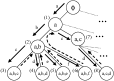
(b) Distance Ordering.

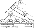
(c) Socio-Spatial Ordering.

Figure 2: Example of ordering strategies.

4.2 Pruning Strategies for SSGS

We also propose two pruning rules, namely Familiarity Pruning and Distance Pruning, which effectively filter out unqualified intermediate groups. The idea of Familiarity Pruning is to derive an upper bound on the number of acquaintances each member may have after new members are included into $S_{I}$. Similarly, Distance Pruning identifies a lower bound on the total spatial distance of each group grown from $S_{I}$. SSGS stops processing $S_{I}$ and backtracks if the current $S_{I}$ is pruned by Familiarity Pruning or Distance Pruning.

Familiarity Pruning. Specifically, the edges in any solution growing from $S_{I}$ can be divided into three categories: 1) $E_{I}$: the set of edges connecting any two vertices in $S_{I}$, 2) $E_{R}:$ the set of edges connecting any two vertices selected from $S_{R}$, and 3) $E_{IR}$: the set of edges connecting any two vertices in $S_{I}$ and the vertices selected from $S_{R}$. Apparently, $\left|E_{I}\right|=\frac{1}{2}\sum\nolimits_{v\in S_{I}}|N_{v}^{I}|$, where $N_{v}^{I}$ is the set of acquainted neighbors of $v$ in $S_{I}$. Since the selected vertices in $S_{R}$ are not clear, a good way is to find an upper bound on $\left|E_{R}\right|$, i.e., $\frac{1}{2}(p-|S_{I}|)\max_{v\in S_{R}}|N_{v}^{R}|$, where $N_{v}^{R}$ is the set of acquainted neighbors of $v$ in $S_{R}$. It is an upper bound because the vertex with the maximum degree in $S_{R}$ is identified, and $(p-|S_{I}|)$ vertices are selected from $S_{R}$. Similarly, an upper bound on $\left|E_{IR}\right|=\sum_{v\in S_{I}}|InterEdge(v)|$, where $InterEdge(v)$ is the set of edges connecting $v$ in $S_{I}$ to any vertices in $S_{R}$.

Notice that the number of edges in a feasible solution is half of the total degree of all the vertices in the solution. Therefore, with the above three categories of edges, Familiarity Pruning stops processing $S_{I}$ when the following condition holds,

$$\frac{1}{p}\left[\sum\nolimits_{v\in S_{I}}|N_{v}^{I}|+(p-|S_{I}|)\max_{v\in S_{R}}|N_{v}^{R}|\right.$$

$$\left.+2\cdot\sum_{v\in S_{I}}|InterEdge(v)|\right]<(p-k-1).\vspace{-12pt}$$ (2)

In the above inequality, the left-hand-side is an upper bound on the average number of attendees acquainted to each person in any feasible solution growing from $S_{I}$. The condition states that, on average, each attendee is acquainted with fewer than $p-k-1$ other attendees. Familiarity Pruning stops processing $S_{I}$ and backtracks if solutions growing from $S_{I}$ via the exploration of $S_{R}$ do not satisfy the familiarity constraint.

For the social graph in Figure 2(a) with $p=3$ and $k=0$, if $S_{I}=\{b,d\}$ and $S_{R}=\{e,f\}$, SSGS stops processing $S_{I}$ and backtracks because $\frac{1}{3}(0+1\cdot 1+2\cdot 1)=1<(3-0-1)=2$. In other words, moving any vertex from $S_{R}$ to $S_{I}$ will never generate a feasible solution following the familiarity constraint.

Distance Pruning. For a given $S_{I}$, $p-|S_{I}|$ vertices must be selected from $S_{R}$ to $S_{I}$. Apparently, further processing of $S_{I}$ is unnecessary if $S_{I}$ and the $p-|S_{I}|$ vertices with the shortest spatial distances to $q$ have a total distance larger than $D$, where $D$ is the best solution value obtained so far. Therefore, Distance Pruning identifies a lower bound and stops processing $S_{I}$ when the following condition holds,

$$\sum\nolimits_{u\in S_{I}}d_{u,q}+(p-|S_{I}|)d_{v_{\min},q}\geq D\vspace{-3pt}$$ (3)

where the first term is the total spatial distance from the vertices in $S_{I}$ to $q$. For $S_{R}$, only the vertex $v_{\min}$ with the smallest spatial distance to $q$ is accessed here, and $(p-|S_{I}|)d_{v_{\min},q}$ represents a lower bound on the total spatial distance for the above $p-|S_{I}|$ vertices in $S_{R}$.

Consider the social graph in Figure 2(a) with $p=3$ as an example. After a feasible solution $\{a,c,d\}$ is explored, its total spatial distance 27 is assigned to $D$. When SSGS considers $S_{I}=\{a,b\}$ and $S_{R}=\{e,f\}$, since $\sum\nolimits_{u\in S_{I}}d_{u,q}+(p-|S_{I}|)d_{v_{\min},q}=11+1\cdot 19=30>27$, Distance Pruning removes states $\{a,b,e\}$ and $\{a,b,f\}$, stops processing $S_{I}=\{a,b\}$, and backtracks to the previous state accordingly.

4.3 Heuristic Algorithm for SSGQ

As proved earlier, processing SSGQ is an NP-hard problem. In fact, even when the spatial distance is the same for every candidate, the problem is still NP-hard due to the familiarity constraint required to address. Therefore, in the following, we propose an efficient heuristic algorithm to obtain good solutions very efficiently. SSGS employs the branch-and-bound framework to incrementally improve the solution and find the optimal solution. A straightforward approach to develop heuristic algorithms for SSGQ is to stop the branch-and-bound search after the $i$-th feasible solution is obtained. However, it suffers two main drawbacks: 1) the running time is still not constrained in polynomial time, and 2) this approach only maintains the current minimal total spatial distance for solution space pruning but ignores the possibility to exploit many intermediate solutions to further improve the efficiency. To effectively address the above two issues, we propose an algorithm, named SSGMerge, which effectively utilizes the structures of intermediate solutions to generate a good feasible solution in polynomial time. The idea is to iteratively merge good socially tight groups with small spatial distances in different intermediate solutions obtained in earlier iterations.

Figure 3 presents a social network and a snapshot of the branch-and-bound tree with $p=4$, $k=1$, and $\theta=1$ for Socio-Spatial Ordering. After the first feasible solution $\{a,c,d,e\}$ is obtained, $\{a,d\}$ and $\{b,d\}$ are pruned accordingly by Distance Pruning, while $\{a,c,d,f\}$ and $\{a,c,e,f\}$ have higher total spatial distances than $\{a,c,d,e\}$. If the straightforward heuristic approach stops here, $\{a,b,c,d\}$ and $\{a,b,c,e\}$, both extending from $\{a,b\}$ and enjoying smaller total spatial distances, unfortunately are not to be discovered. In contrast, since $\{a,b,d\}$ and $\{a,c,d\}$ incurs small spatial distances, and if other candidates later join these two groups, they will become socially dense groups with small spatial distances. A promising idea is to merge the two groups into $\{a,b,c,d\}$ (similarly, merging $\{a,b,c\}$ and $\{a,c,e\}$ results into $\{a,b,c,e\}$). Based on this idea, we design a systematic approach to choose a set of suitable groups for constructing a good feasible solution.

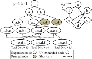
Figure 3: Example of SSGMerge.

The intermediate solutions expanded according to Socio-Spatial Ordering are created and tailored for each query with the specific parameters and the activity location. Therefore, it is more efficient for SSGMerge to process intermediate solutions directly. Given the group size $p$ of SSGQ, we maintain a set of $p$ intermediate solution queues $\{U_{1},...,U_{p}\}$, where each element in $U_{j}$ is an intermediate solution $S_{I}$ with $j$ attendees. To prioritize the intermediate solutions in $U_{|S_{I}|}$ with high social tightness and small spatial distance, we sort the intermediate solutions in $U_{|S_{I}|}$ with a ranking function $R(\cdot)$ based on Socio-Spatial Ordering,

$$R(S_{I})=p\cdot t\cdot\overline{\theta}+\sum_{v\in S_{I}}d_{v,q}$$

where $\overline{\theta}\geq k$ is set to the minimum $\theta$ that $S_{I}$ satisfies Socio-Spatial Ordering, and $d_{v,q}$ is the spatial distance from a candidate $v$ to the activity location $q$. The ranking function ranks $S_{I}$ based on its $\overline{\theta}$ value and the total spatial distance to $q$, and it gives a smaller score to the $S_{I}$ which has tighter social relationship and closer to $q$. Consider an example with the social graph shown in Figure 3. Assume $p=4$, $k=1$, $t=100$, $\overline{S}_{I}=\{a,b,c\}$, and $\widehat{S}_{I}=\{c,d,e\}$. Then, $R(\overline{S}_{I})=4\cdot 100\cdot 2+6=806$ while $R(\widehat{S}_{I})=4\cdot 100\cdot 1+12=412$. Therefore, SSGMerge is inclined to choose $\widehat{S}_{I}$.

TABLE I: Intermediate solutions maintained and constructed.

	Maintained and constructed solutions
$U_{1}$	$\{a\}$,$\{b\}$
$U_{2}$	$\{a,c\}$, $\mathbf{\{a,b\}}$
$U_{3}$	$\{a,c,d\}$,$\{a,c,e\}$,$\mathbf{\{a,b,c\}}$
$U_{4}$	$\{a,c,d,e\}$,$\mathbf{\{a,b,c,d\}}$,$\mathbf{\{a,b,c,e\}}$

Given the set of $p$ intermediate solution queues $\{U_{1},...,U_{p}\}$, the basic idea is to merge different pairs of small groups into larger ones. That is, for each $U_{i}$, we merge each pair of small intermediate groups $\widehat{S}_{I}$, $\overline{S}_{I}\in U_{i}$ into a new intermediate solution $\widetilde{S}_{I}$, i.e., $\widetilde{S}_{I}=\widehat{S}_{I}\cup\overline{S}_{I}$, and store $\widetilde{S}_{I}$ in the corresponding $U_{|\widetilde{S}_{I}|}$. If there are more than $\lambda$ intermediate solutions in $U_{i}$, after inserting merged intermediate solutions, $U_{i}$ maintains the $\lambda$ intermediate solutions with the smallest ranking value according to $R(\cdot)$. In other words, $\lambda$ here is a filtering parameter for controlling the quality and the number of the intermediate solutions in each $U_{i}$. Therefore, by first setting $i$ as $1$ and increasing $i$ by $1$ at each iteration, we can incrementally construct new intermediate solutions. Finally, we extract the feasible solution which incurs the minimum spatial distance from $U_{p}$ and return it as the solution.

More importantly, SSGMerge employs a pruning strategy to reduce the number of intermediate solutions under examination. When SSGMerge merges the intermediate solutions in $U_{i}$, an intermediate solution $\widehat{S}_{I}$ can be discarded if the following condition holds,

$$\sum_{v\in\widehat{S}_{I}}d_{v,q}+(p-|\widehat{S}_{I}|)\min_{i\leq j\leq p-1}\mu_{j}\geq D.$$

In the above condition, $\mu_{j}$ is the minimum spatial distance of the candidates existing in $U_{j}$, and $D$ is the currently best solution value. It measures the minimum increment of the spatial distance of $\widehat{S}_{I}$ when $\widehat{S}_{I}$ is merged with others and becomes a feasible solution. If this condition holds, any feasible solution expanded from $\widehat{S}_{I}$ (i.e., having $\widehat{S}_{I}$ as a subset), will never become a better solution, and thus $\widehat{S}_{I}$ can be safely discarded.

In Table I, the merged solutions constructed by SSGMerge are shown in bold with underscores. For example, $\{a,b\}$ is constructed by merging $\{a\}$ and $\{b\}$ in $U_{1}$, and $\{a,b,c,d\}$ can be constructed by merging $\{a,c,d\}$ and $\{a,b,c\}$ in $U_{3}$, where $\{a,b,c\}$ is the combination of $\{a,c\}$ and $\{a,b\}$ in $U_{2}$. After the merging process is completed, we extract the feasible solution with the minimum spatial distance from $U_{p}$, i.e., $U_{4}$ in Table I, which is $\{a,b,c,d\}$. As compared to the best feasible solution $\{a,c,d,e\}$ obtained in Figure 3, the total spatial distance of $\{a,b,c,d\}$ is $10$, which is smaller than that of $\{a,c,d,e\}$, i.e., $13$.

SSGMerge involves two parameters, $w$ and $\lambda$, and terminates the search process after $w$ states have been generated in the branch-and-bound tree. SSGMerge then refines the solutions with the above merge approach. By effectively restricting the number of generated intermediate solutions, SSGMerge can efficiently construct a good feasible solution according to the following theorem.

Theorem 3

The running time of SSGMerge is $O(p\lambda^{2}\log p\lambda+wp^{2}+|V|(\log|V|)^{2})$.

Proof 3

SSGMerge first generates $w$ nodes in the branch-and-bound tree before it merges those intermediate solutions and creates feasible solutions. Three operations are performed: 1) Socio-Spatial Ordering, 2) Distance Pruning, and 3) Familiarity Pruning. Socio-Spatial Ordering includes Distance Ordering and the checking of Eq. (1) in Section 4.1. Distance browsing strategy, i.e., iteratively extracting the candidate attendee with the minimum spatial distance to $q$ from R-Tree, in Distance Ordering is performed $w$ times. Therefore, in the worst case, the number of R-Tree leaf node access is $O(|V|)$, and the traversal from the root to a leaf node of R-Tree incurs $O(\log|V|)$ R-Tree internal node access. Since each R-Tree node access incurs $O(1)$ time for distance computation, the time of R-Tree node access is $O(|V|\log|V|)$. The priority queue maintained for Distance Ordering takes $O(\log s)$ time for each insertion and deletion operation, where $s$ is the size of the priority queue. Since there are $O(|V|\log|V|)$ elements inserted into the priority queue, and the insertion cost of each element is $O(\log(|V|\log|V|))$ (in worst case, the size of the priority queue is $O(|V|\log|V|)$). Therefore, the total cost is $O(|V|\log|V|)\cdot O(\log(|V|\log|V|))=O(|V|(\log|V|)^{2})$.

For checking Eq. (1) of Socio-Spatial Ordering, since the size of $S_{I}$ does not exceed $p$, it requires $O(p^{2})$ time to compute $F(S_{I}\cup\{v\})$ for each examination, i.e., examining if a vertex ${v}$ can be included in the current $S_{I}$. Therefore, checking Eq. (1) for $w$ times takes $O(wp^{2})$ time.

Familiarity Pruning is performed in $O(wp^{2})$ time for $w$ examinations. Distance Pruning at each time examines the first element of the priority queue and the total spatial distance in $S_{I}$ with $O(p)$ time. Therefore, Distance Pruning takes $O(wp)$ time for $w$ examinations in the branch-and-bound tree. In summary, the time complexity of $w$ attempts for including a node into $S_{I}$ is $O(wp^{2})+O(wp)+O(|V|(\log|V|)^{2})=O(wp^{2}+|V|(\log|V|)^{2})$.

On the other hand, when SSGMerge merges intermediate solutions, at each $U_{i}$, it first ranks the intermediate solutions in $U_{i}$ with the ranking function and then discards those with ranks higher than $\lambda$. This step takes $O(p\lambda^{2}\log p\lambda)$ time because in the worst case, each merged intermediate solution in $U_{i},$ $1\leq i\leq j$ is inserted into $U_{j}$. It costs $O(\lambda^{2})$ time for SSGMerge to combine each pair of intermediate solutions within each $U_{i}$ for $1\leq i\leq p$, including checking the pruning condition. Therefore, it takes $O(p\lambda^{2})$ time for merging the intermediate solutions. Overall, the running time for SSGMerge is $O(p\lambda^{2}\log p\lambda+wp^{2}+|V|(\log|V|)^{2})$.

Please note that $|V|$ in the complexity comes from the worst case of R-Tree distance browsing. However, with the assumption of uniform distribution of the candidates’ locations, the expected time of R-Tree distance browsing becomes $O(w\log|V|\cdot\log(w\log|V|))$. More importantly, the experimental results manifest that SSGMerge is much faster than SSGS because SSGMerge effectively merges intermediate solutions into good feasible solutions to avoid examining the large search space.

5 Algorithm Design for MRGQ

In this section, we turn our attention to Multiple Rally-Point Social Spatial Group Query (MRGQ), which finds 1) the most suitable activity location from a set of candidate locations and 2) a socially acquainted group with the minimal total spatial distance to the activity location. More specifically, MRGQ aims to find a pair $\langle F,q^{*}\rangle$, where $F$ is a socially acquainted group of $p$ people satisfying the familiarity constraint, and $q^{*}\in Q$ is a location in $Q$ such that $\langle F,q^{*}\rangle$ incurs the minimum total spatial distance. MRGQ is more difficult than SSGQ since different candidate social groups are closer to different locations, which need to be carefully considered as well.

To address the issue of multiple candidate locations, a straightforward approach is to repeat the SSGS algorithm $|Q|$ times to sequentially find the best group for each location. Nevertheless, this straightforward approach is not efficient because a spatial correlation may exist among multiple activity locations and thus can be exploited. In addition, it is desirable to design some effective index structures to facilitate efficient traversal and pruning of the search space. In this work, we propose to index the candidates with an R-Tree, while indexing the activity locations with a BallTree [14]. Accordingly, we design new ordering strategies to quickly identify an activity location near an intermediate group of candidates satisfying the familiarity constraint and pruning strategies to avoid generating redundant $\langle\widehat{F},q_{i}\rangle$ pairs, where $\widehat{F}$ is a group of $p$ candidates satisfying the familiarity constraint. Moreover, two effective strategies for traversing the search space are proposed, including All-Pair Distance Ordering and Single-Reference Distance Ordering. Processing time is also improved by introducing a number of new search space pruning rules, including Inner-Triangle Distance Pruning, Outer-Triangle Distance Pruning, and Activity Location Distance Pruning. In summary, during the process of selecting attendees and an activity location, we exploit both the spatial distances among different candidate locations as well as the distances from attendees to activity locations to effectively prune redundant search space to efficiently find the optimal solution.

In Section 2, we present an Integer Linear Programming (ILP) formulation for MRGQ which can obtain an optimal solution via a commercial solver, such as the IBM CPLEX [1] parallel optimizer, one of the fastest commercial parallel solvers. However, as shown in Section 7, this still requires an unacceptable amount of time to find the optimal solution because MRGQ needs to simultaneously process the spatial and social dimensions. Therefore, in Section 5.2, we design a new algorithm to efficiently process MRGQ.

5.1 Baseline Algorithms for MRGQ

The baseline algorithms are extensions of SSGS mentioned in Section 4. While Socio-Spatial Ordering and Distance Pruning remain the same, we extend Familiarity Pruning introduced in Section 4.2 to tailor the familiarity constraint for MRGQ. Specifically, if one of the following conditions holds, Familiarity Pruning stops moving any candidates into $S_{I}$, and the algorithm backtracks to the previous step to consider other candidate attendees.

$$|S_{I}|-\min_{v\in S_{I}}|N_{v}\cap S_{I}|>k+1\text{, or}$$ (4)

$$\sum_{v\in S_{R}}|S_{R}\cap N_{v}|<(p-|S_{I}|)(p-|S_{I}|-k-1),$$ (5)

where $N_{v}$ is the set of neighbors of $v$ in $V$.

In Eq. (4), $\min_{v\in S_{I}}|N_{v}\cap S_{I}|$ represents the minimum number of neighbors for each individual $v$ in $S_{I}$. In other words, $|S_{I}|-\min_{v\in S_{I}}|N_{v}\cap S_{I}|-1$ is the maximum number of unacquainted members for $v$ in $S_{I}$, and $-1$ is incorporated above to exclude $v$ herself. If $|S_{I}|-\min_{v\in S_{I}}|N_{v}\cap S_{I}|-1>k$, at least one individual in $S_{I}$ has more than $k$ unacquainted members in $S_{I}$. This situation violates the familiarity constraint. Therefore, the pruning strategy holds since any group growing from the current $S_{I}$ will never satisfy the familiarity constraint.

Eq. (4) considers the vertex degrees of the individuals in $S_{I}$. In contrast, the pruning condition specified in Eq. (5) considers the degrees of the individuals that have not been moved into $S_{I}$, i.e., those individuals that are in $S_{R}$. In the right-hand-side (RHS) of Eq. (5), $(p-|S_{I}|)$ is the number of individuals that need to be moved from $S_{R}$ to $S_{I}$. On the other hand, for any solution group that satisfies the familiarity constraint, the degree of each member is at least $(p-k-1)$ in the group. Therefore, if $S_{R}$ has an individual $u$ with the number of neighbors in $S_{R}$ smaller than $(p-|S_{I}|-k-1)$, $S_{I}$ will never grow into a feasible solution when $u$ is selected into $S_{I}$. In other words, if the total number of neighbors that all individuals in $S_{R}$ have (i.e., $\sum_{v\in S_{R}}|S_{R}\cap N_{v}|$) is smaller than $(p-|S_{I}|)(p-|S_{I}|-k-1)$, selecting any $(p-|S_{I}|)$ individuals from $S_{R}$ into $S_{I}$ will never generate a feasible solution, and thus this intermediate group can be trimmed accordingly.

For example, if $p=4$, $k=0$ and the social graph is shown in Figure 2(a). If $S_{I}=\{a,e\}$, then this $S_{I}$ can be pruned by Eq. (4) since $2-0>0+1$ holds, i.e., at least one vertex in current $S_{I}$ does not have enough friends to satisfy the familiarity constraint. Similarly, if $p=5,k=0$ and $S_{I}=\{a\}$, $S_{R}=\{b,c,d,e,f\}$, $S_{I}$ can also be pruned by Eq. (5) because $1+2+1+3+1<(5-1)(5-1-0-1)$ holds, i.e., the candidates in $S_{R}$ do not provide sufficient social tightness for the current $S_{I}$ to satisfy the familiarity constraint.

In the following, we introduce two baseline algorithms, namely SSP and SFGP.

Sequential SSGQ Processing (SSP). As discussed earlier, an intuitive approach for answering MRGQ is to sequentially invoke algorithm SSGS for each activity location. However, even though the intermediate best solution can be exploited to prune inferior solutions not yet examined, this approach still incurs a huge query processing cost because it does not simultaneously trim multiple activity locations. Therefore, we improve SSP to SFGP as follows.

Sequential Feasible Groups Processing (SFGP). In contrast to SSP that sequentially explores $|Q|$ branch-and-bound trees (i.e., one for each activity location), SFGP constructs only one branch-and-bound tree to facilitate joint exploration of the spatial and social dimensions. In addition to $S_{I}$ and $S_{R}$, for each node in the tree, SFGP also maintains a set $Q_{I}$ of remaining activity locations that need to be explored. Initially, setting $S_{I}=\varnothing$, $S_{R}=V$, and $Q_{I}=Q$, SFGP first finds a reference activity location $q_{ref}\in Q_{I}$ to guide the exploration, where $q_{ref}$ is the closest location to a candidate attendee $u\in S_{R}$ (i.e., $q_{ref}$ and $u$ are the spatially closest pair). As such, $q_{ref}$ can lead to a smaller total spatial distance in early stages of SFGP. Afterwards, SFGP moves candidates from $S_{R}$ into $S_{I}$ according to Socio-Spatial Ordering (introduced in Section 4.1) based on $q_{ref}$. After moving a candidate from $S_{R}$ into $S_{I}$, SFGP determines whether $S_{I}$ can be pruned by Familiarity Pruning mentioned in Eqs. (4) and (5). If $S_{I}$ is pruned by Familiarity Pruning, SFGP stops moving candidates into the current $S_{I}$ and backtracks because the current $S_{I}$ cannot grow into any feasible solutions. Moreover, each time a candidate is moved into $S_{I}$, SFGP examines each activity location $q_{i}\in Q_{I}$ with the Distance Pruning condition (introduced in Section 4.2). An activity location $q_{i}$ will be removed from $Q_{I}$ if it is distant from most members in $S_{I}$ (i.e., $q_{i}$ is pruned by Distance Pruning). While expanding $S_{I}$, if $Q_{I}$ becomes empty (i.e., all activity locations in $Q_{I}$ are pruned), SFGP stops the expansion and backtracks.

When $S_{I}$ contains exactly $p$ candidates and satisfies the familiarity constraint, SFGP computes the spatial distances from $S_{I}$ to each activity location in $Q_{I}$, and extracts the activity location $q\in Q_{I}$ which incurs the minimum spatial distance to $S_{I}$. If the spatial distance from $S_{I}$ to $q$ is smaller than the current minimum distance $D$, SFGP records $\left\langle S_{I},q\right\rangle$, updates $D$ and backtracks to examine other possible solutions. When the search space is explored, SFGP outputs the recorded best solution and the corresponding activity location.

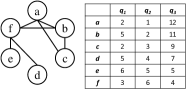
(a) Social graph and spatial distances.

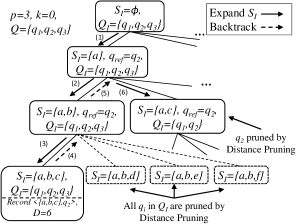
(b) Branch-and-bound tree of SFGP.

Figure 4: Example of SFGP.

Figure 4(b) presents an example of SFGP to show that the size of $Q_{I}$ can rapidly decrease when a few more candidates are moved into $S_{I}$. The social network and the corresponding spatial distances to each $q_{i}\in Q_{I}$ are shown in Figure 4(a). Assume $p=3$ and $k=0$, at the beginning, $S_{I}=\varnothing$, $Q_{I}=\{q_{1},q_{2},q_{3}\}$ and $S_{R}=V$. In step (1), SFGP first identifies $q_{ref}=q_{2}$ because $q_{2}$ and candidate attendee $a$ are the spatially closest pair while $a\in S_{R}$, and then SFGP moves $a$ from $S_{R}$ into $S_{I}$. In step (2), SFGP moves $b$ from $S_{R}$ into $S_{I}$. Note that $b$ is the candidate attendee in $S_{R}$ who is closest to $q_{ref}$. Here, moving $b$ into $S_{I}$ follows Socio-Spatial Ordering (SSO), and $S_{I}\cup\{b\}$ is not pruned by Familiarity Pruning. In step (3), SFGP moves $c$ into $S_{I}$ where $S_{I}=\{a,b,c\}$ satisfies the familiarity constraint. SFGP then scans over the activity locations in $Q_{I}$ and extracts $q_{2}$ because $q_{2}$ incurs the minimum total spatial distance to $S_{I}$. SFGP updates the currently best solution $\left\langle\{a,b,c\},q_{2}\right\rangle$ and its distance value (i.e., $D=6$) and backtracks to the previous state as step (4), i.e., $S_{I}=\{a,b\}$ and $Q_{I}=\{q_{1},q_{2},q_{3}\}$. SFGP then discovers that by applying Distance Pruning, all the activity locations in $Q_{I}$ can be removed, i.e., moving $d$, $e$ and $f$ into $S_{I}$ does not generate a better solution. Therefore, SFGP stops expanding the current $S_{I}$ and backtracks through step (5). Now, $S_{I}=\{a\}$ and SFGP moves $c$ into $S_{I}$ in step (6). In this case, $q_{3}$ can be removed from $Q_{I}$ because Distance Pruning indicates that $q_{3}$ will never lead to any better solutions given the current $S_{I}$. Therefore, SFGP only needs to examine $q_{1}$ and $q_{2}$ in the future expansion of the current $S_{I}$. During the process, if SFGP finds a feasible solution with a distance better than $D$, it records the solution and update $D$. SFGP repeats the above procedures and returns the best solution after the search is complete.

As compared to SSP, SFGP jointly examines the activity locations and candidate attendees, and employs Distance Pruning to effectively remove the activity locations that do not lead to better solutions. It then utilizes Familiarity Pruning to discard the intermediate groups that cannot grow into feasible solutions. Moreover, SFGP avoids the repeated explorations of different social groups, i.e., the same social group may be generated and examined for $|Q|$ times in SSP. As shown in Section 7, SFGP outperforms SSP. However, after carefully examining SFGP, we still find a number of areas that can be further improved, and thus propose a more efficient algorithm as detailed below.

5.2 Algorithm MAGS for MRGQ

Although SFGP is able to prune redundant activity locations, it relies on sequential scans over $Q_{I}$ to determine whether a location in $Q_{I}$ can be safely pruned. Therefore, for every $q_{i}$ in $Q_{I}$, SFGP has to calculate a lower bound on the total spatial distance of the feasible solution generated from $S_{I}$ and $q_{i}$ according to Distance Pruning. On the other hand, identifying $q_{ref}$ needs a scan over the activity locations in $Q_{I}$. Moreover, the selected $q_{ref}$ may not always be good because SFGP decides $q_{ref}$ before the first candidate attendee is moved into $S_{I}$, instead of adaptively changing $q_{ref}$ as $S_{I}$ grows.

To address these issues, we propose an algorithm, namely Multiple Activity-Location Group Selection (MAGS), to efficiently process MRGQ. Similar to SFGP, MAGS processes multiple activity locations simultaneously. However, MAGS incorporates the following new ideas: a) an index of activity locations, b) new distance ordering strategies, including Single-Reference Distance Ordering and All-Pair Distance Ordering, and c) new distance pruning strategies, including Activity Location Distance Pruning, Outer-Triangle Distance Pruning and Inner-Triangle Distance Pruning. Using an index for the activity locations avoids sequential scans of the activity locations in $Q_{I}$ (i.e., for the selection of $q_{ref}$ and pruning of unnecessary locations). The new distance ordering strategies obtain $q_{ref}$ more efficiently and enable $q_{ref}$ to change during the expansion of $S_{I}$. As a result, feasible solutions with smaller total spatial distances can be obtained more effectively. Moreover, the new distance pruning strategies exploit the interplay between $S_{I}$ and the activity locations, as well as the mutual distances of different locations, to effectively and simultaneously prune multiple activity locations.

5.3 Indexing the Activity Locations

As previously mentioned, SFGP incurs many sequential scans over the activity locations due to Distance Pruning, i.e., each time a candidate is moved into $S_{I}$, $Q_{I}$ needs to be scanned to determine whether some activity locations can be pruned. Moreover, as SFGP extracts $q_{ref}\in Q_{I}$ and $u\in S_{R}$ at the beginning, $q_{ref}$ is not always the closest activity location for $S_{I}$ to be expanded afterward, especially when $S_{I}$ does not include $u$. Therefore, the proposed All-Pair Distance Ordering (APDO) is designed to dynamically select $q_{ref}\in Q_{I}$ and $u\in S_{R}$ according to the current $S_{I}$ (as described in Section 5.4). More specifically, the next attendee $u$ that will be moved to $S_{I}$ and the corresponding $q_{ref}$ need to minimize the total spatial distance from $S_{I}\cup\{u\}$ to $q_{ref}$, i.e., $\min_{u\in S_{R},q_{ref}\in Q_{I}}\left\{d_{u,q_{ref}}+\sum_{v\in S_{I}}d_{v,q_{ref}}\right\}$. Equipped with APDO, MAGS finds good feasible solutions more quickly and prunes search space with distance pruning strategies. However, this approach needs $O(|V|)$ sequential scans over $Q_{I}$ before a new candidate attendee is identified and moved into $S_{I}$.

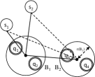
(a) Indexed with balls.

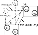
(b) Indexed with MBRs.

Figure 5: Comparisons of R-Tree and BallTree.

One way to avoid sequential scans over $Q_{I}$ is to index the activity locations in an index structure. This may facilitate rapid estimation of the spatial distances from activity candidates to potential activity locations and thus allow distance pruning strategies to immediately remove redundant activity locations from $Q_{I}$. With such an index structure, triangular inequality may be exploited in distance pruning strategies to further reduce distance computations (detailed later). Although the index structure has to be constructed at runtime, it can be reused many times in query processing.

We adopt BallTree [14] to index the activity locations. In BallTree, each activity location $q_{i}\in Q$ is stored as a leaf node, and each internal node in BallTree is the smallest ball covering all the children balls. Here, a ball $B$ is associated with its center $ctr(B)$ and radius $r(B)$. The distance lower bound from a candidate $u$ to a ball $B$ on 2D space can be computed as $MINDIST(u,B)=d_{u,ctr(B)}-r(B)$. The leaves of the BallTree are the activity locations, while the internal nodes in the tree corresponds to a ball containing multiple activity locations.

BallTree enables the removal of many unqualified locations at once, as illustrated in Figure 5(a). To simultaneously explore and prune multiple activity locations, a lower bound on the total spatial distance from $S_{I}=\{s_{1},s_{2}\}$ to a ball, e.g., $B_{1}$, can be derived. If this distance lower bound exceeds the currently best solution value $D$, it assures that no activity location in $B_{1}$ will produce a better solution with any social group grown from $S_{I}$. Thus, all activity locations in $B_{1}$ can be safely pruned. In Figure 5(a), $\sum_{s_{i}\in S_{I}}MINDIST(s_{i},B_{1})$ serves as a lower bound on the total spatial distance from $S_{I}$ to $q_{1}$ and $q_{2}$. Moreover, we can employ triangular inequality to avoid the distance computation of $\sum_{s_{i}\in S_{I}}MINDIST(s_{i},B_{2})$, i.e., $\sum_{s_{i}\in S_{I}}MINDIST(s_{i},B_{2})=\sum_{s_{i}\in S_{I}}(d_{s_{i},ctr(B_{2})}-r(B_{2}))<|S_{I}|\cdot d_{ctr(B_{1}),ctr(B_{2})}+\sum_{s_{i}\in S_{I}}d_{s_{i},ctr(B_{1})}-|S_{I}|\cdot r(B_{2})$. Therefore, only the distance from $ctr(B_{1})$ to $ctr(B_{2})$ needs to be computed, together with $\sum_{s_{i}\in S_{I}}d_{s_{i},ctr(B_{1})}$, to derive a lower bound on the spatial distance from $S_{I}$ to $B_{2}$. In summary, instead of invoking sequential scans which need $|S_{I}|\cdot m$ distance computations to find the total spatial distances from $S_{I}$ to $m$ activity locations, indexing activity locations in BallTree requires only $|S_{I}|+(n-1)$ distance computations, where $n$ is the number of balls.

An alternative index is R-Tree, but we argue that BallTree is more suitable for indexing activity locations here. Figure 5(b) illustrates an example where the activity locations are indexed in an R-Tree. As shown, minimum bounding rectangles (MBRs) are used to provide boundary information over locations inside them. In Figure 5(b), $\sum_{s_{i}\in S_{I}}MINDIST(s_{i},M_{1})$ serves as a lower bound on the total spatial distance from $S_{I}$ to $q_{1}$ and $q_{2}$, where $MINDIST(s_{i},M_{1})$ denotes the minimum distance from $s_{i}$ to MBR $M_{1}$. However, it is difficult to employ triangular inequality with R-Tree to quickly obtain a lower bound on $\sum_{s_{i}\in S_{I}}MINDIST(s_{i},M_{2})$. As shown in Figure 5(b), where $MINDIST(s_{1},M_{1})+x>MINDIST(s_{1},M_{2})$ holds, the inequality $MINDIST(s_{1},M_{1})+MINDIST(M_{1},M_{2})>MINDIST(s_{1},M_{2})$ is not guaranteed to hold because $MINDIST(M_{1},M_{2})\leq x$. Therefore, it is necessary to compute $MINDIST(s_{1},M_{2})$ and $MINDIST(s_{2},M_{2})$ directly, incurring $|S_{I}|\cdot\hat{n}$ on-line distance computations to derive all lower bounds, where $\hat{n}$ is the number of MBRs. In contrast, BallTree needs only $|S_{I}|+(n-1)$ distance computations with $n$ balls. Therefore, BallTree is preferable to R-Tree in our MAGS design.

BallTree brings two advantages to MAGS: 1) BallTree enables the design of efficient distance ordering strategies. By traversing both R-Tree (for indexing candidate attendees) and BallTree (for indexing activity locations), our proposed distance ordering strategies avoid redundant examinations of candidate attendees and activity locations to extract the reference activity location $q_{ref}$. The new distance ordering strategies, combined with the original Socio-Spatial Ordering mentioned in Section 4.1, are promising to find good feasible solutions quickly and prune redundant search space effectively. 2) BallTree enables distance-based pruning of activity locations at once in the early stages. Moreover, the lower bound on the total spatial distance from a set of balls to $S_{I}$ can be quickly obtained to facilitate pruning. In the following, we first propose two distance ordering strategies and then introduce the distance pruning strategies based on R-Tree and BallTree.

5.4 Distance Ordering

While Socio-Spatial Ordering in SSGS is applicable to MAGS, its design does not consider selections of activity locations. Here we propose two new distance ordering strategies for MAGS: (1) Single-Reference Distance Ordering (SRDO). It selects the activity location along with the first candidate attendee, $v_{seed}$, for $S_{I}$. Note that the total spatial distance of the feasible solutions obtained by SRDO may not be minimal since only a single location $q_{ref}$ is fixed as a reference. (2) All-Pair Distance Ordering (APDO). It adaptively changes the optimal activity location according to different $S_{I}$, and always chooses the best activity location when a new attendee is included into $S_{I}$ to minimize the total spatial distance from $S_{I}$ to the new reference activity location $q_{ref}$.

Single-Reference Distance Ordering (SRDO). At the beginning, i.e., $S_{I}=\varnothing$, SRDO starts by selecting a seed candidate $v_{seed}$ and a reference activity location $q_{ref}$ such that $d_{v_{seed},q_{ref}}$ is minimal. However, to avoid excessive distance computations, we fix $q_{ref}$ as $S_{I}$ grows. While SRDO requires later examination of other activity locations, the minimized distance may effectively eliminate consideration of many potential activity locations. To efficiently obtain $v_{seed}$ and $q_{ref}$, we traverse R-Tree (indexing the candidate attendees) and BallTree (indexing activity locations) simultaneously, to reduce the number of distance computations. To further improve the efficiency, a distance lower bound from any candidate within an MBR $M_{i}$ to any activity location within a ball $B_{j}$, $MINDIST(M_{i},B_{j})$, is derived as $MINDIST(M_{i},B_{j})=MINDIST(M_{i},ctr(B_{j}))-r(B_{j})$, where $MINDIST(M_{i},ctr(B_{j}))$ is the minimum distance from $M_{i}$ to the center of $B_{j}$, and $r(B_{j})$ is the radius of $B_{j}$. $MINDIST(M_{i},B_{j})$ represents a distance lower bound from any candidate within $M_{i}$ to any activity location in $B_{j}$, which is particularly useful to determine redundant examinations of candidate attendees and activity locations located in distant MBRs and balls in R-Tree and BallTree.

More specifically, SRDO maintains two lists, $U_{R}$ and $U_{B}$, to record the traversal status of R-Tree and BallTree. Initially, we insert the root of R-Tree into $U_{R}$ and the root of BallTree into $U_{B}$. Then, at each stage, we find the MBR $M_{i}$ in $U_{R}$ and the ball $B_{j}$ in $U_{B}$ that incur the minimum $MINDIST(M_{i},B_{j})$. If $M_{i}$ is not a leaf node in R-Tree, we pop $M_{i}$ from $U_{R}$ and insert its children back into $U_{R}$, while a non-leaf node in BallTree is performed similarly. If the extracted $M_{i}$ and $B_{j}$ are both leaf nodes, they are assigned as $v_{seed}$ and $q_{ref}$, respectively. Note that the entries in $U_{R}$ and $U_{B}$ are popped in accordance with the shortest distance between them, $v_{seed}$ and $q_{ref}$ are indeed the closet attendee-location pair. Each candidate attendee $v_{i}$ and activity location $q_{j}$ in any other MBR $M_{i}$ and ball $B_{j}$ must incur a larger spatial distance since $MINDIST(M_{i},B_{j})$ is a lower bound, and $d_{v_{seed},q_{ref}}\leq MINDIST(M_{i},B_{j})\leq d_{v_{i},q_{j}}$. Therefore, this approach effectively avoids examining attendees and locations that are mutually distant because their corresponding MBRs and balls will never be extracted from the lists. Moreover, if $d_{v_{seed},q_{ref}}>t$ (where $t$ is the spatial radius), MAGS can stop since there is no feasible solution in this case.

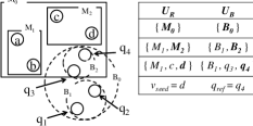
Figure 6: Example of SRDO.

Figure 6 presents an illustrative example for SRDO. Assume there are four candidates $\{a,b,c,d\}$ indexed by an R-Tree and four activity locations $\{q_{1},q_{2},q_{3},q_{4}\}$ indexed by a BallTree. To find $v_{seed}$ and $q_{ref}$, we first insert the root of R-Tree, $M_{0}$, into $U_{R}$, and insert the root of BallTree, $B_{0}$, into $U_{B}$. There is only one element in each list, and $MINDIST(M_{0},B_{0})=0$ since they overlap. Thus, SRDO extracts $M_{0}$ and $B_{0}$ and insert their children into $U_{R}$ and $U_{B}$, respectively. Now, $U_{R}=\{M_{1},M_{2}\}$ and $U_{B}=\{B_{1},B_{2}\}$. SRDO then extracts $M_{2}$ and $B_{2}$ from each list since $MINDIST(M_{2},B_{2})$ is the smallest one. Afterwards, we insert the children of $M_{2}$ and $B_{2}$ into the lists, respectively, and now $U_{R}=\{M_{1},c,d\}$ and $U_{B}=\{B_{1},q_{3},q_{4}\}$. SRDO finds that $d$ and $q_{4}$ incur the minimum spatial distance and assigns $v_{seed}$ as $d$ and $q_{ref}$ as $q_{4}$.

Once $v_{seed}$ and $q_{ref}$ are extracted, $q_{ref}$ in SRDO is fixed. The candidate attendees chosen later still need to follow Socio-Spatial Ordering to maintain the required social tightness of $S_{I}$, and Familiarity Pruning is employed to prune the intermediate solutions that will not become feasible groups. Moreover, distance pruning strategies based on R-Tree and BallTree are employed to remove activity locations (detailed later) that will never produce a better solution.

All-Pair Distance Ordering (APDO). With SRDO, as $S_{I}$ grows, the $q_{ref}$ selected initially may not be the eventual activity location with the minimum total distance to $S_{I}$. Figure 7 presents an illustrative example with $p=3$ and $\{a,b,c,d\}$ as the candidates indexed by R-Tree, while $\{q_{1},q_{2},q_{3},q_{4}\}$ are activity locations indexed by BallTree. SRDO finds $d$ for $v_{seed}$ and $q_{4}$ for $q_{ref}$. Thereafter, $a$ and $c$ are moved into $S_{I}$. However, since $a$ and $c$ are distant from $q_{4}$, the solution obtained by SRDO, i.e., $\left\langle\{a,c,d\},q_{4}\right\rangle$, incurs a large total spatial distance. In contrast, a better feasible solution is $\left\langle\{a,b,d\},q_{3}\right\rangle$, which greatly reduces the total spatial distance. Therefore, we propose All-Pair Distance Ordering (APDO), to select proper candidates from $S_{R}$ and adaptively switch $q_{ref}$ to the most suitable activity location.

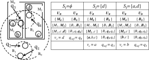
Figure 7: Example of APDO.

We propose All-Pair Distance Ordering (APDO) to select proper candidates from $S_{R}$ and adaptively switch $q_{ref}$ to the most suitable activity location. More specifically, APDO simultaneously chooses $q_{ref}$ and a candidate attendee $v_{c}$ to expand $S_{I}$ at each iteration, such that the total spatial distance from $S_{I}$ to the selected $q_{ref}$ is minimized, i.e.,

$$\min_{v_{c}\in S_{R},q_{ref}\in Q_{I}}\left\{d_{v_{c},q_{ref}}+\sum_{v\in S_{I}}d_{v,q_{ref}}\right\}.\vspace{-5pt}$$ (6)

A straightforward approach to select $v_{c}$ and $q_{ref}$ is to scan over the entire sets of $S_{R}$ and $Q_{I}$. However, this approach requires $\left(|S_{R}|+|S_{I}|\right)\cdot|Q_{I}|$ distance computations when we move a candidate into $S_{I}$. To reduce this overhead, we traverse both R-Tree and BallTree simultaneously, to reduce unnecessary distance computations.

Two lists $U_{R}$ and $U_{B}$ are maintained during the traversal of R-Tree and BallTree. At each stage, MBR $M_{i}$ and ball $B_{j}$ are extracted from $U_{R}$ and $U_{B}$ based on the following score function.

$$\min_{M_{i}\in U_{R},B_{j}\in U_{B}}\left\{\sum_{v\in S_{I}}MINDIST(v,B_{j})+\right.$$

$$\left.MINDIST(M_{i},B_{j})\right\}$$ (7)

where $MINDIST(v,B_{j})=d_{v,ctr(B_{j})}-r(B_{j})$ and $MINDIST(M_{i},B_{j})$ cannot exceed $t$. In Eq. (7), the first term represents the minimum total spatial distance from $S_{I}$ to any activity location within $B_{j}$, while the second term represents the minimum spatial distance from a candidate attendee in $M_{i}$ to an activity location in $B_{j}$.

After extracting $M_{i}$ and $B_{j}$ from Eq. (7), if $M_{i}$ is not a leaf node on R-Tree, we pop it from $U_{R}$ and insert its children into $U_{R}$. Similarly, if $B_{j}$ is a non-leaf node on BallTree, we also pop it from $U_{B}$ and insert its children into $U_{B}$. As such, APDO extracts $v_{c}$ and $q_{ref}$ without accessing the candidate attendees and activity locations distant from each other. We repeat the above procedure until $M_{i}$ and $B_{j}$ are both leaf nodes and $M_{i}\in S_{R}$. Finally, we move $v_{c}$ from $S_{R}$ into $S_{I}$ and continue the branch-and-bound search. Moreover, during the above procedure, if $MINDIST(v_{c},B_{i})>t$ for a ball $B_{i}$, all the activity locations within $B_{i}$ can be removed from $Q_{I}$ since no activity locations in $B_{i}$ satisfies the spatial radius constraint. APDO iteratively extracts $v_{c}$ and $q_{ref}$ which incur the minimum spatial distance so as to avoid the situation where $q_{ref}$ is only close to a small number of candidate attendees but distant from the others. Moreover, APDO also allows for the early pruning of activity locations that are distant from the candidate attendees. This effectively reduces computation overhead when performing distance pruning strategies afterwards.

Figure 7 presents an example with four candidates $\{a,b,c,d\}$ indexed by R-Tree and four activity locations $\{q_{1},q_{2},q_{3},q_{4}\}$ indexed by BallTree. Initially, when $S_{I}=\varnothing$, APDO finds the first $v_{c}$ and the corresponding $q_{ref}$ as follows (see the first column in the table). APDO first inserts the root of R-Tree, $M_{0}$, into $U_{R}$, and inserts the root of BallTree, $B_{0}$, into $U_{B}$. There is only one element in each list, and $MINDIST(M_{0},B_{0})=0$ since they overlap. Thus, APDO extracts $M_{0}$ and $B_{0}$ and inserts their children into $U_{R}$ and $U_{B}$, respectively. Now, $U_{R}=\{M_{1},M_{2}\}$ and $U_{B}=\{B_{1},B_{2}\}$. APDO then extracts $M_{2}$ and $B_{2}$ from each list since $MINDIST(M_{2},B_{2})$ is the smallest one. Afterwards, we insert the children of $M_{2}$ and $B_{2}$ into the lists, respectively, and now $U_{R}=\{M_{1},c,d\}$ and $U_{B}=\{B_{1},q_{3},q_{4}\}$. APDO finds that $d$ and $q_{4}$ incur the minimum spatial distance, and the first candidate to be moved into $S_{I}$ is $d$ with the corresponding $q_{ref}$ as $q_{4}$.

To choose the second candidate $v_{c}$ and update $q_{ref}$ (see the second column in the table), we insert the roots $M_{0}$ and $B_{0}$ of the R-Tree and BallTree into $U_{R}$ and $U_{B}$, respectively. Then $M_{0}$ and $B_{0}$ are extracted to insert their children, i.e., $U_{R}=\{M_{1},M_{2}\}$ and $U_{B}=\{B_{1},B_{2}\}$. Since $M_{2}$ and $B_{2}$ minimize Eq. (7), their children are inserted, i.e., $U_{R}=\{M_{1},c\}$ and $U_{B}=\{B_{1},q_{3},q_{4}\}$. Note that here $d$ is not inserted into $U_{R}$ since it is not within $S_{R}$. Now, $M_{1}$ and $q_{3}$ minimize Eq. (7) since $MINDIST(M_{1},q_{3})=0$, i.e., $M_{1}$ and $q_{3}$ overlap. Therefore, $M_{1}$ is popped from $U_{R}$ with its children inserted back into $U_{R}$. Thus, $U_{R}=\{a,b,c\}$ and $U_{B}=\{B_{1},q_{3},q_{4}\}$. Among them, $\sum_{v\in S_{I}}MINDIST(v,q_{3})+MINDIST(a,q_{3})$ is the minimum. In other words, $v_{c}=a$ and $q_{ref}=q_{3}$. It is worth noting that at this stage, $q_{ref}$ changes from $q_{4}$ to $q_{3}$ since $q_{3}$ incurs a smaller total spatial distance to $S_{I}\cup\{a\}$. Therefore, the second candidate to be moved into $S_{I}$ is $a$. The third column in the table details the extraction of the next $v_{c}$ and the corresponding $q_{ref}$, where $v_{c}=b$ and $q_{ref}=q_{3}$. After $b$ is moved into $S_{I}$, $S_{I}=\{a,b,d\}$, $q_{ref}=q_{3}$ is the first feasible solution. In addition, APDO does not need to examine the children of $B_{1}$ since they are far away from the candidates.

5.5 Distance Pruning Strategies

To avoid examining redundant activity locations, a simple approach is to apply Distance Pruning (see Section 4.2) to derive the lower bounds on the total spatial distance from $S_{I}$ to each activity location. If the lower bound is larger than the currently best solution value, the activity location can be safely discarded from future expansions of $S_{I}$. However, the above approach is computation intensive because the total distance from each attendee in $S_{I}$ to each activity location needs to be obtained. In the following, we introduce a number of new pruning strategies designed to boost the efficiency in trimming redundant search space when a new attendee is added to $S_{I}$.

We first propose Outer-Triangle Distance Pruning (OTDP) and Inner-Triangle Distance Pruning (ITDP) to derive the distance lower bounds with triangular inequality, which incur only small computation overhead. We then propose Activity Location Distance Pruning (ALDP), which derives the lower bounds with the help of R-Tree and BallTree to facilitate pruning of activity locations in balls simultaneously. In the following, we first discuss OTDP and ITDP for pruning single locations (point versions). This is then extended to pruning balls of locations (ball versions). Since points can be viewed as degenerated balls, the point versions of OTDP and ITDP can be treated as special cases of ball versions.

Outer-Triangle Distance Pruning. The strategy is to derive a lower bound on the total spatial distance from $S_{I}$ to an activity location $q_{y}$ according to the total spatial distance from $S_{I}$ to another activity location $q_{x}$ derived before. Here, Outer-Triangle indicates that the derivation of triangular inequality is through activity locations, i.e., outside $S_{I}$. On the other hand, Inner-Triangle Distance Pruning (which will be detailed later), derives the distance lower bounds with triangular inequality purely based on the attendees in $S_{I}$.

Consider an activity location $q_{y}$ under examination. Let $q_{x}$ be an examined location, $d_{s_{i},q_{x}}$ denote the spatial distance from an attendee $s_{i}\in S_{I}$ to $q_{x}$, and $d_{q_{x},q_{y}}$ denote the spatial distance from $q_{x}$ to $q_{y}$. As shown in Figure 8(a), the lower bound on the spatial distance from $s_{i}$ to $q_{y}$ can be derived as $d_{q_{x},q_{y}}-d_{s_{i},q_{x}}<d_{s_{i},q_{y}}$ according to triangular inequality. Therefore, a lower bound on the total spatial distance from $S_{I}$ to $q_{y}$ could be computed as $\sum\nolimits_{i=1}^{|S_{I}|}(d_{q_{x},q_{y}}-d_{s_{i},q_{x}})=|S_{I}|\cdot d_{q_{x},q_{y}}-\sum\nolimits_{i=1}^{|S_{I}|}d_{s_{i},q_{x}}$. On the other hand, to compose a group with exactly $p$ attendees, MAGS needs to select the remaining $p-|S_{I}|$ attendees from $S_{R}$ into $S_{I}$. A lower bound on the total spatial distance of these $p-|S_{I}|$ attendees to $q_{y}$ is $(p-|S_{I}|)\cdot d_{v_{\min},q_{y}}$, where $d_{v_{\min},q_{y}}$ denotes the minimum spatial distance from $q_{y}$ to any candidates in $S_{R}$. Therefore, let $D$ denote the currently best solution value, the following lemma specifies Outer-Triangle Distance Pruning.

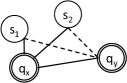
(a) For points.

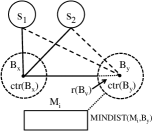
(b) For balls.

Figure 8: Outer-Triangle Distance Pruning.

Lemma 1

If $|S_{I}|\cdot d_{q_{x},q_{y}}-\sum\nolimits_{i=1}^{|S_{I}|}d_{s_{i},q_{x}}+(p-|S_{I}|)\cdot d_{v_{\min},q_{y}}\geq D$, $q_{y}$ never produces a better solution for any set of candidates expanded from $S_{I}$.

Proof 4

In the above inequality, the first two terms represent a lower bound on the total spatial distance from $S_{I}$ to $q_{y}$, and the third term is a lower bound on the total spatial distance from $q_{y}$ to any $(p-|S_{I}|)$ candidates in $S_{R}$. As shown in Figure 8(a), from triangular inequality, if $d_{q_{x},q_{y}}\geq\max_{s_{i}\in S_{I}}d_{s_{i},q_{x}}$, then $d_{q_{x},q_{y}}-d_{s_{i},q_{x}}<d_{s_{i},q_{y}}$, $\forall 1\leq i\leq|S_{I}|$ must hold. Therefore, $\sum\nolimits_{i=1}^{|S_{I}|}(d_{q_{x},q_{y}}-d_{s_{i},q_{x}})\leq\sum_{i=1}^{|S_{I}|}d_{s_{i},q_{y}}$, which can be written as $|S_{I}|\cdot d_{q_{x},q_{y}}-\sum\nolimits_{i=1}^{|S_{I}|}d_{s_{i},q_{x}}\leq\sum_{i=1}^{|S_{I}|}d_{s_{i},q_{y}}$. Note that $d_{q_{x},q_{y}}\geq\max_{s_{i}\in S_{I}}d_{s_{i},q_{x}}$ is necessary to be satisfied, otherwise the left-hand-side of $d_{q_{x},q_{y}}-d_{s_{i},q_{x}}<d_{s_{i},q_{y}}$ is not guaranteed to be a non-negative value, and $\sum\nolimits_{i=1}^{|S_{I}|}(d_{q_{x},q_{y}}-d_{s_{i},q_{x}})$ is not able to act as a lower bound on $\sum_{i=1}^{|S_{I}|}d_{s_{i},q_{y}}$. On the other hand, $(p-|S_{I}|)d_{v_{\min},q_{y}}$ is a lower bound on the total spatial from $(p-|S_{I}|)$ candidates in $S_{R}$ to activity location $q_{y}$. Therefore, $|S_{I}|\cdot d_{q_{x},q_{y}}-\sum\nolimits_{i=1}^{|S_{I}|}d_{s_{i},q_{x}}+(p-|S_{I}|)d_{v_{\min},q_{y}}$ is a lower bound on the total spatial distance from any set of $p$ candidates expanded from $S_{I}$ to $q_{y}$. In summary, if Outer-Triangle Distance Pruning condition holds, the total spatial distance from any set of $p$ candidates expanded from $S_{I}$ to $q_{y}$ always exceeds or equals to $D$.

Since $\sum\nolimits_{i=1}^{|S_{I}|}d_{s_{i},q_{x}}$ is computed when we access $q_{x}$, we only need to compute $d_{q_{x},q_{y}}$ instead of each $d_{s_{i},q_{y}}$. More importantly, it is possible to improve Outer-Triangle Distance Pruning from a single location to a ball of locations, as shown in Figure 8(b), to prune multiple redundant activity locations in the early stages of MAGS.

Specifically, when we consider two balls $B_{x}$ and $B_{y}$ instead of two locations $q_{x}$ and $q_{y}$, a lower bound on the spatial distance from $s_{i}\in S_{I}$ to any location in $B_{y}$ can be computed as $d_{ctr(B_{x}),ctr(B_{y})}-d_{s_{i},ctr(B_{x})}-r(B_{y})$, as shown in Figure 8(b). Therefore, a lower bound on the total spatial distance from $S_{I}$ to any location in $B_{y}$ is $|S_{I}|\cdot d_{ctr(B_{x}),ctr(B_{y})}-\sum\nolimits_{s_{i}\in S_{I}}d_{s_{i},ctr(B_{x})}-|S_{I}|\cdot r(B_{y})$. Moreover, MAGS also derives a lower bound of the remaining $p-|S_{I}|$ attendees as $(p-|S_{I}|)\min_{M_{i}\in U_{R}}MINDIST(M_{i},B_{y})$, where $\min_{M_{i}\in U_{R}}MINDIST(M_{i},B_{y})$ denotes a lower bound on the spatial distance from the locations in $B_{y}$ to its closest candidate attendees (i.e., $M_{i}$). In summary, given the currently best solution value $D$, ball $B_{x}$ and $S_{I}$, a ball $B_{y}$ can be pruned according to the following lemma.

Lemma 2

If $|S_{I}|\cdot d_{ctr(B_{x}),ctr(B_{y})}-\sum\nolimits_{s_{i}\in S_{I}}d_{s_{i},ctr(B_{x})}-|S_{I}|\cdot r(B_{y})+(p-|S_{I}|)\min_{M_{i}\in U_{R}}MINDIST(M_{i},B_{y})\geq D$, the activity locations within ball $B_{y}$ never produce a better solution for any set of $p$ candidates expanded from $S_{I}$.

Proof 5

As shown in Figure 8(b), if $\max_{s_{i}\in S_{I}}d_{s_{i},ctr(B_{x})}<d_{ctr(B_{x}),ctr(B_{y})}$, according to triangular inequality, $d_{ctr(B_{x}),ctr(B_{y})}-d_{s_{i},ctr(B_{x})}<d_{s_{i},ctr(B_{y})}$ must hold. Therefore, $\sum\nolimits_{s_{i}\in S_{I}}(d_{ctr(B_{x}),ctr(B_{y})}-d_{s_{i},ctr(B_{x})})=|S_{I}|\cdot d_{ctr(B_{x}),ctr(B_{y})}-\sum\nolimits_{s_{i}\in S_{I}}d_{s_{i},ctr(B_{x})}$ is a lower bound on $\sum\nolimits_{s_{i}\in S_{I}}d_{s_{i},ctr(B_{y})}$, i.e., the total distance from $S_{I}$ to $ctr(B_{y})$. In addition, since $d_{s_{i},ctr(B_{y})}-r(B_{y})$ is a lower bound on the distance from $s_{i}$ to any activity location in $B_{y}$, the lower bound on the total spatial distance from any activity location within $B_{y}$ to $S_{I}$ is thus $|S_{I}|\cdot d_{ctr(B_{x}),ctr(B_{y})}-\sum\nolimits_{s_{i}\in S_{I}}d_{s_{i},ctr(B_{x})}-|S_{I}|\cdot r(B_{y})$. Moreover, the lower bound on the total spatial distance from any activity location within $B_{y}$ to $(p-|S_{I}|)$ candidates in $S_{R}$ is $(p-|S_{I}|)\min_{M_{i}\in U_{R}}MINDIST(M_{i},B_{y})$. Therefore, if the condition of Outer-Triangle Distance Pruning holds, any activity location within $B_{y}$ never produces a better solution by incorporating any $(p-|S_{I}|)$ candidates into $S_{I}$, and $B_{y}$ thus can be safely pruned.

Compared with Lemma 1, Lemma 2 further aggregates the distance computation by including multiple balls in BallTree. Outer-Triangle Distance Pruning is performed each time $S_{I}$ is expanded. Note that $\sum\nolimits_{s_{i}\in S_{I}}d_{s_{i},ctr(B_{x})}$ is computed when accessing ball $B_{x}$. Therefore, Outer-Triangle Distance Pruning is able to prune multiple balls without recomputing $\sum\nolimits_{s_{i}\in S_{I}}d_{s_{i},ctr(B_{x})}$ each time.

Inner-Triangle Distance Pruning (ITDP). Outer-Triangle Distance Pruning derives the distance lower bounds based on the distance from $S_{I}$ to another previously-calculated activity location. On the other hand, the idea of Inner-Triangle Distance Pruning is that, when the attendees in $S_{I}$ are sparser, the total spatial distance from $S_{I}$ to some activity locations may also increase. Therefore, Inner-Triangle Distance Pruning removes redundant activity locations by deriving the lower bounds of the total spatial distance from attendees in $S_{I}$ to activity locations, based on the spatial distances of attendees in $S_{I}$.

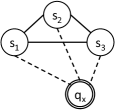
(a) For points.

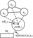
(b) For balls.

Figure 9: Inner-Triangle Distance Pruning.

Figure 9(a) shows a case where $S_{I}$ contains three attendees. In this case, the distance among each pair of attendees in $S_{I}$, i.e., $d_{s_{i},s_{j}}$ (solid lines) is used to derive a lower bound on the total spatial distance from $s_{i}$, $s_{j}$ to $q_{x}$ (dotted lines), i.e., $d_{s_{i},q_{x}}+d_{s_{j},q_{x}}>d_{s_{i},s_{j}}$. Therefore, Figure 9(a) shows a set of lower bounds on the spatial distance from $s_{i}$ to any location $q_{x}$: 1) $d_{s_{1},q_{x}}+d_{s_{2},q_{x}}>d_{s_{1},s_{2}}$, 2) $d_{s_{1},q_{x}}+d_{s_{3},q_{x}}>d_{s_{1},s_{3}}$, and 3) $d_{s_{2},q_{x}}+d_{s_{3},q_{x}}>d_{s_{2},s_{3}}$. Summing them up, we have a lower bound on the total spatial distance from $S_{I}$ to $q_{x}$, i.e., $(|S_{I}|-1)\cdot\sum_{i=1}^{|S_{I}|}d_{s_{i},q_{x}}>\sum_{i=1}^{|S_{I}|-1}\sum_{j=i+1}^{|S_{I}|}d_{s_{i},s_{j}}$. On the other hand, since MAGS needs to move other $p-|S_{I}|$ attendees to $S_{I}$, a lower bound on the total spatial distance from them to $q_{x}$ is $(|p-|S_{I}|)\cdot d_{v_{\min},q_{x}}$, where $d_{v_{\min},q_{x}}$ denotes the minimum spatial distance from $q_{x}$ to any candidates in $S_{R}$. Therefore, Inner-Triangle Distance Pruning is specified in the following lemma.

Lemma 3

If $\left(\frac{1}{|S_{I}|-1}\sum_{i=1}^{|S_{I}|-1}\sum_{j=i+1}^{|S_{I}|}d_{s_{i},s_{j}}\right)+(p-|S_{I}|)d_{v_{\min},q_{x}}\geq D$ holds, $q_{x}$ never produces a better solution for any set of $p$ candidates expanded from $S_{I}$.

Proof 6

The first term of the above inequality is a lower bound on the total spatial distance from $S_{I}$ to $q_{x}$, and the second term is a lower bound on the total spatial distance to $q_{x}$ from any $(p-|S_{I}|)$ candidates in $S_{R}$. From triangular inequality, we have $d_{s_{i},q_{x}}+d_{s_{j},q_{x}}>d_{s_{i},s_{j}}$, $\forall 1\leq i,j\leq|S_{I}|$ and $i\neq j$, such as $d_{s_{1},q_{x}}+d_{s_{2},q_{x}}>d_{s_{1},s_{2}}$ and $d_{s_{2},q_{x}}+d_{s_{1},q_{x}}>d_{s_{2},s_{1}}=d_{s_{1},s_{2}}$ as shown in Figure 9(a). Therefore, $(|S_{I}|-1)\sum_{i=1}^{|S_{I}|}d_{s_{i},q_{x}}+(|S_{I}|-1)\sum_{j=1}^{|S_{I}|}d_{s_{j},q_{x}}>2\cdot\sum_{i=1}^{|S_{I}|-1}\sum_{j=i+1}^{|S_{I}|}d_{s_{i},s_{j}}$, where $(|S_{I}|-1)\sum_{i=1}^{|S_{I}|}d_{s_{i},q_{x}}=(|S_{I}|-1)\sum_{j=1}^{|S_{I}|}d_{s_{j},q_{x}}$. Consequently, $(|S_{I}|-1)\sum_{i=1}^{|S_{I}|}d_{s_{i},q_{x}}>\sum_{i=1}^{|S_{I}|-1}\sum_{j=i+1}^{|S_{I}|}d_{s_{i},s_{j}}$, and we have $\sum_{i=1}^{|S_{I}|}d_{s_{i},q_{x}}>\frac{1}{|S_{I}|-1}\sum_{i=1}^{|S_{I}|-1}\sum_{j=i+1}^{|S_{I}|}d_{s_{i},s_{j}}$. In other words, $\frac{1}{|S_{I}|-1}\sum_{i=1}^{|S_{I}|-1}\sum_{j=i+1}^{|S_{I}|}d_{s_{i},s_{j}}$ acts as a lower bound on the total spatial distance from $q_{x}$ to $S_{I}$. On the other hand, $(p-|S_{I}|)d_{v_{\min},q_{x}}$ is a lower bound on the total spatial to $q_{x}$ from any $(p-|S_{I}|)$ candidates in $S_{R}$. Therefore, $\left(\frac{1}{|S_{I}|-1}\sum_{i=1}^{|S_{I}|-1}\sum_{j=i+1}^{|S_{I}|}d_{s_{i},s_{j}}\right)+(p-|S_{I}|)d_{v_{\min},q_{x}}$ is a lower bound on the total spatial distance from any set of $p$ candidates expanded from $S_{I}$ to the activity location $q_{x}$. Therefore, if the condition of Inner-Triangle Distance Pruning holds, the total spatial distance from any set of $p$ candidates expanded from $S_{I}$ to $q_{x}$ must equal to or exceed $D$.

Note that $|S_{I}|-1$ must be included in the denominator to prevent overestimation of duplicated distance $d_{s_{i},s_{j}}$. In addition, the first term can be constructed incrementally as $S_{I}$ expands, which does not require recomputation at each iteration. Therefore, Inner-Triangle Distance Pruning can be performed efficiently.

It is more efficient to trim off multiple unnecessary activity locations all together. Since $\left(\frac{1}{|S_{I}|-1}\sum_{i=1}^{|S_{I}|-1}\sum_{j=i+1}^{|S_{I}|}d_{s_{i},s_{j}}\right)$ is a lower bound on the total spatial distance from $S_{I}$ to a point (the center of ball $B_{x}$ of locations), we can subtract this term with $|S_{I}|\cdot r(B_{x})$ to obtain a lower bound on the total spatial distance from $S_{I}$ to any location in $B_{x}$, as shown in Figure 9(b). Moreover, similar to OTDP, we can replace $(p-|S_{I}|)d_{v_{\min},q_{x}}$ in Lemma 3 by its lower bound $(p-|S_{I}|)\min_{M_{i}\in U_{R}}MINDIST(M_{i},B_{x})$. Therefore, given a ball $B_{x}$, all activity locations within $B_{x}$ can be safely pruned according to the following lemma.

Lemma 4

If $\left(\frac{1}{|S_{I}|-1}\sum_{i=1}^{|S_{I}|-1}\sum_{j=i+1}^{|S_{I}|}d_{s_{i},s_{j}}\right)-|S_{I}|\cdot r(B_{x})+(p-|S_{I}|)\min_{M_{i}\in U_{R}}MINDIST(M_{i},B_{x})\geq D$ holds, any activity location within ball $B_{x}$ never produces a better solution expanded from $S_{I}$.

Proof 7

As illustrated in Figure 9(b) and pointed out in Lemma 3, $\left(\frac{1}{|S_{I}|-1}\sum_{i=1}^{|S_{I}|-1}\sum_{j=i+1}^{|S_{I}|}d_{s_{i},s_{j}}\right)$ is a lower bound on the total spatial distance from $S_{I}$ to $ctr(B_{x})$. $|S_{I}|\cdot r(B_{x})$ is necessary to be incorporated to ensure that, $\left(\frac{1}{|S_{I}|-1}\sum_{i=1}^{|S_{I}|-1}\sum_{j=i+1}^{|S_{I}|}d_{s_{i},s_{j}}\right)-|S_{I}|\cdot r(B_{x})$ is a lower bound on the total spatial distance from $S_{I}$ to any activity location within $B_{x}$. On the other hand, $(p-|S_{I}|)\min_{M_{i}\in U_{R}}MINDIST(M_{i},B_{x})$ represents a lower bound on the total spatial distance from $(p-|S_{I}|)$ candidates in $S_{R}$ to $B_{x}$. Therefore, when the above condition holds, any activity location within $B_{x}$ never produces a better solution with any group of $p$ candidates expanded from $S_{I}$. Thus, $B_{x}$ can be safely pruned.

Activity Location Distance Pruning. Activity Location Distance Pruning exploits the MBRs in R-Tree and the balls in BallTree, to quickly filter out unqualified activity locations.

solution value $D$ and ball $B_{x}$, Activity Location Distance Pruning jointly considers a lower bound from the attendees in $S_{I}$ to $B_{x}$ and a lower bound from $(p-|S_{I}|)$ remaining candidates in $S_{R}$ to $B_{x}$. If the sum of the two lower bounds exceeds $D$, it concludes that $S_{I}$ and all activity locations within $B_{x}$ never produce a better solution with the total spatial distance smaller than $D$. Specifically, Activity Location Distance Pruning is based on Lemma 5 below.

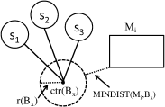
Figure 10: Activity Location Distance Pruning.

Lemma 5

If $\sum\nolimits_{s_{i}\in S_{I}}MINDIST(s_{i},B_{x})+(p-|S_{I}|)\min_{M_{i}\in U_{R}}MINDIST(M_{i},B_{x})\geq D$ holds, the activity locations within ball $B_{x}$ do not produce a better solution than the current solution corresponding to $D$.

Proof 8

As shown in Figure 10. $MINDIST(s_{i},B_{x})=d_{s_{i},B_{x}}-r(B_{x})$ is a lower bound on the distance from $s_{i}$ to any activity location within $B_{x}$. Thus, $\sum\nolimits_{s_{i}\in S_{I}}MINDIST(s_{i},B_{x})$ represents a lower bound on the total spatial distance from $S_{I}$ and any activity locations within Ball $B_{x}$, and $(p-|S_{I}|)\min_{M_{i}\in U_{R}}MINDIST(M_{i},B_{x})$ represents a lower bound on the total spatial distance from $(p-|S_{I}|)$ remaining candidates to any activity locations in $B_{x}$. Therefore, when the above condition holds, any activity location within $B_{x}$ never produces a better solution when any $(p-|S_{I}|)$ candidates are selected into $S_{I}$. Therefore, $B_{x}$ can be safely pruned.

Although the above strategy is simple, it still incurs high computation overhead because $|S_{I}|$ distance computations performed for each ball $B_{x}$ to find the lower bound. In other words, the above strategy incurs $|S_{I}|\cdot n$ distance computations, where $n$ is the number of balls. In the following, therefore, we propose two strategies which utilize the information of activity locations and the relationship of attendees in $S_{I}$ to reduce the number of distance computations.

Here we briefly analyze the above distance pruning strategies. Let $m$ denote the number of distance computations for $(p-|S_{I}|)\cdot\min_{M_{i}\in U_{R}}MINDIST(M_{i},B_{x})$. Activity Location Distance Pruning incurs the highest computation overhead, i.e., $(n\cdot|S_{I}|+m)$, as distance computations are required for $n$ balls (for each ball, it derives $MINDIST(s_{i},B_{x}),\forall s_{i}\in S_{I}$). On the other hand, Outer-Triangle Distance Pruning incurs $(|S_{I}|+n+m-1)$ distance computations, for $n$ balls in the worst case, including $|S_{I}|$ computations for the total spatial distance from $S_{I}$ to $ctr(B_{x})$, and $(n-1)$ computations for the distances from $ctr(B_{x})$ to the centers of the other $(n-1)$ balls. Similarly, when deriving the lower bound on $S_{I}$ and $B_{x}$, Inner-Triangle Distance Pruning only considers the distances between each pair of attendees in $S_{I}$, which can be computed incrementally and cached in early stages. Therefore, each time a new attendee is added to $S_{I}$, Inner-Triangle Distance Pruning performs $(|S_{I}|-1+m)$ distance computations for $n$ balls. Therefore, Outer-Triangle Distance Pruning and Inner-Triangle Distance Pruning are much more efficient than Activity Location Distance Pruning.

5.6 Discussions

User interests and existence of sponsors. We propose a generalized model to support the scenarios in terms of user interests. Let $\eta_{v,q}$ denote the interest measure (i.e., how an individual $v$ prefers a candidate location $q$) of a person $v$ in an activity to be held at location $q$. A small interest measure $\eta_{v,q}$ implies that $v$ highly prefers the activities to be associated with $q$. Similar to the spatial radius constraint in SSGQ and MRGQ, a new interest constraint $\eta_{v,q}<h$ is added to the two problems, where $h$ denotes the interest threshold of an activity. For a candidate member $v$ that prefers only karaoke studios and bars, the interest measure from $v$ to coffee shops will be set to a large value exceeding the threshold. Thus, $v$ in this case will never be selected for an activity in $q$.

MRGQ and SSGQ can also flexibly handle the case when sponsors of the activity exist. Here, we describe a generalized graph model for the scenarios with sponsors. The sponsors are represented by a set $S$ of new nodes in SSGQ and MRGQ. Here each sponsor $s$ in $S$ is connected to a person $v$ if $s$ is correlated to $v$, e.g., $v$ is an employee, a former student, or a regular customer of $s$. This link information can be acquired from the address directories, personal Facebook profiles, or customer databases. To support SSGQ and MRGQ with sponsors, the set $S$ is added to the solution at the beginning of SSGS and MAGS. As such, these two algorithms will automatically find a solution group with correlation to $S$ (i.e., the attendees that $S$ would like to sponsor). Moreover, if the activity locations are provided by a sponsor, such as a chain restaurant, all branches of the chain restaurant group can be included in the candidate location set $Q$. Note that the group size $p$ needs to be increased by $\left|S\right|$ in the scenarios with sponsors, and the representatives of each sponsor can also be initially added to the solution group.

Dynamically changing user locations. To index user locations, one approach is to employ the fundamental R-Tree. If user locations are changed frequently, however, this approach is likely to incur frequent index updates or otherwise record outdated and inaccurate information. A more promising approach is to exploit R-Tree extensions that are specifically designed for dynamic environments, such as Time-Parameterized R-Tree (TPR-Tree) [22] or an improved version of TPR-Tree, TPR*-Tree [23]. Similar to conventional R-Trees, TPR-Tree adopts Minimum Bounding Rectangles (MBR) to hierarchically index the spatial objects (i.e., the locations of the users). However, instead of recording objects’ locations at individual timestamps, TPR-Tree incorporates the velocity of each object to predict their upcoming positions, and thus updates are only triggered when the velocity changes. This strategy significantly reduces the number of updates. In other words, the MBR of an object or a tree node is a function of time.

More specifically, each dynamically changing location of a user in the TPR-Tree is represented as 1) an MBR that denotes its extent at some reference time (a system parameter), and 2) its current velocity vector. The velocity vector of an MBR is represented by the largest velocity of an object within the MBR in each direction. This strategy ensures that the MBR always encloses the underlying objects in the future. With the above information, the future MBRs and the objects’ locations are not stored explicitly, but are quickly computed based on the locations at the reference time and the velocity vectors. Figure 11 presents an example of the MBR and velocity vectors of three objects, i.e., $a$, $b$, and $c$. The velocity vector of each object is shown as solid arrows, and the velocity vector of the MBR is represented by dashed arrows. Figure 11(a) presents the locations of the objects and the enclosing MBR at reference time $0$. In the next time slot shown in Figure 11(b), the locations of the objects are changed, and the enclosing MBR is enlarged to enclose all objects. As shown in this example, TPR-Tree only stores the locations of the objects and the corresponding MBR at the reference time, and the locations of the objects with the enclosing MBR in the future can then be computed with the velocity vectors.

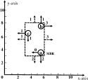
(a) Boundaries at reference time $0$.

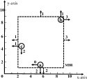
(b) Boundaries at time $1$.

Figure 11: An example of the MBR and objects with velocity vectors.

To support dynamic environments in this paper, we replace R-Tree with TPR-Tree. Similar to the TPR-Tree problem, a parameter $t_{f}\geq 0$ is included in SSGQ and MRGQ to ensure that the optimal group is returned for dynamic environments from now to $t_{f}$ time units afterward. The ordering and pruning strategies of SSGS and MAGS are performed in the same way, except that the extents of the MBRs and the user locations have to be calculated before SSGS and MAGS. On the other hand, the BallTree in this paper only indexes the activity locations (e.g., restaurants, theaters, etc.) and thus does not need to be updated frequently.

6 Tractability of MRGQ in Threshold Graph

In Graph Theory, analyzing the tractability of NP-Hard graph problems in special graph classes is very important for theoreticians, e.g., [16][17]. Therefore, in addition to the inapproximibility of MRGQ analyzed above, we also prove that MAGS can find the optimal solution in polynomial time in a special graph class, namely threshold graph, which is defined as follows [15].

Definition 1

Given a threshold $\tau$ and a graph $G=(V,E)$ with a non-negative weight $w_{v}$ for each vertex $v\in V$, $G$ is called a threshold graph if $w(U)=\sum_{v\in U}w_{v}\leq\tau$ holds for every subset $U\subseteq V$ with every two nodes in $U$ sharing no edge between them.

Let $deg_{G}(v)$ denote the degree of $v\in V$. A degree partition $D(V)$ of $V$ divides $V$ into $m+1$ non-overlapping subsets $D_{0},D_{1},..,D_{m}$, i.e., $\bigcup_{\forall i}D_{i}=V$. Each subset $D_{i}$ includes all the vertices with degree $\delta_{i}$, and $\delta_{i}>\delta_{j}$ if $i>j$. When $\tau=m$ and $w_{v}=deg_{G}(v)$, we exploit the following theorem in the literature [15] to prove that MAGS can obtain the optimal solution in polynomial time in a threshold graph.

Theorem 4

[15] Let $\widehat{G}=(\widehat{V},\widehat{E})$ be a threshold graph with degree partition $D(\widehat{V})$. For every pair of vertices $u\in D_{i}$ and $v\in D_{j}$, $u$ is connected to $v$ in $\widehat{G}$ if and only if $i+j>m$. Therefore, every vertex in $D_{i}$ shares the same neighbors.

We first describe the tie-breaking strategy for Socio-Spatial Ordering in MAGS. Specifically, for any set $\widetilde{V}\subseteq S_{R}$ of vertices with the same spatial distance to each query point $q_{i}$, the tie-breaking strategy checks if the vertices in $\widetilde{V}$ satisfy Eq. (1) in descending order of their vertex degrees. Therefore, the vertex $v\in\widetilde{V}$ with the maximum $deg_{G}(v)$ is first examined by Eq. (1) and moved into $S_{I}$ if $v$ satisfies Eq. (1). Moreover, we employ a pre-processing strategy to remove unqualified vertices from the input graph $\widehat{G}$, which works both when $\widehat{G}$ is a general graph or $\widehat{G}$ is a threshold graph. Given the social network $\widehat{G}$ with parameters $k$ and $p$, the pre-processing strategy iteratively removes from $\widehat{G}$ every vertex $v$ with fewer than $p-k-1$ neighbors, along with $v$’s incident edges. The iteration repeats until no more vertices can be removed and produces a graph $G$. Any removed vertex $v$ cannot form a feasible graph with other vertices in $\widehat{G}$, because even when all the neighbors of $v$ (i.e., $N_{v}$) are included in the same group $F$, there is still at least one vertex in $N_{v}\cup\{v\}$ with fewer than $p-k-1$ neighbors in $F$. The above process is called core decomposition, and the remaining graph $G$ is a maximal $(p-k-1)$-core [18], where $G\subseteq\widehat{G}$ is the largest graph such that each vertex has at least $p-k-1$ neighbors in $G$. The pre-processing strategy can be done in $O(|\widehat{E}|)$ time [19]. Intuitively, if $|G|<p$, then there exists no solution to MRGQ.

Note that $D_{j}$ is the degree partition on $\widehat{G}$, instead of $G$ after the core decomposition. Let $V(G)$ denote the set of vertices in $G$, and let $\widehat{j}$ denote the minimum $j$ such that $D_{j}\cap V(G)\neq\varnothing$. In other words, $D_{0},D_{1},..,D_{\widehat{j}-1}$ are all removed during core decomposition. The following theorem first compares $\widehat{G}$ and $G$.

Theorem 5

For input threshold graph $\widehat{G}$ and the graph $G$ after core decomposition, $\bigcup_{i=\widehat{j}}^{m}D_{i}=V(G)$ holds, and the neighbors of every vertex in $D_{i}$ are also the neighbors of every vertex in $D_{j}$ if $i<j$.

Proof 9

Apparently, $\bigcup_{i=\widehat{j}}^{m}D_{i}\supseteq V(G)$ since $G\subseteq\widehat{G}$, and thus we prove that $\bigcup_{i=\widehat{j}}^{m}D_{i}\subseteq V(G)$ by contradiction. Assume $u\in D_{r}$ for some $r\geq\widehat{j}$, but $u\notin V(G)$. Given a vertex $x$ in $D_{\widehat{j}}\cap V(G)$ and any vertex $y\in V(G)$ sharing an edge with $x$, if $y\in D_{s},$ $\widehat{j}\leq s\leq m$, according to Theorem 4, $\widehat{j}+s>m$ must hold; otherwise, $x$ and $y$ would not share an edge. Since $\widehat{j}$ is the minimum number such that $D_{\widehat{j}}\cap V(G)\neq\varnothing$, $r+s>m$ must hold, implying that $u$ has an edge with $y$ because $r\geq\widehat{j}$. From the definition of threshold graph, $u$ also share edges with all neighbors of $x$. Therefore, the number of $u$’s neighbors in $V(G)$ is no smaller than $x$ does, and $u$ should not be removed by the pre-processing strategy because $x\in D_{\widehat{j}}\cap V(G)$. Therefore, this contradiction proves that $\bigcup_{i=\widehat{j}}^{m}D_{i}=V(G)$ holds. Moreover, since vertex $u$ in $D_{i}$ is connected to $w$ in $D_{n}$ if and only if $i+n>m$ according to Theorem 4, vertex $v$ in $D_{j}$ is also connected to $w$ in $D_{n}$ if $j>i$ because $j+n>i+n>m$. Therefore, the neighbors of every vertex in $D_{i}$ are also the neighbors of every vertex in $D_{j}$ if $i<j$.

In other words, core decomposition only trims the vertices with smaller degrees, and if any vertex in $D_{i}$ is removed, the above theorem manifests that all the other vertices in $D_{i}$ will be pruned as well. According to Theorem 4, every vertex in $D_{i}$ still shares the same neighbors. In the following, we provide the theoretical result for MAGS in Theorem 6. In Graph Theory, since each vertex $v$ of a threshold graph is not associated with a spatial distance to $q_{i}\in Q$, we first assume that $d_{v,q_{i}}=1$ for $\forall v\in V,q_{i}\in Q$.

Theorem 6

Let $\widehat{G}=(\widehat{V},\widehat{E})$ be a threshold graph with degree partition $\widehat{V}=D_{0}\cup D_{1}\cup\cdots\cup D_{m}$ and $\beta=\max\{i:|D_{i}|+\cdots+|D_{m}|\geq p\}$. Given an $MRGQ(p,Q,k,t)$ for $\widehat{G}$, MAGS stops (either returning the optimal solution or returning no solution) in polynomial time if $d_{v,q_{i}}=1,\forall v\in\widehat{V},q_{i}\in Q$.

Proof 10

We employ All-Pair Distance Ordering for MAGS here. If after core decomposition, the resulting graph has fewer than $p$ vertices, i.e., $|G|<p$, there is no feasible solution, and MAGS stops in $O(|\widehat{E}|)$ time (i.e., only the core decomposition is performed). Otherwise, if $|G|\geq p$, we prove that there exists at least one feasible solution, and we prove the theorem by examining two different cases for $\beta$: $\beta>\lfloor\frac{m}{2}\rfloor$ and $\beta\leq\lfloor\frac{m}{2}\rfloor$.

(1) $\beta>\lfloor\frac{m}{2}\rfloor$. We prove that MAGS can find the optimal solution by generating only $p$ nodes in the branch-and-bound tree. From Theorem 4 and Theorem 5, every two vertices $u$ and $v$ in $\bigcup_{i=\lfloor\frac{m}{2}\rfloor+1}^{m}D_{i}$ are connected by an edge in $G$. Since $|D_{\beta}|+..+|D_{m}|\geq p$, the first $p$ vertices selected and examined by Socio-Spatial Ordering and the tie-breaking strategy must belong to $\bigcup_{i=\lfloor\frac{m}{2}\rfloor+1}^{m}D_{i}$ and form a path of length $p$ from the root in the branch-and-bound tree. Since every two vertices $u,v\in\bigcup_{i=\lfloor\frac{m}{2}\rfloor+1}^{m}D_{i}$ are connected according to Theorem 4, $F$ is a feasible group. In the $p$-th node generated in the branch-and-bound tree, $\langle F,q_{ref}\rangle$ is a feasible solution in $G$, where $q_{ref}$ can be derived by All-Pair Distance Ordering. Because $d_{v,q_{i}}=1$ here, $\forall v\in V,q_{i}\in Q$, $\langle F,q_{ref}\rangle$ is the optimal solution, i.e., $q^{\ast}=q_{ref}$. Afterwards, the distance pruning strategies of MAGS are performed exactly $p$ times (one time for each branch-and-bound node except the leaf node, and one time for the root of the branch-and-bound tree) to conclude that no further search is required. Since $\langle F,q^{\ast}\rangle$ is the optimal solution in $G$, it will also be the optimal solution in $\widehat{G}$ due to $d_{v,q_{i}}=1,\forall v\in\widehat{V},q_{i}\in Q$.

(2) $\beta\leq\lfloor\frac{m}{2}\rfloor$. In this case, we prove that MAGS can also find the optimal solution by generating exactly $p$ nodes in the branch-and-bound tree. In MAGS, Socio-Spatial Ordering and the tie-breaking strategy first move the vertices in $\bigcup_{i=\beta+1}^{m}D_{i}$ into $S_{I}$ (vertices in $D_{i}$ are moved into $S_{I}$ earlier than those in $D_{j}$ if $i>j$), and then move the rest $p-|S_{I}|$ vertices from $D_{\beta}$ to $S_{I}$ to construct the group $F$. Moving these $p$ vertices into $S_{I}$ creates the first $p$ nodes in the branch-and-bound tree and builds up a path of length $p$ from the root.

In the following, we prove that $F$ is a feasible group in $G$. We first examine the vertices in $F$ that are drawn from $\bigcup_{i=\beta}^{\lfloor\frac{m}{2}\rfloor}D_{i}$. Let $v\in F$ and $v\in\bigcup_{i=\beta}^{\lfloor\frac{m}{2}\rfloor}D_{i}$. According to Theorem 4 and Theorem 5, all neighbors of $v$ in $G$ must belong to $\bigcup_{i=\lfloor\frac{m}{2}\rfloor+1}^{m}D_{i}$. Since $G$ is a $(p-k-1)$-core, and the extracted subgraph $F$ contains all the vertices in $\bigcup_{i=\lfloor\frac{m}{2}\rfloor+1}^{m}D_{i}$, $v$ must have at least $p-k-1$ neighbors in $F$. By contrast, for every vertex $u\in F$ drawn from $\bigcup_{i=\lfloor\frac{m}{2}\rfloor+1}^{m}D_{i}$, since the neighbors of every vertex in $D_{i}$ with $i\leq\lfloor\frac{m}{2}\rfloor$ are also the neighbors of every vertex in $D_{j}$ with $j>\lfloor\frac{m}{2}\rfloor$ according to Theorem 5, $u$ must have no fewer neighbors than that of $v$ in $F$, where $v\in F$ is any vertex drawn from $\bigcup_{i=\beta}^{\lfloor\frac{m}{2}\rfloor}D_{i}$. From the above description, a vertex $v\in F$ drawn from either $\bigcup_{i=\beta}^{\lfloor\frac{m}{2}\rfloor}D_{i}$ or $\bigcup_{i=\lfloor\frac{m}{2}\rfloor+1}^{m}D_{i}$ must have at least $(p-k-1)$ neighbors in $F$. Therefore, $F$ is a feasible group. Similar to case (1), $\langle F,q_{ref}\rangle$ is the optimal solution, where $q_{ref}$ is obtained from All-Pair Distance Ordering. Then, the distance pruning strategies conclude that no further search is needed, and MAGS stops.

Time Complexity. In the following, we analyze the detailed time complexity of constructing these $p$ nodes. The pre-processing strategy takes $O(|\widehat{E}|)$ time. Before each of the $p$ nodes in the branch-and-bound tree is constructed, MAGS extracts $v_{c}\in S_{R}$ and $q_{ref}\in Q_{I}$ from the lists $U_{R}$ and $U_{B}$. During the examinations of $U_{R}$ and $U_{B}$, when the MBR $M_{i}\in U_{R}$ and ball $B_{j}\in U_{B}$ satisfying the score function in Eq. (7) are identified, each of the three distance pruning strategies in Sec. 5.5 is performed once. In the worst case, each time when APDO obtains $v_{c}$ and $q_{ref}$, each internal node of R-Tree and BallTree is accessed. Therefore, $\max\{|V|,|Q|\}$ times of extracting $M_{i}$ and $B_{j}$ satisfying Eq. (7) are performed, and $\max\{|V|,|Q|\}$ times of each distance pruning strategy is also performed. Since extracting $M_{i}$ and $B_{j}$ satisfying Eq. (7) takes $O(|S_{I}||V||Q|)=O(p|V||Q|)$ time, and OTDP, ITDP and ALDP each takes $O(|Q|)$ time, the time complexity for MAGS to extract each pair of $v_{c}\in S_{R}$ and $q_{ref}\in Q_{I}$ is thus $O(\max\{|V|,|Q|\}(p|V||Q|))$. Therefore, for the $p$ nodes in the branch-and-bound tree, it takes $O(p^{2}\max\{|V|,|Q|\}(|V||Q|))$ time for extracting $v_{c}$ and $q_{ref}$ and performing the distance pruning strategies.

On the other hand, for the $p$ nodes in the branch-and-bound tree, $p$ times of Eq. (1) checking and tie-breaking strategy are performed, which takes $O(p^{3}+p|V|\log|V|)$. Also, $p$ times of Familiarity Pruning (Eqs. (4), (5)) are performed, which takes $O(p|V|^{2})$. Moreover, $p$ additional times of $v_{c}$ and $q_{ref}$ extractions (with distance pruning strategies) are performed to conclude that no further search is needed, which takes $O(p^{2}\max\{|V|,|Q|\}(|V||Q|))$ time. Therefore, the overall time complexity of MAGS is $O(|\widehat{E}|)+O(p^{3}+p|V|\log|V|)+O(p|V|^{2})+2\cdot O(p^{2}\max\{|V|,|Q|\}(|V||Q|))$. Since $|V|=O(|\widehat{V}|)$, where $\widehat{G}=(\widehat{V},\widehat{E})$ is the input graph before pre-processing. Therefore, the time complexity is $O(|\widehat{E}|+p^{2}\max\{|\widehat{V}|,|Q|\}(|\widehat{V}||Q|))$.

7 Experimental Results

We implement SSGQ in Facebook and recruit 206 people from various backgrounds (e.g., students, and public and private sector workers) to compare solution quality and time overhead for answering SSGQ and MRGQ via manual coordination and our proposed algorithms. Each user completes 24 SSGQ tasks and 20 MRGQ tasks with the social graphs extracted from their social networks in Facebook, together with their spatial locations sampled from their Facebook Checkin records.

In addition to the real dataset collected from the 206 study participants, we evaluate the performance and the solution quality of SSGS, SSGMerge (the heuristic algorithm for SSGQ mentioned in Section 4) and MAGS using a large real dataset, DataSet_4SQ, obtained by crawling Foursquare [20], one of the most representative LBSNs, for a month. DataSet_4SQ contains both the social and spatial information of 153,577 individuals. Moreover, we also compare MAGS with two relevant algorithms, namely Geo-Social Circle of Friend Query (gCoFQ) [13] and p-Nearest Neighbor (pNN), to evaluate the solution quality and performance. In addition to DataSet_4SQ, we also evaluate MAGS for MRGQ on a large real dataset, DataSet_Youtube [21], which is a social network extracted from Youtube video-sharing website with 1,134,890 individuals. The activity location $q$ for SSGQ and $Q$ for MRGQ are randomly selected from DataSet_4SQ, and we measure 50 samples in each scenario.

7.1 User Study

We perform the user study with 24 and 20 tasks for SSGQ and MRGQ, respectively. The 24 tasks in the user study of SSGQ span various $p$ and network sizes, where the spatial radius, $t$ is fixed to 10 km. Different $k$ are assigned in the first 12 tasks, while $k$ is not specified in the other 12 tasks, to let each user freely select $p$ people for finding out the familiarity preferred by each person in activities with different $p$.

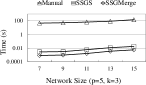
(a) Coordination time.

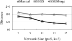
(b) Solution quality.

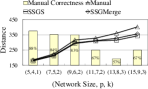
(c) Solutions with given $k$.

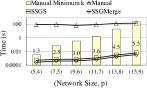
(d) Time without given $k$.

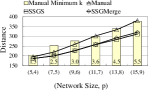
(e) Solutions without given $k$.

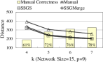
(f) Solutions with different $k$.

Figure 12: Results of user study.

Figures 12(a)-(f) compare manual coordination, SSGS and SSGMerge to answer SSGQ in the user study. Figure 12(a) presents the time to find the solutions in different scenarios. The result indicates that SSGQ is challenging for manual coordination, especially for a large network size. In contrast, SSGS obtains the optimal solution with less than 0.01 second, while SSGMerge obtains a near-optimal solution with much less time. Figure 12(b) with $p=5$ and $k=3$ demonstrates that the solutions from manual coordination require larger spatial distance and thereby are not optimal. With a larger network size, i.e., more friends nearby, it is easier to find a group of attendees with a smaller total spatial distance to $q$. In addition, the solution quality in Figure 12(c) shows that even in $p=5$, the solutions obtained by manual coordination is not guaranteed to follow the familiarity constraint, according to the correctness rate shown in Figure 12(c), because it is very challenging for a person to jointly minimize the total spatial distance and ensure the familiarity constraint. Moreover, the correctness rate drops dramatically as the network size increases. On the other hand, as shown in Figure 12(b) and 12(c), SSGMerge obtains solutions which are very close to the optimal solution, this is because SSGMerge effectively utilizes the intermediate solutions to construct good solutions.

In Figures 12(d) and 12(e), we let each user freely select $p$ people to find out the familiarity preferred by each person in activities with different $p$. The minimum $k$ here represents the smallest $k$ for each manual solution to follow the familiarity constraint. With this parameter extracted from the manual solution, we regard it as an input parameter for an SSGQ in the same social network. The results demonstrate that SSGS and SSGMerge can find better solutions following the same $k$ with a smaller time. In other words, even when a user does not specify $k$, it is possible to analyze the previous manual coordination results and find out a suitable $k$ for the user, such that SSGS and SSGMerge are able to find solutions in each query afterward.

Figure 12(f) with the network size as 15 and $p$ as 9 compares the results of different $k$. As $k$ decreases, the correctness rate of manual coordination drops because it becomes more difficult for a user to find a tighter social group with the same number of attendees. Moreover, the solution obtained by manual coordination is still worse than the solution of SSGS and SSGMerge even with a loose requirement on social connectivity, i.e., a large $k$.

These MRGQ tasks span various $p$, $k$, and $|Q|$, where $t$ is fixed to 10 km. In the user study, MAGS is equipped with APDO and all the proposed pruning strategies. We also compare the solution quality with an algorithm called GreedyManual (GM), which imitates the behavior of manual coordination. GM first finds the candidates within radius $t$ of each activity location and picks the activity location which has the largest number of candidates nearby. Afterwards, if there exists a feasible group, GM returns it. Otherwise, it repeats the above procedure with the remaining activity locations.

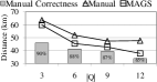
(a) Solution quality.

(b) Solutions with given $k$.

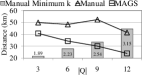
(c) Solutions without given $k$.

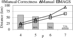
(d) Solutions with given $p$.

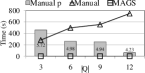
(e) Time without given $p$.

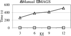
(f) Time of activity organization.

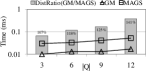
(g) Comparisons of GM.

(h) User satisfaction.

Figure 13: Results of user study.

Figures 13 compares manual coordination and MAGS to answer MRGQ in the user study. Figure 13(a) demonstrates that the solutions from manual coordination incur larger spatial distance and thereby are not optimal. When the number of activity locations increases, it is easier to find a group of attendees and an activity location with a smaller total spatial distance. In addition, the correctness rate in Figure 13(b) shows that even when $p=5$, the solutions obtained by manual coordination are not guaranteed to follow the social constraint, especially for a smaller $k$, because it is very challenging for a user to jointly minimize the total spatial distance and ensure the social constraint. In Figure 13(c), we let each user freely select $5$ people and analyze the familiarity parameter preferred by each person in activities. The minimum $k$ here represents the smallest $k$ to meet the familiarity constraint in user selection. With this parameter extracted from the manual solution, we regard it as an input parameter for an MRGQ query in the same social network. The results demonstrate that users are difficult to handle small $k$ and large $|Q|$ due to the need to examine many more combinations. Thus, the distances obtained by manual coordination are more deviated from the optimal solution obtained by MAGS.

Figures 13(d) shows that as $p$ increases, the correctness rate and solution quality of manual coordination significantly deteriorate because it becomes more difficult for a user to find a tight social group. In Figure 13(e), each user can freely select any number of people for forming the group with $k=3$. Manual p in this figure indicates the average group size measured in the user study. As $|Q|$ increases, the selected group size drops because it becomes more challenging to find the optimal group. Moreover, users need much more time to find the group when $|Q|$ grows, even with a small group size and a loose requirement on the social connectivity, i.e., $p=\{4,5\}$ and $k=3$. Finally, Figure 13(f) presents the time spent to find the solutions in different scenarios. The result indicates that MRGQ is challenging for manual coordination, especially for a large number of potential candidate locations.

Figure 13(g) compares the computation time and solution quality of GreedyManual (GM) and MAGS. Although GM obtains the solutions within a smaller time, the solution quality is much worse than MAGS. This is because GM stops when a feasible group is obtained, which cannot effectively obtain the optimal solution.

Since MRGQ can also consider the user interests (discussed in Section 5.6), we also compare the user satisfaction with or without considering user interests. We ask the users to choose 20 activity locations in MRGQ, where each location is tagged as coffee shop, restaurant, bar, etc. The interest measure of each activity location $q_{i}$ to each user $u$ is specified as $\eta_{u,q_{i}}$ between 0 and 1 by the user. We let each user compare the groups selected by MAGS and the user herself. Figure 13(h) with $p=7$ and $k=3$ compares the user satisfaction with and without user interests incorporated. The results manifest that $68\%$ and $75\%$ of the users agree that the groups selected by MAGS outperform the manually selected groups before and after incorporating the interests, respectively. Moreover, the increment of the users that choose ”Better” after incorporating the user interests mainly come from those who previously chose ”Acceptable”. The results demonstrate that incorporating user interests indeed improves the user satisfaction.

7.2 Performance Evaluation of Proposed Algorithms for MRGQ

We evaluate the effectiveness and efficiency of the proposed algorithms for MRGQ. APDO and SRDO denote MAGS with All-Pair Distance Ordering and Single-Reference Distance Ordering (a simplified version of APDO, which is mentioned in Section 5.4), respectively, while Socio-Spatial Ordering and Familiarity Pruning mentioned in Section 5.1 are also included. In our experiments, unless specifically indicated, we set $k=4$, $p=8$, $|Q|=10,000$, and the maximum value of $t$ is 15 km.

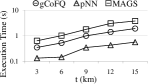
(a) Computation time.

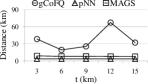
(b) Solution quality.

(c) Familiarity constraint.

(d) Social diameter.

Figure 14: Comparisons with relevant works on DataSet_4SQ.

Figure 14 first compares MAGS in MRGQ with the related works on DataSet_4SQ, where MAGS is equipped with APDO, Socio-Spatial Ordering and the proposed pruning strategies. 1) Geo-Social Circle of Friend Query (gCoFQ) [13] aims to find a group of $p$ people to minimize the linear combination of the social diameter and spatial diameter (maximum spatial distance between each pair of group members) of the selected group. In other words, there is no activity location in gCoFQ. In the experiments, gCoFQ is implemented to limit the spatial diameter within $2t$, and the nearest activity location after gCoFQ identifies the group is returned as the solution. On the other hand, 2) pNN extracts the group of $p$ members along with their nearest activity location without considering the familiarity constraint. Figures 14(a) and 14(b) compare the computation time and solution quality. Although pNN obtains the group with the minimum time and distance, as shown in Figure 14(c), the minimum $k$ of the obtained group (i.e., the minimum number of unfamiliar members each attendee has in the group) is far from the specified $k$ value, i.e., $k=4$. In other words, the solution returned by pNN is not feasible to MGRQ. The solution quality of gCoFQ is worse than the other two algorithms because gCoFQ does not examine activity locations during the group formation process, while Figure 14(c) shows that gCoFQ is also difficult to follow the familiarity constraint. In contrast, MAGS follows the familiarity constraint and can identify the optimal group along with the nearest activity location. Figure 14(d) compares the social diameter of the groups obtained by gCoFQ and MAGS, and the results of pNN are not able to be displayed because the groups obtained by pNN are usually disconnected. This figure manifests that, although MAGS is not designed to minimize the social diameter, the social diameter is still close to gCoFQ.

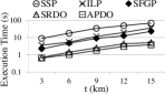
(a) Different algorithms.

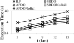
(b) Impact of BallTree.

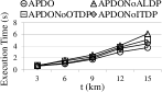
(c) Distance Pruning.

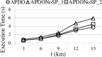
(d) Familiarity Pruning.

Figure 15: Performance comparisons on DataSet_4SQ.

Figures 15 evaluates the efficiency of MAGS on DataSet_4SQ. Figure 15(a) compares the computation time of the proposed algorithms with different values of $t$. Given its massive search space, SSP incurs the largest computation time as $t$ grows. On the other hand, equipped with Socio-Spatial Ordering, BallTree, Distance Pruning, and Familiarity Pruning, SRDO and APDO effectively reduce the time to acquire the optimal solution and outperform Integer Linear Programming (ILP). Moreover, APDO requires the minimum computation time because it can effectively minimize the total spatial distance from $S_{I}$ to $q_{ref}$ during each expansion of $S_{I}$. Figure 15(b) compares different algorithms with or without BallTree. Both SRDO and APDO require smaller computation time with BallTree and outperform ILP, since the proposed Outer-Triangle, Inner-Triangle and Activity Location Distance Pruning strategies are able to effectively remove redundant activity locations (within balls) at early stages.

Figures 15(c) and 15(d) present the impact of the proposed pruning strategies, i.e., Outer-Triangle Distance Pruning (OTDP), Inner-Triangle Distance Pruning (ITDP), Activity Location Distance Pruning (ALDP), and Familiarity Pruning shown in Eqs. (4) and (5) in Section 5.1 (denoted as SP_1 and SP_2). The results manifest that these pruning strategies effectively process the spatial and social relationships and indeed are critical for efficiently processing MRGQ. Moreover, the first Familiarity Pruning (SP_1) is more powerful than the second one (SP_2) since it derives a tighter upper bound on the number of people acquainted with each member in $S_{I}$.

7.3 Performance Evaluation of Proposed Algorithms for SSGQ

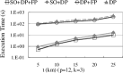
(a) Different strategies.

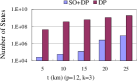
(b) Socio-Spatial Ordering.

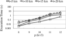
(c) Varying $p$.

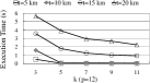
(d) Varying $k$.

Figure 16: Performance comparisons on DataSet_4SQ.

We set the spatial radius, $t$, as 10km in this set of experiments, which is determined based on the user study. The study indicates that most of the users are willing to participate in impromptu activities within 10km from them.

For SSGMerge, we empirically set $\lambda$ within the range $50\leq\lambda\leq 800$, because we observe that in this range, SSGMerge incurs small execution time while the obtained solutions achieve significant improvement over the straightforward approach, i.e., $i$-th feasible solution. On the other hand, $w$ should not be set too small, e.g., smaller than 10000, because the intermediate solutions in this case will not be able to include a sufficient number of distinct candidates, and thus limiting the possibility for constructing good solutions.

Figures 16(a) and 16(b) analyze the proposed strategies in Section 4, where SO, DP and FP denote Socio-Spatial Ordering, Distance Pruning and Familiarity Pruning, respectively. The result indicates that Socio-Spatial Ordering (SO) is effective in reducing the execution time. This is because Socio-Spatial Ordering considers both spatial and social domains and thereby is able to guide the efficient search of the feasible solutions and the optimal solution by exploring fewer states in the branch-and-bound tree, as shown in Figure 16(b).

Figures 16(c) and 16(d) compare SSGS with different parameter settings. Figure 16(c) indicates that the execution time increases as $p$ grows, because SSGS in this case needs to explore a larger search space to find the optimal solution. On the other hand, Figure 16(d) shows that a larger $k$ leads to a smaller execution time because it becomes easier to obtain feasible solutions for Distance Pruning to trim the search space.

7.4 Comparisons with ILP for SSGQ

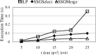
(a) Varying $t$.

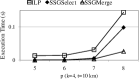
(b) Varying $p$.

Figure 17: Comparisons of the proposed algorithms with ILP for SSGQ.

Figure 17 compares the performance of Integer Linear Programming (ILP) with SSGMerge and SSGS. In our experiments, a renown general-purposed commercial parallel optimizer, CPLEX [1], is adopted to find the optimal solutions with the proposed ILP formulation, while both SSGMerge and SSGS are single-thread programs. ILP here represents a baseline benchmark for examining the efficiency of the proposed algorithms. Although SSGS and SSGMerge run in single-thread, they still outperform ILP. This is because SSGMerge and SSGS carefully include effective pruning and ordering strategies. Moreover, SSGMerge exploits the structure of intermediate solutions. Therefore, SSGMerge achieves superior performance over SSGS and ILP.

7.5 Performance Evaluation of SSGMerge

(a) Solution quality.

(b) Execution time.

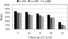
(c) Comparisons with OPT.

(d) Comparisons with SSGS.

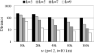
(e) Varying $w$.

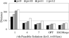
(f) Comparisons with the straightforward approach.

Figure 18: Experimental results of SSGMerge.

Figure 18 compares the solution quality and execution time of SSGMerge with different settings, and the default value of $w$ is set to 20k. In Figure 18(a) and 18(b), to compare the solution quality of SSGMerge and SSGS, we first measure the execution time of SSGMerge and then stop SSGS with the same length of time, and denote this solution as SSGTimeCut. Figure 18(a) shows the ratio between SSGTimeCut and SSGMerge, i.e., the total spatial distance of solutions obtained by SSGMerge divided by the total spatial distance of solutions obtained by SSGTimeCut, with different $\lambda$. When $\lambda$ increases, SSGMerge can obtain better solutions since it will examine more intermediate solutions and is more inclined to extract a better one. Moreover, when $t$ grows, the improvement from SSGMerge becomes more significant. This is because it becomes more difficult for SSGS to extract good feasible solutions at early stages, but SSGMerge can effectively merge existing intermediate solutions to obtain good solutions. Figure 18(b) shows the execution time of SSGMerge. When $t$ grows, the execution time increases slowly. This is because the size of the state sets is fixed and the extra computation of merging intermediate solutions incurred is thus limited.

Also, we compare the solutions returned by SSGMerge with the optimal solutions returned by SSGS in Figures 18(c) and 18(d). Figure 18(c) displays the ratio of the optimal solution and the solution obtained by SSGMerge, i.e., the optimal solution values divided by the solution values obtained by SSGMerge. The result manifests that the solutions obtained by SSGMerge are close to the optimal solution. Figure 18(d) compares the execution time of SSGMerge and SSGS, where SSGMerge outperforms SSGS and the execution time of SSGMerge increases very slowly when $t$ grows.

Figure 18(e) presents the solution quality of SSGMerge with different $w$. Here we set $\lambda$ as 200. The total spatial distance decreases when $w$ grows, because with a larger $w$, SSGMerge can examine more distinct candidate attendees in different intermediate solutions, which enables SSGMerge to construct better solutions.

In Figure 18(f), we compare the solution quality for different $p$ of SSGMerge and the straightforward approach with specified $i$, i.e., the $i$-th feasible solution in SSGS. We first measure the execution time of SSGS to obtain different feasible solutions and then set proper $\lambda$ to stop SSGMerge with the same length of time, while OPT represents the optimal solution returned by SSGS. Figure 18(f) shows that SSGMerge can obtain solutions which are close to the optimal solution and outperform the straightforward approach. Moreover, although the solutions obtained by the straightforward approach converge quickly when $i$ increases, SSGMerge can still obtain much better solutions. This is because SSGMerge each time combines a group with multiple attendees, which greatly reduces the time for expanding $S_{I}$ one by one. Moreover, Socio-Spatial Ordering ensures that the early expanded groups incur small total spatial distances. Therefore, SSGMerge can produce solutions which are close to the optimal solution.

7.6 Comparisons of MRGQ with Relevant Works

To compare with the state-of-the-art methods with different parameters, we have conducted more experiments by varying $k$, $|Q|$, and $p$. The results are presented in Figure 19. Figure 19(a) compares the feasibility ratio (i.e., the ratio of the obtained solutions satisfying the familiarity constraint) of MAGS and the other relevant approaches with different $k$. The proposed MAGS achieves 100% of feasibility ratio with different $k$ because the proposed Familiarity Pruning strategy effectively trims all the intermediate solutions that will not satisfy the familiarity constraint at an early stage. As $k$ decreases, the feasibility ratios of gCoFQ and pNN drop because pNN does not consider the social domain, while gCoFQ is designed to minimize a linear combination of the social diameter and spatial distance of the group members. It is worth noting that the feasibility ratio of pNN is low and unacceptable even with a loose familiarity constraint (i.e., $k=6$) because the groups returned by pNN are usually disconnected.

Figures 19(b) and 19(c) compare the solution quality and feasibility ratio of different approaches. When the number $|Q|$ of candidate locations increases, all approaches can find the solutions with smaller total spatial distances due to more potential good choices. Nevertheless, the proposed MAGS outperforms gCoFQ in terms of solution quality because gCoFQ does not examine activity locations but only tries to minimize the maximum spatial distance between each pair of group members. Although pNN acquires the groups with the minimum spatial distances, Figure 19(c) manifests that the feasibility ratio of pNN is very small because the individuals who are closest to an activity location do not satisfy the familiarity constraint in most cases.

Figure 19(d) presents the feasibility ratio with different $p$. Given the familiarity constraint $k=4$, the proposed MAGS always obtains the solutions satisfying the familiarity constraint (i.e., feasibility ratio is 100%). However, when $p$ increases, the feasibility ratios of gCoFQ and pNN drop. This is because more group members are necessary to be connected to each other when $p$ is larger, and it is thus more difficult for gCoFQ and pNN to follow the familiarity constraint. Moreover, although gCoFQ is able to obtain the groups with small social diameters, a few group members are still unacquainted with many other members. Therefore, the feasibility ratio of gCoFQ is still not sufficient.

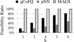
(a) Feasibility ratio of different $k$.

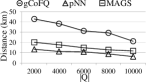
(b) Solution quality of different $|Q|$.

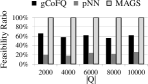
(c) Feasibility ratio of different $|Q|$.

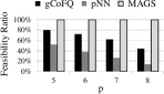
(d) Feasibility ratio of different $p$.

Figure 19: Comparisons with relevant works with different parameters.

7.7 Experimental Results for MAGS in Dynamic Environments

We perform experiments for MRGQ when the locations of the users are dynamically changing. We generate the user trajectories according to [22] as follows. We first extract from $DataSet\_4SQ$ the locations visited by each individual, and each individual is placed in one of its visited locations in equal probability with maximum speed of 0.75 km/min. The destination of each user is randomly picked from other visited locations. During the first $1/6$ of the route, users accelerate from zero speed to their maximum speeds. During the middle $2/3$ of the route, they travel at their maximum speeds; and in the last $1/6$ of the route, they decelerate. When a user reaches her destination, a new destination is assigned at random to her.

We compare MRGQs with R*-Tree [24] and TPR-Tree [22] in our experiments by changing the ratio of moving users (i.e., a specific ratio of users are moving, and the rest are static), and measure the number of index updates for MRGQs in the two index structures. In addition, query execution time measures the time to process each query with the two index structures. In our experiments, we issue MRGQs randomly at 30 different time slices within 90 minutes from the start time. The query parameters are set as $t=9km$, $p=8$, $k=4$, $|Q|=10000$, and $t_{f}=0$.

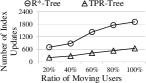
(a) Number of index updates.

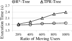
(b) Query execution time.

Figure 20: Comparisons of R*-Tree and TPR-Tree.

Figure 20(a) compares the number of index updates of R*-Tree and TPR-Tree with different ratios of moving users. As the ratio increases, the number of updates grows rapidly for R*-Tree. This is because when the number of moving users increases, more location updates occur, and R*-Tree updates the users locations, splits MBRs, and rebalances the index structure more frequently. In contrast, the number of index updates of TPR-Tree is small as compared to R*-Tree because TPR-Tree incorporates the velocity vectors for MBRs to avoid the frequent updates. Figure 20(b) compares the query execution time of R*-Tree and TPR-Tree with different ratios of moving users. Execution time of the MRGQs with R*-Tree and TPR-Tree are both small. The execution of MRGQs in R*-Tree is smaller than that in TPR-Tree because R*-Tree spends much time on updating the index structure and maintains smaller MBRs. The smaller MBRs in R*-Tree provide better index capability. In contrast, the execution time of TPR-Tree increases when the ratio of the number of moving users grows because in this case, the MBRs are larger and the index capability deteriorates.

7.8 Performance Comparisons for MAGS with Different Pruning Strategies

We compare SRDO, APDONoOTDP, APDONoITDP, APDONoALDP, and APDO by changing parameters $k$ and $p$. Figure 21 presents the experimental results with the default parameters $t=9$km, $p=8$, $k=4$, and $|Q|=10000$. When $k$ or $p$ increases, the computation time of APDO increases slowly. As shown, APDO outperforms the other approaches, i.e., APDONoALDP, APDONoOTDP, APDONoITDP, and SRDO because the proposed distance pruning strategies effectively avoid redundant activity location examinations. When $k$ increases, many approaches except APDO incur more computation time. This is because when $k$ becomes larger, Familiarity Pruning is less effective due to the loosen familiarity constraint. Nevertheless, the proposed APDO with all the distance pruning strategies is able to avoid redundant $S_{I}$ expansions. Similarly, when $p$ increases, the search space also increases. APDO with the pruning strategies can thus stop expanding $S_{I}$ earlier. Therefore, APDO outperforms the other approaches. Finally, APDO explores many possible $q_{ref}$ and $v_{c}$ during the expansion of $S_{I}$ to obtain good solutions much earlier than SRDO does. In other words, the distance pruning strategies in APDO is very effective, which enables the proposed APDO to significantly outperform SRDO.

(a) Distance pruning with different $k$ ($p=8$).

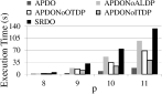
(b) Distance pruning with different $p$ ($k=4$).

Figure 21: Effectiveness of distance pruning strategies.

7.9 Experimental Results for MAGS on DataSet_Youtube

We evaluate the proposed MAGS on DataSet_Youtube, which is a social network extracted from Youtube video-sharing website with 1,134,890 individuals. Since there is no spatial information for this dataset, we randomly assign the spatial coordinates to the individuals as her current location. In our experiments, we randomly extract the activity locations from DataSet_4SQ. In the following experiments, unless specifically indicated, we set $k=4$, $p=8$, $|Q|=10,000$, and the maximum value of $t$ is 15 km.

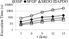
(a) Different algorithms.

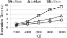
(b) Varying $|Q|$.

(c) Varying $k$.

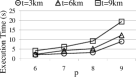
(d) Varying $p$.

Figure 22: Sensitivity tests of MAGS on DataSet_Youtube.

Figure 22 evaluates the proposed algorithms on DataSet_Youtube. Figure 22(a) shows that, although DataSet_Youtube contains about 8 times the number of candidates as DataSet_4SQ does, the computation time of SRDO and APDO both incur small computation time. This is because DataSet_Youtube is socially sparse (i.e., with an average degree 5.27), which enables the social pruning strategies to effectively remove redundant search space. Figures 22(b)-(d) compare APDO with different parameter settings. Since DataSet_Youtube contains fewer spatially dense clusters, the computation time is limited with the distance pruning strategies. Moreover, Familiarity Pruning is able to quickly prune unqualified groups due to the large number of low-degree nodes in the social graph, and the computation time is thus reduced.

8 Conclusion

To address the need of automatic activity planning based on the social and spatial relationships of attendees and activity locations, we define a new query, namely MRGQ, to jointly find the optimal set of attendees and the best activity location among multiple activity locations. We also study a special case of MRGQ, namely SSGQ, which only features a single activity location. We show that processing MRGQ is NP-hard and inapproximable within any factor. We formulate MRGQ with Integer Linear Programming and propose an efficient algorithm, namely MAGS. In addition to indexing the candidate attendees in R-Tree, we propose to index the candidate locations in BallTree, and devise various ordering and pruning strategies based on the social and spatial relationships. Experimental results show that the computation time required by single threaded MAGS is much smaller than using an IBM CPLEX parallel optimizer. Moreover, we show that the problem of processing SSGQ is NP-hard and devise an efficient algorithm, namely SSGS, to process SSGQ. Various strategies, including Distance Ordering, Socio-Spatial Ordering, Distance Pruning, and Familiarity Pruning are proposed to prune redundant search space and obtain the optimal solution efficiently. We also implement SSGQ in Facebook and conduct user studies for both SSGQ and MRGQ to demonstrate that the proposed algorithms significantly outperform manual coordination in terms of both solution quality and efficiency.

Appendix A Pseudo Codes of the Proposed Algorithms

The pseudo codes of the proposed algorithms, i.e., SSGS, SFGP, MAGS with Single-Reference Distance Ordering, and MAGS with All-Pair Distance Ordering, are presented as follows.

Algorithm 1 SSGS algorithm

1:Graph $G=(V,E)$, location $l_{v}$ for each $v\in V$, the number of attendees $p$, activity location $q$, familiarity constraint $k$, and spatial radius $t$. The user locations $l_{v},\forall v\in V$ are indexed by an R-Tree.

2:Optimal group $F$.

3:$S_{I}\leftarrow\varnothing$, $curDist\leftarrow 0$, $F\leftarrow\varnothing$, $D\leftarrow\infty$, $\theta\leftarrow k$

4:Employ R-Tree Range Query on $q$ to find the vertices within distance $t$ as $S_{R}$

5:FindGroup($S_{I}$,$S_{R}$,$curDist$)

6:if $D\neq\infty$ then

7:     output $F$

8:else

9:     output ”No Answer”

10:end if

11:procedure FindGroup($inS_{I}$,$inS_{R}$,$curDist$)

12:     $S_{I}\leftarrow inS_{I}$, $S_{R}\leftarrow inS_{R}$

13:     while $|S_{I}|+|S_{R}|\geq p$ do

14:         if there is any unvisited vertex in $S_{R}$ then

15:               Employ R-Tree distance browsing to extract from $S_{R}$ the next unvisited vertex $u$ which has the minimum spatial distance to $q$; mark $u$ as visited

16:         else if $\theta<p-1$ then

17:              increase $\theta$ and mark the remaining vertices in $S_{R}$ as unvisited

18:         else

19:              break

20:         end if

21:         if $u$ satisfies the condition of Socio-Spatial Ordering in Eq. (1) then

22:              $S_{I}\leftarrow S_{I}+\{u\}$, $S_{R}\leftarrow S_{R}-\{u\}$, $curDist\leftarrow curDist+d_{u,q}$

23:              if Familiarity Pruning in Eq. (2) or Distance Pruning in Eq. (3) is satisfied then

24:                  break

25:              else if $|S_{I}|<p$ then

26:                  FindGroup($S_{I}$,$S_{R}$,$curDist$)

27:              else

28:                  $D\leftarrow curDist$, $F\leftarrow S_{I}$

29:                  break

30:              end if

31:         else if $\theta=p-1$ then

32:              $S_{R}\leftarrow S_{R}-\{u\}$

33:         end if

34:     end while

35:end procedure

Algorithm 2 SFGP algorithm

1:Graph $G=(V,E)$, location $l_{v}$ for each $v\in V$, the number of attendees $p$, activity locations $Q$, familiarity constraint $k$, and spatial radius $t$. The user locations $l_{v},\forall v\in V$ are indexed by an R-Tree.

2:Optimal group $F$ and the corresponding activity location $q^{*}$

3:$S_{I}\leftarrow\varnothing$, $S_{R}\leftarrow V$, $Q_{I}\leftarrow Q$, $F\leftarrow\varnothing$, $D\leftarrow\infty$, $\theta\leftarrow k$

4: find $u\in S_{R}$ and $q_{ref}\in Q_{I}$ such that $u$ and $q_{ref}$ are the spatially closest pair

5:FindGroupAndLoc_SFGP($S_{I}$,$S_{R}$,$Q_{I}$,$q_{ref}$)

6:if $D\neq\infty$ then

7:     output $\langle F,q^{*}\rangle$

8:else

9:     output ”No Answer”

10:end if

11:procedure FindGroupAndLoc_SFGP($inS_{I}$,$inS_{R}$,$inQ_{I}$, $q_{ref}$)

12:     $S_{I}\leftarrow inS_{I}$, $S_{R}\leftarrow inS_{R}$, $Q_{I}\leftarrow inQ_{I}$

13:     while $|S_{I}|+|S_{R}|\geq p$ do

14:         if there is any unvisited vertex in $S_{R}$ then

15:               Employ R-Tree distance browsing to extract from $S_{R}$ the next unvisited vertex $u$ which has the minimum spatial distance to $q_{ref}$

16:              mark $u$ as visited

17:         else if $\theta<p-1$ then

18:              increase $\theta$ and mark the remaining vertices in $S_{R}$ as unvisited

19:         else

20:              break

21:         end if

22:         if $u$ satisfies the condition of Socio-Spatial Ordering in Eq. (1) then

23:              $S_{I}\leftarrow S_{I}+\{u\}$, $S_{R}\leftarrow S_{R}-\{u\}$

24:              if Familiarity Pruning in Eq. (4) or Eq. (5) is satisfied then

25:                  break

26:              end if

27:              for all $q_{i}\in Q_{I}$ do

28:                  if $S_{I}$ and $q_{i}$ satisfies Distance Pruning in Eq. (3) then

29:                       $Q_{I}\leftarrow Q_{I}-\{q_{i}\}$

30:                  else if $d_{v,q_{i}}>t$ then

31:                       $Q_{I}\leftarrow Q_{I}-\{q_{i}\}$

32:                  end if

33:              end for

34:              if $Q_{I}=\varnothing$ then

35:                  break

36:              end if

37:              if $|S_{I}|<p$ then

38:                  FindGroupAndLoc_SFGP($S_{I}$,$S_{R}$,$Q_{I}$,$q_{ref}$)

39:              else

40:                  if $\min_{q_{i}\in Q_{I}}\sum_{v\in S_{I}}d_{v,q_{i}}<D$ then

41:                       $q^{*}\leftarrow\arg\min_{q_{i}\in Q_{I}}\sum_{v\in S_{I}}d_{v,q_{i}}$

42:                       $D\leftarrow\sum_{v\in S_{I}}d_{v,q^{*}}$, $F\leftarrow S_{I}$

43:                  end if

44:                  break

45:              end if

46:         else if $\theta=p-1$ then

47:              $S_{R}\leftarrow S_{R}-\{u\}$

48:         end if

49:     end while

50:end procedure

Algorithm 3 MAGS algorithm with APDO

1:Graph $G=(V,E)$, location $l_{v}$ for each $v\in V$, the number of attendees $p$, activity locations $Q$, familiarity constraint $k$, and spatial radius $t$. The user locations $l_{v}\in V$ are indexed by an R-Tree with root $M_{0}$. The activity locations $q_{i}\in Q$ are indexed by a BallTree with root $B_{0}$.

2:Optimal group $F$ and the corresponding activity location $q^{*}$

3:$S_{I}\leftarrow\varnothing$, $S_{R}\leftarrow V$, $Q_{I}\leftarrow Q$, $F\leftarrow\varnothing$, $D\leftarrow\infty$, $\theta\leftarrow k$

4:$\langle F,q^{\ast}\rangle\leftarrow$ FindGroupAndLoc_APDO($S_{I}$,$S_{R}$,$Q_{I}$,$B_{0}$)

5:if $D\neq\infty$ then

6:     output $\langle F,q^{*}\rangle$

7:else

8:     output ”No Answer”

9:end if

10:procedure FindGroupAndLoc_APDO($inS_{I}$,$inS_{R}$,$inQ_{I}$,$inB_{0}$)

11:     $S_{I}\leftarrow inS_{I}$, $S_{R}\leftarrow inS_{R}$, $Q_{I}\leftarrow inQ_{I}$, $B_{0}\leftarrow inB_{0}$

12:     while $|S_{I}|+|S_{R}|\geq p$ do

13:         if there is any unvisited vertex in $S_{R}$ then

14:              $\langle v_{c}$,$q_{ref}\rangle\leftarrow$ APDOandDistPruning($M_{0}$,$B_{0}$,$S_{I}$,$S_{R}$,$Q_{I}$), $u\leftarrow v_{c}$

15:               let $Q_{I}$ be the set of leaf nodes in BallTree which are neither pruned nor the descendants of a pruned ball

16:              mark $u$ as visited

17:         else if $\theta<p-1$ then

18:              increase $\theta$ and mark the remaining vertices in $S_{R}$ as unvisited

19:         else

20:              break

21:         end if

22:         if $u$ satisfies the condition of Socio-Spatial Ordering in Eq. (1) then

23:              $S_{I}\leftarrow S_{I}+\{u\}$, $S_{R}\leftarrow S_{R}-\{u\}$

24:              if Familiarity Pruning in Eq. (4) or Eq. (5) is satisfied then

25:                  break

26:              end if

27:              for all $q_{i}\in Q_{I}$ do

28:                  if $S_{I}$ and $q_{i}$ satisfies Distance Pruning in Eq. (3) then

29:                       mark $q_{i}$ as pruned, $Q_{I}\leftarrow Q_{I}-\{q_{i}\}$

30:                  else if $\exists v\in S_{I}$ such that $d_{v,q_{i}}>t$ then

31:                       mark $q_{i}$ as pruned, $Q_{I}\leftarrow Q_{I}-\{q_{i}\}$

32:                  end if

33:              end for

34:              if $Q_{I}=\varnothing$ then

35:                  break

36:              end if

37:              if $|S_{I}|<p$ then

38:                  FindGroupAndLoc_APDO($S_{I}$,$S_{R}$,$Q_{I}$,$B_{0}$)

39:              else

40:                  if $\min_{q_{i}\in Q_{I}}\sum_{v\in S_{I}}d_{v,q_{i}}<D$ then

41:                       $q^{*}\leftarrow\arg\min_{q_{i}\in Q_{I}}\sum_{v\in S_{I}}d_{v,q_{i}}$

42:                       $D\leftarrow\sum_{v\in S_{I}}d_{v,q^{*}}$, $F\leftarrow S_{I}$

43:                  end if

44:                  break

45:              end if

46:         else if $\theta=p-1$ then

47:              $S_{R}\leftarrow S_{R}-\{u\}$

48:         end if

49:     end while

50:end procedure

APDOandDistPruning

1:procedure APDOandDistPruning($M_{0}$,$B_{0}$,$S_{I}$,$S_{R}$,$Q_{I}$)

2:     let $U_{R}$ and $U_{B}$ be two lists

3:     $M\leftarrow M_{0}$, $B\leftarrow B_{0}$

4:     $U_{R}\leftarrow M_{0}$, $U_{B}\leftarrow B_{0}$

5:     $v_{c}\leftarrow\varnothing$, $q_{ref}\leftarrow\varnothing$

6:     while $M$ and $B$ are not both leaf nodes do

7:          pop MBR $M_{i}$ from $U_{R}$ and pop ball $B_{j}$ from $U_{B}$ such that $\sum_{v\in S_{I}}MINDIST(v,B_{j})+MINDIST(M_{i},B_{j})$ is minimum, and $B_{j}$ is not pruned

8:         $M\leftarrow M_{i}$, $B\leftarrow B_{j}$

9:         if $M$ and $B_{x}\leftarrow B$ satisfy OTDP Lemma 2 and prune $B_{y}$ in $U_{B}$ then

10:              remove $B_{y}$ from $U_{B}$, mark $B_{y}$ as pruned

11:         else if ITDP in Lemma 4 prunes $B_{x}$ in $U_{B}$ then

12:              remove $B_{x}$ from $U_{B}$, mark $B_{x}$ as pruned

13:         else if ALDP in Lemma 5 prunes $B_{x}$ in $U_{B}$ then

14:              remove $B_{x}$ from $U_{B}$, mark $B_{x}$ as pruned

15:         end if

16:         if $M$ is not a leaf node then

17:              for all child MBR $M_{i}$ of $M$ do

18:                  if $M_{i}$ contains $l_{v}$ where $v\in S_{R}$ then

19:                       push $M_{i}$ into $U_{R}$

20:                  end if

21:              end for

22:         end if

23:         if $B$ is not a leaf node then

24:              for all child ball $B_{j}$ of $B$ do

25:                  push $B_{j}$ into $U_{B}$

26:              end for

27:         end if

28:     end while

29:     $v_{c}\leftarrow M$, $q_{ref}\leftarrow B$

30:     return $\langle v_{c}$,$q_{ref}\rangle$

31:end procedure

References

-
[1]
CPLEX.
http://www-01.ibm.com/software/integration/
optimization/cplex-optimizer/. - [2] N. Roussopoulos, S. Kelley and F. Vincent. Nearest Neighbor Queries. SIGMOD, 1995.
- [3] T. Lappas, K. Liu, and E. Terzi. Finding a Team of Experts in Social Networks. KDD, 2009.
- [4] C.-T. Li and M.-K. Shan. Team Formation for Generalized Tasks in Expertise Social Networks. SocialCom, 2010.
- [5] M. Sozio and A. Gionis. The Community-Search Problem and How to Plan a Successful Cocktail Party. KDD, 2010.
- [6] D. Papadias, Q. Shen, Y. Tao and K. Mouratidis. Group Nearest Neighbor Queries. ICDE, 2004.
- [7] Y. Tao, D. Papadias and Q. Shen. Continuous Nearest Neighbor Search. VLDB, 2002.
- [8] D.-N. Yang, Y.-L. Chen, W.-C. Lee and M.-S. Chen. On Social-Temporal Group Query with Acquaintance Constraint. VLDB, 2011.
- [9] W. Liu, W. Sun, C. Chen, Y. Huang, Y. Jian and K. Chen. Circle of Friend Query in Geo-Social Networks. DASFAA, 2012.
- [10] Y. Gao, B. Zheng, W.-C. Lee, G. Chen. Continuous Visible Nearest Neighbor Queries. EDBT, 2009.
- [11] Y. Gao and B. Zheng. Continuous Obstructed Nearest Neighbor Queries in Spatial Databases. SIGMOD, 2009.
- [12] G. Hjaltason and H. Samet. Distance Browsing in Spatial Databases. TODS, 1999.
- [13] W. Liu, W. Sun, C. Chen, Y. Huang, Y. Jian and K. Chen. Circle of Friend Query in Geo-Social Networks. DASFAA, 2012.
- [14] S. Omohundro. Five Balltree Construction Algorithms. Technical Report, 1989.
- [15] N. Mahadev and U. Peled. Threshold Graphs and Related Topics. Elsevier, 1995.
- [16] D. Liu and X. Zhu. Circular Distance Two Labeling and the -Number for Outerplanar Graphs. SIAM J. Discrete Math, 2005.
- [17] G. Chang and D. Kuo. The -Labeling Problem on Graphs. SIAM J. Discrete Math, 1996.
- [18] S. Seidman. Network Structure and Minimum Degree. Social Networks, 1983.
- [19] V. Batagelj and M. Zaversnik. An Algorithm for Core Decomposition of Networks. CoRR, 2003.
- [20] M. Ye, P. Yin, W.-C. Lee and D.-L. Lee. Exploiting Geographical Influence for Collaborative Point-of-Interest Recommendation. SIGIR, 2011.
- [21] J. Yang and J. Leskovec. Defining and Evaluating Network Communities based on Grouth-truth. ICDM, 2012.
- [22] S. Saltenis, C. Jensen, S. Leutenegger, and M. Lopez. Indexing the Positions of Continuously Moving Objects. SIGMOD, 2000.
- [23] Y. Tao, D. Papadias, and J. Sun. The TPR*-tree: an Optimized Spatiotemporal Access Method for Predictive Queries. VLDB, 2002.
- [24] N. Beckmann, P. Kriegel, R. Schneider, and B. Seeger. The R*-tree: an Efficient and Robust Access Method for Points and Rectangles. SIGMOD, 1990.