CERN-PH-TH-2015-110 U(1) lattice gauge theory with a topological action

Abstract

We investigate the phase diagram of the compact $U(1)$ lattice gauge theory in four dimensions using a non-standard action which is invariant under continuous deformations of the plaquette angles. Just as for the Wilson action, we find a weakly first order transition, separating a confining phase where magnetic monopoles condense, and a Coulomb phase where monopoles are dilute. We also find a third phase where monopoles are completely absent. The topological action offers an algorithmic advantage for the computation of the free energy.

I Introduction

In recent years lattice Quantum Field Theory has seen a surge of efforts to construct new lattice actions which aim at improving the approach to the continuum limit. The best-known strategy is that advocated by Symanzik, where irrelevant operators of higher and higher dimension are added to the “standard” (e.g. Wilson plaquette) action, with coefficients adjusted perturbatively or non-perturbatively to cancel discretization errors of the corresponding power in the lattice spacing $a$ Symanzik (1983); Weisz (1983). This kind of improvement is thus a parametric one, allowing for a faster approach to the continuum limit than exhibited by the “standard” action.

However, this is not the only possible strategy for improvement. It has long been recognized that departure from the continuum limit is more violent for large fields, so that suppressing these large fields produces a non-parametric improvement Meurice (2002). For instance, this happens when one trades the Wilson action for the Manton action Michael and Teper (1988), based on the length of the geodesic in group space, or for a “perfect” action Rufenacht and Wenger (2001): large fields, corresponding to small values of the plaquette trace, are more suppressed than with the Wilson action, and at the same time continuum behavior is better approximated for a given value of the lattice spacing $a$.

A more radical suppression of large fields is achieved by imposing a strict cutoff: for instance, in a spin model one can demand that neighboring spin angles do not differ by more than a limiting value; or in a gauge theory, one may require that the plaquette trace be larger than a limiting value. The best-known example of the latter is the positive-plaquette action for $SU(2)$ lattice gauge theory Mack and Pietarinen (1982); Bornyakov et al. (1991); Fingberg et al. (1995). While the approach to the continuum limit is also improved in this strategy, an important side-effect may happen. Localized topological defects can only form if the cutoff is not too restrictive. For instance, an $O(2)$ spin model on a square lattice can support vortices only if the spins can rotate by $\pi/2$ or more between neighboring sites. If not, the disordered phase of this system disappears entirely. Thus, the cutoff may change the phase diagram of the model. A similar situation occurs in lattice gauge theory: as pointed out by Lüscher Luscher (1982), if the plaquette trace is restricted to “admissible” values greater than about 0.97 (for $SU(2)$), changes in the topological charge become impossible, and topology becomes well defined on the lattice. Topological sectors arise as in the continuum theory.

Here, we consider the extreme strategy where the action consists only of a cutoff. In other words, the action takes only two values: 0 if all cutoff restrictions are satisfied, $+\infty$ if not. This kind of action has been called topological Bietenholz et al. (2010), because it does not have any classical small-$a$ limit, and the action remains invariant under small admissible deformations of the field. A simple example of topological action for an $O(N)$ spin model is:

$$S=\sum_{\left\langle i,j\right\rangle}R_{\theta}(S_{i}\cdot{}S_{j}),\;\;R_{\theta}(x)=\begin{cases}0&x>\cos\theta\\ +\infty&\text{else}\end{cases}.$$ (1)

Topological actions raise an interesting puzzle: as the constraint between neighboring spins becomes more restrictive, the correlation length increases and diverges; but what is the action associated with this continuum limit? Several studies have investigated different spin models Bietenholz et al. (2010, 2013), and it has been shown in analytically solvable $O(N)$ models that the continuum limit is that associated with the usual, sigma-model action. In higher dimensions numerical investigations also support this claim very strongly.

Here we want to investigate the properties of a topological action in a gauge theory, and consider the simplest case, namely compact $U(1)$ lattice gauge theory in 4 dimensions. Aside from the continuum limit, we also want to study the phase diagram of this system. With the Wilson action, a first-order phase transition separates a strong-coupling, confining phase and a weak-coupling Coulomb phase. This phase transition is associated with condensation of magnetic monopoles in the strong-coupling phase DeGrand and Toussaint (1980). With a topological action, the constraint on the plaquette trace, when restrictive enough, is going to make it impossible for magnetic monopoles to exist. This may completely alter the phase diagram of the theory.

Finally, topological actions may be interesting for algorithmic reasons: it may be computationally easier to move in the space of admissible configurations since they all have the same action. While this promise has not yet been realized for the Monte Carlo update of such configurations, in spin models or in the gauge theory we study, we show below that extracting the free energy (or equivalently here, the entropy) is extremely simple numerically, and yields valuable information.

Our paper is organized as follows: we discuss the topological action of our model in Sec. II, the consequences for magnetic monopoles in Sec. III, the helicity modulus in Sec. IV, propose some arguments about the continuum limit in Sec. V, and discuss how to obtain the free energy in Sec. VI. Our results on the phase diagram are presented in Sec. VII, followed by conclusions.

II The action

The obvious analogue of restricting the angles between neighboring spins in a spin model is to restrict the real part of the trace of each plaquette in a gauge theory. The action then depends on one coupling $\alpha$ and is given by

$$e^{-S}=\begin{cases}1&\mathrm{ReTr}U_{P}>\alpha\quad\forall P\\ 0&\text{else}\end{cases},$$ (2)

where $P$ denotes a plaquette. Note that this formulation is independent of the gauge group but that we from now on consider only $U(1)$ where $\mathrm{ReTr}U_{P}=\cos\theta_{P}$. We could thus equally well consider a restriction of the plaquette angle $\theta_{P}$ with $\lvert\theta_{P}\mod 2\pi\rvert<\delta_{\text{max}}\equiv\arccos\alpha$. It is also important to note that the link angles, being gauge variant, are completely unrestricted. The most efficient way to generate configurations is to apply heatbath updates to the links one at a time under the constraint that no plaquette angle exceeds the allowed value. In principle this is realized by just uniformly sampling the interval $[0,2\pi]$ until an acceptable angle has been found but in some cases it might be more efficient to explicitly construct the allowed range of values for the link to be updated. Note that a Metropolis update based on the old value may not be ergodic since the admissible region of link angles may not be connected. See Fig. 1. However, there are some additional caveats to this kind of single link update which will become clear in the discussion of the magnetic monopoles.

Figure 1: Forbidden regions (hatched areas) and allowed regions (black lines) for the angle of a link surrounded by three (the others are omitted for clarity) staples $s_{i}$. When the restriction angle $\delta_{\text{max}}>\pi/2$ (left panel) the region can be disconnected whereas if it is smaller than $\pi/2$ (right panel) it will always be connected. $\delta_{\text{max}}$ is the angle between an arrow and the edge of the hatched area opposite to it.

III Magnetic monopoles

An elementary cube on the lattice contains $q$ magnetic monopoles if the outward oriented, physical ($\theta_{P}\in[-\pi,\pi[$) plaquette angles of its faces sum up to $2\pi q$ DeGrand and Toussaint (1980). It is easy to check that $q\in\{0,\pm 1,\pm 2\}$ and that a cube with $q$ monopoles must have at least one face with physical plaquette angle $\lvert\theta_{P}\rvert\geq\lvert q\rvert\pi/3$. This immediately tells us that for $\delta_{\text{max}}<\pi/3$ there cannot be any monopoles and the topological action does not describe the same (lattice) physics as the Wilson action . In fact, a change of variables from link to rescaled plaquette angles $\theta_{P}/\delta_{\text{max}}$ can be used to see that all $\delta_{\text{max}}<\pi/3$ are equivalent up to trivial rescalings. Let us therefore concentrate on angles larger than that.

One might think that if there is a deconfinement transition at some restriction angle $\delta_{\text{max}}$ then it should be at $\delta_{\text{max}}=\pi/3$ since this angle separates the region of no monopoles from a region with monopoles. This turns out to be wrong. In a sense this is analogous to the situation with the Wilson action. At the deconfinement transition the monopole density jumps down, but it does not jump to zero. The system can sustain a small density of monopoles without being confining. The same happens for the topological action with a deconfinement transition at a significantly larger restriction angle than $\pi/3$. Still, there is a non-analyticity in the monopole density at $\delta_{\text{max}}=\pi/3$, which we investigate further in Sec. VII (see Figs. 9 and 10).

III.1 Creating monopoles

To study how the monopoles depend on the cutoff angle $\delta_{\text{max}}$ it is important to understand what the lowest monopole excitation is. It is well known that every monopole is connected to an anti-monopole via a Dirac string and that the monopole worldlines must form closed loops on the dual lattice. The shortest such loop has four vertices and Euclidean length $2\sqrt{2}a$ where $a$ is the lattice spacing, and the smallest excitation is thus two monopoles and two anti-monopoles each located in one of the four cubes sharing a single plaquette. See Fig. 2 for an illustration.

Figure 2: The smallest possible nontrivial loop of monopoles world lines which has Euclidean length $2\sqrt{2}a$. The $y$ and $z$ dimensions are collapsed into one so that each cube is represented by a plaquette and each plaquette by a link. The fat link represents the plaquette shared by all four cubes which contain a monopole. A $+(-)$ in a plaquette symbolizes a positively(negatively) charged monopole in the corresponding cube.

It is also important to consider how such a configuration is created from a configuration with zero monopoles. In order to create a monopole in a given cube we need to change its flux by $2\pi$ at the same time as we respect the constraints on the plaquette angles. It is therefore relevant to investigate the smallest constraint angle for which a change of $2\pi$ in the flux is possible. If we update a single edge of a cube we will change two of its six plaquettes. The sum of these changes must be $2\pi$ and the required angles can be minimized by letting the change be distributed equally over all involved plaquettes. Hence, the restriction on the plaquette angles gives $\delta_{\text{max}}>\pi/2$ to create a monopole with a single link update. This means that for $\pi/2>\delta_{\text{max}}>\pi/3$ the single link update is not ergodic and cannot be used on its own. To have an ergodic algorithm we need to update at least three faces of a cube at the same time, which can only be done by updating more than one link at a time, as illustrated in Fig. 3. The minimal update to achieve this is shown in the lower part of Fig. 3 where two links of a given plaquette are updated together. This update changes three plaquettes in each of the four cubes sharing the plaquette common to the two updated links, and we thus have a chance to create four monopoles down to $\delta_{\text{max}}=\pi/3$ as required.

Figure 3: Monopole creation with a single link update (upper panel) and a multiple link update (lower panel). The fat links are the ones updated and the flux of $\pi$ is spread over the plaquettes on the right which means that the single link update is ergodic down to $\delta_{max}=\pi/2$ and the two-link one to $\pi/3$.

IV The Helicity modulus

The helicity modulus was first introduced in the $2d$ $XY$-model Nelson and Kosterlitz (1977) where it quantifies the response of the system to a twist in the boundary conditions. Because the twist is a boundary effect the helicity modulus is an order parameter for a system with one massive (finite correlation length) and one massless (infinite correlation length) phase. This is precisely the case of $4d$ lattice $U(1)$ gauge theory where the confining phase features massive photons whereas they are massless in the Coulomb phase. In the context of a gauge theory the twisted boundary conditions can also be thought of as an external electromagnetic flux Vettorazzo and de Forcrand (2004). More precisely, we define the helicity modulus as

$$h\equiv\left.\frac{\partial^{2}f(\phi)}{\partial\phi^{2}}\right\rvert_{\phi=0},$$ (3)

where $f$ is the free energy density in the presence of the external flux $\phi$. The flux is introduced by the replacement

$$\cos(\theta_{P})\to\cos(\theta_{P}+\phi)$$ (4)

for all plaquettes in a given stack of plaquettes, i.e. all plaquettes in the set $\{P_{\mu\nu}(x)\mid\mu=\mu_{0},\nu=\nu_{0};x_{\mu}=x_{0},x_{\nu}=y_{0}\}$. The orientation and position of the pierced stack is arbitrary and with a suitable change of variables the flux can also be spread out evenly over the $(\mu_{0},\nu_{0})$-planes. For the Wilson action $h$ is a simple difference of expectation values

$$h=\beta\left(\left\langle\cos\theta_{P}\right\rangle-\beta\left\langle\left(\sum_{\text{stack}}\sin\theta_{P}\right)^{2}\right\rangle\right),$$ (5)

where the sum in the second term is over all plaquettes in the stack defined above. For the topological action on the other hand, it is not possible to explicitly perform the derivatives. However, since the action for each configuration is the same, the free energy is given solely by the entropy, i.e. by the number of configurations with a given flux $\phi$. This can be measured by promoting the flux to a dynamical variable, which is updated along with the link angles Bietenholz et al. (2013). By measuring the probability distribution $p(\phi)$ (via a histogram method for example) of the visited fluxes one thus obtains the full $2\pi$ periodic free energy Vettorazzo and de Forcrand (2004) and the helicity modulus

$$h=-\left.\frac{\partial^{2}\log p(\phi)}{\partial\phi^{2}}\right\rvert_{\phi=0}.$$ (6)

Alternatively, and more accurately, one can use all the global information from $p(\phi)=e^{-f(\phi)}$ and fit it to the classical ansatz Vettorazzo and de Forcrand (2004)

$$f(\phi) =-\log\sum_{k}e^{-\frac{\beta_{R}}{2}\left(\phi-2\pi k\right)^{2}}$$

$$=-\log\vartheta_{3}\left(\frac{\phi}{2};e^{-\frac{1}{2\beta_{R}}}\right)-\frac{1}{2}\log 2\pi\beta_{R},$$ (7)

where $\beta_{R}$ plays the role of the renormalized coupling in the Coulomb phase and $\vartheta_{3}(z,q)$ is a Jacobi theta function. From this ansatz we can extract the curvature at $\phi=0$, i.e. $h$, analytically and we thus obtain both the helicity modulus and the renormalized coupling at the same time. We further note that they approach each other exponentially fast for large $\beta_{R}$. Together with eq. (5) we see that this means that $\beta_{R}\approx h\to\beta-1/4$ as $\beta\to\infty$, which is to say that the coupling constant is not renormalized in the continuum limit which is of course common knowledge.

V Continuum limit

It is important to dwell a little on the matter of a continuum limit for the topological action. Since all the plaquettes are forced to unity when $\delta_{\text{max}}\to 0$ one expects that in this limit the correlation length diverges and thus that it defines a continuum limit. This point of view was examined more thoroughly by Budczies and Zirnbauer in Budczies and Zirnbauer (2003). These authors consider a general weight function $w_{t}(U_{P})$, which is a function of a plaquette variable $U_{P}$ and some parameter (coupling) $t$. Granted that there exists a $t_{c}$ such that $w_{t_{c}}(U_{P})=\delta(U_{p}-\text{id})$ and that for $t\neq t_{c}$ the weight function is some smeared version of the $\delta$-function, then the lattice gauge theory with partition function

$$Z_{t}=\int\mathrm{d}[U]\,\prod_{P}w_{t}(U_{P})$$ (8)

has a continuum limit as $t\to t_{c}$. Furthermore, the authors claim that under “favorable conditions”, the continuum theory will be Yang-Mills theory. It is not precisely defined what conditions are considered favorable, but close to the identity element, the plaquette variable is well approximated by $U_{P}=e^{ia^{2}F_{P}}\approx 1+ia^{2}F_{P}-a^{4}F_{P}^{2}$. Thus, in order for the continuum action to be $\propto\int\text{Tr}F^{2}$ the weight function $w_{t}$ certainly has to satisfy some conditions on the moments of the tangent vectors of the Lie group. At the very least the first moment must vanish and the second moment needs to exist and have the correct sign. The authors indeed give an example in Budczies and Zirnbauer (2003) of a weight function, in two dimensions and for gauge group U$(N)$, which satisfies the $\delta$-function condition but which has the wrong continuum limit. The problem is identified with the non-existence of the second moment for the considered weight function.

The topological action which we use clearly satisfies the $\delta$-function constraint since the weight function has support only on a compact region of width $\pm\delta_{\text{max}}$ around the identity element and thus goes to $\delta(U_{P}-\text{id})$ as $\delta_{\text{max}}\to 0$. Because of the compact support and invariance under Hermitian conjugation we also conclude that the first moment vanishes and that the second is positive as it should. It is therefore probable that this action will have the correct quantum continuum limit and indeed all numerical evidence suggests that it does.

A simple check one can perform is to use for $w_{t}(U_{P})$ a combination of angle restriction and Wilson plaquette term with negative $\beta$. By taking $\delta_{\text{max}}\to 0$ the action still satisfies the $\delta$-function constraint but the negative value of $\beta$ will try to bend the distribution in the wrong direction to make the second moment of $w_{t}$ negative. Clearly, for a fixed value of $\beta$ the action will still be almost flat as long as $\delta_{\text{max}}$ is small enough, so in order to change the continuum limit, $\beta$ needs to be taken to $-\infty$ at the same time as $\delta_{\text{max}}\to 0$. Then, if the magnitude of $\beta$ is large enough we expect that the continuum limit is spoiled. This can also be observed in numerical simulations, and although it is somewhat of a pathological example it still gives some insight as to when one can expect to obtain the correct continuum limit.

VI Free energy

Here, we show how to evaluate the free energy, analytically in a $1d$ toy model, and numerically for more realistic cases.

VI.1 $1d$ $XY$ model

Consider a periodic chain of $N$ spins $s_{i}\in{}O(2)$ with a topological action which restricts the angle of each link $\ell_{i}=s_{i}s^{\dagger}_{i+1}$ to be smaller than $\delta_{\text{max}}$. Let $\ell_{i}=\exp(i\theta_{i}),\;\theta_{i}\in[-\delta_{\text{max}},\delta_{\text{max}}]$. The partition function of this model then takes a very simple form,

$$Z=\int\limits_{-\delta_{\text{max}}}^{\delta_{\text{max}}}\prod_{i=1}^{N}\frac{\mathrm{d}\theta_{i}}{2\delta_{\text{max}}}\delta\left(\exp\left(i\sum_{i=1}^{N}\theta_{i}\right)-1\right)$$ (9)

and describes a collection of $N$ non-interacting, constrained links with the only condition that the product of all links is one. The normalization of the angle integrals serves to keep $Z$ finite as the number of links is taken to infinity and is just a subtraction of the ground state energy.

The total angle can take values $2\pi m,\;m\in\{-\left\lfloor\frac{N\delta_{\text{max}}}{2\pi}\right\rfloor,\ldots,\left\lfloor\frac{N\delta_{\text{max}}}{2\pi}\right\rfloor\}$ and thus $m$ is the winding number or topological charge of the system. The partition function can be expressed solely in terms of the total angle by convoluting the uniform distributions of the individual links $N$ times. The distribution of the sum of $N$ i.i.d. uniform variables converges very rapidly to the normal distribution, in this case with zero mean and variance $N\delta_{\text{max}}^{2}/3$. Anticipating the $N\to\infty$ limit we thus neglect the small deviations from the normal distribution and write

$$Z =\sqrt{\frac{3}{2\pi N\delta_{\text{max}}^{2}}}\int\limits_{-N\delta_{\text{max}}}^{N\delta_{\text{max}}}\!\!\!\!\!\!\!\!\mathrm{d}\theta\,\exp\left(-\frac{3\theta^{2}}{2N\delta_{\text{max}}^{2}}\right)\delta\left(\exp\left(i\theta\right)-1\right)$$

$$=\frac{\sqrt{3}}{(2\pi)^{3/2}\alpha}\sum_{m=-\left\lfloor\sqrt{N}\alpha\right\rfloor}^{\left\lfloor\sqrt{N}\alpha\right\rfloor}\exp\left(-\frac{3}{2}\left(\frac{m}{\alpha}\right)^{2}\right),$$ (10)

where we have defined $\alpha\equiv\frac{\sqrt{N}\delta_{\text{max}}}{2\pi}$. We can now take $N\to\infty$ whilst keeping $\alpha$ fixed to obtain

$$Z =\frac{\sqrt{3}}{(2\pi)^{3/2}\alpha}\sum_{m=-\infty}^{\infty}\exp\left(-\frac{3}{2}\left(\frac{m}{\alpha}\right)^{2}\right)$$

$$=\frac{\sqrt{3}}{(2\pi)^{3/2}\alpha}\vartheta_{3}\left(\exp\left(-\frac{3}{2\alpha^{2}}\right)\right),$$ (11)

where $\vartheta_{3}(q)\equiv\vartheta_{3}(0,q)$ is the third Jacobi elliptic theta function. Since the sum in the partition function is over the winding number $m$ it is straightforward to calculate $\left\langle m^{2}\right\rangle$ and the topological susceptibility $\chi_{t}=\frac{1}{\beta}\left\langle m^{2}\right\rangle$. In the limit $\beta=Na\propto\alpha^{2}\to\infty$ (where $a$ is the lattice spacing) one should find $\chi_{t}=\frac{1}{4\pi^{2}I}$ where $I$ is the moment of inertia of the quantum rotor which the model describes. This allows us to determine $\alpha$ in terms of $\beta$ and $I$ and the result is $\alpha=\frac{\sqrt{3\beta/I}}{2\pi}$ which leads to

$$Z=\sqrt{\frac{I}{2\pi\beta}}\vartheta_{3}\left(\exp\left(-\frac{2\pi^{2}I}{\beta}\right)\right).$$ (12)

With Poisson’s summation formula we can go from the winding number representation to the energy representation in which

$$Z=\vartheta_{3}\left(\exp\left(-\frac{\beta}{2I}\right)\right)=\sum_{k=-\infty}^{\infty}\exp\left(-\frac{k^{2}\beta}{2I}\right).$$ (13)

It is now evident that the excited states are doubly degenerate and the energy differences are $E_{k}-E_{0}=\frac{k^{2}}{2I}$ as is well known. The topological susceptibility is given in the two representations by

$$\chi_{t} =\frac{\exp\left(-\frac{2\pi^{2}I}{\beta}\right)\vartheta^{\prime}_{3}\left(\exp\left(-\frac{2\pi^{2}I}{\beta}\right)\right)}{\beta\vartheta_{3}\left(\exp\left(-\frac{2\pi^{2}I}{\beta}\right)\right)}$$

$$=\frac{1}{4\pi^{2}I}\left(1-\beta\frac{\exp\left(-\frac{\beta}{2I}\right)\vartheta^{\prime}_{3}\left(\exp\left(-\frac{\beta}{2I}\right)\right)}{\vartheta_{3}\left(\exp\left(-\frac{\beta}{2I}\right)\right)}\right).$$ (14)

Since the elliptic function and its derivative are analytic functions $\forall\beta\in\mathbb{R}^{+}$ there is no phase transition but there are two distinct regimes with a rather abrupt crossover. In the low temperature regime, $\beta/I\gtrsim 10$, the partition function is almost independent of $\beta$ and the topological susceptibility is very close to its zero temperature value $(4\pi^{2}I)^{-1}$ whereas in the high temperature region, $\beta/I\lesssim 10$, the partition function is approximately $\sqrt{2\pi\beta}$ and $\chi_{t}$ rapidly drops to zero.

Note that, when $N\delta_{\text{max}}<2\pi$, topological excitations are forbidden and $\chi_{t}=0$. However, the continuum limit is obtained while keeping $(N\delta_{\text{max}}^{2}$ fixed, so that the lattice spacing varies $\propto\delta_{\text{max}}^{2}$. Therefore, in this $1d$ model the parameter region where $\chi_{t}=0$ disappears in the continuum limit.

VI.2 Higher dimensions and gauge theories

In higher dimensions, due to the lattice Bianchi identities, the integration over the constrained variables no longer factorizes and we can not calculate the partition function analytically anymore. However, in the small $\delta_{\text{max}}$ regime where there are no topological defects the partition function must be

$$Z=\left(2\delta_{\text{max}}\right)^{n_{\text{d.o.f}}}$$ (15)

(or one, depending on the normalization), where $n_{\text{d.o.f}}$ is the number of independent degrees of freedom. As the topological defects are turned on, the functional dependence on $\delta_{\text{max}}$ will change and there will be a high order and practically undetectable phase transition. As $\delta_{\text{max}}$ is further increased the topological defects will start to play a more important role and eventually the real phase transition of the model will occur. If one would have access to the partition function, or free energy, one could directly extract the properties of the transition. Fortunately, since the topological action is constant, the partition function is pure entropy and can thus be measured by Monte Carlo simulations by simply counting the number of configurations at a given value of $\delta_{\text{max}}$. If Figure 4 we show the derivative of the free energy density $f=-V^{-1}\log Z$ with respect to $\delta_{\text{max}}$ for the 2$d$ $XY$-model (upper panel) and the $4d$ $U(1)$ gauge theory (lower panel) for various lattice volumes, obtained by Monte Carlo simulations. It is clear that the derivative is smooth in the $XY$-model where the transition is of infinite order (BKT) and that it is discontinuous in the $U(1)$ case where the transition is first order.

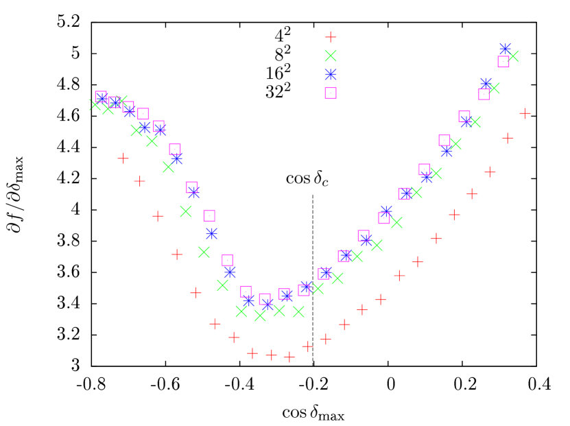
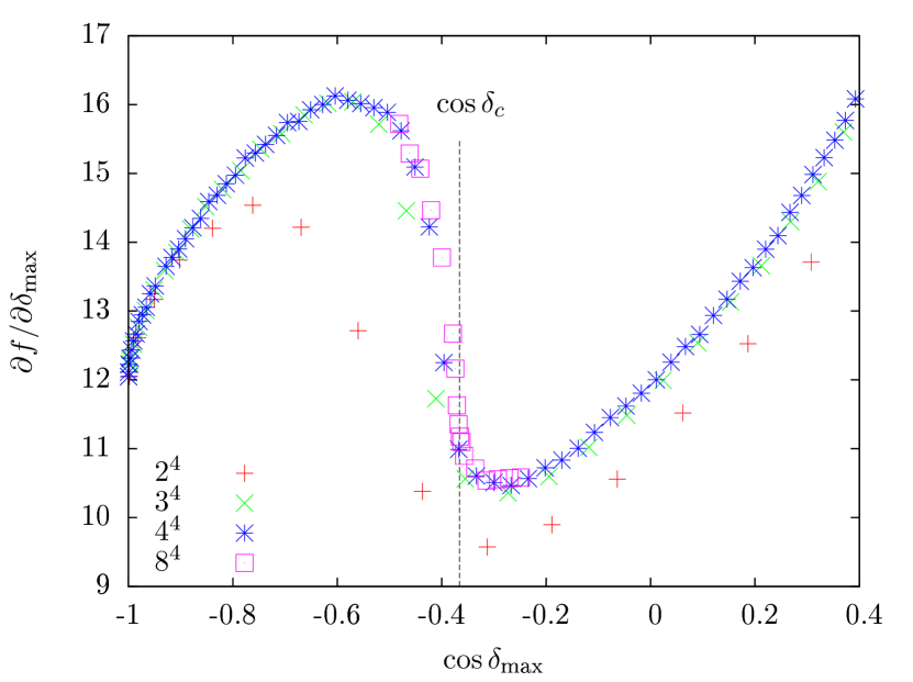
Figure 4: The derivative $\partial f/\partial\delta_{\text{max}}$ of the free energy density $f=-V^{-1}\log Z$ for the $2d$ $XY$-model (upper panel) and the $4d$ $U(1)$ gauge theory (lower panel) as obtained from Monte Carlo simulations with a topological action. There is a clear distinction between the smooth derivative in the $XY$-model which has an infinite order phase transition and the discontinuous behavior, signaling a first order transition, in the $U(1)$ gauge theory. The vertical line marks the critical restriction $\cos\delta_{c}$. In the case of the XY-model it has been taken from Bietenholz et al. (2013) where it was extracted from a fit of the diverging correlation length.

VII Results

Let us now turn to the numerical results. Primarily what we are interested in is the phase structure of the model and the order of the possible deconfinement transition. To this end we have measured the monopole density and the helicity modulus as a function of the restriction $\cos\delta_{\text{max}}$. We compare these results with the corresponding observables obtained with the Wilson action in Figs. 5 and 6: it is obvious that the transition is even weaker than the weak first order transition seen with the Wilson action. We can try to quantify the strength of the transition by fitting the helicity modulus in the confining phase using a simple model of a first order transition Borgs and Kotecky (1992); Vettorazzo and de Forcrand (2004).

$$h(x)=\frac{h_{+}}{1+X^{-1}\exp\left(-V\Delta{}f(x-x_{c})\right)},$$ (16)

where $h_{+}$ is the helicity modulus in the Coulomb phase (which is assumed to be constant), $\Delta{}f$ is the latent heat, $X$ is an anisotropy factor between the two phases and $x$ is the coupling, either $\beta$ or $\cos\delta_{\rm max}$. After taking finite size effects into account the best fit is shown as the lines in Fig. 6. The data is well described by the ansatz and one finds that the fitted value of the latent heat for the Topological action is about half of what it is using the Wilson action, which is consistent with the weaker transition seen in the monopole density.

To further establish that the transition really is first order we show histograms of the monopole density close to the transition for three different volumes in Fig. 7. A double peak structure is formed and enhanced as the volume increases, which is a clear indication that the transition is first order. Also the Monte Carlo history shows clear tunneling events between two metastable states. Together with the discontinuity in the first derivative of the free energy with respect to the cutoff we conclude that the topological action has a first order transition at $\delta_{\text{max}}\approx 1.95$.

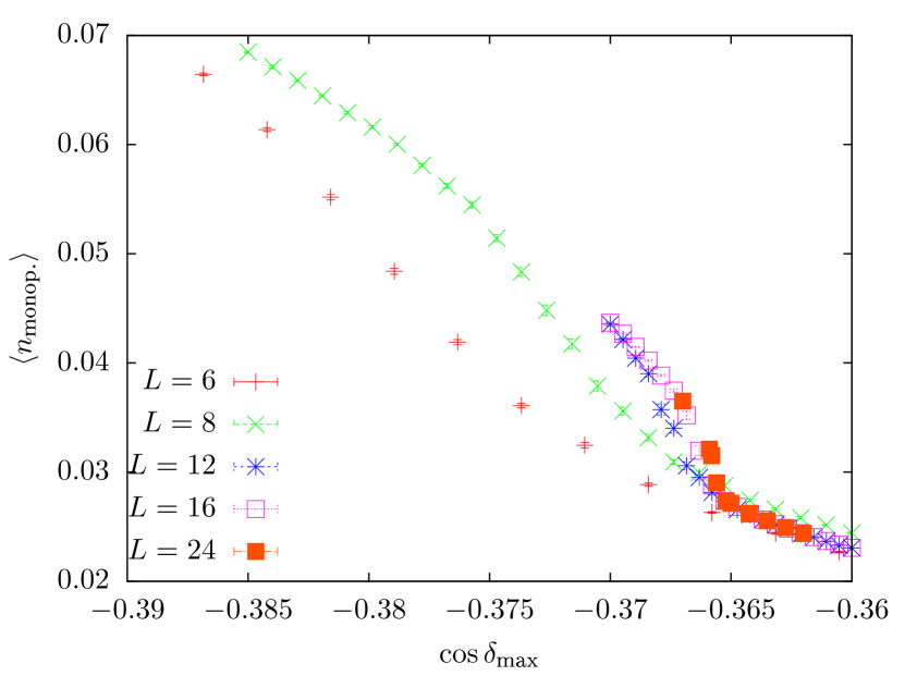
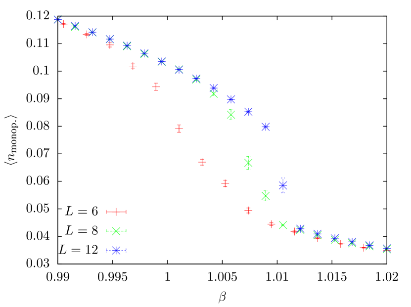
Figure 5: The monopole density $n$ for the topological action (upper panel) and the Wilson action (lower panel). For the Wilson action the first order nature of the transition is rather evident even for a $12^{4}$ lattice whereas for the topological action we have to go to much larger lattices to see a fairly distinct jump.

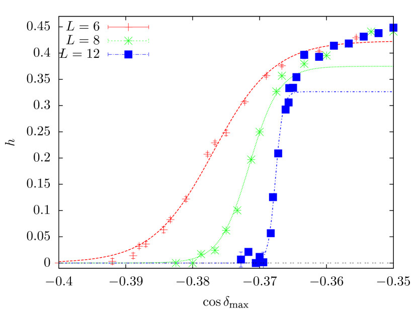
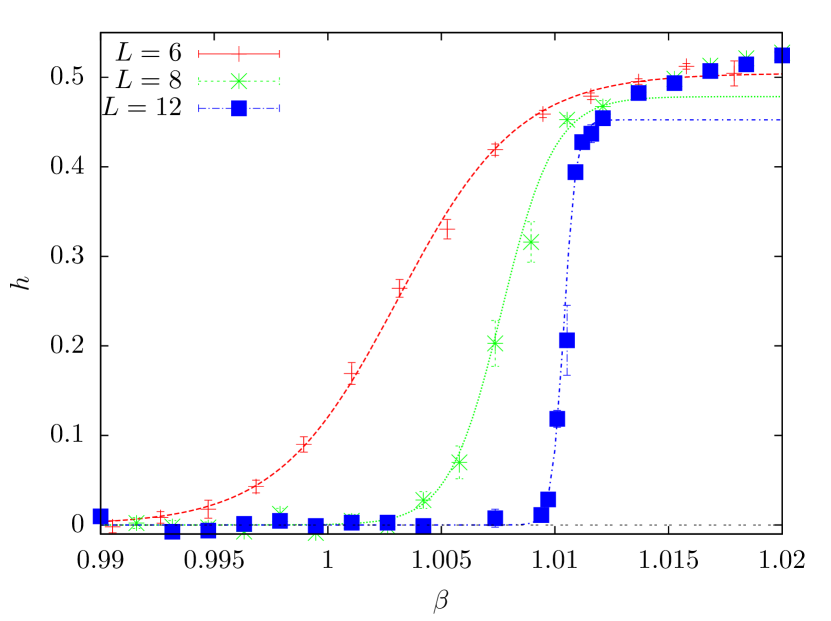
Figure 6: The helicity modulus $h$ for the topological action (upper panel) and the Wilson action (lower panel). The lines are the best fit to eq. (16), which describes the data in the confining phase (the model assumes a constant $h$ in the Coulomb phase) very well for both actions.

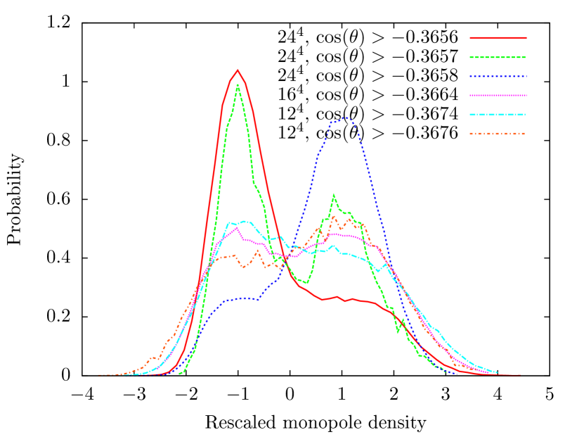
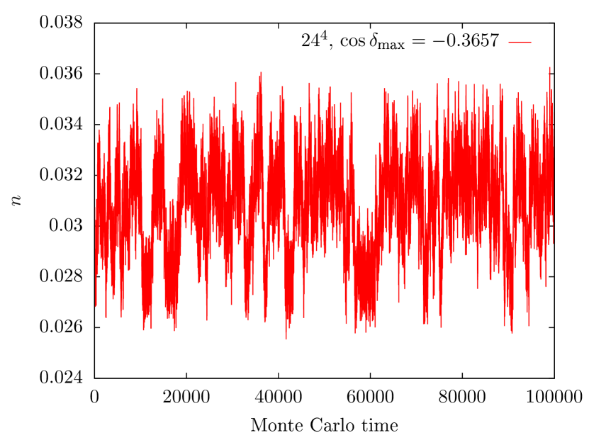
Figure 7: The probability distribution of the monopole density close to the transition for various volumes (upper panel) and the corresponding Monte Carlo history for the $24^{4}$ volume (lower panel). The distributions are rescaled in such a way that one peak is at -1 and the other at +1. That way the separation of the peaks in relation to the widths can be directly compared between different volumes. It is evident that the two peaks become more distinct for larger volumes which indicates a first order transition. Also the obvious tunneling between two different states in the Monte Carlo history backs up this statement.

To determine the characteristics of the two phases we look at how Wilson loops of different sizes behave. Naively, we expect an area law when $\delta_{\text{max}}$ is close to $\pi$ since the interaction between plaquettes will be very weak, as for the Wilson action where $\beta\ll 1$. This can be seen in the left panel of Fig. 1. If the forbidden regions become very narrow then the individual links are hardly influenced by their neighbors and each plaquette angle is more or less uniformly distributed in the interval $[-\delta_{\text{max}},\delta_{\text{max}}]$ which gives an average plaquette trace of $\sin(\delta_{\text{max}})/\delta_{\text{max}}$. For a loop with area $A$, this is raised to the $A$’th power. For restrictions $\delta_{\text{max}}$ close to zero on the other hand, the links are heavily influenced by their neighbors (right panel of Fig. 1) and the total angle of the loop should depend on the perimeter rather than the area. This is demonstrated in Fig. 8 where we show the Creutz ratios

$$\chi(R)=-\log\frac{\left\langle W(R,R)\right\rangle\left\langle W(R-1,R-1)\right\rangle}{\left\langle W(R,R-1)\right\rangle\left\langle W(R-1,R)\right\rangle},$$ (17)

where $W(I,J)$ is a planar, rectangular Wilson loop with sides $I$ and $J$. We have performed the $R\to\infty$ extrapolation under the assumption that the corrections are of the form $e^{-R}$. Note that this is not a precise measurement of the string tension but rather a characterization of the two phases. We have also checked that the magnitude of the Polyakov loop acquires a vacuum expectation value in the low monopole density phase.

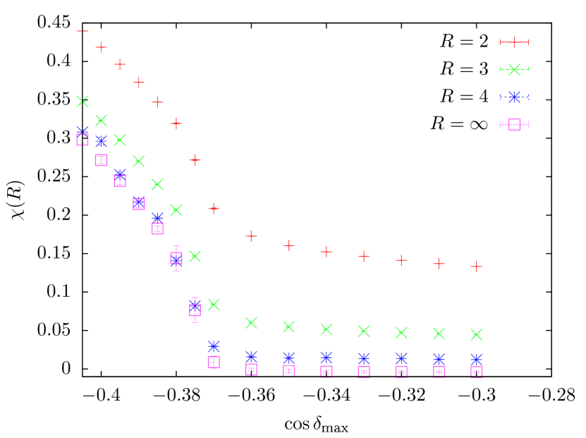
Figure 8: The Creutz ratios $\chi(R)$ given by eq. (17) as well as an $R\to\infty$ extrapolation assuming corrections of the form $e^{-R}$ as a function of the restriction $\cos\delta_{\text{max}}$ obtained on an $8^{4}$ lattice. There is a clear transition between a confining phase with nonzero string tension and a deconfined phase with an perimeter law for the Wilson loops.

Another interesting thing to investigate is how the monopole density depends on the renormalized coupling. The monopole mass is proportional to $\beta_{R}=e_{R}^{-2}$ and the density decreases exponentially with the mass. This is a statement about physics so it gives us a direct way to compare the two actions. In Fig. 9 we show the monopole density as a function of the renormalized coupling and we see a clear exponential decay as expected. For the topological action the decay is significantly faster, which could be interpreted as a reduction in the discretization errors: for a given effective coupling, there are fewer lattice artifacts (monopoles) that disturb the order of the system. For $\delta_{\text{max}}<\pi/3$ the density is even strictly zero and the model is completely insensitive (up to trivial rescalings) to further reduction of $\delta_{\text{max}}$.

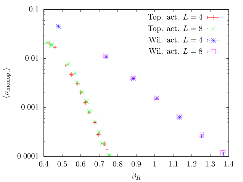
Figure 9: The monopole density in the Coulomb phase as a function of the renormalized coupling $\beta_{R}$, for the topological and the Wilson actions. The different rates of decay could be attributed to different lattice spacings for the two actions.

With a mix of single- and two-link updates we have been able to measure the monopole density down to densities around $10^{-8}$. The exponential dependence on $\cos\delta_{\text{max}}$ persists to $\delta_{\text{max}}\approx 1.69$ after which the density smoothly changes into a power law in $(1/2-\cos\delta_{\text{max}})$ with an exponent which is fitted to be $11.70(6)$ as can be seen in Fig. 10. We tentatively ascribe this change of functional behavior to the approach of a phase transition. A naive argument, which works well in the 2$d$ $XY$-model, leads to a monopole density which is polynomial in the small deviation $(\delta_{\text{max}}-\pi/3)$. The argument is based on convolutions of (near) uniform plaquette or link distributions. To create a single vortex in the spin model close to the threshold $\pi/2$ we need to convolve the link angle distribution four times, which makes the joint distribution $\propto(4\delta_{\text{max}}-\theta)^{3}$ for the cumulative angle $\theta$ around a plaquette. This needs to be evaluated at $\theta=2\pi$ (one vortex) which gives a vortex probability $\propto(\delta_{\text{max}}-\pi/2)^{3}$. Vortices always come in pairs so we expect that the density is proportional to $(\delta_{\text{max}}-\pi/2)^{6}$ which is in good agreement with what we have obtained from Monte Carlo simulations. By a similar argument one would expect a monopole density $\propto(\delta_{\text{max}}-\pi/3)^{20}$ due to six plaquettes in 4 cubes containing a monopole. The deviation in the power law from the predicted $20$ to the observed $\approx 12$ is rather large, but the argument does not take into account that the 4 monopoles are not independent of each other, so it is not so surprising that one finds a smaller exponent.

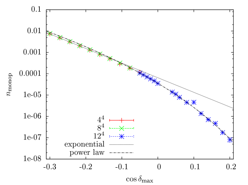
Figure 10: The monopole density for the topological action as a function of the restriction. There seems to be a smooth transition from an exponential decay to a power law at $\cos\delta_{\text{max}}\approx-0.12$.

VIII Conclusions

We have simulated $U(1)$ lattice gauge theory using an unconventional “topological” action. We find that this action describe the same physics as the Wilson action, i.e. there is a confining strong coupling phase where magnetic monopoles condense and Wilson loops follow an area law, separated by a (weak) first order transition from a Coulomb phase with an exponentially suppressed monopole density and a perimeter law for the Wilson loops. We have, in this specific case, not found any concrete advantages which would motivate the choice of this action over the Wilson action although at a given value of the effective coupling in the Coulomb phase there are significantly fewer monopoles (lattice artifacts). This is in line with other known cases where a topological action reduces discretization errors Bietenholz et al. (2013). Perhaps the most interesting approach is to search for optimized combinations of a standard action and constrained fields. An interesting feature of the topological action is the direct access to the free energy itself.

One interesting open question is the nature of the extra transition at $\delta_{\text{max}}=\pi/3$ where there is a non-analyticity in the monopole density as it goes from nonzero to strictly zero. A similar phenomenon occurs at $\delta_{\text{max}}=\pi/2$ for an XY model, and when plaquettes become restricted by the “admissibility condition” in gauge theories. One may argue, however, in the $U(1)$ case at least, that this transition will have no impact on the physics because the monopole density close to the transition is extremely small anyway.

References

- Symanzik (1983) K. Symanzik, Nucl.Phys. B226, 205 (1983).
- Weisz (1983) P. Weisz, Nucl.Phys. B212, 1 (1983).
- Meurice (2002) Y. Meurice, Phys.Rev.Lett. 88, 141601 (2002), arXiv:hep-th/0103134 [hep-th] .
- Michael and Teper (1988) C. Michael and M. Teper, Nucl.Phys. B305, 453 (1988).
- Rufenacht and Wenger (2001) P. Rufenacht and U. Wenger, Nucl.Phys. B616, 163 (2001), arXiv:hep-lat/0108005 [hep-lat] .
- Mack and Pietarinen (1982) G. Mack and E. Pietarinen, Nucl.Phys. B205, 141 (1982).
- Bornyakov et al. (1991) V. Bornyakov, M. Creutz, and V. Mitrjushkin, Phys.Rev. D44, 3918 (1991).
- Fingberg et al. (1995) J. Fingberg, U. M. Heller, and V. Mitrjushkin, Nucl.Phys. B435, 311 (1995), arXiv:hep-lat/9407011 [hep-lat] .
- Luscher (1982) M. Luscher, Commun.Math.Phys. 85, 39 (1982).
- Bietenholz et al. (2010) W. Bietenholz, U. Gerber, M. Pepe, and U.-J. Wiese, JHEP 1012, 020 (2010), arXiv:1009.2146 [hep-lat] .
- Bietenholz et al. (2013) W. Bietenholz, M. Bögli, F. Niedermayer, M. Pepe, F. Rejon-Barrera, et al., JHEP 1303, 141 (2013), arXiv:1212.0579 [hep-lat] .
- DeGrand and Toussaint (1980) T. A. DeGrand and D. Toussaint, Phys.Rev. D22, 2478 (1980).
- Note (1) However, it should also be noted that the monopole is a lattice artifact which disappears in the continuum limit also for the Wilson action.
- Nelson and Kosterlitz (1977) D. R. Nelson and J. Kosterlitz, Phys.Rev.Lett. 39, 1201 (1977).
- Vettorazzo and de Forcrand (2004) M. Vettorazzo and P. de Forcrand, Nucl.Phys. B686, 85 (2004), arXiv:hep-lat/0311006 [hep-lat] .
- Budczies and Zirnbauer (2003) J. Budczies and M. Zirnbauer, (2003), arXiv:math-ph/0305058 [math-ph] .
- Borgs and Kotecky (1992) C. Borgs and R. Kotecky, Phys.Rev.Lett. 68, 1734 (1992).