Viriato: a Fourier-Hermite spectral code for strongly magnetised fluid-kinetic plasma dynamics

Abstract

We report on the algorithms and numerical methods used in Viriato, a novel fluid-kinetic code that solves two distinct sets of equations: (i) the Kinetic Reduced Electron Heating Model (KREHM) equations [Zocco & Schekochihin, Phys. Plasmas 18, 102309 (2011)] (which reduce to the standard Reduced-MHD equations in the appropriate limit) and (ii) the kinetic reduced MHD (KRMHD) equations [Schekochihin et al., Astrophys. J. Suppl. 182:310 (2009)]. Two main applications of these equations are magnetised (Alfvénic) plasma turbulence and magnetic reconnection. Viriato uses operator splitting (Strang or Godunov) to separate the dynamics parallel and perpendicular to the ambient magnetic field (assumed strong). Along the magnetic field, Viriato allows for either a second-order accurate MacCormack method or, for higher accuracy, a spectral-like scheme composed of the combination of a total variation diminishing (TVD) third order Runge-Kutta method for the time derivative with a 7th order upwind scheme for the fluxes. Perpendicular to the field Viriato is pseudo-spectral, and the time integration is performed by means of an iterative predictor-corrector scheme. In addition, a distinctive feature of Viriato is its spectral representation of the parallel velocity-space dependence, achieved by means of a Hermite representation of the perturbed distribution function. A series of linear and nonlinear benchmarks and tests are presented, including a detailed analysis of 2D and 3D Orszag-Tang-type decaying turbulence, both in fluid and kinetic regimes.

url]http://web.ist.utl.pt/nuno.f.loureiro

1 Introduction

Magnetised plasma dynamics lies at the heart of many fascinating phenomena in astro, space and laboratory physics. Turbulence in the solar wind [1] and in the interstellar medium [2], solar [3], stellar [4] and accretion disk flares [5], substorms in the Earth’s magnetosphere [6], and turbulent transport and instabilities in magnetised fusion experiments [7], are just a few examples of remarkable physics problems whose solution is indeed determined by understanding the behaviour of plasmas in a magnetised environment.

In many of these cases, (i) the collision frequency is much lower than the typical frequencies of the physical phenomena of interest (e.g., turbulence, magnetic reconnection) — i.e., the plasmas are weakly collisional; and (ii) the size of the ion Larmor orbit is several orders of magnitude smaller than the size of the system. Weak collisionality implies that on the timescales of interest the plasma cannot be treated as a fluid, and instead a kinetic description that evolves the particles’ distribution functions is required. This is rather unfortunate from the computational point of view, since fully kinetic models live on a six-dimensional phase-space (each particle is characterised by its position and velocity vectors). The strong magnetisation, however, implies that the plasma is highly anisotropic, with very different particle motions along and across the magnetic field direction. This anisotropy can be explored analytically to yield reduced kinetic models, i.e., asymptotic descriptions that reduce the phase-space to only 5D or even 4D. This leads to tremendous computational savings and effectively renders possible calculations that would otherwise not be feasible on today’s supercomputers.

Gyrokinetics [8, 9, 10, 11, 12] is a rigorous description of strongly magnetised, weakly-collisional plasmas. The key idea behind the gyrokinetic formalism is that, because of the strong magnetic (guide) field, the particles’ Larmor gyration frequency is much higher than the frequencies of dynamical interest, and can thus be averaged over. This allows for the reduction of the dimensionality of the system, from 6D (three position and three velocity coordinates) to 5D (three position coordinates, and velocities parallel and perpendicular to the magnetic field) while retaining all the essential physical effects. Gyrokinetics was originally motivated by the attempt to model microinstabilities in magnetic fusion experiments; in this respect it has been rather successful [10, 11]. As recognition of its usefulness, the range of applications of gyrokinetics has broadened in recent years; it is now routinely applied to the study of turbulence in magnetised astrophysical systems [9, 13, 14, 15], and there have also been some studies pioneering its application to the problem of magnetic reconnection [16, 17, 18, 19, 20].

This reduction of the dimensionality of the system allowed by gyrokinetics is extremely advantageous from the numerical point of view. Nonetheless, intrinsically multiscale problems such as kinetic turbulence and reconnection remain formidable computational challenges. Further simplification where possible is therefore desirable.

One possible such simplification of gyrokinetics has recently been proposed by Zocco and Schekochihin [21]: the Kinetic Reduced Electron Heating Model (KREHM), a rigorous asymptotic limit of gyrokinetics valid for plasmas such that

$$\beta_{e}\sim m_{e}/m_{i},$$ (1)

where $\beta_{e}=8\pi n_{0e}T_{0e}/B_{0}^{2}$ is the electron beta, $n_{0e},~{}T_{0e}$ are the background electron density and temperature, respectively, and $B_{0}$ is the background magnetic field. Under this assumption, Ref. [21] shows that it is possible to reduce the plasma dynamics to a 4D phase-space — position and velocity parallel to the magnetic field — while retaining key physics such as phase-mixing and electron Landau damping, ion finite Larmor radius effects, electron inertia, electron collisions and Ohmic resistivity. This is a very significant simplification of the full kinetic description, which renders possible truly multiscale kinetic simulations. In particular, because no ad hoc fluid closure is employed, KREHM can be used for detailed studies of energy conversion and dissipation in kinetic turbulence and reconnection, including electron heating via phase-mixing and Landau damping.

If taken literally, the ordering imposed by equation (1) is somewhat restrictive, and obviously excludes many plasmas of interest. Examples of plasmas where it may hold are some regions of the solar corona [22, 23], the LArge Plasma Device (LAPD) experiment at UCLA [24], and edge regions in some tokamaks [25]. However, one may legitimately expect that the plasma behaviour captured by KREHM will qualitatively hold beyond its rigorous limits of applicability, as is so often the case with many other simplified plasma models (MHD being a notorious example of a description known to work rather well far outside its strict limits of validity). Hints that this may indeed be the case are offered in section 7.3, where a direct comparison of KREHM with a (non-reduced) gyrokinetic model for the linear collisionless tearing mode problem yields very good agreement at values of $\beta_{e}$ significantly larger than $m_{e}/m_{i}$.

This paper reports on the numerical methods and algorithms used in Viriato, the first numerical code to solve this particular set of equations. An extensive series of tests and benchmarks is also presented. Considerable attention is devoted to Orszag-Tang-type decaying turbulence, both in the fluid and kinetic regimes. The reader interested in the application of this code and physics model to the problem of magnetic reconnection is referred to [26], where the importance of electron heating via Landau damping in reconnection is demonstrated for the first time.

A second set of equations solved by Viriato are the kinetic reduced MHD (KRMHD) equations [14], which describe the evolution of compressible fluctuations (density and parallel magnetic field) in the regime $k_{\perp}\rho_{i}\ll 1$ ($k_{\perp}$ being the wave number perpendicular to the guide-field of a typical perturbation, and $\rho_{i}$ the ion Larmor radius.) These equations are structurally identical to those of KREHM, so their numerical implementation in Viriato is straightforward. We also note that KREHM reduces to the standard Reduced-MHD (RMHD) set of equations [27, 28] in the appropriate limit (i.e., when the wave length of the fluctuations is much larger than all the kinetic scales). Thus, Viriato can also be used as a RMHD code (in either 2D or 3D slab geometry). Finally, we remark that under an isothermal closure for the electrons, KREHM reduces to the simple two-field gyrofluid model treated in Refs. [29, 30] (which is a limit of the more complete models of Snyder et al. [31] and of Schep et al. [32]).

This paper is organized as follows. Section 2 presents the different sets of equations integrated by Viriato. The kinetic equations are solved by means of a Hermite expansion, which requires some form of closure (or truncation). This is discussed in section 3, where an asymptotically exact nonlinear closure for the Hermite-moment hierarchy is derived. Section 4 presents the energy evolution equation for the closed KREHM model; and the normalizations that we adopt are laid out in section 5. Section 6 deals with the numerical discretization of the equations, including in section 6.2 a discussion of the implementation of a spectral-like scheme for the advection in the direction along the guide-field: a combination of an optimal third order total variation diminishing (TVD) Runge Kutta [33] for the time derivative with a seventh-order upwind scheme for the fluxes [34]. A series of linear and nonlinear benchmarks of the code are presented in section 7, with emphasis on Orszag-Tang-type decaying turbulence test cases. Finally, the main points and results of this paper are summarised in  section 9. Also included for reference in Appendix A is the recently proposed modification of the KREHM model to allow for background electron temperature gradients [35].

2 Sets of Equations solved by Viriato

Viriato solves two distinct sets of equations: (i) the Kinetic Reduced Electron Heating Model (KREHM) equations [21] and (ii) the Kinetic Reduced MHD (KRMHD) equations [14]. These models are briefly discussed below; we refer the interested reader to the original references for a detailed derivation of the equations of each model.

2.1 The Kinetic Reduced Electron Heating Model (KREHM)

The Kinetic Reduced Electron Heating Model (KREHM) derived in Ref. [21] is a rigorous asymptotic reduction of standard gyrokinetics [8, 9, 10, 11, 12] applicable to plasmas that verify equation (1). In the slab geometry that we adopt, the background magnetic field (the guide-field) is assumed to be straight and uniform, $\bm{B}_{0}=B_{0}\bm{e}_{z}$. The perturbed electron distribution function, to lowest order in $\sqrt{m_{e}/m_{i}}\sim\sqrt{\beta}_{e}$, and in the gyrokinetic expansion, is defined as

$$\delta f_{e}=g_{e}+(\delta n_{e}/n_{0e}+2v_{\parallel}u_{\parallel e}/v_{{\rm th}e}^{2})F_{0e},$$ (2)

where $F_{0e}$ is the equilibrium Maxwellian, $v_{{\rm th}e}=\sqrt{2T_{0e}/m_{e}}$ is the electron thermal speed, $v_{\parallel}$ is the velocity coordinate parallel to the guide-field direction, $\delta n_{e}$ is the electron density perturbation (the zeroth moment of $\delta f_{e}$), and

$$u_{\parallel e}=-j_{\parallel}/n_{0e}e=(e/cm_{e})d_{e}^{2}\nabla_{\perp}^{2}A_{\parallel}$$ (3)

is the parallel electron flow (the first moment of $\delta f_{e}$). In this expression, $j_{\parallel}$ is the parallel current and $A_{\parallel}$ is the parallel component of the vector potential (note that, in this model, the parallel ion flow is zero to the order that is kept in the expansion); and $d_{e}=c/\omega_{pe}$ is the electron skin depth, where $\omega_{pe}=\sqrt{4\pi n_{0e}e^{2}/m_{e}}$ is the electron plasma frequency. All moments of $\delta f_{e}$ higher than $\delta n_{e}$ and $u_{\parallel e}$ are contained in the “reduced” electron distribution function $g_{e}$, e.g., parallel temperature fluctuations are given by

$$\frac{\delta T_{\parallel e}}{T_{0e}}=\frac{1}{n_{0e}}\int d^{3}{\bm{v}}~{}\frac{2v_{\parallel}^{2}}{v_{{\rm th}e}^{2}}~{}g_{e}.$$ (4)

For notational simplicity, let us introduce the following usual definitions:

$$\frac{d}{dt} = \frac{\partial}{\partial t}+\frac{c}{B_{0}}\left[\varphi,\dots\right],$$ (5)

$$\hat{\bm{b}}\cdot\nabla = \frac{\partial}{\partial z}-\frac{1}{B_{0}}\left[A_{\parallel},\dots\right],$$ (6)

where $\varphi$ is the electrostatic potential and $\left[\dots,\dots\right]$ denotes the Poisson bracket. The KREHM equations are [21]:

$$\frac{1}{n_{0e}}\frac{d\delta n_{e}}{dt}=-\hat{\bm{b}}\cdot\nabla\frac{e}{cm_{e}}d_{e}^{2}\nabla^{2}_{\perp}A_{\parallel},$$ (7)

$$\frac{d}{dt}\left(A_{\parallel}-d_{e}^{2}\nabla^{2}_{\perp}A_{\parallel}\right)=\eta\nabla^{2}_{\perp}A_{\parallel}-c\frac{\partial\varphi}{\partial z}+\frac{cT_{0e}}{e}\hat{\bm{b}}\cdot\nabla\left(\frac{\delta n_{e}}{n_{0e}}+\frac{\delta T_{\parallel e}}{T_{0e}}\right),$$ (8)

$$\frac{dg_{e}}{dt}+v_{\parallel}\hat{\bm{b}}\cdot\nabla\left(g_{e}-\frac{\delta T_{\parallel e}}{T_{0e}}F_{0e}\right)=C[g_{e}]+\left(1-\frac{2v_{\parallel}^{2}}{v_{{\rm th}e}^{2}}\right)F_{0e}\hat{\bm{b}}\cdot\nabla\frac{e}{cm_{e}}d_{e}^{2}\nabla^{2}_{\perp}A_{\parallel}.$$ (9)

Here, $\eta$ is the Ohmic diffusivity and $C[g_{e}]$ is the collision operator.

The perturbed electron density and the electrostatic potential are related via the gyrokinetic Poisson law [36]:

$$\frac{\delta n_{e}}{n_{0e}}=\frac{Z}{\tau}\left(\hat{\Gamma}_{0}-1\right)\frac{e\varphi}{T_{0e}},$$ (10)

where $\tau=T_{0i}/T_{0e}$ and $\hat{\Gamma}_{0}$ denotes the inverse Fourier transform of $\Gamma_{0}(\alpha)=I_{0}(\alpha)e^{-\alpha}$, with $I_{0}$ the modified Bessel function and $\alpha=k_{\perp}^{2}\rho_{i}^{2}/2$ ($\rho_{i}=v_{{\rm th}i}/\Omega_{i}$ is the ion Larmor radius, with $v_{{\rm th}i}=\sqrt{2T_{0i}/m_{i}}$ the ion thermal velocity and $\Omega_{i}=ZeB_{0}/m_{i}c$ the ion gyrofrequency).

Equation (9) is a kinetic equation for the reduced electron distribution function $g_{e}(x,y,z,v_{\parallel},v_{\perp},t)$. An important observation is that it does not contain an explicit dependence on $v_{\perp}$. If such a dependence is not introduced by the collision operator $C[g_{e}]$, then $v_{\perp}$ can be integrated out, and the reduced electron distribution function becomes effectively 4D only, $g_{e}=g_{e}(x,y,z,v_{\parallel})$.

2.1.1 Hermite expansion

The use of a Hermite polynomial expansion of the distribution function is a well-known technique to simplify the numerical solution of kinetic equations such as (9) [37, 38, 39, 40, 41, 42, 43] — see [41] in particular for an insightful discussion of this approach. A very convenient aspect of the Hermite formulation is that it enables a spectral representation of velocity space, a highly-desirable property when the available resolution is limited (as is almost invariably the case). It is worth pointing out, furthermore, that the advantages of the Hermite representation transcend the numerical aspects, as it often enables one to make analytical headway in problems that are otherwise too complex: see, e.g., Refs. [21, 44, 35, 45].

Perhaps for both these reasons, Hermite formulations have gathered considerable interest recently; we refer the reader to Ref. [46] for a very comprehensive overview of recent and past work on the subject.

The Hermite expansion of $g_{e}$ is defined by

$$g_{e}(x,y,z,v_{\parallel},t)=\sum_{m=2}^{\infty}\frac{1}{\sqrt{2^{m}m!}}H_{m}\left(\frac{v_{\parallel}}{v_{{\rm th}e}}\right)g_{m}(x,y,z,t)F_{0e}(v_{\parallel}),$$ (11)

where $H_{m}$ denotes the Hermite polynomial of order $m$ and $g_{m}$ is its coefficient. Note that $g_{0}=g_{1}=0$ because $\delta n_{e}$ and $u_{\parallel e}$ have been explicitly separated in the decomposition of $\delta f_{e}$ given in equation (2).

Introducing this expansion into equation (9), and choosing a modified Lenard-Bernstein collision operator [21], yields a set of coupled, fluid-like equations for the coefficients of the Hermite polynomials:

$$\frac{dg_{m}}{dt}+v_{{\rm th}e}\hat{\bm{b}}\cdot\nabla\left(\sqrt{\frac{m+1}{2}}g_{m+1}+\sqrt{\frac{m}{2}}g_{m-1}-\delta_{m,1}g_{2}\right)=$$

$$-\sqrt{2}\delta_{m,2}\hat{\bm{b}}\cdot\nabla\frac{e}{cm_{e}}d_{e}^{2}\nabla^{2}_{\perp}A_{\parallel}-\nu_{ei}\left(mg_{m}-2\delta_{m,2}g_{2}\right),$$ (12)

where $\delta_{m,2}$ is a Kronecker delta and $\nu_{ei}$ is the electron-ion collision frequency. In addition, this choice for $C[g_{e}]$ defines the resistive diffusivity:

$$\eta\equiv\nu_{ei}d_{e}^{2}.$$ (13)

In the Hermite formulation, $m$ is the velocity-space equivalent of $k$ in the usual Fourier representation of position space. Thus, for example, the formation of fine scale structures in velocity space (as arises from phase-mixing) can be conveniently thought of as a transfer of energy to high $m$’s, much in the same way as the formation of fine scales in real space leads to energy being transferred to high wave numbers $k$ in the usual Fourier representation. On the other hand, the Hermite representation introduces a closure problem, in that the equation for $g_{m}$ couples to the higher order moment $g_{m+1}$. We shall see in section 3, however, that a rigorous, nonlinear closure can be obtained.

2.1.2 Reduced MHD limit

The well known reduced MHD (RMHD) equations [27, 28] can be obtained from equations (7–10) by taking the collisional limit $\nu_{ei}\gg\omega$, $k_{\perp}\ll\left(\rho_{i}^{-1},\rho_{s}^{-1},d_{e}^{-1}\right)$, where $\omega$ and $k_{\perp}$ represent the typical frequencies and perpendicular wave numbers of the fluctuations, and $\rho_{s}=\rho_{i}/{\sqrt{2\tau}}$ is the ion sound Larmor radius.

In this limit, the isothermal approximation, $\delta T_{\parallel e}=0$, applies, and thus equation (9) decouples from equations (7–8). For $k_{\perp}\rho_{i}\ll 1$, equation (10) becomes

$$\frac{\delta n_{e}}{n_{0e}}=\frac{1}{\Omega_{i}}\nabla^{2}_{\perp}\Phi,$$ (14)

where we have defined $\Phi\equiv c\varphi/B_{0}$ to make contact with the standard terminology. Further defining $A_{\parallel}\equiv-\sqrt{4\pi n_{0}m_{i}}\Psi$, we obtain:

$$\frac{\partial}{\partial t}\nabla^{2}_{\perp}\Phi+\left[\Phi,\nabla^{2}_{\perp}\Phi\right] = v_{A}\frac{\partial}{\partial z}\nabla^{2}_{\perp}\Psi+\left[\Psi,\nabla^{2}_{\perp}\Psi\right],$$ (15)

$$\frac{\partial\Psi}{\partial t}+\left[\Phi,\Psi\right] = \eta\nabla^{2}_{\perp}\Psi+v_{A}\frac{\partial\Phi}{\partial z},$$ (16)

where $v_{A}$ is the Alfvén speed based on the guide-field, $v_{A}=B_{0}/\sqrt{4\pi n_{0}m_{i}}$.

2.2 Kinetic Reduced Magnetohydrodynamics (KRMHD)

A different set of equations solved by Viriato  is the Kinetic Reduced Magnetohydrodynamics (KRMHD) model, derived by expanding the gyrokinetic equation in terms of the small parameter $k_{\perp}\rho_{i}$ [14]—in this sense, it is the long wavelength limit of gyrokinetics. In this limit, the Alfvénic component of the turbulent fluctuations decouples from the compressive component. The dynamics of the system are completely determined by the Alfvénic fluctuations, which are governed by the reduced MHD equations (15–16). The compressive fluctuations, on the other hand, evolve according to a kinetic equation:

$$\frac{dg}{dt}+v_{\parallel}\hat{\bm{b}}\cdot\nabla g = \frac{v_{\parallel}F_{0}}{\Lambda}\hat{\bm{b}}\cdot\nabla\int dv_{\parallel}g,$$ (17)

where $g$ is related to the perturbed ion distribution function [see equation (183) of Schekochihin et al. [14]] and $F_{0}=\exp(-v_{\parallel}^{2}/v_{{\rm th}i}^{2})/\sqrt{\pi v_{{\rm th}i}}$ is a one dimensional Maxwellian. The parameter $\Lambda$ is a linear combination of the physical parameters ion-to-electron temperature ratio, plasma beta, and the ion charge [see equation (182) of Schekochihin et al. [14]].

The structure of Eq. (17) is mathematically similar to that of Eq. (9), the main difference being that this kinetic equation is decoupled from the Alfvénic fluctuations, unlike its KREHM counterpart.

Similar to section 2.1.1, one obtains the following set of equations by expanding Eq. (17) in terms of Hermite polynomials:

$$\frac{dg_{0}}{dt}+v_{{\rm th}i}\nabla_{\parallel}\frac{g_{1}}{\sqrt{2}}=0,$$ (18)

$$\frac{dg_{1}}{dt}+v_{{\rm th}i}\nabla_{\parallel}\left(g_{2}+\frac{\left(1-1/\Lambda\right)}{\sqrt{2}}\,g_{0}\right)=0,$$ (19)

$$\frac{dg_{m}}{dt}+v_{{\rm th}i}\nabla_{\parallel}\left(\sqrt{\frac{m+1}{2}}\,g_{m+1}+\sqrt{\frac{m}{2}}\,g_{m-1}\right)$$

$$=C[g_{m}],\quad m\geq 2.$$ (20)

Notice that, unlike Eq. (2.1.1), equations (18–2.2) begin at $m=0$. Additionally, since the term on the right hand side of equation (17) is proportional to the first Hermite polynomial, the parameter $\Lambda$ makes an appearance only in the equation for $g_{1}$.

3 Hermite closure

The Hermite expansion transforms the original electron drift-kinetic equation, (9), into an infinite, coupled set of fluid-like equations, (2.1.1) [or, similarly for KRHMD, equation (17) into equations (18–2.2)]. Formally, the two representations are exactly equivalent, i.e., no information is lost by introducing the Hermite representation. However, the numerical implementation of equations (2.1.1) obviously requires some form of truncation, i.e., given a certain number of Hermite moments, $M$, it is necessary to specify some prescription for $g_{M+1}$. In other words, as in the derivation of any fluid set of equations, the Hermite expansion introduces a closure problem. Attempts to solve this problem have varied, from simply setting $g_{M+1}=0$ (e.g., [37, 41, 47, 46]), to polynomial closures in which $g_{M+1}$ is extrapolated from a number of previous moments [40, 47]. Particularly noteworthy is the approach followed by Hammett and co-workers [48, 41, 49, 42, 50] where closures have been carefully designed to rigorously capture the linear Landau damping rates (as well as gyro-radius effects and dominant nonlinearities).

In the system of equations under consideration here, it turns out that an asymptotically exact closure can be obtained in the large $M$ limit. Let us consider that the collision frequency is small but finite. Then, there will be a range of $m$’s for which the collisional term is negligible — one may think of this as the $m$ inertial range: energy is injected into low $m$’s via the coupling with Ohm’s law, and cascades (phase-mixes) to higher $m$’s. However, as $m$ increases, a dissipation range is encountered, when the collisional term in equation (2.1.1) [or in equation (2.2)] is no longer subdominant with respect to the other terms. Roughly speaking, in the dissipation range, energy arrives at $g_{m}$ from $g_{m-1}$ and is mostly dissipated there; only an exponentially smaller fraction is passed on to $g_{m+1}$. One thus expects that $g_{m+1}/g_{m}\ll 1$ in the dissipation range, by definition. The implication of this is that, for $m=M$ in the dissipation range, the dominant balance in the equation for $g_{M+1}$ must be

$$v_{{\rm th}e}\hat{\bm{b}}\cdot\nabla\sqrt{\frac{M+1}{2}}g_{M}\approx-\nu_{ei}(M+1)g_{M+1}.$$ (21)

Solving this equation for $g_{M+1}$ yields the sought closure [26, 35]. The equation for $g_{M}$ therefore becomes:

$$\frac{dg_{M}}{dt}-\kappa_{\parallel e}\hat{\bm{b}}\cdot\nabla\left(\hat{\bm{b}}\cdot\nabla g_{M}\right)+v_{{\rm th}e}\hat{\bm{b}}\cdot\nabla\sqrt{\frac{M}{2}}g_{M-1}=-\nu_{ei}Mg_{M},$$ (22)

where $\kappa_{\parallel e}\equiv v_{{\rm th}e}^{2}/2\nu_{ei}$ is the parallel (Spitzer) thermal diffusivity. It is easy to see how the exact same reasoning leads to the equivalent closure for equation (2.2).

It can be useful to have an a priori estimate of the value of $M$ required to formally justify the asymptotic closure, for a given collision frequency. One such linear estimate is provided in Ref. [21]: if the Hermite spectrum is in steady-state, then the collisional cutoff, $m=m_{c}$, can be shown to occur at:

$$m_{c}=\left(\frac{3}{2\sqrt{2}}\frac{|k_{\parallel}|v_{{\rm th}e}}{\nu_{ei}}\right)^{2/3}.$$ (23)

Thus, we expect the Hermite closure, equation (21), to be valid if $M\gg m_{c}$.

The numerical implementation of equation (22) introduces some difficulties and will be discussed in section 6.3.

3.1 Hypercollisions

Since our primary interest lies in weakly collisional plasmas, one finds that $m_{c}\gg 1$. For example, a simple estimate using standard parameters for the solar corona suggests $m_{c}\approx 10^{4}$; certain experiments on JET [25] suggest $m_{c}\approx 180$ in the edge region, considerably smaller than for the solar corona, but still quite large. Further noticing that such cases are invariably tied to a broad range of spatial scales, thereby also requiring high spatial resolutions, renders obvious the impracticability of such computations: not only must one solve a very large set of nonlinear, coupled PDE’s, as also the stiffness increases, due to the coefficients proportional to $\sqrt{m}$. One possibility of avoiding this problem is to artificially enhance the value of the collision frequency. Note however that $m_{c}\sim\nu_{ei}^{-2/3}$, i.e., a relatively weak scaling, implying that cutting the number of necessary $m$’s down to computationally manageable sizes would require drastic increases in the collision frequency. To make matters worse, the collision operator scales only linearly with $m$, implying that in fact one needs to retain $m\gg m_{c}$ to adequately capture the dissipation range and validate the closure.

One way to circumvent these difficulties is to make use of a ‘hyper-collision’ operator, i.e., add a term of the form $-m^{h}\nu_{H}g_{m}$ to the RHS of equation (2.1.1). Here, $h$ is the order of the hyper-diffusion operator (a typical value would be $h=6$) and $\nu_{H}$ is a numerically-based coefficient defined such that energy arriving at $m=M$ can be dissipated in one timestep:

$$\frac{\partial g_{M}}{\partial t}\sim M^{h}\nu_{H}g_{M}.$$ (24)

Thus, in practice, one may simply set [51, 26]:

$$\nu_{H}=1/(\Delta tM^{h}).$$ (25)

It is worth remarking that if it is possible to choose a value of $M$ that is very deep into the dissipation range, then presumably the issue of which closure to implement becomes less sensitive, and it may be justified to simply set $g_{M+1}=0$. Indeed, we have performed simulations with both closures and observed no differences (not reported in this paper).

Finally, we point out that in alternative to a hyper-collision operator one may use a spectral filter (in $m$-space), such as the one of Hou and Li [52], as proposed by Parker and Dellar [46] (see also section 6.1.1 for a discussion of this filter in Fourier space).

4 Energy

In the absence of collisions, equations (7–9) conserve a quadratic invariant usually referred to as free energy [14]. This quantity can be defined as $W=W_{\rm fluid}+H_{e}$, where [21]

$$W_{\rm fluid}=\sum_{\bm{k}}\left[1+\frac{1}{\tau}(1-\Gamma_{0})\right]\frac{1}{\tau}(1-\Gamma_{0})\frac{e^{2}n_{0e}|\varphi_{\bm{k}}|^{2}}{2T_{0e}}+\int\frac{d^{3}{\bm{r}}}{V}\frac{|\nabla_{\perp}A_{\parallel}|^{2}+d_{e}^{2}|\nabla^{2}_{\perp}A_{\parallel}|^{2}}{8\pi}$$ (26)

is the “fluid” (electromagnetic) part of the free energy, and

$$H_{e}=\int\frac{d^{3}{\bm{r}}}{V}\int d^{3}{\bm{v}}\frac{T_{0e}g_{e}^{2}}{2F_{0e}}$$ (27)

is the electron free energy (i.e., the free energy associated with the reduced electron distribution function $g_{e}$).

Upon introducing the Hermite expansion of $g_{e}$, equation (11), and allowing for finite collisions (modelled by the Lenard-Bernstein collision operator), one finds that $W$ evolves according to the following equation [21]:

$$\frac{d}{dt}W_{\rm fluid}+\frac{d}{dt}\int\frac{d^{3}{\bm{r}}}{V}\frac{n_{0e}T_{0e}}{2}\sum_{m=2}^{\infty}g_{m}^{2}=-n_{0e}T_{0e}\nu_{ei}\int\frac{d^{3}{\bm{r}}}{V}\sum_{m=3}^{\infty}mg_{m}^{2}-\frac{4\pi}{c^{2}}\eta\int\frac{d^{3}{\bm{r}}}{V}j_{\parallel}^{2}.$$ (28)

The above equation is exact. However, as discussed in section 3, the numerical implementation of the Hermite expansion requires that only a finite number of Hermite polynomials are kept, and some form of closure to the expansion is required. If we adopt the closure described by equation (21), and truncate the expansion at $m=M$, equation (28) adopts the truncated form:

$$\frac{d}{dt}W_{\rm fluid}+\frac{d}{dt}\int\frac{d^{3}{\bm{r}}}{V}\frac{n_{0e}T_{0e}}{2}\sum_{m=2}^{M}g_{m}^{2}=$$

$$-n_{0e}T_{0e}\nu_{ei}\int\frac{d^{3}{\bm{r}}}{V}\sum_{m=3}^{M}mg_{m}^{2}-n_{0e}T_{0e}\kappa_{e}\int\frac{d^{3}{\bm{r}}}{V}\left(\hat{\bm{b}}\cdot\nabla g_{M}\right)^{2}-\frac{4\pi}{c^{2}}\eta\int\frac{d^{3}{\bm{r}}}{V}j_{\parallel}^{2},$$

where the second term on the RHS is due to the specific closure that we have used (and would vanish if, for example, we instead use the simpler closure $g_{M+1}=0$.)

The same arguments that were invoked to motivate the Hermite closure in section 3 apply here to justify the asymptotic equivalence of the full form of the energy balance, equation (28) and its truncated version, equation (4) — that is, as long as $M$ is as large as required for $g_{M}$ to lie in the collisional (i.e., $m$-) dissipation range, one expects the terms neglected in going from equation (28) to equation (4) to be exponentially small.

The corresponding equation for KRMHD is equation (4.7) of Ref. [44]. The closure that we propose in  section 3 can be implemented in this set of equations in a similar way, and it is straightforward to obtain the KRMHD counterpart of equation (4).

5 Normalizations

The normalizations that we adopt for the KREHM set of equations (7,8,10,2.1.1) are:

• Length scales:

  $$(\hat{x},\hat{y})=(x,y)/L_{\perp};\quad\hat{z}=z/L_{\parallel},$$ (30)

  where $L_{\perp},~{}L_{\parallel}$ are, respectively, the perpendicular and parallel (to the guide-field) reference length-scales.

• Times:

  $$\hat{t}=t/\tau_{A},$$ (31)

  where $\tau_{A}=L_{\parallel}/v_{A}$ is the parallel Alfvén time.

• Fields:

  $$(\hat{n}_{e},\hat{g}_{m}) = \tau_{A}\Omega_{i}\left(\frac{\delta n_{e}}{n_{0e}},g_{m}\right),$$ (32)

  $$\hat{\varphi} = \frac{c}{B_{0}}\frac{\tau_{A}}{L_{\perp}^{2}}\varphi,$$ (33)

  $$\hat{A}_{\parallel} = \frac{L_{\parallel}}{L_{\perp}}\frac{A_{\parallel}}{L_{\perp}B_{0}}.$$ (34)

Under these normalizations, equations (7), (8) and (2.1.1) become:

$$\frac{dn_{e}}{dt}=\left[A_{\parallel},\nabla^{2}_{\perp}A_{\parallel}\right]-\frac{\partial}{\partial z}\nabla^{2}_{\perp}A_{\parallel},$$ (35)

$$\frac{d}{dt}\left(A_{\parallel}-d_{e}^{2}\nabla^{2}_{\perp}A_{\parallel}\right)=\eta\nabla^{2}_{\perp}A_{\parallel}+\rho_{s}^{2}\left[n_{e}+\sqrt{2}g_{2},A_{\parallel}\right]$$

$$\qquad\qquad-\frac{\partial\varphi}{\partial z}+\rho_{s}^{2}\frac{\partial}{\partial z}\left(n_{e}+\sqrt{2}g_{2}\right),$$ (36)

$$\frac{dg_{2}}{dt}=\sqrt{3}\frac{\rho_{s}}{d_{e}}\left\{\left[A_{\parallel},g_{3}\right]-\frac{\partial g_{3}}{\partial z}\right\}+\sqrt{2}\left\{\left[A_{\parallel},\nabla^{2}_{\perp}A_{\parallel}\right]-\frac{\partial}{\partial z}\nabla^{2}_{\perp}A_{\parallel}\right\},$$ (37)

$$\frac{dg_{m}}{dt}=\sqrt{m+1}\frac{\rho_{s}}{d_{e}}\left\{\left[A_{\parallel},g_{m+1}\right]-\frac{\partial g_{m+1}}{\partial z}\right\}+\sqrt{m}\frac{\rho_{s}}{d_{e}}\left\{\left[A_{\parallel},g_{m-1}\right]-\frac{\partial g_{m-1}}{\partial z}\right\}$$

$$\qquad\qquad-m\nu_{ei}g_{m},\quad m>2.$$ (38)

where now

$$\frac{d}{dt}=\frac{\partial}{\partial t}+\left[\varphi,\dots\right].$$ (39)

The normalized form of the quasi-neutrality equation (10) is

$$n_{e}=\frac{2}{\rho_{i}^{2}}\left[\hat{\Gamma}_{0}(\alpha)-1\right]\varphi.$$ (40)

It can immediately be seen that neglecting the $g^{\prime}s$ reduces the above set of equations to the simpler two-field gyrofluid model treated in [30].

For the KRMHD set of equations (18–2.2) the normalisation of space and time are as above, upon which the only modification is the conversion of the prefactor $v_{{\rm th}i}$ into $\sqrt{\beta_{i}}$, where $\beta_{i}=8\pi n_{0i}T_{0i}/B_{0}^{2}$ is the ion plasma beta. The normalisation of the Hermite moments $g_{m}$ is arbitrary since those equations are linear in $g_{m}$.

6 Numerical discretization

The RHS of equations (35–5) is conveniently separated into operators acting either in the direction perpendicular ($x,~{}y$) or parallel ($z$) to the guide field. This suggests that an efficient way of integrating those equations is to use operator splitting techniques such as to individually handle each class (perpendicular or parallel) of operators. Viriato allows for both Godunov [53] or Strang splitting [54]. Although Godunov splitting is formally only 1st-order accurate, direct comparisons of both splitting schemes performed by us (not reported here) yield undistinguishable results. Thus, by default, Viriato employs Godunov splitting (as it is computationally cheaper); all results reported in section 7 are obtained with this option.

We now detail the algorithms employed for the perpendicular and parallel steps.

6.1 Perpendicular direction

The numerical discretisation of equations (35–5) is the straightforward generalisation of that derived in [30]. For presentational simplicity, let us denote the nonlinear terms (i.e., the Poisson brackets) in equations (35–5) by generalised operators, such that we have:

$$\frac{\partial n_{e}}{\partial t} = \mathcal{N}(n_{e},A_{\parallel}),$$ (41)

$$(1+k_{\perp}^{2}d_{e}^{2})\frac{\partial A_{\parallel}}{\partial t} = \mathcal{A}(n_{e},A_{\parallel},g_{2})-\eta k_{\perp}^{2}(A_{\parallel}-A_{\parallel,eq}),$$ (42)

$$\frac{\partial g_{2}}{\partial t} = \mathcal{G}_{2}(n_{e},A_{\parallel},g_{2},g_{3}),$$ (43)

$$\frac{\partial g_{m}}{\partial t} = \mathcal{G}_{m}(n_{e},A_{\parallel},g_{m-1},g_{m},g_{m+1})-m\nu_{ei}g_{m}.$$ (44)

Then, the integration scheme is as follows. First we take a predictor step:

$$n_{e}^{n+1,*} = n_{e}^{n}+\Delta t\mathcal{N}(n_{e}^{n},A_{\parallel}^{n}),$$ (45)

$$A_{\parallel}^{n+1,*} = e^{-D_{\eta}\Delta t}A_{\parallel}^{n}+\left(1-e^{-D_{\eta}\Delta t}\right)A_{\parallel,eq}+$$ (46)

$$\frac{\Delta t}{2}\frac{1+e^{-D_{\eta}\Delta t}}{1+k_{\perp}^{2}d_{e}^{2}}\mathcal{A}(n_{e}^{n},A_{\parallel}^{n},g_{2}^{n}),$$

$$g_{2}^{n+1,*} = g_{2}^{n}+\Delta t\mathcal{G}_{2}(n_{e}^{n},A_{\parallel}^{n},g_{2}^{n},g_{3}^{n}),$$ (47)

$$g_{m}^{n+1,*} = e^{-m\nu_{ei}\Delta t}g_{m}^{n}+$$ (48)

$$\frac{\Delta t}{2}\left(1+e^{-m\nu_{ei}\Delta t}\right)\mathcal{G}_{m}(n_{e}^{n},A_{\parallel}^{n},g_{m-1}^{n},g_{m}^{n},g_{m+1}^{n}),$$

where $\mathcal{D}_{\eta}=k_{\perp}^{2}\eta/(1+k_{\perp}^{2}d_{e}^{2})$. This is followed by the corrector step, which can be iterated $p$ times until the desired level of convergence is achieved:

$$A_{\parallel}^{n+1,p+1} = e^{-D_{\eta}\Delta t}A_{\parallel}^{n}+\left(1-e^{-D_{\eta}\Delta t}\right)A_{\parallel,eq}+\frac{\Delta t}{2}\frac{e^{-D_{\eta}\Delta t}}{1+k_{\perp}^{2}d_{e}^{2}}\mathcal{A}(n_{e}^{n},A_{\parallel}^{n},g_{2}^{n})+$$ (49)

$$\frac{\Delta t}{2}\frac{1}{1+k_{\perp}^{2}d_{e}^{2}}\mathcal{A}(n_{e}^{n+1,p},A_{\parallel}^{n+1,p},g_{2}^{n+1,p}),$$

$$n_{e}^{n+1,p+1} = n_{e}^{n}+\frac{\Delta t}{2}\mathcal{N}\left(n_{e}^{n},A_{\parallel}^{n}\right)+\frac{\Delta t}{2}\mathcal{N}\left(n_{e}^{n+1,p},A_{\parallel}^{n+1,p+1}\right),$$ (50)

$$g_{2}^{n+1,p+1} = g_{2}^{n}+\frac{\Delta t}{2}\mathcal{G}\left(n_{e}^{n},A_{\parallel}^{n},g_{2}^{n},g_{3}^{n}\right)+$$ (51)

$$\frac{\Delta t}{2}\mathcal{G}_{2}(n_{e}^{n+1,p+1},A_{\parallel}^{n+1,p+1},g_{2}^{n+1,p},g_{3}^{n+1,p}),$$

$$g_{m}^{n+1,p+1} = e^{-m\nu_{ei}\Delta t}g_{m}^{n}+\frac{\Delta t}{2}e^{-m\nu_{ei}\Delta t}\mathcal{G}_{m}\left(n_{e}^{n},A_{\parallel}^{n},g_{m-1}^{n},g_{m}^{n},g_{m+1}^{n}\right)+$$ (52)

$$\frac{\Delta t}{2}\mathcal{G}_{m}\left(n_{e}^{n+1,p+1},A_{\parallel}^{n+1,p+1},g_{m-1}^{n+1,p+1},g_{m}^{n+1,p},g_{m+1}^{n+1,p}\right).$$

For presentational simplicity, we have not included here the hyper-diffusion and hyper-collisions operators, but it is trivial to do so: they are handled in the same way as the resistivity or the collisions are in the above equations.

6.1.1 Dealiasing vs. Fourier smoothing

To deal with the possibility of aliasing instability [55], Viriato offers two options. One is the standard $2/3$’s rule [56], where the Fourier transformed fields are multiplied by a step function $\rho(k/k_{\rm max})$ defined by:

$$\rho(k/k_{\rm max})=\begin{cases}1&\text{if $|k|/k_{\rm max}\leq 2/3$},\\ 0&\text{if $|k|/k_{\rm max}>2/3$},\end{cases}$$ (53)

where $k_{\rm max}=N/2$ for a grid with $N$ points. The second option is the high-order Fourier filter proposed by Hou & Li [52]:

$$\rho(k/k_{\rm max})=\exp\left[-36\left(|k|/k_{\rm max}\right)^{36}\right].$$ (54)

Compared to equation (53), the Hou-Li filter retains 12-15% more active Fourier modes in each direction. For other advantages of this filter, and justification of its specific functional form, the reader is referred to Ref. [52]. Tests reported in Refs. [52, 57, 58, 59] unanimously confirm the numerical superiority of the Hou-Li filter over the $2/3$’s rule dealiasing, as will our results presented in section 7.4.

6.2 Parallel direction

Viriato has inbuilt two distinct methods for the integration of the equations in the direction along the guide-field, $z$: a MacCormack scheme [60], and a combination of a third-order total variation diminishing (TVD) Runge Kutta method for the time derivative [33] with a seventh-order upwind discretization for the fluxes [34] (TVDRK3UW7 for short). The MacCormack scheme is fairly standard (see, e.g.,  [61, 62] for textbook presentations) and there is no need to detail it here. The TVDRK3UW7 is not as conventional and is described below.

6.2.1 Characteristics

The $z$-advection step consists in solving the following set of equations:

$$\frac{d\bf u}{dt}=A\frac{d\bf u}{dz},$$ (55)

where

$${\bf u}=(n_{e},A_{\parallel},g_{2},...,g_{M})^{T}$$ (56)

is the solution vector and $A$ is tridiagonal matrix of size $(M+1)\times(M+1)$ whose only non-zero entries are the coefficients of the $z$-derivatives, as follows:

$$A_{k,k+1}=\left\{k_{\perp}^{2},\sqrt{2}\rho_{s}^{2},-\sqrt{3}\frac{\rho_{s}}{d_{e}},\cdots,-\sqrt{m+1}\frac{\rho_{s}}{d_{e}},\cdots\right\},$$

$$\quad k=1,\cdots,M,$$ (57)

$$A_{k,k-1}=\left\{\frac{1}{1+k_{\perp}^{2}d_{e}^{2}}\left(\rho_{s}^{2}-\frac{\rho_{i}^{2}}{2(\Gamma_{0}-1)}\right),\sqrt{2}k_{\perp}^{2},-\sqrt{3}\frac{\rho_{s}}{d_{e}},\cdots,-\sqrt{m}\frac{\rho_{s}}{d_{e}},\cdots\right\},$$

$$\quad k=2,\cdots,M.$$ (58)

To be able to use upwind schemes, we need to write equation (55) in characteristics form, i.e., we need to diagonalize $A$. To do so, we introduce the matrix $P$ such that equation (55) becomes

$$P^{-1}\frac{d\bf u}{dt}=P^{-1}APP^{-1}\frac{d\bf u}{dz}.$$ (59)

We define ${\bf w}\equiv P^{-1}{\bf u}$ and solve for $P$ requiring that

$$P^{-1}AP=D,$$ (60)

where $D$ is a diagonal matrix. The equation for $\bf w$ is now in characteristics form:

$$\frac{d\bf w}{dt}=D\frac{d\bf w}{dz},$$ (61)

namely, if $D(j)>0$, $w_{j}$ is a right propagating wave field, and vice-versa. Finally, since the entries of $A$ are independent of $z$, so are the entries of $D$. Equation (61) can thus be written in flux-conservative form:

$$\frac{d\bf w}{dt}=\frac{d\bf F}{dz},$$ (62)

where ${\bf F}\equiv D{\bf w}$.

As is well known from standard linear algebra, the diagonal entries of the matrix $D$ are the eigenvalues of $A$, whereas $P$ is the matrix whose column vectors are the eigenvectors of $A$. In Viriato, both eigenvalues and eigenvectors of $A$ are easily obtained with the linear algebra package LAPACK [63].

As an example, let us consider the simplest possible case: the reduced-MHD limit. Matrix $A$ becomes:

$$A=\begin{bmatrix}0&k_{\perp}^{2}\\ \frac{1}{k_{\perp}^{2}}&0\end{bmatrix}.$$ (63)

It is a trivial exercise to obtain the matrices $P$, $P^{-1}$ and $D$. They are:

$$P=\begin{bmatrix}-k_{\perp}^{2}&k_{\perp}^{2}\\ 1&1\end{bmatrix},\quad P^{-1}=\begin{bmatrix}-\frac{1}{2k_{\perp}^{2}}&\frac{1}{2}\\ \frac{1}{2k_{\perp}^{2}}&\frac{1}{2}\end{bmatrix},\quad D=\begin{bmatrix}-1&0\\ 0&1\end{bmatrix}.$$ (64)

In this case, the characteristic fields are

$${\bf w}=P^{-1}{\bf u}=\frac{1}{2}(A_{\parallel}-\frac{n_{e}}{k_{\perp}^{2}},A_{\parallel}+\frac{n_{e}}{k_{\perp}^{2}})^{T}.$$ (65)

To relate this to a more familiar case, note that, using equation (40) in the $k_{\perp}\rho_{i}\ll 1$ limit to express the electron density perturbation in terms of the electrostatic potential, $n_{e}=-k_{\perp}^{2}\varphi$, we immediately recognize the commonly used Elsasser potentials:

$$w^{\pm}=\frac{1}{2}(A_{\parallel}\pm\varphi).$$ (66)

Note that the entries of $A$ are constants, independent of either time or space. Thus, the matrices $P$, $P^{-1}$ and $D$ need only to be calculated once per run, with negligible impact on the overall code performance.

6.2.2 Fluxes

The derivative of the flux $\bf F$ is computed using a seventh-order upwind scheme [34]:

$$\left(\frac{d{\bf F}}{dz}\right)_{i}=\frac{{\bf F}_{i+1/2}-{\bf F}_{i-1/2}}{\Delta z},$$ (67)

where, for the $j$th component of $\bf F$, we have

$$F_{i+1/2}^{j}=-\frac{1}{140}F_{i+4}^{j}+\frac{5}{84}F_{i+3}^{j}-\frac{101}{420}F_{i+2}^{j}+\frac{319}{420}F_{i+1}^{j}$$

$$+\frac{107}{210}F_{i}^{j}-\frac{19}{210}F_{i-1}^{j}+\frac{1}{105}F_{i-2}^{j},\quad D_{j}>0,$$ (68)

$$F_{i+1/2}^{j}=-\frac{1}{140}F_{i-3}^{j}+\frac{5}{84}F_{i-2}^{j}-\frac{101}{420}F_{i-1}^{j}+\frac{319}{420}F_{i}^{j}$$

$$+\frac{107}{210}F_{i+1}^{j}-\frac{19}{210}F_{i+2}^{j}+\frac{1}{105}F_{i+3}^{j},\quad D_{j}<0.$$ (69)

6.2.3 Time derivative

For the time integration of equation (62) we follow [64]. The time derivative is discretized using an optimal third-order total variation diminishing (TVD) Runge Kutta method [33]:

$${\bf w}^{(1)}={\bf w}^{(n)}+\Delta t\frac{d{\bf F}^{(n)}}{dz},$$

$${\bf w}^{(2)}=\frac{3}{4}{\bf w}^{(n)}+\frac{1}{4}{\bf w}^{(1)}+\frac{1}{4}\Delta t\frac{d{\bf F}^{(1)}}{dz},$$ (70)

$${\bf w}^{(n+1)}=\frac{1}{3}{\bf w}^{(n)}+\frac{2}{3}{\bf w}^{(2)}+\frac{2}{3}\Delta t\frac{d{\bf F}^{(2)}}{dz}.$$

The final step is to compute ${\bf u}^{(n+1)}=P{\bf w}^{(n+1)}$.

Compared to the MacCormack method, the TVDRK3UW7 scheme just described has the disadvantage of being somewhat slower, as it requires three evaluations of the right hand side (as opposed to only two for MacCormack) and there are more communications involved between different processors to compute the fluxes, equations (6.2.2–6.2.2). This is partially offset by the fact that the TVDRK3UW7 scheme requires much fewer grid points per wavelength than the MacCormack method for an adequate resolution, as will be exemplified in section 7.1.

6.3 Numerical implementation of the Hermite closure

Expanding the $\hat{\bm{b}}\cdot\nabla$ operator in the closure term in equation (22), we find that it becomes:

$$\frac{dg_{M}}{dt}=-v_{{\rm th}e}\hat{\bm{b}}\cdot\nabla\sqrt{\frac{M}{2}}g_{M-1}$$

$$+\kappa_{\parallel e}\left\{\frac{\partial^{2}g_{M}}{\partial z^{2}}-\frac{1}{B_{0}}\frac{\partial}{\partial z}\left[A_{\parallel},g_{M}\right]-\frac{1}{B_{0}}\left[A_{\parallel},\frac{\partial g_{M}}{\partial z}\right]+\frac{1}{B_{0}^{2}}\left[A_{\parallel},\left[A_{\parallel},g_{M}\right]\right]\right\}$$

$$-\nu_{ei}Mg_{M}.$$ (71)

As we have discussed in previous sections, the numerical algorithm employed in Viriato uses operator splitting methods to deal separately with the $z$-derivatives and with the Poisson brackets (i.e., it splits the dynamics parallel and perpendicular to the magnetic guide-field). This raises a difficulty when discretising the equation above, which contains mixed terms (the second and third terms inside the curly brackets) introduced by the closure, equation (21); this is an especially subtle issue when the $z$-step scheme advects the equations in characteristics form, as is the case of the TVDRK3UW7 that we employ (and would equally be the case for any other upwind scheme).

Simple solutions to this problem require abandoning the operator splitting scheme and forsaking the use of the characteristics form for the $z$-derivative terms of the equations, both of which are not only highly convenient from the point of view of numerical accuracy and stability, but also physically motivated. One possibility would be to treat this equation differently from all other equations solved by the code. Although this is certainly possible, at this stage we have chosen not to introduce this additional complexity. As such, the actual form of equation (6.3) implemented in Viriato is

$$\frac{dg_{M}}{dt} = -v_{{\rm th}e}\hat{\bm{b}}\cdot\nabla\sqrt{\frac{M}{2}}g_{M-1}+\kappa_{\parallel e}\left\{\frac{\partial^{2}g_{M}}{\partial z^{2}}+\frac{1}{B_{0}^{2}}\left[A_{\parallel},\left[A_{\parallel},g_{M}\right]\right]\right\}$$ (72)

$$-\nu_{ei}Mg_{M}.$$

We emphasize that the dropping of the mixed terms is purely for algorithmic reasons. From the physical point of view those terms are, a priori, as important as the closure terms which are kept; their implementation is thus left to future work. A serious drawback of this approach, for example, is that the semi-collisional limit of the KREHM equations (which results from setting $M=2$, see Section V.C of Ref. [21]) is, therefore, not correctly captured.

On the other hand, note that: (i) for 2D problems, our implementation of the closure is exact; (ii) for simple linear 3D problems [where the background magnetic field is simply given by that guide-field (which is the setup used to investigate Alfvén wave propagation in section 7.2), the numerical implementation of the closure is also exact; (iii) in weakly collisional plasmas (which are our main focus), provided that $M$ is sufficiently large to lie in the collisional dissipation range, one expects $g_{M+1}\ll g_{M}$ and thus the actual functional form of the closure may not be very important; (iv) if we first apply the operator splitting scheme (i.e., the separation of the perpendicular and parallel operators) and then impose our closure scheme on the parallel and perpendicular equations separately, we would obtain equation (72) instead of equation (6.3).

Finally, we remark that adopting equation (72) as the evolution equation for $g_{M}$ changes the second term on the RHS of the energy balance equation, (4), in the obvious way.

7 Numerical tests

In this section, we report an extensive suite of linear and nonlinear benchmarks of Viriato.

7.1 Comparison of the MacCormack and the TVDRK3UW7 methods

To illustrate the relative merits of the two numerical schemes for the $z$-advection available in Viriato, we carry out a simple test in the limit of isothermal electrons and cold ions. Equations (35–5) and equation (40) reduce to

$$\frac{\partial n_{e}}{\partial t} = k_{\perp}^{2}\frac{\partial A_{\parallel}}{\partial z},$$ (73)

$$\frac{\partial A_{\parallel}}{\partial t} = \frac{1}{k_{\perp}^{2}}\frac{1+k_{\perp}^{2}\rho_{s}^{2}}{1+k_{\perp}^{2}d_{e}^{2}}\frac{\partial n_{e}}{\partial z}.$$ (74)

The initial condition we adopt is:

$$A_{\parallel}(z,t=0)=\frac{\tanh\left[k(z+0.25)\right]+\tanh\left[k(z-0.25)\right]}{2}.$$ (75)

Equations (73–74) are solved on a periodic box $-L\leq z\leq L$, with $L=\pi$. The grid step size is $\Delta z=2L/64$. The time step is set by the CFL condition $\Delta t=0.25\Delta z/v$, where $v=\sqrt{(1+k_{\perp}^{2}\rho_{s}^{2})/(1+k_{\perp}^{2}d_{e}^{2})}$. We chose $k_{\perp}=1$, $\rho_{s}=1$ and $d_{e}=0.01$. There is no explicit dissipation in this test.

A measure of how well resolved the wave front is is given by the parameter $\hat{k}=k\Delta z=2\pi/n_{p}$, where $n_{p}$ is the number of grid points per wavelength. We test the behaviour of the MacCormack and TVDRK3UW7 schemes for three representative values of $\hat{k}=0.3,~{}1,~{}3$ (note that the highest resolvable wave number corresponds to $n_{p}=2$, i.e., $\hat{k}=\pi$). For each of these cases, the equations are integrated for 10 transit times across the box, $t_{\rm transit}=2L/v$.

Time traces of the energy conservation for both schemes are plotted in Figure 1. As expected, the TVDRK3UW7 scheme behaves remarkably better than MacCormack. Notice, for example, that for the extreme case of $\hat{k}=3$, TVDRK3UW7 yields an amount of energy loss after 10 crossing times of $\sim 15\%$, very similar to what is obtained with the MacCormack scheme for the ten times better resolved case of $\hat{k}=0.3$.

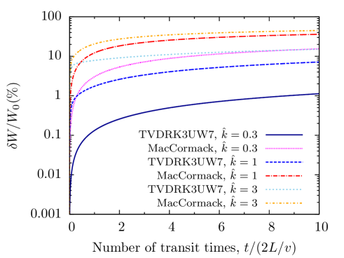
Figure 1: Energy conservation for the MacCormack and the TVDRK3UW7 schemes for the linear advection test problem defined in Equations (73–74). The $x$-axis is the time normalized by the transit time across the simulation box, $2L/v$. The $y$-axis is the variation in energy ($\delta W$) normalized by the initial energy, $W_{0}$. The parameter $\hat{k}=k\Delta z=2\pi/n_{p}$, where $n_{p}$ is the number of grid points per wavelength.

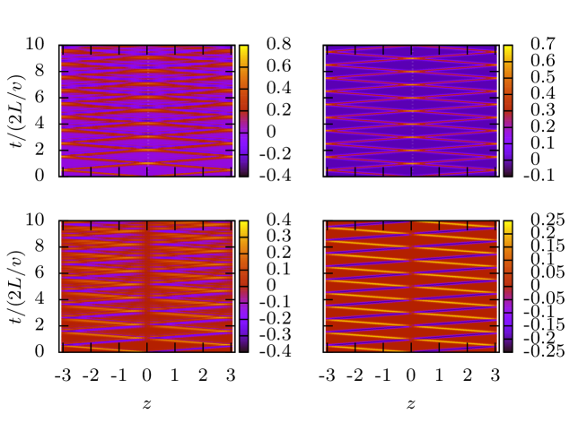
Figure 2: Results from the linear advection test problem of section 7.1. Contour plots of the time evolution of $A_{\parallel}$ (top) and $n_{e}$ (bottom) using the MacCormack scheme (left panels) and the TVDRK3UW7 scheme (right panels), for the case $\hat{k}=1$. The MacCormack scheme is seen to introduce strong Gibbs oscillations, which are remarkably minimized by the TVDRK3UW7 scheme.

Besides much better energy conservation properties, we find the TVDRK3UW7 scheme to be very robust against spurious Gibbs oscillations, even though it is not a shock-capturing scheme. This is clearly visible in Figure 2, where we plot the time history of the profiles of $A_{\parallel}$ and $n_{e}$ obtained with both schemes for $\hat{k}=1$. As can be seen, the TVDRK3UW7 scheme advects the initial condition with no visible deterioration, unlike the MacCormack scheme.

7.2 Linear Kinetic Alfvén Wave

The linearisation of equations (7–9) in the collisionless limit yields the kinetic Alfvén wave dispersion relation [21]:

$$\left[\zeta^{2}-\frac{\tau}{Z}\frac{k_{\perp}^{2}d_{e}^{2}/2}{1-\Gamma_{0}(k_{\perp}^{2}\rho_{i}^{2}/2)}\right]\left[1+\zeta Z(\zeta)\right]=\frac{1}{2}k_{\perp}^{2}d_{e}^{2},$$ (76)

where $\zeta=\omega/|k_{\parallel}|v_{the}$, $Z(\zeta)$ is the plasma dispersion function and $k_{\perp}^{2}=k_{x}^{2}+k_{y}^{2}$.

On the left plot of Figure 3 we show a comparison between the analytical values of the frequencies and damping rates, obtained by solving equation (76), and those computed by Viriato setting the number of Hermite moments to $M=19$ and the number of grid points in the $z$-direction to $32$. Very good agreement is observed over several orders of magnitude of the electron skin depth, $d_{e}$; the maximum relative error, obtained for the highest value of $d_{e}$, is only a few percent. The right plot shows the values of the frequency and damping rate for $k_{\perp}d_{e}=1$ as a function of the number of Hermite moments. For $M\geq 9$ the damping rate converges to the analytical value ($-\gamma=0.2331$), whereas for $\omega$ very little dependence on $M$ is observed.

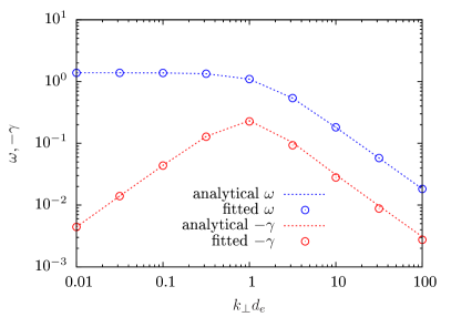
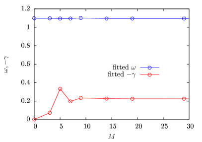
Figure 3: Left: Frequency and damping rate of the kinetic Alfvén wave (KAW), in units of $\tau_{A}$, at fixed $k_{\perp}\rho_{i}=1$, $\tau=1$, $M=19$, as a function of the electron skin-depth $d_{e}=c/\omega_{pe}$. Lines are the exact solution of the analytical dispersion relation, equation (76), whereas data points are obtained from Viriato. Right: KAW frequency and damping rate obtained from Viriato for fixed $k_{\perp}d_{e}=1$, as a function of the total number of Hermite moments kept, $M$.

7.3 Tearing Mode

The tearing mode [65] is a fundamental plasma instability driven by a background current gradient. Tearing leads to the opening, growth and saturation of (one or more) magnetic island(s) via the reconnection of a background magnetic field. It is of intrinsic interest to magnetic confinement fusion devices, where it occurs either in standard or modified form (i.e., neoclassical tearing, microtearing). It also represents the most basic paradigm for studies of magnetic reconnection.

In this section, we present the results of a linear benchmark of Viriato against the gyrokinetic code AstroGK [66] for the tearing mode problem. We consider an in-plane magnetic equilibrium configuration given by $B_{y,eq}=-dA_{\parallel,eq}/dx$, with $A_{\parallel,eq}=A_{\parallel 0}/\cosh^{2}(x/a)$, with $a$ the normalizing equilibrium scale length. The simulations are performed in a doubly periodic box of dimensions $L_{x}\times L_{y}$, with $L_{x}/a=2\pi$ and $L_{y}=2.5\pi$, such that $\hat{k}_{y}=2\pi a/L_{y}$ yields the tearing instability parameter $\Delta^{\prime}a=2(5-\hat{k}_{y}^{2})(3+\hat{k}_{y}^{2})/(\hat{k}_{y}^{2}\sqrt{4+\hat{k}_{y}^{2}})\approx 23$. Other parameters are $\rho_{i}/a=0.2$, $\tau=1$, $d_{e}/a=0.037$. All Viriato simulations keep $M=10$.

Figure 4 shows a plot of the linear growth rate of the tearing mode as a function of the Lundquist number $S=av_{A}/\eta$. The $S=\infty$ case is obtained by setting $\eta=0$, in which case the tearing mode is collisionless, i.e., the frozen-flux condition is broken by electron inertia instead. Calculations with AstroGK are done at three different values of $\beta_{e}$ and mass ratio: $(\beta_{e},m_{e}/m_{i})=(0.3,0.01),~{}(0.075,0.0025),~{}(0.01875,6.25\times 10^{-4})$ (crosses, squares and circles, respectively; this is the same data as plotted in Fig. 2 of Ref. [18]). As seen, the agreement between the two codes improves for smaller $\beta_{e}$, and is rather good for the smallest value of $\beta_{e}=0.01875$. Though it is expected that gyrokinetics will converge to KREHM as $\beta_{e}$ is decreased, we note that, at least in this particular case, agreement is achieved for $\beta_{e}$ substantially larger than $m_{e}/m_{i}$ (a factor of $30$), suggesting that KREHM may remain a reasonable approximation to the plasma dynamics outside its strict asymptotic limit of validity set by the requirement $\beta_{e}\sim m_{e}/m_{i}$.

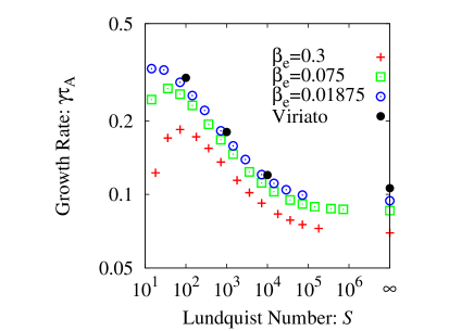
Figure 4: Tearing mode growth rate as a function of the Lundquist number. Figure shows a comparison between the results obtained with the gyrokinetic code AstroGK [66] for varying values of $\beta_{e}$ and Viriato. As expected, good agreement is obtained in the small $\beta_{e}$ limit.

A nonlinear benchmark is provided by the comparison of the tearing mode saturation amplitude with the prediction of MHD theory [67, 68, 69]. This was reported in Ref. [26], where it is shown that Viriato accurately reproduces the theoretical prediction in the parameter region where such prediction is valid [i.e., for $\Delta^{\prime}a\sim 1$ and as long as islands are larger than the kinetic scales of the problem ($\rho_{i},~{}\rho_{s},~{}d_{e}$)].

Finally, see also Figs. 1 and 3 of Ref. [70] for more direct comparisons between Viriato and AstroGK in the linear and nonlinear regime of a collisionless tearing mode simulation.

7.4 Orszag-Tang vortex problem

The Orszag-Tang (OT) vortex problem [71] is a standard nonlinear test for fluid codes, and a basic paradigm in investigations of decaying MHD turbulence [71, 72, 73, 74]. Here we present results from a series of 2D and 3D runs, including a kinetic case. For easy reference, we summarise the main parameters of each simulation performed in Table 1.

Run	Dim.	#Gridpoints	$\rho_{i}/a$	Dealiasing	Hyper-diss.?
A	2D	$2048^{2}$	0	$2/3$’s rule	no
A1	2D	$2048^{2}$	0	$2/3$’s rule	yes
B	2D	$2048^{2}$	0	Hou-Li	no
B1	2D	$2048^{2}$	0	Hou-Li	yes
C	3D	$512^{3}$	0	Hou-Li	yes
D	3D	$256^{3}$	2	Hou-Li	yes
E	3+1D	$256^{3}$	2	Hou-Li	yes

Table 1: Main parameters for decaying turbulence runs [with the Orszag-Tang-type initial conditions of equations (77–78) for the 2D runs, and of equations (81–82) for the 3D runs]. In all cases, $\rho_{s}=\rho_{i}$ and $d_{e}=0$. Run E also includes $20$ Hermite moments.

7.4.1 2D simulations of the OT vortex problem

To avoid an overly symmetric initial configuration, we adopt the modification of OT initial conditions proposed in Ref. [72], namely:

$$\Phi(x,y)=\cos(2\pi x/L_{x}+1.4)+\cos(2\pi y/L_{y}+0.5),$$ (77)

$$\Psi(x,y)=\cos(4\pi x/L_{x}+2.3)+\cos(2\pi y/L_{y}+4.1).$$ (78)

The runs are performed on a box of dimensions $L_{x}=L_{y}=2\pi$, at a resolution of $N_{x}\times N_{y}=2048^{2}$ collocation points. In the cases where no hyper-dissipation is used (runs A and B), the resistivity is set to $\eta=10^{-3}$, and the magnetic Prandtl number $Pm=\nu/\eta=1$. The kinetic scales $\rho_{i},~{}\rho_{s},~{}d_{e}$ are set to zero, so this is strictly a RMHD run.

Magnetic ($E_{M}$) and kinetic ($E_{K}$) energy time traces for runs A and B are shown on the left-hand panel of Figure 5. We compare the results obtained using the Hou-Li high order Fourier filter, equation (54), with those obtained with the standard $2/3$’s dealiasing rule of Orszag [56], equation (53). The agreement between the two sets of results is perfect, demonstrating that the Hou-Li filter does as good a job at conserving energy as the $2/3$’s rule.

The right-hand panel shows the time trace of the energy dissipation, normalized by the instantaneous total energy, i.e.,

$$\frac{D}{W}\equiv\frac{\int dV(\eta j^{2}+\nu\omega^{2})}{\frac{1}{2}\int dV(B^{2}+u^{2})}.$$ (79)

Since no energy is being injected into the system, the RMHD equations should obey the conservation relation

$$\frac{dW}{dt}=-D.$$ (80)

In order to demonstrate the accuracy of the code, we overplot a time trace of $-1/WdW/dt$. The very good agreement between the two curves is manifest; in this particular run, equation (80) is satisfied to better than $0.1\%$.

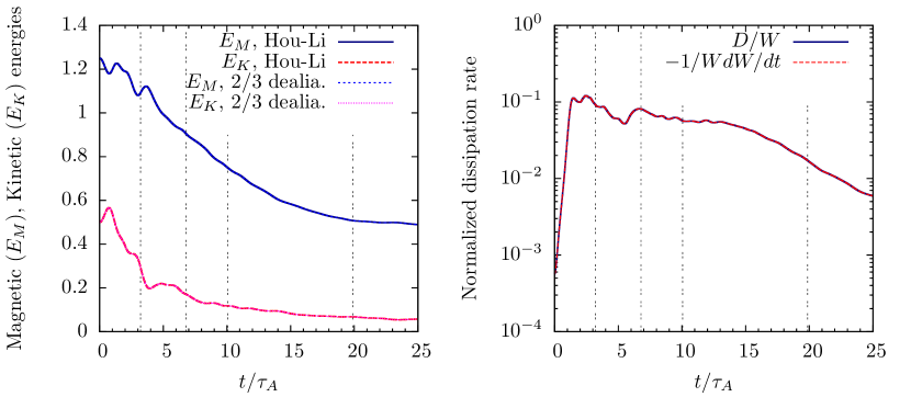
Figure 5: Runs A and B. Left panel: Time traces of the magnetic ($E_{M}$) and kinetic ($E_{k}$) energies, obtained from runs with different dealiasing methods: “Hou-Li” uses the high-order Fourier filter of Ref. [52], given by equation (54); “$2/3$ dealia.” uses the usual $2/3$’s rule of Ref. [56], equation (53). Right panel: Time trace of the energy dissipation rate (for the Hou-Li run), normalized by the instantaneous total energy, $D/W$. Overplotted is $-1/WdW/dt$: code conserves energy to better than $0.1\%$ in this run. The vertical dotted lines identify the times at which the contours of Figure 6 and spectra of Figure 7 are plotted.

Contour plots of current and vorticity (i.e., $\nabla^{2}_{\perp}\Phi$) at the times identified by the vertical lines in Figure 5 are plotted in Figure 6 (top and bottom rows, respectively). The formation of sharp current and vorticy sheets is observed, as expected. At $t/\tau_{A}=10.0$ one can observe a plasmoid [75, 76] erupting from the current sheet on the lower right-hand corner of the plot, in what is perhaps the small-scale version of the observations reported in Ref. [77]. The role of the tearing instability of current sheets in 2D decaying turbulence has been previously discussed in Refs. [72, 74].

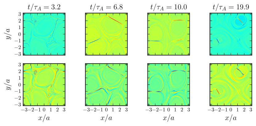
Figure 6: Run B (2D). Contour plots of current (top row) and vorticity (bottom row) at different times (identified by the vertical lines in Figure 5).

Figure 7 shows the total energy spectra obtained from the simulation with the Hou-Li filter (run B), taken at the times identified by the vertical lines in Figure 5. There is no evidence of pile-up (bottleneck) at the small scales (we note that the only dissipation terms present in this simulation are the standard laplacian resistivity and viscosity, i.e., there is no hyper-dissipation). Due to the relatively large values of the dissipation coefficients used in this simulation, the inertial range is very limited and it is not possible to clearly fit a unique power law; for reference, $k_{\perp}^{-3/2}$ is indicated in Figure 7, following the Iroshnikov-Kraichnan prediction [78, 79], and its numerical confirmation reported in Refs. [72, 74] (although steeper power-laws $\sim k_{\perp}^{-5/2}$ have also been reported in the literature [80, 59]).

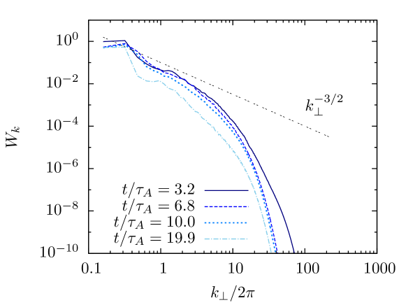
Figure 7: Run B (2D). Total energy spectra at different times (identified by the vertical lines in Figure 5). A $k_{\perp}^{-3/2}$ slope is shown for reference.

A much longer and cleaner inertial range is obtained by replacing the standard (laplacian) dissipation terms with hyper-dissipation (runs A1 and B1). In that case, the spectra shown in Figure 8 are obtained; the inertial range now shows an excellent agreement with the power-law slope of $-3/2$. Note also the extended inertial range obtained when the Hou-Li filter is used (B1) instead of the standard $2/3$’s dealiasing.

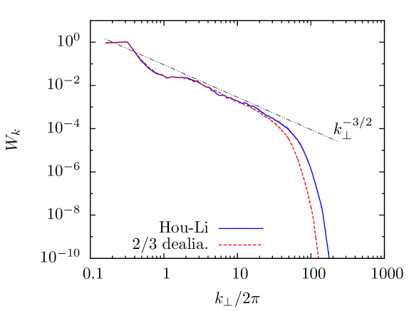
Figure 8: Runs A1 and B1 (2D). Total energy spectra at $t/\tau_{A}\approx 6.0$ obtained with the Hou-Li filter (blue, full line) and with the standard $2/3$’s dealising rule (red, dashed line). The Hou-Li method results in an extended inertial range for the same number of collocation points, as expected. Neither spectra shows signs of energy pile-up at the small scales. The power-law $k_{\perp}^{-3/2}$ is indicated for reference.

7.4.2 3D simulations of the OT vortex problem

For the 3D simulations the initial conditions differ from the 2D case only in that they are modulated in the $z$-direction, as follows:

$$\Phi(x,y)=\left[\cos(2\pi x/L_{x}+1.4)+\cos(2\pi y/L_{y}+0.5)\right]\sin(2\pi z/L_{z}),$$ (81)

$$\Psi(x,y)=\left[\cos(4\pi x/L_{x}+2.3)+\cos(2\pi y/L_{y}+4.1)\right]\cos(2\pi z/L_{z}).$$ (82)

We perform three different runs with these initial conditions (runs C, D and E). The first (run C) is just a straightforward extension to 3D of run B1, except now with a resolution of $N_{x}\times N_{y}\times N_{z}=512^{3}$. The second (run D) is designed to look at sub-ion-Larmor radius turbulence (i.e., kinetic Alfvén wave turbulence); thus we set $\rho_{i}/a=2,~{}d_{e}/a=0.01$, where $a=L_{x}/(2\pi)$, and $\tau=1$. The resolution in this case is $N_{x}\times N_{y}\times N_{z}=256^{3}$ (we use a smaller resolution here because the timestep, which is set by the CFL condition, is now also smaller, due to the dispersive nature of the kinetic Alfvén waves). Finally, run E also includes the velocity-space dependence, represented with $20$ Hermite moments (meaning that it differs from run D in that the electrons are no longer isothermal, i.e., $g_{e}\neq 0$)

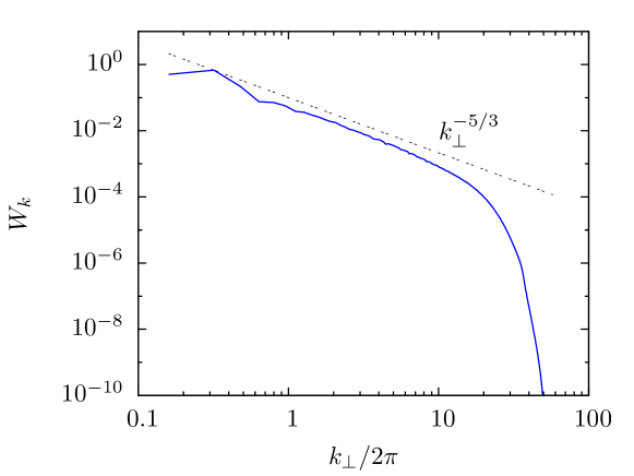
Figure 9: Run C (3D). Total energy spectra at $t/\tau_{A}\approx 4.0$. A $k_{\perp}^{-5/3}$ slope is shown for reference.

The total energy spectrum obtained for run C is shown in Figure 9. The inertial range shows very good agreement with the Goldreich-Sridhar $k^{-5/3}$ power law [81] and again is clean of bottleneck effects.

Figure 10 shows the magnetic, kinetic and electric energy spectra for run D, where we are now focussing on sub-ion Larmor radius scales. The slopes indicated refer to several power laws that have been widely discussed in the literature. In particular, we see that the separation between electric and magnetic energy scalings, occurring at around $(k_{\perp}/2\pi)\rho_{i}\sim 1$, agrees quite well with the solar wind observations reported by Bale et al. [82] and with the gyrokinetic simulations of Howes et al. [13]. However, instead of the $-7/3$ power law for the magnetic energy suggested in those works (discussed in more detail in Ref. [14]), we see that our data seems to more closely fit a $-8/3$ scaling, which is a better fit to the $-2.8$ slope often reported in observations (e.g., [83]) and in agreement with the recent work of Boldyrev and Perez [84] on strong kinetic Alfvénic turbulence.

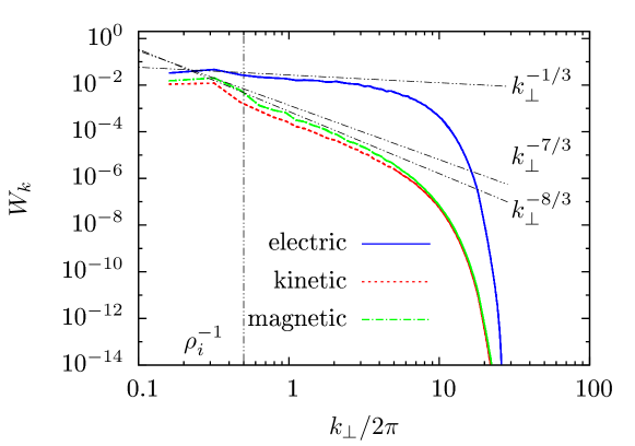
Figure 10: Run D (3D). Spectra for decaying turbulence [with OT-like initial conditions, equations (81–82)] at $t/\tau_{A}\approx 2.2$. The blue (full) line represents the perpendicular electric energy spectrum; the red (dashed) line is the perpendicular magnetic field energy and the green (dash-dot) line is the kinetic energy. The slopes $k_{\perp}^{-1/3}$, $k_{\perp}^{-7/3}$ and $k_{\perp}^{-8/3}$ are indicated for reference (see text for discussion). The vertical line indicates the ion Larmor radius scale.

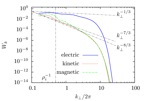
Figure 11: Run E (3D, with $20$ Hermite moments). Spectra at $t/\tau_{A}\approx 2.2$ for OT-decaying kinetic turbulence. Lines represent the same quantities as in Figure 10. See text for a discussion of the power laws indicated.

Figure 11 again shows energy spectra, this time for run E, which differs from run D in that it also includes Hermite moments (i.e., it is a fully kinetic run, whereas D assumes isothermal electrons, $g_{e}=0$). Comparing the magnetic spectra in the two cases (i.e, runs D and E, both drawn at the same time), we see that its values increase at the larger (spatial) scales when adding the Hermite moments, by about an order of magnitude, and run E’s spectrum seems to be somewhat steeper than $-8/3$. Such differences may be due to Landau damping, which is present in run E, but absent in run D. The Hermite spectrum (i.e., the electron free energy spectrum, $E_{m}=|g_{m}^{2}|/2$) for run E is shown in Figure 12, at different times. A $-1/2$ slope is indicated for reference; this is the inertial-range slope predicted by Zocco & Schekochihin [21] for the linear phase-mixing of Kinetic Alfvén waves. Since the number of Hermite moments ($20$) used is quite small we get an equivalently limited inertial range, and thus the agreement with the $-1/2$ slope can only be regarded as indicative; however, this tentative agreement lends credence to the idea that Landau damping may be playing a significant role in this simulation. A detailed analysis of kinetic turbulence in the KREHM framework and, in particular, of the relative importance of the different energy dissipation mechanisms available, will be the subject of a future publication.

Finally, for completeness we show in Figure 13 contour plots of the electron parallel velocity, $u_{e\parallel}$, and of the density perturbations, $n_{e}$, taken at the same time as the spectra of Figure 11 ($t/\tau_{A}\approx 2.2$).

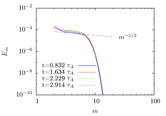
Figure 12: Run E (3D, with $20$ Hermite moments). Electron free-energy spectra $E_{m}=|g_{m}^{2}/2|$ at different times. An indicative power law of $m^{-1/2}$ for the inertial range is also shown [21].

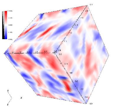
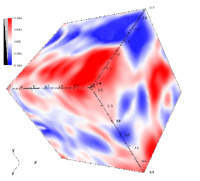
Figure 13: Run E: contour plots of the parallel electron velocity, $u_{e\parallel}$ (left), and density perturbations $n_{e}$ (right), at $t/\tau_{A}\approx 2.2$.

7.5 Collisionless damping of slow modes

We turn now to a benchmark of Viriato’s implementation of the KRMHD equations. Linearly, slow modes in KRMHD are subject to collisionless damping via the Barnes damping mechanism [85]. An initial perturbation damps at a rate that depends on the parameter $\Lambda$. If slow mode fluctuations are constantly driven with an external force (this is achieved by adding a forcing term to Eq. (17)), then the system can be thought of as a plasma-kinetic Langevin equation. The mean-squared amplitude of the electrostatic potential for such a system reaches a steady-state saturation level, which can be derived analytically [44].

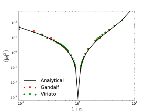
Figure 14: Steady-state amplitude of the electrostatic potential vs $1+\alpha$, where $\alpha=-1/\Lambda$. The solid line is the analytical prediction [44], the red crosses are numerical results calculated using Gandalf, and the green circles are calculated using Viriato.

In figure 14, we compare the steady-state saturation levels computed using Viriato with the analytical predictions, and the numerical results from another code — Gandalf (a fully spectral GPU code that solves the KRMHD equations). Slow mode fluctuations were driven using white noise forcing which injected energy into the system with unit power. The spatial resolution was set to $N_{x}\times N_{y}\times N_{z}=32^{3}$; $20$ Hermite moments of the distribution function were retained, $M=20$. The system was evolved until it reached a steady state. The saturation level was then calculated by averaging over the steady state fluctuations for a few Alfvén times. It can be seen that the saturation amplitudes obtained using Viriato are in near perfect agreement with those calculated by Gandalf, as well as with the analytical prediction.

8 Performance

Viriato has been used on a variety of computing clusters, with different architectures. It is quite easy to install and run, having dependencies only on standard, widely-used libraries such as LAPACK [63] and FFTW [87]. Its parallelization relies on standard MPI routines.

As described in detail in Section 6, the direction parallel to the field can be integrated by two different numerical methods, both of them fairly scalable, in terms of parallel performance. In contrast, the direction perpendicular to ${\bf B}_{0}$ uses standard pseudospectral techniques, which are plagued with well-known limits on scalability, due to the inherent non-locality of Fourier transforms. For this reason, if one wishes to increase the number of processors for a given computation, it is more effective to do so by increasing the ratio between the number of processes for the parallel direction and the number of processes in the perpendicular direction.

The results of such a test, made on the Helios machine (an Intel Xeon E5 cluster), can be seen on Figure 15, where the MacCormack method was used in the parallel direction. The initial conditions are the 3D Orszag-Tang vortex given by equations (81–82), with $15$ Hermite moments. We look at strong scaling, keeping the problem size fixed and varying the number of MPI processes, mainly in the parallel direction. This produces a supralinear scaling, which breaks down after $1024$ cores for the $256^{3}$ case and at $\sim 4096$ cores for the $512^{3}$ one. Similar results have been obtained on other clusters, such as Stampede (a mixed Intel Xeon E5 and Intel Xeon Phi Coprocessor cluster), Hopper (a Cray XE6) and Edison (a Cray XC30.

Currently ongoing optimization work includes parallelizing the computation of the Hermite moments’ via OpenMP.

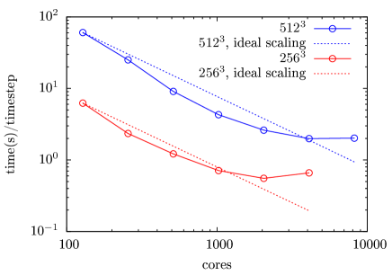
Figure 15: Viriato timings measured on the Helios cluster, for two different fixed problem sizes (strong scaling). A supralinear trend can be observed, which breaks down after $1024$ cores for the $256^{3}$ case and at $\sim 4096$ cores for the $512^{3}$ one. The vertical axis gives the wall-clock time (in seconds) spent per timestep.

9 Conclusions

This paper describes Viriato, a novel code developed to investigate strongly magnetised, weakly-collisional, fluid-kinetic plasma dynamics in (2D or 3D) slab geometry. Viriato solves two different sets of equations: the Kinetic Reduced Electron Heating Model (KREHM) of Zocco & Schekochihin [21] (which simplifies to conventional reduced-MHD [27, 28] in the appropriate limit) and the Kinetic Reduced MHD (KRMHD) equations of Schekochihin et al. [14].

The main numerical methods and the overall algorithm are described. A noteworthy feature of Viriato is its spectral representation of velocity-space, achieved via a Hermite expansion of the distribution function, as proposed in [21] for KREHM and in [44] for the KRMHD equations. This representation has the attractive property of converting the kinetic equation for the distribution function into a coupled set of fluid-like equations for each Hermite polynomial coefficient — the advantage being that such equations are numerically more convenient to solve than the kinetic equation where they stem from. On the other hand, the Hermite expansion introduces a closure problem (in the sense that the equation for the Hermite coefficient of order $m$ couples to that of order $m+1$). To address this problem, we present a nonlinear, asymptotically rigorous closure whose validity requires only that collisions are finite, but otherwise as small as required. Naturally, the smaller the collision frequency the higher the number of Hermite moments that need to be kept to guarantee the accuracy of the closure. Realistic values of the collision frequency in the systems that are of primary interest to us (e.g., modern fusion devices, space and astrophysical environments) lead to impractically large number of moments. The adoption of a hyper-collision operator (the direct translation into Hermite space of the usual hyper-diffusion operators used in (Fourier) $k$-space) allows us to deal with this problem. Together with a pseudo-spectral representation of the plane perpendicular to the background magnetic field, and the option of a spectral-like algorithm for the dynamics along the field, the Hermite representation of velocity space implies that Viriato is ideally suited to the investigation of magnetised kinetic plasma turbulence and magnetic reconnection, with the unique capability of allowing for the direct monitoring of energy flows in phase-space [26].

A series of linear and nonlinear numerical tests of Viriato is presented, with emphasis on Orszag-Tang-type decaying turbulence, both in the fluid and kinetic limits, where it is shown that Viriato recovers the theoretically expected power-law spectra. In this context, an interesting, novel result that warrants further investigation and will be discussed in a separate publication is the $\sim m^{-1/2}$ velocity-space (Hermite) spectrum that is obtained in the 3D kinetic (sub-ion Larmor radius scales) Orszag-Tang run presented in section 7.4.2 (see Figure 12). This particular form of the Hermite spectrum is indicative of linear phase mixing [21, 26] and suggests that this (and ensuing Landau damping) may be a key energy transfer mechanism in kinetic decaying turbulence.

Appendix A: Addition of a background electron temperature gradient

A recent paper by Zocco et al. [35] extends the KREHM model to include a background electron temperature gradient. This extension is also implemented in Viriato; results of ongoing investigations exploring different instabilities introduced by these terms (namely, the electron temperature gradient mode, and the microtearing instability) will be reported elsewhere. For completeness, we write below the KREHM equations with this extension in normalised form (see section 5 for the details of the normalisation adopted in Viriato). They are:

$$\frac{dn_{e}}{dt}=\left[A_{\parallel},\nabla^{2}_{\perp}A_{\parallel}\right]-\frac{\partial}{\partial z}\nabla^{2}_{\perp}A_{\parallel},$$ (83)

$$\frac{d}{dt}\left(A_{\parallel}-d_{e}^{2}\nabla^{2}_{\perp}A_{\parallel}\right)=\eta\nabla^{2}_{\perp}A_{\parallel}+\rho_{s}^{2}\left[n_{e}+\sqrt{2}g_{2},A_{\parallel}\right]-\frac{1}{\sqrt{2}}\frac{\rho_{s}}{d_{e}}\alpha_{Te}\frac{\partial A_{\parallel}}{\partial y}$$

$$\qquad\qquad-\frac{\partial\varphi}{\partial z}+\rho_{s}^{2}\frac{\partial}{\partial z}\left(n_{e}+\sqrt{2}g_{2}\right)$$ (84)

$$\frac{dg_{2}}{dt}=\sqrt{3}\frac{\rho_{s}}{d_{e}}\left\{\left[A_{\parallel},g_{3}\right]-\frac{\partial g_{3}}{\partial z}\right\}+\sqrt{2}\left\{\left[A_{\parallel},\nabla^{2}_{\perp}A_{\parallel}\right]-\frac{\partial}{\partial z}\nabla^{2}_{\perp}A_{\parallel}\right\}$$

$$\qquad\qquad-\frac{1}{2}\frac{1}{\rho_{s}d_{e}}\alpha_{Te}\frac{\partial\varphi}{\partial y},$$ (85)

$$\frac{dg_{m}}{dt}=\sqrt{m+1}\frac{\rho_{s}}{d_{e}}\left\{\left[A_{\parallel},g_{m+1}\right]-\frac{\partial g_{m+1}}{\partial z}\right\}+\sqrt{m}\frac{\rho_{s}}{d_{e}}\left\{\left[A_{\parallel},g_{m-1}\right]-\frac{\partial g_{m-1}}{\partial z}\right\}$$

$$\qquad\qquad-m\nu_{ei}g_{m}+\delta_{m,3}\frac{1}{2}\frac{1}{d_{e}^{2}}\alpha_{Te}\frac{\partial A_{\parallel}}{\partial y},\quad m>2,$$ (86)

where $\alpha_{Te}=\rho_{e}/L_{Te}L_{\parallel}/L_{\perp}$, with $\rho_{e}$ the electron Larmor radius and $L_{Te}$ the electron temperature gradient scale length.

References

-
[1]
R. Bruno, V. Carbone,
The solar wind as a
turbulence laboratory, Liv. Rev. Solar Phys. 2 (2005) 4.
doi:10.12942/lrsp-2005-4.
URL http://adsabs.harvard.edu/abs/2005LRSP....2....4B -
[2]
B. G. Elmegreen, J. Scalo,
Interstellar
Turbulence I: Observations and processes, Annu. Rev. Astron. Astrophys.
42 (1) (2004) 211–273.
doi:10.1146/annurev.astro.41.011802.094859.
URL http://www.annualreviews.org/doi/abs/10.1146/annurev.astro.41.011802.094859 - [3] K. Shibata, T. Magara, Solar Flares: Magnetohydrodynamic Processes, Liv. Rev. Solar Phys. 8 (2011) 6. doi:10.12942/lrsp-2011-6.
- [4] B. Haisch, K. T. Strong, M. Rodono, Flares on the Sun and other stars, Annu. Rev. Astron. Astrophys. 29 (1991) 275–324. doi:10.1146/annurev.aa.29.090191.001423.
-
[5]
D. A. Uzdensky,