CTP-SCU/2015006

Equivalence of open/closed strings

Peng Wang, Houwen Wu and Haitang Yang

Center for theoretical physics

Sichuan University

Chengdu, 610064, China

pengw, hyanga@scu.edu.cn, iverwu@stu.scu.edu.cn

Abstract

In this paper, we prove that the open and closed strings are $O(D,D)$ equivalent. The equivalence requires an AdS geometry near the boundaries. The $O(D,D)$ invariance is introduced into the Polyakov action by the Tseytlin’s action. Traditionally, there exist disconnected open-open or closed-closed configurations in the solution space of the Tseytlin’s action. The open-closed configuration is ruled out by the mixed terms of the dual fields. We show that, under some very general guidances, the dual fields are consistently decoupled if and only if the near horizon geometry is $AdS_{5}$. We then have open-closed and closed-open configurations in different limits of the distances of the $D3$-brane pairs. Inherited from the definition of the theory, these four configurations are of course related to each other by $O(D,D)$ transformations. We therefore conclude that both the open/closed relation and open/closed duality can be derived from $O(D,D)$ symmetries. We then demonstrate the open/closed relation does connect commutative open and closed strings. By analyzing the couplings of the configurations, the low energy effective limits of our results consequently predicts the AdS/CFT correspondence, Higher spin theory, weak gauge/weak gravity duality and a yet to be proposed strong gauge/strong gravity duality. Furthermore, we also have the Seiberg duality and a weak/strong gravitation duality as consequences of $O(D,D)$ symmetries.

1 Introduction

It is one of the most important tasks in modern physics to figure out the relations between gauge theory and gravity, the quantum and the classical theories. We claim string theory is the TOE, it is therefore expected to answer these questions. However, the primordial string theory is only defined in a perturbative way, the Polyakov action. We thus believe that the answers of these non-perturbative problems root in M-theory. Before touching the holy grail of M theory, some non-perturbative facts already emerge from the perturbative theories. We have the T-duality, which implies the equivalence of physics between the small and big tori, the S-duality, which unifies the strong and weak couplings, the U-duality, a combination of T- and S-dualities. The U-duality is the fundamental symmetry of M theory. These dualities are known as non-perturbative effects, and exist in the low energy effective theories. The T-duality can be realized as the discrete $O\left(d,d;\mathbb{Z}\right)$ symmety. The manifestly $O\left(d,d;\mathbb{Z}\right)$ invariant action is given in ref. [1]. The S-duality manifests $SL\left(2,\mathbb{R}\right)$ symmetry. The corresponding $SL\left(2,\mathbb{R}\right)$ invariant action can be found in ref. [2]. Since these dualities already show up in the low energy effective theories, it is unbelievable that they cannot be manifested in the world-sheet action. Since we still do not know how to define M theory, it is highly motivated to construct intermediate theories between the perturbative string theory and M theory, by introducing dualities into the world-sheet action. One can anticipate that these intermediate theories may provide answers to some of the non-perturbative effects.

Besides these dualities, there exist some amazing relations between open string and closed string theories. The first one is the open/closed relation, which connects the open/closed string metrics and couplings. The low energy effective partner of this relation is the Seiberg-Witten map [3] between commutative and non-commutative gauge theories. The second one is the open/closed string duality. It shows the equivalence between the one-loop open string amplitude and the tree-level closed string amplitude. Since in low energy limits, open strings represent gauge theories and closed strings denote gravity, based on the open/closed string duality, the gauge/gravity duality is conjectured when $N\rightarrow\infty$ [4]. The relation between open/closed string duality and gauge/gravity duality is addressed in [5]. As a realization of the gauge/gravity duality, the well-known AdS/CFT [6] identifies the strong gauge theory and weak gravity. It presents the correspondence between the quantum gravity in the bulk and gauge theory on the boundary. There is also a conjectured duality between the strong gravity and weak gauge theories, the Higher spin theory [7].

Let us recall some facts of M theory. M theory has five different limits or five string theories. We believe that these various string theories describe the same object from different perspectives. One of them is the type I string theory, which includes both open and closed strings. The other four string theories have closed strings only. Since they describe the same object, there must exist relations between closed strings and open strings on the level of M theory. On the other hand, we have known that the U-duality is a fundamental symmetry of M theory, which is identified as $E_{D}$ group. The U-duality groups and their maximal subgroups in various dimensions are summarized in Table (1) [8].

$D$	$E_{D}$	$H_{D}$
3	$SL\left(3\right)\times SL\left(2\right)$	$SO\left(3\right)\times SO\left(2\right)$
4	$SL\left(5\right)$	$SO\left(5\right)$
5	$SO\left(5,5\right)$	$SO\left(5\right)\times SO\left(5\right)$
6	$E_{6}$	$USp\left(8\right)$
7	$E_{7}$	$SU\left(8\right)$
8	$E_{8}$	$SO\left(16\right)$

Table 1: The U-duality group

It is inspiring to notice that in $D=5$, M theory has $SO\left(5,5\right)$ symmetry. Therefore, we have strong motivation to introduce the $O\left(D,D\right)$ symmetry into the Polyakov action to construct an intermediate theory between the primordial string theory and M theory. It may capture some non-perturbative properties of M theory. The $O\left(D,D\right)$ symmetry is a continuous symmetry for non-compact $D$ dimensional spacetime. After compactifying $d=D-n$ dimensions, the continuous $O\left(D,D\right)$ breaks into $O\left(n,n\right)\times O\left(d,d;\mathbb{Z}\right)$ group. The discrete $O\left(d,d;\mathbb{Z}\right)$ group is known as T-duality group in the compactified $d$ dimensional spacetime. The good news is that there is an available world-sheet action which manifests $O\left(D,D\right)$ symmetry, the Tseytlin’s action. This action sometimes is also named as double sigma model, built by Tseytlin [9] and developed in [10, 11].

The Tseytlin’s action was originally proposed for closed strings, where a set of fields $\tilde{X}$ dual to the ordinary $X$ is introduced to manifest $O(D,D)$ symmetry. It was found in [12] that non-commutative and commutative closed string theories can be unified in this theory. The low energy effective descendant is called double field theory [13, 14, 15, 16]. On the other hand, we showed in [17] that this action can be perfectly applied on open strings. The non-commutative and commutative open strings are unified precisely through the open/closed relation. In the low energy limit, they reduce to the non-commutative and commutative gauge theories, related by the Seiberg-Witten map [3]. It is puzzling that, in the open($X$)-open($\tilde{X}$) and closed($X$)-closed($\tilde{X}$) scenarios, there are lots of identical relations. In these two situations, the dual fields $X$ and $\tilde{X}$ must take the same boundary conditions, open-open or closed-closed, protected by the complete form of the boundary conditions. However, it is curious to ask:

• Is the open($X$)-closed($\tilde{X}$) configuration allowed?

• Why does the open/closed relation connect commutative/non-commutative theories in open-open configuration or closed-closed configuration but not relate theories in open-closed configuration, just as the name implies?

In any case, there are many clues of the equivalence of open strings and closed strings. The main purpose of this paper is to give affirmative answers to these questions. The point is that, there is a third boundary condition which looks blurry at a first sight, since it does not fix the string to be open or closed definitely. This actually is the good news. The bad news is obvious, we can do little without fixing to open or closed strings. However, once study the complete form of the boundary conditions carefully, we can find that what forbids the open-closed configuration is the mixed terms of $X$ and $\tilde{X}$. It is not hard to understand that if $X$ and $\tilde{X}$ are decoupled near the boundary, either of them is free to be open or closed. Originally, the metric in the Tseytlin’s action is totally flat, as that in Polyakov action. But since we are considering an $O(D,D)$ extension of the Polyakov action, we are certainly allowed to relax the metric to be spacetime dependent as long as the $O(D,D)$ covariance is preserved. We show that, the decoupling of $X$ and $\tilde{X}$ happens if and only if the near boundary geometry is $AdS_{5}$ from some general considerations! It should be emphasized that the decoupling of the dual fields only occurs near the boundary. In the bulk, $X$ and $\tilde{X}$ are related by first order differential equations, which is crucial to have difference to the Polyakov action. We then demonstrate that under different limits, there are open-closed and closed-open configurations, all of which are related by $O(D,D)$ transformations. The strength of the couplings of the low energy effective theories is determined by the distances between the $D$-brane pairs. We thus can analyze the symmetries or dualities of the various low energy effective theories. It turns out that all the relations we mentioned above: AdS/CFT, higher spin and weak gauge/weak gravity, strong gauge/strong gravity can be put into this framework and explained by $O(D,D)$ symmetries. There are also the weak/strong gauge duality known as the Seiberg duality and a weak/strong gravitation duality anticipated from our derivations. Therefore, all the currently known dualities are subsets of the $O(D,D)$ group.

The reminder of this paper is outlined as follows. In section 2, we show how to realize the open-closed configuration and give the transformations between all of the four configurations. The consequences of the low energy effective limits are addressed in section 3. Section 4 is the summary and discussion.

2 The equivalence of the open and closed strings

We start with the Tseytlin’s action

$$S=-\frac{1}{4\pi\alpha^{\prime}}\int_{\Sigma}\left(-\partial_{1}X^{M}\mathcal{H}_{MN}\partial_{1}X^{N}+\partial_{1}X^{M}\eta_{MN}\partial_{0}X^{N}\right),$$ (2.1)

where $\partial_{0}=\partial_{\tau}$, $\partial_{1}=\partial_{\sigma}$ and

$$\mathcal{H}_{MN}=\left(\begin{array}[]{cc}g&-gB^{-1}\\ B^{-1}g&g^{-1}-B^{-1}gB^{-1}\end{array}\right),\qquad\eta_{MN}=\left(\begin{array}[]{cc}0&1\\ 1&0\end{array}\right),\qquad X^{M}=\left(\begin{array}[]{c}X^{i}\\ \tilde{X}_{i}\end{array}\right),$$ (2.2)

where $M,N=1,2,\ldots,2D$ are $O\left(D,D\right)$ indices, $g$ is $D$ dimensional spacetime metric and $B$ is the anti-symmetric Kalb-Ramond field. This action manifests $O\left(D,D\right)$ symmetry, and the components are invariant under the $O\left(D,D\right)$ rotations: $\Omega\eta\varOmega^{T}=\eta$. The EOM and boundary conditions can be obtained by varying the action,

$$\delta S = -\frac{1}{2\pi\alpha^{\prime}}\int_{\Sigma}\delta X^{M}\partial_{1}\left(\mathcal{H}_{MN}\partial_{1}X^{N}-\eta_{MN}\partial_{0}X^{N}\right)$$ (2.3)

$$+\frac{1}{2\pi\alpha^{\prime}}\int_{\Sigma}\partial_{1}\left[\delta X^{M}\left(\mathcal{H}_{MN}\partial_{1}X^{N}-\frac{1}{2}\eta_{MN}\partial_{0}X^{N}\right)\right]$$

$$-\frac{1}{4\pi\alpha^{\prime}}\int_{\Sigma}\partial_{0}\left[\delta X^{N}\eta_{MN}\partial_{1}X^{M}\right]$$

$$+\frac{1}{4\pi\alpha^{\prime}}\int_{\Sigma}\delta X^{M}\partial_{1}X^{A}\partial_{M}\mathcal{H}_{AN}\partial_{1}X^{N},$$

where we kept the spacelike boundary for reasons becoming clear soon. For simplicity, we consider vanishing $B$ field at first. The EOM is

$$\partial_{1}\left(\mathcal{H}_{MN}\partial_{1}X^{N}-\eta_{MN}\partial_{0}X^{N}\right)=\frac{1}{2}\partial_{1}X^{A}\partial_{M}\mathcal{H}_{AN}\partial_{1}X^{N}.$$ (2.4)

It turns out that the annoying term on the right hand side of the EOM is irrelevant for almost all of the discussions in this paper. Later we will see that this term technically narrows down the choices of the metric. We thus set it vanishing and get

$$g_{ij}\partial_{1}X^{j}-\partial_{0}\tilde{X}_{i} = f_{1}\left(\tau\right),$$ (2.5)

$$g^{ij}\partial_{1}\tilde{X}_{j}-\partial_{0}X^{i} = f_{2}\left(\tau\right).$$ (2.6)

The boundary terms are:

$$\delta X^{i}\left(g_{ij}\partial_{1}X^{j}-\frac{1}{2}\partial_{0}\tilde{X}_{i}\right)+\delta\tilde{X}_{i}\left(g^{ij}\partial_{1}\tilde{X}_{j}-\frac{1}{2}\partial_{0}X^{i}\right)\Bigg{|}_{\sigma} = 0,$$ (2.7)

$$\delta X^{i}\partial_{1}\tilde{X}_{i}+\delta\tilde{X}_{i}\partial_{1}X^{i}|_{\tau} = 0,$$ (2.8)

where $|_{\sigma}$ stands for the timelike boundaries swept by the end points of the string, and $|_{\tau}$ denotes the initial and final states. The $|_{\tau}$ boundary was used to construct D-branes in closed string theory in [18]. It is not hard to see that both $X$ and $\tilde{X}$ can represent closed strings (closed-closed). In this scenario, there is no boundary and we can set $f_{i}(\tau)=0$ by redefining $X$ and $\tilde{X}$. In [17, 19], we showed that $X$ and $\tilde{X}$ can also describe open strings (open-open) by setting

$$\delta X^{i}|_{\sigma}=\left(g^{ij}\partial_{1}\tilde{X}_{j}-\frac{1}{2}\partial_{0}X^{i}\right)\Bigg{|}_{\sigma}=0\qquad\Longrightarrow\qquad\partial_{0}X|_{\sigma}=\partial_{1}\tilde{X}|_{\sigma}=0,$$ (2.9)

or

$$\delta\tilde{X}_{i}|_{\sigma}=\left(g_{ij}\partial_{1}X^{j}-\frac{1}{2}\partial_{0}\tilde{X}_{i}\right)\Bigg{|}_{\sigma}=0\qquad\Longrightarrow\qquad\partial_{1}X|_{\sigma}=\partial_{0}\tilde{X}|_{\sigma}=0.$$ (2.10)

In this case, $f_{i}(\tau)$ can also be absorbed into $X$ and $\tilde{X}$. In these two situations, it proves that the Tseytlin’s theory can reduce to the Polyakov action. It is then tempting to ask the question: Is it possible that $X$ represents open strings but $\tilde{X}$ describes closed strings simultaneously, or vice versa? Since $X$ and $\tilde{X}$ are related by $O(D,D)$ transformations, if this configuration is permitted, it becomes possible to explain and furthermore explore the various dualities and relations between open and closed strings. As we promised in the introduction, we are going to show that this configuration does exist.

2.1 Open-closed configurations

Referring to eqn. (2.7), in addition to the closed-closed and open-open boundary conditions, there is one more $O(D,D)$ covariant boundary condition

$$\left(g_{ij}\partial_{1}X^{j}-\frac{1}{2}\partial_{0}\tilde{X}_{i}\right)\Bigg{|}_{\sigma}=\left(g^{ij}\partial_{1}\tilde{X}_{j}-\frac{1}{2}\partial_{0}X^{i}\right)\Bigg{|}_{\sigma}=0.$$ (2.11)

This boundary condition is neither open string boundary nor closed string one. It proves that under this boundary condition, the Tseytlin’s action can not reduce to the Polyakov action and it is impossible to remove half of the degrees of freedom by their EOM. This observation implies that the Tseytlin’s theory is more general than the Polyakov one. Applying the EOM (2.6) on the boundary (2.11), we obtain

$$f_{1}\left(\tau\right)=-\frac{1}{2}\partial_{0}\tilde{X}\Big{|}_{\sigma},\quad\quad f_{2}\left(\tau\right)=-\frac{1}{2}\partial_{0}X\Big{|}_{\sigma}.$$ (2.12)

We thus can again absorb $f_{i}\left(\tau\right)$ by shifting $X$ and $\tilde{X}$,

$$\tilde{X}\to\tilde{X}-\int d\tau f_{1}\left(\tau\right),\quad\quad X\to X-\int d\tau f_{2}\left(\tau\right).$$ (2.13)

Then the decoupled second order EOM is

$$(\partial_{1}\,^{2}-\partial_{0}\,^{2})X = 0,$$

$$(\partial_{1}\,^{2}-\partial_{0}\,^{2})\tilde{X} = 0,$$ (2.14)

with the first order constraint,

$$g\partial_{1}X-\partial_{0}\tilde{X} = 0,$$

$$g^{-1}\partial_{1}\tilde{X}-\partial_{0}X = 0,$$ (2.15)

and the boundary conditions,

$$\delta X^{i}\left(g_{ij}\partial_{1}X^{j}-\partial_{0}\tilde{X}_{i}\right)+\delta\tilde{X}_{i}\left(g^{ij}\partial_{1}\tilde{X}_{j}-\partial_{0}X^{i}\right)|_{\sigma} = 0,$$

$$g_{ij}\delta X^{i}\partial_{0}X^{j}+g^{ij}\delta\tilde{X}_{i}\partial_{0}\tilde{X}_{j}|_{\tau} = 0,$$ (2.16)

where we applied the constraint (2.15) on the spacelike boundaries. Note due to the shift of $X$ and $\tilde{X}$, the factor $1/2$ in the boundary conditions (2.11) disappear, and they are the same as the first order EOM. To see the picture clearer, we consider the string propagating between two D-$p$ branes. We use the notations:

$$\mu,\nu,\ldots = 0,\ldots,p,$$

$$a,b,\ldots = p+1,\ldots,D-1.$$ (2.17)

The boundary conditions (2.16) become

$$\delta X^{a}\left(g_{ab}\partial_{1}X^{b}-\partial_{0}\tilde{X}_{a}\right)+\delta\tilde{X}_{a}\left(g^{ab}\partial_{1}\tilde{X}_{b}-\partial_{0}X^{a}\right)$$

$$+\delta X^{\mu}\left(g_{\mu\nu}\partial_{1}X^{\nu}-\partial_{0}\tilde{X}_{\mu}\right)+\delta\tilde{X}_{\mu}\left(g^{\mu\nu}\partial_{1}\tilde{X}_{\nu}-\partial_{0}X^{\mu}\right)|_{\sigma} = 0,$$

$$g_{ab}\delta X^{a}\partial_{0}X^{b}+g^{ab}\delta\tilde{X}_{a}\partial_{0}\tilde{X}_{b}$$

$$+g_{\mu\nu}\delta X^{\mu}\partial_{0}X^{\nu}+g^{\mu\nu}\delta\tilde{X}_{\mu}\partial_{0}\tilde{X}_{\nu}|_{\tau} = 0.$$ (2.18)

At a first glance, there can only be closed-closed or open-open configurations. However, what forbid the open-closed configuration are the cross terms between $X$ and $\tilde{X}$. Once $X$ and $\tilde{X}$ are decoupled, each of them is free to be open or closed, which leads to the open-closed configuration! Such a case happens when $g_{\mu\nu}\gg 1$ or $g_{\mu\nu}\ll 1$, where we used the fact that $g_{ab}$ and $g_{\mu\nu}$ are reciprocal in D-brane theory and $g_{a\mu}=0$. In the original Tseytlin’s theory, the metric was set to be flat. However, we are trying to generalized the Polyakov action to an $O(D,D)$ invariant theory. Following the same pattern as Polyakov action to the nonlinear sigma model, we certainly can go a little bit further to have a nonlinear double sigma model, as long as the $O(D,D)$ invariance is preserved. On the other hand, it is well-known that the symmetry group of M-Theory in five dimensional spacetime is $SO(5,5)$, we thus choose $D=5$. Moreover, it is generically true that the metric on D-branes is conformally flat. Therefore, the near-horizon metric is almost fixed to be

$$ds^{2}=f\left(r\right)\eta_{\mu\nu}dx^{\mu}dx^{\nu}+f\left(r\right)^{-1}dr^{2},\qquad g_{\mu\nu}=f\left(r\right)\eta_{\mu\nu},\qquad g_{ab}=f\left(r\right)^{-1},$$ (2.19)

where $dr$ is the normal direction to the D-branes. This metric is nothing but the geometry of $AdS_{5}$ once requiring it is consistent with the Einstein equation,

$$ds^{2}=\frac{r^{2}}{c^{2}}\eta_{\mu\nu}dx^{\mu}dx^{\nu}+\frac{c^{2}}{r^{2}}dr^{2},$$ (2.20)

where $c$ is the radius of the AdS. It must be emphasized that we only need the decoupling of $X$ and $\tilde{X}$ near the boundary. In the bulk, $X$ and $\tilde{X}$ are coupled. Decoupling of $X$ and $\tilde{X}$ in the bulk will make the configuration unphysical as indicated by the EOM (2.15). This is very different from the story of Polyakov action. In Polyakov theory, there does not exist intermediate mixed open-closed states. Therefore, it is impossible to have different configurations in different limits. We now show how the open-closed configuration emerges under the limits. Substituting the metric into the boundary condition (2.18) and setting $r\gg c$, we get

$$\delta\tilde{X}_{a}\left(\frac{r^{2}}{c^{2}}\delta^{ab}\partial_{1}\tilde{X}_{b}\right)+\delta X^{\mu}\left(\frac{r^{2}}{c^{2}}\eta_{\mu\nu}\partial_{1}X^{\nu}\right)|_{\sigma} = 0,$$ (2.21)

$$\frac{r^{2}}{c^{2}}\delta^{ab}\delta\tilde{X}_{a}\partial_{0}\tilde{X}_{b}+\frac{r^{2}}{c^{2}}\eta_{\mu\nu}\delta X^{\mu}\partial_{0}X^{\nu}|_{\tau} = 0.$$ (2.22)

From the second term of eqn. (2.21), we can choose

$$\eta_{\mu\nu}\partial_{1}X^{\nu}|_{\sigma}=0,$$ (2.23)

which makes $X$ is a description of open strings. To cancel the second term on (2.22), we may choose

$$X\left(\sigma,\tau\right)=X\left(\sigma,\tau+2\pi t\right),$$ (2.24)

which represents a periodic motion of an open string. $t$ runs from $0$ to $\infty$. Bear in mind that $t$ is not a world-sheet coordinate, but a spacetime coordinate. As a matter of fact, non-compact time evolution also fits the boundary condition, since in this case, as we always do, there is no boundary on the temporal direction for open strings and the second term of eqn. (2.22) identically vanishes. The discussion on this topology is parallel to the compact case. We will mention the differences at the right places. In this paper, we focus on the compact topology in order to make the picture easier to understand.

From the first term of eqn. (2.22), we set

$$\tilde{X}_{b}|_{\tau}=\tilde{Y}_{b},$$ (2.25)

which makes $\tilde{X}$ represent a closed string. The first term of eqn (2.21) vanishes since there is no timelike boundary for closed strings and we have

$$\tilde{X}(\sigma,\tau)=\tilde{X}(\sigma+2\pi,\tau)$$ (2.26)

The consistent choices for $X^{a}|_{\sigma}$ and $\tilde{X}_{\mu}|_{\tau}$ are therefore

$$X^{a}|_{\sigma} = Y^{a},$$

$$\eta^{\mu\nu}\partial_{0}\tilde{X}_{\nu}|_{\tau} = 0.$$ (2.27)

Therefore, we find the following boundary conditions: for $X$, we have

$$①:\qquad\eta_{\mu\nu}\partial_{1}X^{\nu}|_{\sigma} = 0,$$

$$X^{a}|_{\sigma} = Y^{a},$$

$$X\left(\sigma,\tau\right) = X\left(\sigma,\tau+2\pi t\right).$$ (2.28)

The picture respecting these boundary conditions is an open string ending on two D-$3$ branes and having a periodic motion as depicted in Fig.1, where the dashed line denotes the $\tau$ direction, the solid line represents the string and the separation between the two D-$3$ brane is the string length.

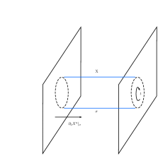
Figure 1: $X$ represents a periodic motion of an open string attached on two D-$3$ branes. The distance of the D-$3$ branes is the string length. The solid line denotes the string and dashed line represents the propagation.

For $\tilde{X}$, we get

$$②:\qquad\eta^{\mu\nu}\partial_{0}\tilde{X}_{\nu}|_{\tau} = 0,$$

$$\tilde{X}_{a}|_{\tau} = \tilde{Y}_{a},$$

$$\tilde{X}\left(\sigma,\tau\right) = \tilde{X}\left(\sigma+2\pi,\tau\right).$$ (2.29)

The relevant picture is a closed string propagating from one D-$3$ brane to another, as shown in Fig. 2. Since the time of propagation should be the same as $X$, the separation between the two D-branes is $t$. The equivalence of Fig. 1 and Fig. 2 was observed long time ago since they have the same topology. However, it is now clear that this open/closed duality is a consequence of the $O(D,D)$ symmetry.

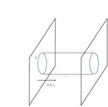
Figure 2: Closed string $\tilde{X}$ propagates from one D-$3$ brane to another one. The distance of the D-$3$ branes is time $t$. The solid line denotes the string and dashed line represents the propagation.

Next, we address the opposite limit, $r\ll c$. The metric becomes

$$\delta X^{a}\left(\frac{c^{2}}{r^{2}}\delta_{ab}\partial_{1}X^{b}\right)+\delta\tilde{X}_{\mu}\left(\frac{c^{2}}{r^{2}}\eta^{\mu\nu}\partial_{1}\tilde{X}_{\nu}\right)|_{\sigma} = 0,$$ (2.30)

$$\frac{c^{2}}{r^{2}}\delta_{ab}\delta X^{a}\partial_{0}X^{b}+\frac{c^{2}}{r^{2}}\eta^{\mu\nu}\delta\tilde{X}_{\mu}\partial_{0}\tilde{X}_{\nu}|_{\tau} = 0.$$ (2.31)

Since we want to keep the dimensionality of the D-branes unchanged, under this limit, $X$ is a closed string and $\tilde{X}$ is an open string. Following the same logic, the boundary conditions as $r\ll c$ are summarized as follows, for $X$,

$$③:\qquad\eta_{\mu\nu}\partial_{0}X^{\nu}|_{\tau} = 0,$$

$$X^{a}|_{\tau} = Y^{a},$$

$$X\left(\sigma,\tau\right) = X\left(\sigma+2\pi,\tau\right),$$ (2.32)

and for $\tilde{X}$,

$$④:\qquad\eta^{\mu\nu}\partial_{1}\tilde{X}_{\nu}|_{\sigma} = 0,$$

$$\tilde{X}_{a}|_{\sigma} = \tilde{Y}_{a},$$

$$\tilde{X}\left(\sigma,\tau\right) = \tilde{X}\left(\sigma,\tau+2\pi\frac{1}{t}\right).$$ (2.33)

Since the limit $r\ll c$ is equivalent to the limit $1/r\gg 1/c$, the distances of the $D$-branes under the two limits are approximate reciprocals. Thus, in the configuration $④$, the time of propagation is $T\backsimeq 1/t$, compared with $t$ in the configuration $①$. The corresponding pictures of these four configurations are depicted in Fig. 3.

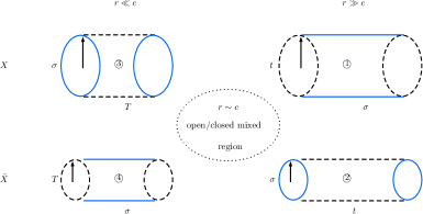
Figure 3: The four configurations in different limits. The solid lines denote the strings and dashed lines represent the propagations.

It should noted that we identify open or closed strings by the boundary conditions. One is able to do this near the asymptotic AdS region only. In the $r\sim c$ region, due to the EOM constraint (2.15), it is impossible to distinguish open or closed strings. They are entangled and the states are mixed states of open and closed strings. From traditional perspective, the physical picture may look puzzling.

A final remark of this subsection is that, one may notice in eqn. (2.16), on the $|_{\tau}$ boundary, we applied the first order EOM (2.15), which is valid only if the right hand side of EOM (2.4) vanishes,

$$\partial_{1}X^{A}\partial_{M}\mathcal{H}_{AN}\partial_{1}X^{N}=0.$$ (2.34)

For flat metric, this is true. However, for generically curved metrics, the story becomes very complicated. Of course, for non-compact topologies, it causes no trouble to our derivations. For the compact topology, remarkably, for the AdS geometry, since the metric is diagonal and only depends on the radial coordinate, it is not hard to see that only the radial direction $X^{a}$($\tilde{X}_{a}$) is affected. One can easily check that without using the first order EOM (2.15), the impacted boundary condition $\delta X^{a}\partial_{1}\tilde{X}_{a}+\delta\tilde{X}_{a}\partial_{1}X^{a}|_{\tau}=0$ perfectly fits our identifications of closed strings or open strings under different limits. This observation provides a specific technical reason for the requirement of AdS geometry.

2.2 Relations of the four configurations

From the derivations above, we see that the four configurations are $O(D,D)$ equivalent. To figure out the relations between them, it would be instructive to put the Kalb-Ramond field into the game.

After absorbing $f_{i}(\tau)$, the EOM is

$$g_{ij}\partial_{1}X^{j}-g_{ik}B^{kj}\partial_{1}\tilde{X}_{j}-\partial_{0}\tilde{X}_{i} = 0,$$

$$B^{ik}g_{kj}\partial_{1}X^{j}+\left(g^{ij}-B^{ik}g_{kl}B^{lj}\right)\partial_{1}\tilde{X}_{j}-\partial_{0}X^{i} = 0.$$ (2.35)

with boundary conditions

$$\delta X^{i}\left(g_{ij}\partial_{1}X^{j}-g_{ik}B^{kj}\partial_{1}\tilde{X}_{j}-\partial_{0}\tilde{X}_{i}\right)+\delta\tilde{X}_{i}\left(B^{ik}g_{kj}\partial_{1}X^{j}+\left(g^{ij}-B^{ik}g_{kl}B^{lj}\right)\partial_{1}\tilde{X}_{j}-\partial_{0}X^{i}\right)|_{\sigma} = 0,$$

$$\delta X^{i}\partial_{1}\tilde{X}_{i}+\delta\tilde{X}_{i}\partial_{1}X^{i}|_{\tau} = 0.$$

It is the right place to introduce the open/closed relation,

$$g_{ij} = \left(\hat{g}-\hat{B}\hat{g}^{-1}\hat{B}\right)_{ij},$$

$$B^{ij} = -\left(\frac{1}{\hat{g}+\hat{B}}\hat{B}\frac{1}{\hat{g}-\hat{B}}\right)^{ij},$$ (2.37)

derived from an $O(d,d)$ identification $\eta\mathcal{\hat{H}}\eta=\mathcal{H}$ as

$$\left(\begin{array}[]{cc}\hat{g}-\hat{B}\hat{g}^{-1}\hat{B}&\hat{B}\hat{g}^{-1}\\ -\hat{g}^{-1}\hat{B}&\hat{g}^{-1}\end{array}\right)=\left(\begin{array}[]{cc}g&-gB^{-1}\\ B^{-1}g&g^{-1}-B^{-1}gB^{-1}\end{array}\right).$$ (2.38)

With these identifications, the EOM is casted into

$$\partial_{1}X^{i} = B^{ij}\partial_{1}\tilde{X}_{j}+g^{ij}\partial_{0}\tilde{X}_{j},$$

$$\partial_{1}\tilde{X}_{i} = \hat{B}_{ij}\partial_{1}X^{j}+\hat{g}_{ij}\partial_{0}X^{j}.$$ (2.39)

The boundary conditions become

$$\delta X^{i}\left(g_{ij}\partial_{1}X^{j}+\hat{B}_{ik}\hat{g}^{kj}\partial_{1}\tilde{X}_{j}-\partial_{0}\tilde{X}_{i}\right)+\delta\tilde{X}_{i}\left(\hat{g}^{ij}\partial_{1}\tilde{X}_{j}+B^{ik}g_{kj}\partial_{1}X^{j}-\partial_{0}X^{i}\right)|_{\sigma} = 0,$$

$$\delta X^{i}\left(\hat{B}_{ij}\partial_{1}X^{j}+\hat{g}_{ij}\partial_{0}X^{j}\right)+\delta\tilde{X}_{i}\left(B^{ij}\partial_{1}\tilde{X}_{j}+g^{ij}\partial_{0}\tilde{X}_{j}\right)|_{\tau} = 0,$$ (2.40)

where we used the identity $\hat{B}\hat{g}^{-1}=-gB^{-1}$. It is obvious that the system is invariant under

$$X\leftrightarrow\tilde{X},\quad g\leftrightarrow\hat{g},\quad B\leftrightarrow\hat{B}.$$ (2.41)

Following the same logic as the case $B=0$, the decoupling of $X$ and $\tilde{X}$ only occurs in AdS background near the boundaries. Therefore, we get

$$\delta X^{a}\left(g_{ab}\partial_{1}X^{b}+\hat{B}_{ab}\hat{g}^{bc}\partial_{1}\tilde{X}_{c}-\partial_{0}\tilde{X}_{a}\right)+\delta\tilde{X}_{a}\left(\hat{g}^{ab}\partial_{1}\tilde{X}_{b}+B^{ab}g_{bc}\partial_{1}X^{c}-\partial_{0}X^{a}\right)$$

$$+\delta X^{\mu}\left(g_{\mu\nu}\partial_{1}X^{\nu}+\hat{B}_{\mu\rho}\hat{g}^{\rho\nu}\partial_{1}\tilde{X}_{\nu}-\partial_{0}\tilde{X}_{\mu}\right)+\delta\tilde{X}_{\mu}\left(\hat{g}^{\mu\nu}\partial_{1}\tilde{X}_{\nu}+B^{\mu\rho}g_{\rho\nu}\partial_{1}X^{\nu}-\partial_{0}X^{\mu}\right)|_{\sigma} = 0,$$

$$\delta X^{a}\left(\hat{B}_{ab}\partial_{1}X^{b}+\hat{g}_{ab}\partial_{0}X^{b}\right)+\delta\tilde{X}_{a}\left(B^{ab}\partial_{1}\tilde{X}_{b}+g^{ab}\partial_{0}\tilde{X}_{b}\right)$$

$$\delta X^{\mu}\left(\hat{B}_{\mu\nu}\partial_{1}X^{\nu}+\hat{g}_{\mu\nu}\partial_{0}X^{\nu}\right)+\delta\tilde{X}_{\mu}\left(B^{\mu\nu}\partial_{1}\tilde{X}_{\nu}+g^{\mu\nu}\partial_{0}\tilde{X}_{\nu}\right)|_{\tau} = 0.$$ (2.42)

Moreover, to have the decoupling in asymptotic regions, we suppose

$$B^{-1}g=-\hat{g}^{-1}\hat{B}\sim 1.$$ (2.43)

It is clear that $g,B,\hat{g}$ and $\hat{B}$ have the same monotonicity. Under the limit $g_{\mu\nu}\gg 1$ and $g_{ab}\ll 1$, the boundary conditions are

$$\delta X^{\mu}\left(g_{\mu\nu}\partial_{1}X^{\nu}\right)+\delta\tilde{X}_{a}\left(\hat{g}^{ab}\partial_{1}\tilde{X}_{b}\right)|_{\sigma} = 0,$$

$$\delta X^{\mu}\left(\hat{B}_{\mu\nu}\partial_{1}X^{\nu}+\hat{g}_{\mu\nu}\partial_{0}X^{\nu}\right)+\delta\tilde{X}_{a}\left(B^{ab}\partial_{1}\tilde{X}_{b}+g^{ab}\partial_{0}\tilde{X}_{b}\right)|_{\tau} = 0.$$ (2.44)

The consistent choices of the boundary conditions are

$$g_{\mu\nu}\partial_{1}X^{\nu}|_{\sigma} = 0,$$

$$X^{a}|_{\sigma} = Y^{a},$$

$$X\left(\sigma,\tau\right) = X\left(\sigma,\tau+2\pi t\right),$$

$$\mathrm{open\;string\;metric}: g.$$ (2.45)

and

$$\hat{g}^{\mu\nu}\partial_{0}\tilde{X}_{\nu}|_{\tau} = 0,$$

$$\tilde{X}_{a}|_{\tau} = \tilde{Y}_{a},$$

$$\tilde{X}\left(\sigma,\tau\right) = \tilde{X}\left(\sigma+2\pi,\tau\right),$$

$$\mathrm{closed\;string\;metric}: \hat{g}.$$ (2.46)

The boundary condition of $X$ in eqn. (2.45) precisely represents a commutative open string since $B$ does not show up and it is not a combination of Neumann and Dirichlet boundary conditions. It is well known that, to have a non-commutative theory, $B$ must be present in the boundary conditions. The metric is nothing but the open string metric $g$. On the other hand, by the similar reason, the boundary condition (2.46) of $\tilde{X}$ describes a commutative closed string. However, it is very instructive to notice that the metric of $\tilde{X}$ is precisely the closed string metric $\hat{g}$. Though $B$ or $\hat{B}$ are not explicitly exhibited in the boundary conditions, they have the same magnitudes of $g$ and $\hat{g}$. Therefore, the transformation between $g$ and $\hat{g}$ is still the non-trivial open/closed relation (2.37). Thus we have the answer for the second question proposed in the introduction:

The open/closed relation does connect commutative open string and commutative closed string theories.

On the other hand, if we choose $g_{\mu\nu}\ll 1$ and $g_{ab}\gg 1$, $X$ becomes commutative closed string with metric $g$ and $\tilde{X}$ becomes commutative open string with metric $\hat{g}$.

Bearing in mind we have three configurations: open-open, closed-closed and open-closed. In the open-open configurations, as we show in [17, 19], even with a non-vanishing $B$, there exist both non-commutative and commutative theories for the dual fields. The same story exists in closed-closed configuration. Therefore, we have the open-closed, commutative/non-commutative relations as in Fig. 4.

Figure 4: Commutative open and closed strings are connected in the asymptotic AdS region by $O(D,D)$. Either open strings or closed strings rotate back and forth between commutative and non-commutative theories by $O(D,D)$ transformations.

It is now easy to figure out the relations between the four states in the open-closed configuration, as summarized in Fig. 5.

It worth noting that we only addressed the compact topology of the worldsheet for open strings. We know that the $O(D)$ in $O(D,D)$ is actually non-compact $D(1,D-1)$ group, therefore, when rotating closed strings to compact open string worldsheet, the elements should be in the compact subgroup of $O(D,D)$. On the other hand, as we mentioned before, non-compact open string worldsheet also works perfectly, then the rotations ought to be the non-compact subgroups of $O(D,D)$. It would be of importance to explicitly construct the specific subsets for various manifolds in future works.

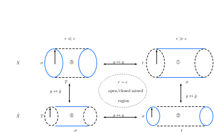
Figure 5: The $O(D,D)$ transformations between the four states in the open-closed configuration. The solid lines denote the strings and dashed lines represent the propagations.

3 The low energy effective implications and AdS/CFT

In the corresponding low energy limits, the relations among the four configurations in Fig. 5 have important consequences. For convenience, we list the properties of these configurations in Table 2. We know that the couplings of low energy effective theories are determined by the separation of $D$-branes. When the separation is large, the propagation of closed strings becomes far away. The massive modes have no contribution and we only need to consider the massless sector. But the open string length is big, the massive modes have significant contributions and therefore the gauge coupling is large. Oppositely, when the $D$-brane distance is small, supergravity approximation breaks down, while the massless sector of open strings dominates. Therefore, the low energy effective partners of the four configurations are listed in Table 3 and depicted in Fig. 6. As we explained in the last section, the compactness of the open string worldsheets do not affect the equivalence, our discussions on the low energy effective theories are general.

In the low energy effective theories, as shown in [17, 19], the relation ($①\leftrightarrow④$) is related to the Seiberg-Witten map between the commutative and non-commutative gauge theories. In string cosmology, the scale-factor duality ($B=0$) and its extension ($B\not=0$) are realizations of the transformation between ($②\leftrightarrow③$) as addressed in [20], and references therein. Moreover, considering the strength of the couplings, it should represents the S-duality. The descendant of ($②\leftrightarrow④$) in the low energy limit is conjectured as the weak gauge/weak gravity duality in literature. To our best knowledge, there is no conjectured relation for ($①\leftrightarrow③$) in the low energy effective theories, probably because both of them are strongly coupled and less interesting.

The most interesting duality is the low energy version of ($①\leftrightarrow②$) . From our previous arguments, the $AdS_{5}$ background is a necessity to decouple $X$ and $\tilde{X}$, which leads to the open-closed configuration. The decoupling only happens near the boundaries. Their low energy partners are precisely the weak gravity and strong gauge theory. All these properties are in agreement with AdS/CFT correspondence! This observation provides a practical way to prove AdS/CFT correspondence by getting the relevant low energy effective theories. Moreover, our results predict the intermediate mixed region. In this region, the string is neither open nor closed. The dual fields are coupled by the EOM (2.15). It is conceivable that, in the low energy limit, the gravity and gauge theory are entangled in the intermediate region as indicated by some recent conjectures. In the AdS/CFT correspondence, the gauge field concerned is $SU(N)$ Yang-Mills theory. It turns out that non-abelian and abelian gauge theories are also related by $O(D,D)$ symmetries [19].

Another duality of the strong gravity and weak gauge theory, deduced from ($③\leftrightarrow④$) represents the higher spin theory [7], attracted tremendous attention in recent years. Due to the success of AdS/CFT, it is natural to discuss the dual strongly coupled gravitational theory at short distance $r/\sqrt{\alpha^{\prime}}\ll 1$. Under this limit, the massive string states become massless since $m^{2}\sim r^{2}/\alpha^{\prime}$, and string theory reduces to the higher spin gravity. After the reduction, the modified gauge symmetry involves higher spin fields. Moreover, it is remarkable that the well-established higher spin theory in AdS₃/CFT₂ has a group $SO\left(2,2\right)$ [21], which is also consistent with our results.

From the off-diagonal configurations, we also observed the existence of strong/weak gauge duality and strong/weak gravity duality. The former one ($①\leftrightarrow④$) is consistent with the electromagnetic duality in abelian theories and its non-abelian extension [22, 23]. Once all the five dualities exist, one can of course anticipate a duality between the weak and strong gravity, as indicated by ($②\leftrightarrow③$).

	$r\ll c$	$r\gg c$
$X$	$③$ closed string (in near-horizon geometry)	$①$ open string (on the boundary)
$\tilde{X}$	$④$ open string (on the boundary)	$②$ closed string (in near-horizon geometry)

Table 2: The properties of the four configurations

	Short $r$	Long $r$
Open string	$④$ weak gauge theory	$①$ strong gauge theory
Closed string	$③$ strong gravitational interaction	$②$ weak gravitational interaction

Table 3: The corresponding low energy effective theories

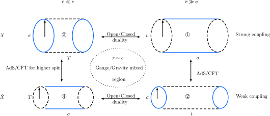
Figure 6: Predicted duality web in the low energy limits.

4 Summary and discussion

In summary, we generalized the Tseytlin’s action to an $O(D,D)$ invariant nonlinear double sigma model. We investigated the boundary conditions carefully and found, besides the usual open-open and closed-closed configurations for the dual fields, there does exist the open-closed configuration. It is remarkable that all the open and closed configurations are equivalent under $O(D,D)$ symmetries. This observation proves the equivalence of the open and closed string descriptions in string theory. To have the open-closed configuration, it is crucial to decouple the dual fields near the boundary. Surprisingly, it turns out that the decoupling can only happen in AdS geometry. From the symmetry group of M theory, we can identify that the AdS spacetime is precisely $AdS_{5}$. We then explicitly showed that the open/closed relation really connects commutative open strings and commutative closed strings, as its name indicates. We thus proved that the open/closed relation and open/closed duality are all $O(D,D)$ symmetries. Moreover, when consider the low energy limits, our results have predictions for AdS/CFT, higher spin theory, and a weak/weak as well as a strong/strong dualities between gauge theory and gravity. The Seiberg duality and another weak/strong gravitation duality are also present. The web of the dualities is a realization of $O(D,D)$ symmetry in the low energy effective theories.

There are several remarks we want to address. Though for the open-open and closed-closed configurations, the Tseytlin’s action can reduce to the Polyakov action after removing $X$ or $\tilde{X}$ with the corresponding EOM and boundary conditions, for the open-closed configuration addressed in this paper, effectively, there is no boundary conditions since they can be transformed to the identical form as the EOM. Therefore, one can not remove half of the degrees of freedom and the Tseytlin’s action has more physical implications than the Polyakov action.

The $r\sim c$ region, where the string is in mixed states of open and closed, is of great importance and interest. It is prompt to study it carefully and one can expect some non-trivial information can be extracted.

Constructing the low energy effective theories of the Tseytlin’s action is of course very important. It is not very hard to get the low energy limits of the open-open and closed-closed configurations. But the low energy limits of the open-closed configurations are not straightforward. Moreover, when considering the quantum theory, the gauge fixing is also subtle. However, once the low energy effective theories are obtained, we believe all the current dualities can be understood much better. Especially, since the Gauge/Gravity duality deals with weakly coupled theories on both sides, one can expect we may get some instructions to verify the duality.

Our calculation predicts the various dualities only in the background of AdS. The dS/CFT correspondence proposed in [24] is not compatible with our derivations. However, from the symmetry group of M theory, it is more precise to restrict our predictions to five dimensional spacetime. We thus can not exclude the dS/CFT correspondence from other dimensionality.

It would be of interest to incorporate SUSY into the theory. One may get more information about the required geometry, say, like $AdS_{5}\times S^{5}$? It will provide more evidence for the theory.

In this paper, we chose $X$ to be open or closed in different limits to keep the dimensionalities of the D-brane pair. However, at least in pure math, it is perfectly good to choose $X$ to be always open and $\tilde{X}$ to be always closed in both limits, or vice versa. This choice makes the two D-branes have mutual co-dimensionalities. Does this indicate that there exist some symmetries between different dimensional D-branes? A related question is that as we know, in the open-open configuration, the dimensionality of the D-brane is determined by the Neumann boundary condition of $X$ or the Dirichlet boundary conditions of $\tilde{X}$, then which choice is closer to the reality?

The closed string field theory (CSFT) is well-known for its complexity. The action is non-polynomial, which makes the CSFT is intractable. On the other hand, the open string field theory (OSFT) is much easier to deal with, though still very complicated, and has great progresses in the last twenty years. Our results, the equivalence of the open/closed string in the asymptotical AdS, provide a possible direction to attack the CSFT problems by transferring them to the corresponding OSFT problems.

Since we do not know how to define M theory yet, it is a promising way to generalize the Polyakov theory to $E_{D}$ covariant theories. It is reasonable to expect some non-perturbative features may be captured in these extensions. Furthermore, they may be also of help to the construction of M theory itself.

Acknowledgements We are especially indebted to B. Feng for innumerous illuminating discussions and his warm encouragement. We would like to acknowledge helpful discussions with our collegues Y. He, T. Li, Bo Ning, D. Polyakov and Z. Sun. This work is supported in part by the NSFC (Grant No. 11175039 and 11375121 ) and the Fundamental Research Funds for the Central Universities.

References

- [1] A. Sen, “Twisted black p-brane solutions in string theory,” Phys. Lett. B 274, 34 (1992) [hep-th/9108011]. S. F. Hassan and A. Sen, “Twisting classical solutions in heterotic string theory,” Nucl. Phys. B 375, 103 (1992) [hep-th/9109038]. J. Maharana and J. H. Schwarz, “Noncompact symmetries in string theory,” Nucl. Phys. B 390, 3 (1993) [hep-th/9207016]. C. M. Hull and P. K. Townsend, “Unity of superstring dualities,” Nucl. Phys. B 438, 109 (1995) [hep-th/9410167].
- [2] A. Sen, “Strong - weak coupling duality in four-dimensional string theory,” Int. J. Mod. Phys. A 9, 3707 (1994) [hep-th/9402002].
- [3] N. Seiberg and E. Witten, “String theory and noncommutative geometry,” JHEP 9909, 032 (1999) [hep-th/9908142].
- [4] G. T. Horowitz and J. Polchinski, “Gauge/gravity duality,” In *Oriti, D. (ed.): Approaches to quantum gravity* 169-186 [gr-qc/0602037].
- [5] P. Di Vecchia, A. Liccardo, R. Marotta and F. Pezzella, “Gauge / gravity correspondence from open / closed string duality,” JHEP 0306, 007 (2003) [hep-th/0305061].
- [6] G. T. Horowitz and A. Strominger, “Black strings and P-branes,” Nucl. Phys. B 360, 197 (1991). J. M. Maldacena, “The Large N limit of superconformal field theories and supergravity,” Adv. Theor. Math. Phys. 2, 231 (1998) [hep-th/9711200]. E. Witten, “Anti-de Sitter space and holography,” Adv. Theor. Math. Phys. 2, 253 (1998) [hep-th/9802150].
- [7] M. A. Vasiliev, “Higher spin gauge theories in four-dimensions, three-dimensions, and two-dimensions,” Int. J. Mod. Phys. D 5, 763 (1996) [hep-th/9611024]. I. R. Klebanov and A. M. Polyakov, “AdS dual of the critical O(N) vector model,” Phys. Lett. B 550, 213 (2002) [hep-th/0210114].
- [8] E. Malek, “U-duality in three and four dimensions,” arXiv:1205.6403 [hep-th].
- [9] A. A. Tseytlin, “Duality Symmetric Formulation Of String World Sheet Dynamics,” Phys. Lett. B 242, 163 (1990). A. A. Tseytlin, “Duality symmetric closed string theory and interacting chiral scalars,” Nucl. Phys. B 350, 395 (1991).
- [10] J. Maharana and J. H. Schwarz, “Noncompact symmetries in string theory,” Nucl. Phys. B 390, 3 (1993) [hep-th/9207016].
- [11] J. H. Schwarz and A. Sen, “Duality symmetric actions,” Nucl. Phys. B 411, 35 (1994) [hep-th/9304154].
- [12] D. Andriot, M. Larfors, D. Lust and P. Patalong, “A ten-dimensional action for non-geometric fluxes,” JHEP 1109, 134 (2011) [arXiv:1106.4015 [hep-th]]. D. Andriot, M. Larfors, D. Lust and P. Patalong, “(Non-)commutative closed string on T-dual toroidal backgrounds,” JHEP 1306, 021 (2013) [arXiv:1211.6437 [hep-th]]. C. D. A. Blair, “Non-commutativity and non-associativity of the doubled string in non-geometric backgrounds,” arXiv:1405.2283 [hep-th]. A. Betz, R. Blumenhagen, D. Lï¿œst and F. Rennecke, “A Note on the CFT Origin of the Strong Constraint of DFT,” JHEP 1405, 044 (2014) [arXiv:1402.1686 [hep-th]].
- [13] W. Siegel, “Two vierbein formalism for string inspired axionic gravity,” Phys. Rev. D 47, 5453 (1993) [hep-th/9302036]. W. Siegel, “Superspace duality in low-energy superstrings,” Phys. Rev. D 48, 2826 (1993) [hep-th/9305073]. W. Siegel, “Manifest duality in low-energy superstrings,” In *Berkeley 1993, Proceedings, Strings ’93* 353-363, and State U. New York Stony Brook - ITP-SB-93-050 (93,rec.Sep.) 11 p. (315661) [hep-th/9308133].
- [14] C. Hull and B. Zwiebach, “Double Field Theory,” JHEP 0909, 099 (2009) [arXiv:0904.4664 [hep-th]]. C. Hull and B. Zwiebach, “The Gauge algebra of double field theory and Courant brackets,” JHEP 0909, 090 (2009) [arXiv:0908.1792 [hep-th]]. O. Hohm, C. Hull and B. Zwiebach, “Background independent action for double field theory,” JHEP 1007, 016 (2010) [arXiv:1003.5027 [hep-th]]. O. Hohm, C. Hull and B. Zwiebach, “Generalized metric formulation of double field theory,” JHEP 1008, 008 (2010) [arXiv:1006.4823 [hep-th]].
- [15] M. J. Duff, “Duality Rotations In String Theory,” Nucl. Phys. B 335, 610 (1990). M. J. Duff and J. X. Lu, “Duality Rotations In Membrane Theory,” Nucl. Phys. B 347, 394 (1990).
- [16] D. S. Berman, N. B. Copland and D. C. Thompson, “Background Field Equations for the Duality Symmetric String,” Nucl. Phys. B 791, 175 (2008) [arXiv:0708.2267 [hep-th]]. D. S. Berman and D. C. Thompson, “Duality Symmetric Strings, Dilatons and O(d,d) Effective Actions,” Phys. Lett. B 662, 279 (2008) [arXiv:0712.1121 [hep-th]]. N. B. Copland, “Connecting T-duality invariant theories,” Nucl. Phys. B 854, 575 (2012) [arXiv:1106.1888 [hep-th]]. N. B. Copland, “A Double Sigma Model for Double Field Theory,” JHEP 1204, 044 (2012) [arXiv:1111.1828 [hep-th]]. D. S. Berman and D. C. Thompson, “Duality Symmetric String and M-Theory,” arXiv:1306.2643 [hep-th]. K. Lee and J. H. Park, “Covariant action for a string in "doubled yet gauged" spacetime,” Nucl. Phys. B 880, 134 (2014) [arXiv:1307.8377 [hep-th]].
- [17] D. Polyakov, P. Wang, H. Wu and H. Yang, “Non-commutativity from the double sigma model,” JHEP 1503, 011 (2015) [arXiv:1501.01550 [hep-th]].
- [18] D. Lust, “T-duality and closed string non-commutative (doubled) geometry,” JHEP 1012, 084 (2010) [arXiv:1010.1361 [hep-th]].
- [19] P. Wang, H. Wu and H. Yang, “Unification of gauge theories through symmetries,” to appear.
- [20] H. Wu and H. Yang, “Double Field Theory Inspired Cosmology,” JCAP 1407, 024 (2014) [arXiv:1307.0159 [hep-th]]. H. Wu and H. Yang, “New Cosmological Signatures from Double Field Theory,” arXiv:1312.5580 [hep-th].
- [21] J. Engquist and O. Hohm, “Geometry and dynamics of higher-spin frame fields,” JHEP 0804, 101 (2008) [arXiv:0708.1391 [hep-th]].
- [22] C. Montonen and D. I. Olive, “Magnetic Monopoles as Gauge Particles?,” Phys. Lett. B 72, 117 (1977).
- [23] N. Seiberg, “Electric - magnetic duality in supersymmetric nonAbelian gauge theories,” Nucl. Phys. B 435, 129 (1995) [hep-th/9411149].
- [24] A. Strominger, “The dS / CFT correspondence,” JHEP 0110, 034 (2001) [hep-th/0106113].